Salford Systems Data Mining Conference, NY/Madrid, 2005

Kasindra MaharajRobert Ceurvorst

Applied Prediction Problems in Financial Services: A Comparison of TreeNet®, Random Forests® and CART®

http://www.http://www. synovatesynovate .com.com

About the Presenters…

1

Kasindra MaharajKasindra Maharaj is a Senior Statistician and Leader of Synovate’s Data Mining Practice. She is the foremost authority in the company on data mining, having completed over 20 courses and seminars in data mining techniques and applications, as well as in programming and advanced statistics. Kasindra has extensive expertise in complex segmentations that involve linking data from multiple sources, much to the benefit of clients in many industries for whom she has done them. It is in connection with such applications that she gained much of her experience with CART, TreeNet and Random Forests. Kasindra holds a B.Sc. in Mathematics/Statistics and a M.Sc. in Statistics from The University of the West Indies, Trinidad.

Contact Info: Contact Info: kasindra.maharaj@synovate.comkasindra.maharaj@synovate.com or (312) 526 or (312) 526 –– 42114211

Dr. Robert CeurvorstDr. Robert Ceurvorst is the head of Synovate’s Decision Systems group in the Americas, our global team of methodological and statistical experts. In his 24 years as a statistician with the company, Bob has worked with clients in virtually every industry and developed many of the statistical techniques and software that Synovate uses for segmentation, brand equity, pricing and quantifying the influence of predictors on a criterion. Bob obtained his Ph.D. in Quantitative Methods from Arizona State University.

Contact Info: Contact Info: robert.ceurvorst@synovate.comrobert.ceurvorst@synovate.com or (312) 526 or (312) 526 -- 40704070

Overview

2

At Synovate, we’ve used CART for many years and are strong advocates for this tool because of the minds that went into creating it.

Hence, when we were looking to expand our data mining capabilities in 2004 we looked at Friedman’s and Breiman’screations: TreeNet (TN) and Random Forests (RF), respectively. We were interested in adding one or both of them to our data mining toolbox.

Overview

3

Companies are driven to demonstrate ROI for any new or existing product, service or marketing activity.

Need stronger linkages between consumers’ behavior and their needs, attitudes and demographics

Leverage relationships to more efficiently and profitably target– product and service offerings and – marketing activity

TreeNet (TN) and Random Forests (RF) offer the potential to establish stronger linkages than one could achieve using other models.

Overview

4

Purpose of our research:

To compare CART, RF and TN for classification problems in both large and

small data sets, CART and TN together with response surface regression, for a

regression problem, in a large data set

We’re using a small sample because RF is supposed to work better on smaller samples and a large sample because TN should ‘win’ on moderate to large samples.

Our focus in this presentation is on using CART, RF and TN as pure prediction tools. Hence, our presentation does not explore the useful graphics RF and TN produce that assist the user in understanding the models at hand.

Two Case Studies

5

1. Small: Use demographic and behavioral information on 350 customers of a top-5 global insurance company to predict their assessment of their financial situation (a classification problem):

struggling becoming comfortable/just beginning to save and pay off

debt very comfortable/building assets or well-off financially

2. Large: Use credit card usage behaviors on over 25,000 customers of a large bank to predict:

whether or not the credit score is at least 720 (a classification problem)

the actual credit score (a regression problem)

6

Case Study – Insurance Data

Insurance Case Study

7

Data Source: A survey was conducted in 2004 for a global

insurance company that included 353 customers in a certain North American market of interest.

For this purpose, the 353 customers were randomly split into: o Learn sample: n = 253 and o Test sample: n = 100

From the survey, 36 predictors (behaviors & demographics) were selected to predict a household’s present financial situation tobetter target certain products and/or services to appropriate HHs:

1. Struggling 2. Becoming comfortable/just beginning to save and pay off debt3. Very comfortable and/or building assets

A good financial advisor can do this. But it is more efficient to use an algorithm/machine when we have 1000’s of customers.

Insurance Case Study – Listing of Predictors

8

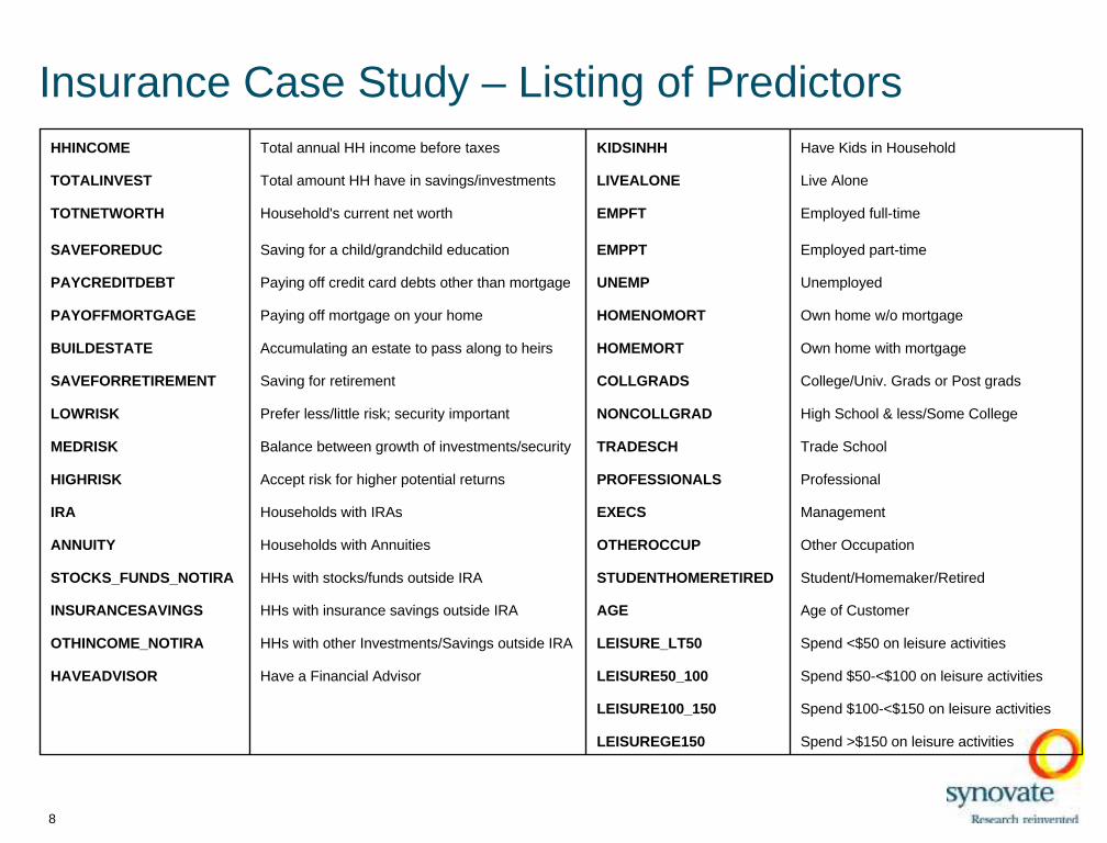
HHINCOME Total annual HH income before taxes KIDSINHH Have Kids in Household

TOTALINVEST Total amount HH have in savings/investments LIVEALONE Live Alone

TOTNETWORTH Household's current net worth EMPFT Employed full-time

SAVEFOREDUC Saving for a child/grandchild education EMPPT Employed part-time

PAYCREDITDEBT Paying off credit card debts other than mortgage UNEMP Unemployed

PAYOFFMORTGAGE Paying off mortgage on your home HOMENOMORT Own home w/o mortgage

BUILDESTATE Accumulating an estate to pass along to heirs HOMEMORT Own home with mortgage

SAVEFORRETIREMENT Saving for retirement COLLGRADS College/Univ. Grads or Post grads

LOWRISK Prefer less/little risk; security important NONCOLLGRAD High School & less/Some College

MEDRISK Balance between growth of investments/security TRADESCH Trade School

HIGHRISK Accept risk for higher potential returns PROFESSIONALS Professional

IRA Households with IRAs EXECS Management

ANNUITY Households with Annuities OTHEROCCUP Other Occupation

STOCKS_FUNDS_NOTIRA HHs with stocks/funds outside IRA STUDENTHOMERETIRED Student/Homemaker/Retired

INSURANCESAVINGS HHs with insurance savings outside IRA AGE Age of Customer

OTHINCOME_NOTIRA HHs with other Investments/Savings outside IRA LEISURE_LT50 Spend <$50 on leisure activities

HAVEADVISOR Have a Financial Advisor LEISURE50_100 Spend $50-<$100 on leisure activities

LEISURE100_150 Spend $100-<$150 on leisure activities

LEISUREGE150 Spend >$150 on leisure activities

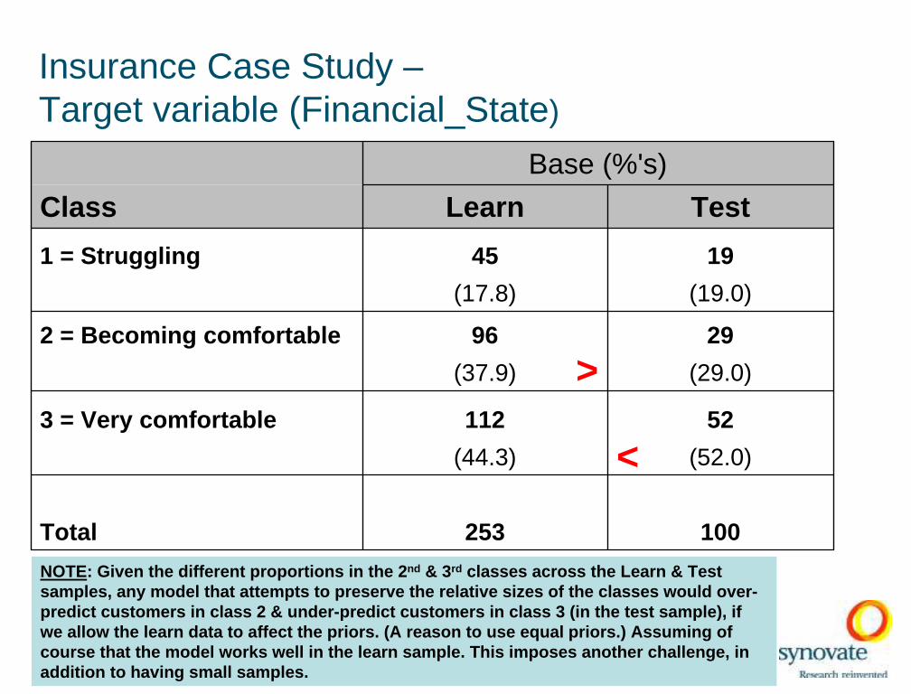
Insurance Case Study –Target variable (Financial_State)

9

Base (%'s)

Class Learn Test

1 = Struggling 45 19

(17.8) (19.0)

2 = Becoming comfortable 96 29

(37.9) (29.0)

3 = Very comfortable 112 52

(44.3) (52.0)

Total 253 100

>

<

NOTE: Given the different proportions in the 2 nd & 3rd classes across the Learn & Test samples, any model that attempts to preserve the relative si zes of the classes would over-predict customers in class 2 & under-predict customers in class 3 (in the test sample), if we allow the learn data to affect the priors. (A reason to use equal priors.) Assuming of course that the model works we ll in the learn sample. This imposes another challenge, in addition to having small samples.

10

Insurance Case Study: Predicting Households’ Financial State Using CART

Method: GiniPriors: Equal (for comparability)Minimum Cases in Parent Node: 15Minimum Cases in Terminal Node: 5 All other options: Defaults also

No. of Terminal Nodes in Optimal Tree: 11Overall Misclassification Rate: 46.0%

Insurance Case Study: Predicting Households’ Financial State Using CART

11

Test sample Predicted Class

Actual ClassTotal Cases

% Correct

1(N=23)

2 (N=33)

3(N=44)

1 = Struggling 19 47.37 9 10 0

(39.1) (30.3) (0.0)

2 = Becoming 29 41.38 6 12 11

Comfortable (26.1) (36.4) (25.0)

3 = Very 52 63.46 8 11 33

Comfortable (34.8) (33.3) (75.0)NOTES: (1) The %’s along the diagonal (in red) are what we call the purity rates. For example, of the twenty three customers predicted to be in cl ass 1, nine (39.1%) are actually in class 1. (2) We mainly focus on the diagonal elements & the predi cted bases in th e classes when assessing the usefulness of the model. (3) Because we used equa l priors, the predicted bases are more equal than the actual bases. (4) Total % Correctly Clas sified = Total Purity Rates.

With an overall classi fication of 54%, this model does approx. 60% better than chance. May obtain a better model with a larger sample.

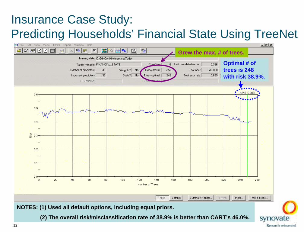
Insurance Case Study: Predicting Households’ Financial State Using TreeNet

12

NOTES: (1) Used all default op tions, including equal priors.

(2) The overall risk/misclass ification rate of 38.9% is better than CART’s 46.0%.

Grew the max. # of trees.

Optimal # of trees is 248 with risk 38.9%.

Insurance Case Study: Predicting Households’ Financial State Using TreeNet

Test Sample Predicted Class

Actual ClassTotal Cases

% Correct

1(N=28)

2(N=32)

3(N=40)

1 = Struggling 19 63.16 12 7 0

(42.9) (21.9) (0.0)

2 = Becoming 29 55.17 6 16 7

Comfortable (21.4) (50.0) (17.5)

3 = Very 52 63.46 10 9 33

Comfortable (35.7) (28.1) (82.5)

13

NOTES: (1) The purity & classification rates are better here than for CART.

(2) The predicted bases are more similar in size than for CART.

(3) We’re over-predictin g customers into class 1 and under -predicting customers in class 3.

(4) Total % Correctly Classi fied = 61%.

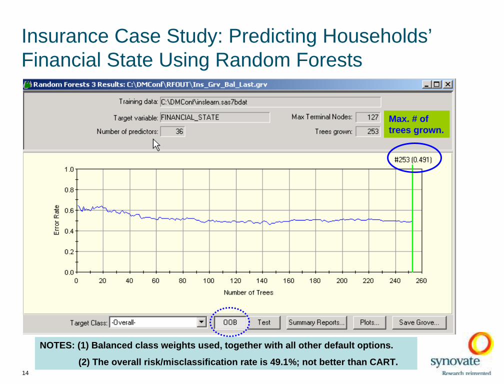
Insurance Case Study: Predicting Households’ Financial State Using Random Forests

14

NOTES: (1) Balanced class weights used, together with all ot her default options.

(2) The overall risk/misclassification r ate is 49.1%; not better than CART.

Max. # of trees grown.

Insurance Case Study: Predicting Households’ Financial State Using Random Forests

15

NOTES: (1) Balanced class weights used, together with all ot her default options.

(2) The overall risk/misclassification r ate is 41.0%; almost as good as TN.

Max. # of trees grown.

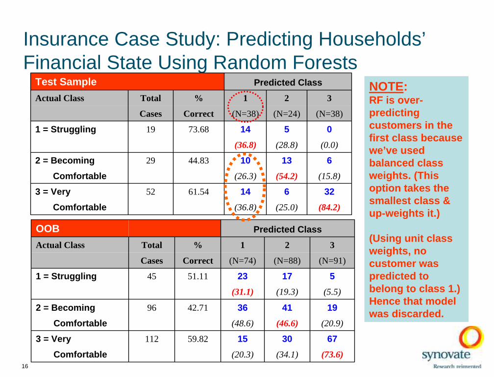
Insurance Case Study: Predicting Households’ Financial State Using Random Forests

16

OOB Predicted Class

Actual Class Total % 1 2 3

Cases Correct (N=74) (N=88) (N=91)

1 = Struggling 45 51.11 23 17 5

(31.1) (19.3) (5.5)

2 = Becoming 96 42.71 36 41 19

Comfortable (48.6) (46.6) (20.9)

3 = Very 112 59.82 15 30 67

Comfortable (20.3) (34.1) (73.6)

(84.2)(25.0)(36.8)Comfortable

3261461.54523 = Very

(15.8)(54.2)(26.3)Comfortable

6131044.83292 = Becoming

(0.0)(28.8)(36.8)

051473.68191 = Struggling

(N=38)(N=24)(N=38)CorrectCases

321% Total Actual Class

Predicted ClassTest Sample NOTE: RF is over-predicting customers in the first class because we’ve used balanced class weights. (This option takes the smallest class & up-weights it.)

(Using unit class weights, no customer was predicted to belong to class 1.) Hence that model was discarded.

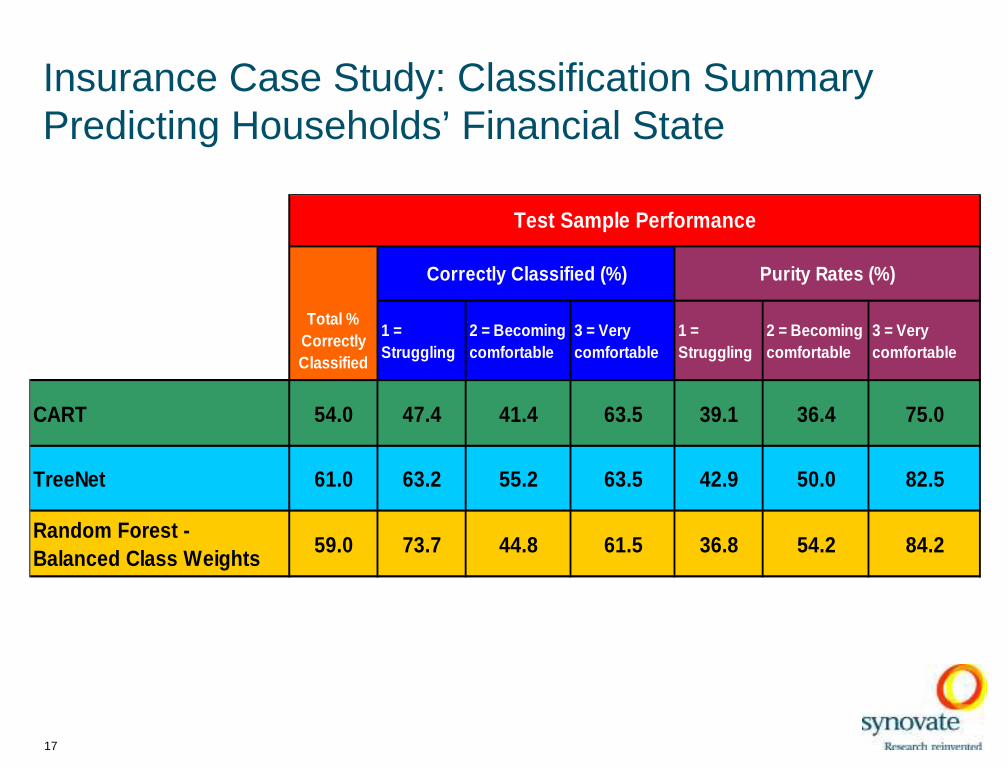
Insurance Case Study: Classification SummaryPredicting Households’ Financial State

Total % Correctly Classified

1 = Struggling

2 = Becoming comfortable

3 = Very comfortable

1 = Struggling

2 = Becoming comfortable

3 = Very comfortable

CART 54.0 47.4 41.4 63.5 39.1 36.4 75.0

TreeNet 61.0 63.2 55.2 63.5 42.9 50.0 82.5

Random Forest - Balanced Class Weights

59.0 73.7 44.8 61.5 36.8 54.2 84.2

Correctly Classified (%) Purity Rates (%)

Test Sample Performance

17

18

Insurance Case Study: Predicting Households’ Financial State

Conclusions:

Ü TreeNet actually produced the best results if we take into account both the purity rates and the predicted class sizes --even with such a small sample, wh ere we expected RF to ‘win’.

Ü RF has the most difficult time ma tching the original distribution of the learn and test samples using balanced or unit class weights.

ÜWith such a small data set, we find the time taken to run CART, RF & TN comparable. All techniques took 4 to 6 seconds (real time), even when TN was request ed to produce all possible plots.

Case Study – Bank Data

Classification

Bank Case Study

20

Data Source: Database information from a large bank with a

random sample of customers across North America.

For this purpose, the sample of 26,046 customers was split into two data sets:Ü Learn sample – 20,934 customersÜ Test sample – 5,112 customers

From the database, 8 predictors were selected to predict whether or not a customer had a good FICO score. (A customer has a good FICO score if his/her score is at least 720.)

These predictors reflect activity on the bank’s own credit card, not on other cards the customer uses that affect his or her credit score.

Bank Case Study – Variables Used

21

Target Variables(From credit agency):

FICO FICO Score (200-900) (For Regression)

HI_LOW High: FICO Score=>720 = 1, Low = -1 (For Classification)

Predictors:(Bank Source only)

ACCT_AGE Account age in months

NPURCH Avg. # Purchases/Mo. over past 6 mos (P6M)

NCASH Avg. # Cash Withdrawals/Mo. over P6M

AVGPURCH Avg. $ Purchases/Mo. over P6M

AVGCASH Avg. $ Cash Withdrawals/Mo. over P6M

AVGBAL Avg. Balance over P6M

LOWBAL Lowest Balance over P6M

BALTREND P6M Balance Trend

Bank Case Study – ClassificationTarget variable (Hi_Low)

22

Base (%'s)

Classes Learn Test

-1 = Low Scores 8701 2136

(credit score<720) (41.6) (41.8)

1 = High Scores 12233 2976

(credit score>=720) (58.4) (58.2)

Total 20934 5112

NOTE: The distributions in the learn & t est samples are close, in both classes, so we don’t expect to have the problem s encountered with the insurance data.

23

Bank Case Study – Classification Predicting High/Low Credit Scores Using CART

Method: GiniPriors: Equal (for comparability)Minimum Cases in Parent Node: 150Minimum Cases in Terminal Node: 50 All other options: Defaults, also

No. of Terminal Nodes in Optimal Tree: 60Overall Misclassification Rate: 26.4%

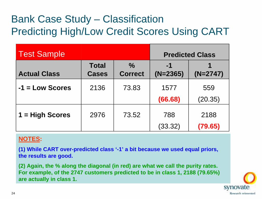
Bank Case Study – Classification Predicting High/Low Credit Scores Using CART

24

NOTES:

(1) While CART over-predicted class ‘-1’ a bit because we used equal priors, the results are good.

(2) Again, the % along the di agonal (in red) are what we call the purity rates. For example, of the 2747 customers predicte d to be in class 1, 2188 (79.65%) are actually in class 1.

Test Sample Predicted Class

Actual ClassTotal

Cases%

Correct-1

(N=2365)1

(N=2747)

-1 = Low Scores 2136 73.83 1577 559

(66.68) (20.35)

1 = High Scores 2976 73.52 788 2188

(33.32) (79.65)

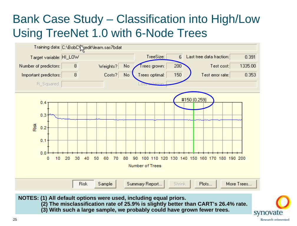
Bank Case Study – Classification into High/Low Using TreeNet 1.0 with 6-Node Trees

25

NOTES: (1) All default options were used, including equal prio rs. (2) The misclassification rate of 25.9% is slightly be tter than CART’s 26.4% rate.(3) With such a large sample, we pr obably could have grown fewer trees.

Bank Case Study – Classification into High/Low Using TreeNet 1.0 with 6-Node Trees

26

NOTES:

(1) TN over-predicted the low (-1) class a bit more than CART did ; using equal priors.

(2) Purity rates are both very close to those obtained in CART.

Test Sample Predicted Class

Actual ClassTotal

Cases%

Correct-1

(N=2421)1

(N=2691)

-1 = Low Scores 2136 75.42 1611 525

(66.54) (20.51)

1 = High Scores 2976 72.78 810 2166

(33.46) (80.49)

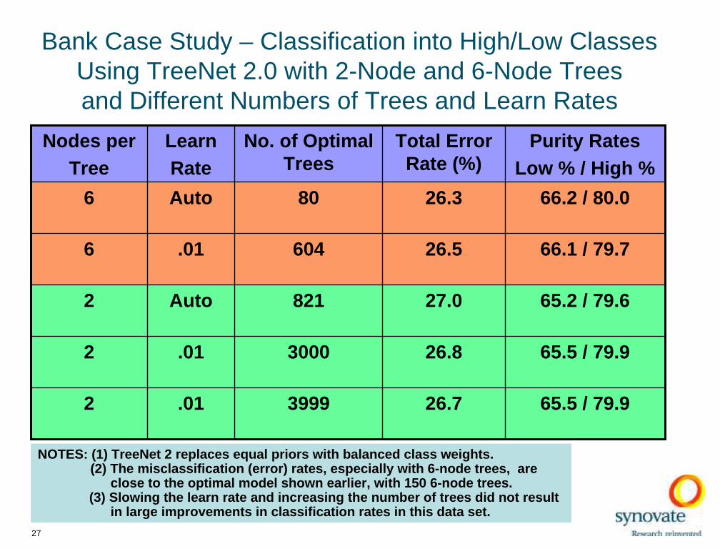
Bank Case Study – Classification into High/Low Classes Using TreeNet 2.0 with 2-Node and 6-Node Treesand Different Numbers of Trees and Learn Rates

27

Nodes perTree

LearnRate

No. of Optimal Trees

Total Error Rate (%)

Purity RatesLow % / High %

6 Auto 80 26.3 66.2 / 80.0

6 .01 604 26.5 66.1 / 79.7

2 Auto 821 27.0 65.2 / 79.6

2 .01 3000 26.8 65.5 / 79.9

2 .01 3999 26.7 65.5 / 79.9

NOTES: (1) TreeNet 2 replaces equal pr iors with balanced class weights. (2) The misclassifi cation (error) rates, especially with 6-node trees, are

close to the optimal model shown earlier, with 150 6-node trees.(3) Slowing the learn rate and increasing the number of trees did not result

in large improvements in classif ication rates in this data set.

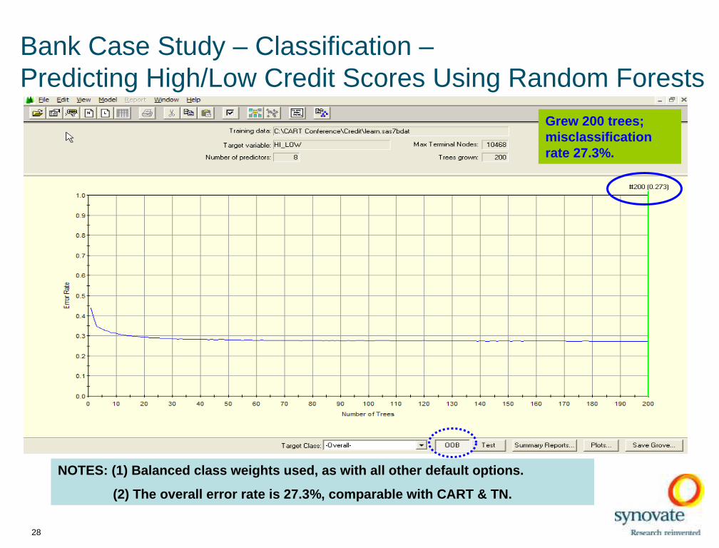
Bank Case Study – Classification –Predicting High/Low Credit Scores Using Random Forests

28

NOTES: (1) Balanced class weights used , as with all othe r default options.

(2) The overall error rate is 27.3 %, comparable with CART & TN.

Grew 200 trees; misclassification rate 27.3%.

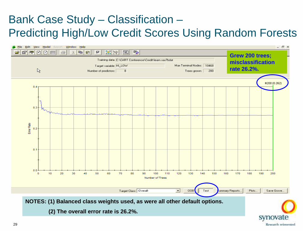
Bank Case Study – Classification –Predicting High/Low Credit Scores Using Random Forests

29

NOTES: (1) Balanced class weights used , as were all othe r default options.

(2) The overall error rate is 26.2%.

Grew 200 trees; misclassification rate 26.2%.

Bank Case Study – Classification –Predicting High/Low Credit Scores Using Random Forests

NOTES:

(1) As for TN, the results are comparable to CART.

(2) RF predicted test group sizes closer to actual than CART or TN.

(3) RF is time consuming with such a large data set.

Test SampleActua l Clas s Tota l % -1 1

Cas e s Co rre c t (N=23 4 8 ) (N=2 7 6 4 )

-1 = Low Scores 2 1 3 6 7 3 .6 0 1572 564(6 6 .9 5 ) (20 .41 )

1 = High Scores 2 9 7 6 7 3 .9 3 776 2200(33.05) (79 .60 )

Predicted Class

30

OOBActua l Clas s Tota l % -1 1

Cas e s Corre c t (N=9605) (N=11329)

-1 = Low Scores 8701 7 2 .46 6305 2396(65 .64 ) (21 .15 )

1 = High Scores 1 2 2 3 3 7 3 .02 3300 8933(34 .36 ) (78 .85 )

Predicted Class

Bank Case Study – Classification - Predicting High/Low Scores Using Logistic R. S. Regression

We used logistic response surface regression with the same 8 predictors.

Required a normalizing transformation to reduce the skewness and kurtosis of the predictors.

The model included

• 8 linear terms,

• 8 quadratic terms, and

• 28 interaction terms

31

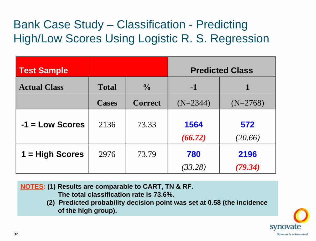
Bank Case Study – Classification - Predicting High/Low Scores Using Logistic R. S. Regression

32

Test Sample Predicted Class

Actual Class Total % -1 1

Cases Correct (N=2344) (N=2768)

-1 = Low Scores 2136 73.33 1564 572

(66.72) (20.66)

1 = High Scores 2976 73.79 780 2196

(33.28) (79.34)

NOTES: (1) Results are comparable to CART, TN & RF. The total classification rate is 73.6%.

(2) Predicted probability decision poi nt was set at 0.58 (the incidence of the high group).

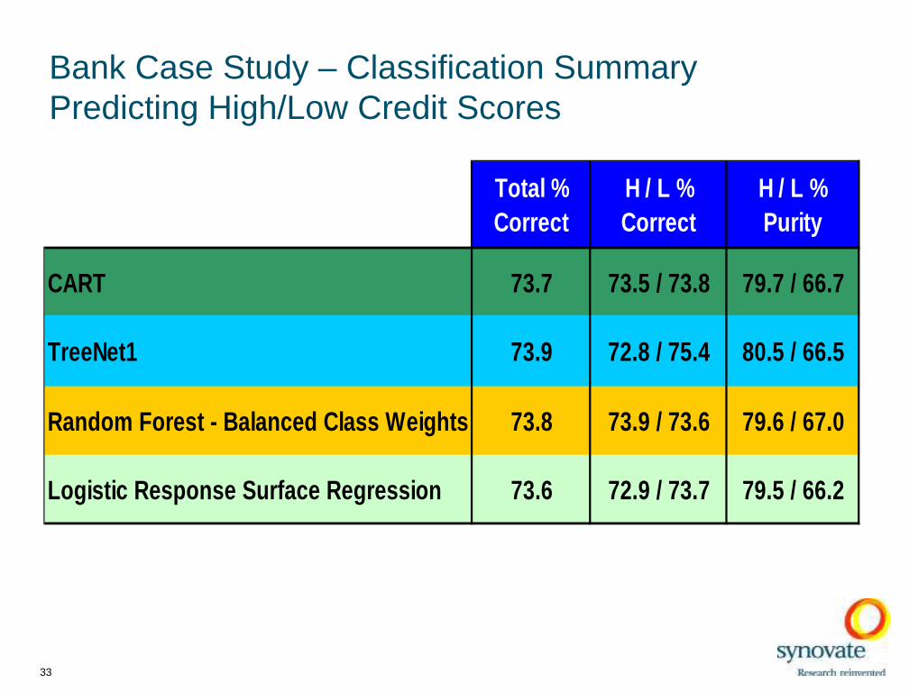
Bank Case Study – Classification Summary Predicting High/Low Credit Scores

Total %Correct

H / L %Correct

H / L %Purity

CART 73.7 73.5 / 73.8 79.7 / 66.7

TreeNet1 73.9 72.8 / 75.4 80.5 / 66.5

Random Forest - Balanced Class We ights 73.8 73.9 / 73.6 79.6 / 67.0

Logistic Response Surface Regressi on 73.6 72.9 / 73.7 79.5 / 66.2

33

Bank Case Study – Classification –Predicting High/Low Credit Scores

34

Conclusions:

Time is what differentiates all four techniques employedTime is what differentiates all four techniques employed. Even after . Even after building all plots, TN took just under a minute to run. However,building all plots, TN took just under a minute to run. However,RF took just over 6 minutes. RF took just over 6 minutes.

Logistic regression took more time and ‘care’ to program and runLogistic regression took more time and ‘care’ to program and run. . The predictors required normalization (which is not necessary foThe predictors required normalization (which is not necessary for r CART, TN or RF) and quadratic terms and interactions had to be CART, TN or RF) and quadratic terms and interactions had to be coded. coded.

Because of the nature of this data set (90% of the response surfBecause of the nature of this data set (90% of the response surface ace being explained by the 8 linear effects in the model), being explained by the 8 linear effects in the model), anyany of of these techniques should be able to do well, and did. these techniques should be able to do well, and did.

35

Case Study – Bank Data

Regression

Bank Case Study - Regression -Predicting Credit Scores

Here we use the same learn and test samples as were used for the classification problem.

Recall that the sample of 26,046 customers was randomly split into two data sets:

o Learn sample – 20,934 customerso Test sample – 5,112 customers

For our regression problem, we predict a customer’s FICO scoreusing the same 8 predictors used in the classification problem.

36

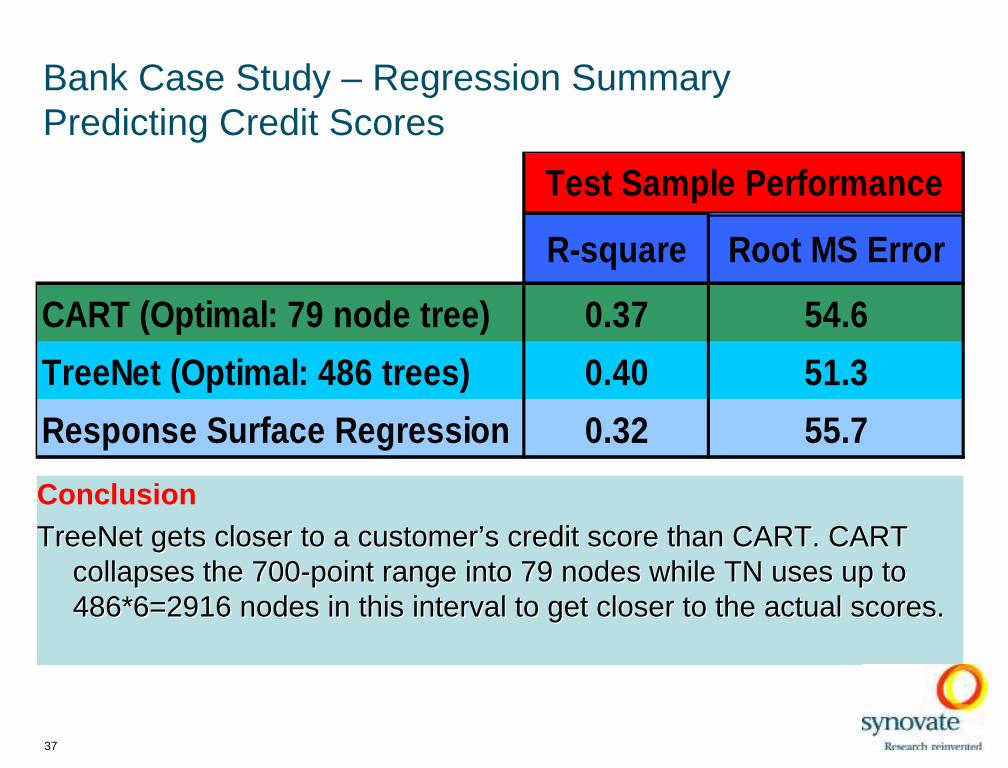
Bank Case Study – Regression Summary Predicting Credit Scores

R-square Root MS Error

CART (Optimal: 79 node tree) 0.37 54.6

TreeNet (Optimal: 486 trees) 0.40 51.3

Response Surface Regression 0.32 55.7

Test Sample Performance

ConclusionTreeNet gets closer to a customer’s credit score than CART. CARTTreeNet gets closer to a customer’s credit score than CART. CART

collapses the 700collapses the 700--point range into 79 nodes while TN uses up to point range into 79 nodes while TN uses up to 486*6=2916 nodes in this interval to get closer to the actual sc486*6=2916 nodes in this interval to get closer to the actual scores.ores.

37

Bank Case Study – Prediction of FICO ScoresUsing TreeNet 2.0* with 2-Node and 6-Node Treesand Different Numbers of Trees and Learn Rates

38

Nodes perTree

No. of Optimal Trees

Absolute Error R-Squared

6 486 41.8 .399

6* 508 41.9 .395

2* 821 43.1 .367

2* 1149 43.1 .368

NOTES: (1) Increasing the number of trees did not significantly affect prediction accuracy. (2) 6-node trees dete ct interactions; 2-node trees do no t. Therefore, the difference

between the performance of 2-node and 6-node trees is an indication of thepresence of interactions.

Final Conclusion on CART, TreeNet & Random Forests

39

For our purposes, TN works better.For our purposes, TN works better.

⊗⊗ TN takes much less time to run than RF & not much more than TN takes much less time to run than RF & not much more than CART for our large sample. CART for our large sample.

⊗⊗ TN was more accurate than CART or RF in our small sample.TN was more accurate than CART or RF in our small sample.

⊗⊗ TN worked well on both small and large classification problems. TN worked well on both small and large classification problems.

⊗⊗ TN gives us the added advantage of having a regression option thTN gives us the added advantage of having a regression option that at RF does not yet have. RF does not yet have.

⊗⊗ TN offers the HuberTN offers the Huber--M option (a plus) while CART has the least M option (a plus) while CART has the least absolute deviation.absolute deviation.

⊗⊗ RF models seem to work better on the test samples than the OOB RF models seem to work better on the test samples than the OOB sample in both data sets even though the insurance test sample wsample in both data sets even though the insurance test sample was as different then the learn sample.different then the learn sample.

While our presentation did not cover the graphics produced by thWhile our presentation did not cover the graphics produced by these tools, ese tools, TN produces simple, effective plots to help users understand theTN produces simple, effective plots to help users understand the effect effect of variables in the model. of variables in the model.

40

Thank you!