k-Multi-preference query over road networksmla.sdu.edu.cn/.../0/35/2E/BF6E60C9E709C3BDFF0007… ·...

ORIGINAL ARTICLE

k-Multi-preference query over road networks

Peiguang Lin1,2 • Yilong Yin1,2 • Peiyao Nie1

Received: 21 October 2015 /Accepted: 30 March 2016 / Published online: 19 April 2016

� Springer-Verlag London 2016

Abstract Nowadays, the road network has gained more

and more attention in the research area of databases.

Existing works mainly focus on standalone queries, such as

k-nearest neighbor queries over a single type of objects

(e.g., facility like restaurant or hotel). In this paper, we

propose a k-multi-preference (kMP) query over road net-

works, involving complex query predicates and multiple

facilities. In particular, given a query graph, a kMP query

retrieves of the top-k groups of vertices (of k facility types)

satisfying the label constraints and their aggregate dis-

tances are the smallest. A naıve solution to this problem is

to enumerate all combinations of vertices with k possible

facility types and then select the one with the minimum

sum distance. This method, however, incurs rather high

computation cost due to exponential possible combina-

tions. In addition, the existing solutions to other standalone

queries are for a single type of facilities and cannot be

directly used to answer kMP queries. Therefore, in this

paper, we propose an efficient approach to process a kMP

query, which utilizes an index with bounded space and

reduces the computation cost of the shortest path queries.

We also design effective pruning techniques to filter out

false alarms. Through our extensive experiments, we

demonstrate the efficiency and effectiveness of our pro-

posed solutions.

Keywords kMP query � Road network � Query graph �Approximation distance matrix � Shortest path

1 Introduction

Nowadays, it has become increasingly important for people

to manipulate and interact with spatial data in many real

applications such as the location-based services (LBS),

geographic information systems (GIS), navigation systems

(GPS), map services (Google Map or MapQuest), and

mobile computing systems. The ultimate goal of services in

these applications is to enable users to quickly retrieve their

interested spatial objects.

In the aforementioned applications, spatial data are usu-

ally constrained by road networks, and the actual distance

between any two objects is given by the length of the shortest

path between them. Previous works usually studied queries

that involve one type of facilities in road networks, for

example, report the nearest restaurant [i.e., nearest neighbor

(NN)] with respect to the user’s current location [1] or a

restaurant that has the smallest summed distance to a group

of users [i.e., aggregate nearest neighbor (ANN)] [2–4].

In practice, however, users may specify much more

complex query predicates involving multiple facilities,

which is much more challenging to solve than one single

query over one type of facility. What is worse, some

complex queries cannot even be answered efficiently by

using the existing solutions. For example, a traveler may

want to find a set of facilities including a hotel, a restau-

rant, and a museum, such that the summation of distances

among these three facilities is the smallest. The naıve

solution of answering this query is to enumerate all pos-

sible combinations of three facilities and then select the

one with the minimum summed distance among these

& Peiguang Lin

[email protected]

Peiyao Nie

[email protected]

1 School of Computer Science and Technology, Shandong

University of Finance and Economics, Jinan, China

2 School of Computer Science and Technology, Shandong

University, Jinan, China

123

Pers Ubiquit Comput (2016) 20:413–429

DOI 10.1007/s00779-016-0913-0

http://crossmark.crossref.org/dialog/?doi=10.1007/s00779-016-0913-0&domain=pdf

http://crossmark.crossref.org/dialog/?doi=10.1007/s00779-016-0913-0&domain=pdf

facilities. Clearly, this naıve solution is quite expensive in

terms of the computation cost and thus cannot be applied to

large scale of networks with huge number of facilities,

especially when the user needs a fast response.

In this paper, we study an important and useful query,

namely k-multi-preference (kMP) query in road networks,

which involves complex query predicates over multiple

facilities. Specifically, given a user-specified multi-prefer-

ence pattern (i.e., query graph) with constraints on attri-

butes of each facility, a kMP query retrieves k groups of

facilities from a road network, such that, in each group, the

vertices fulfill constraints of query graph (in terms of

facility types and attributes on each facility), and the

aggregate road network distances connecting these vertices

are the smallest. Based on the returned results, a user is

able to enforce a sense of sequence of target facilities to be

visited. The kMP query has many useful applications, and a

typical example is illustrated as follows.

Running example: Consider a traveler who wants to have

a tour around a new city. Assume that he/she has two

candidate plans, A and B, which are two possible kMP

queries, as shown in Fig. 1, where k = 4.

Plan A (3-day plan): As illustrated in Fig. 1a, the traveler

stays in a hotel (H), and he plans to visit three facilities

within 3 days, for example, a museum (M), a park (P), and

a shopping mall (S), each facility per day.

Plan B (1-day plan): As illustrated in Fig. 1b, the traveler

first checks in a hotel (H). Then, within 1 day, he will visit

a museum (M), followed by a park (P) and a shopping mall

(S), and finally come back to hotel (H).

Plan requirements: For Plan A, the traveler plans to stay

in a 5-star hotel (H), which has price within 1000–3000

HKD, the museum (M) must be an art museum, and the

shopping mall (S) should have an apple store. On the other

hand, in Plan B, the traveler may require a 5-star hotel

(H) with price 1000–3000 HKD, and a shopping mall

(S) selling a particular souvenir.

In Fig. 1, each edge is corresponding to a traveling path

for the traveler to drive from one endpoint (facility) to

another on the road network. The weight of the edge

implies the total traveling distance on this edge. Note that,

in our example, Plans A and B have query graphs of star

and ring shapes, respectively. Nevertheless, our proposed

solutions in this paper are generic to tackle the kMP

problem with the query graph of arbitrary shape (i.e.,

allowing arbitrary graph-based patterns).

Different from the traditional graph matching prob-

lem, in our kMP problem, the traveler may specify

preferences about the places that he/she wants to stay/

visit, which involve constraints on arbitrary attribute

data types. For example, he/she might only be interested

in 5-star hotels, history museums, parks having restau-

rants in it, and shopping malls selling a specific sou-

venir. In other words, he/she can specify any constraints

related to the facilities (as described in the running

example). In this case, the traveler can exactly issue a

kMP query to retrieve top-k groups of facilities (in-

cluding H, M, P, and S) that minimize his/her total

traveling distance in the road network.

Challenges In the running example above, there are

totally Hj j � Mj j � Pj j � Sj j combinations of facilities in

the worst case, where :j j is the number of facilities satis-

fying query predicates (e.g., 5-star hotel). Thus, a

straightforward way to tackle the kMP problem is to

repeatedly use these facility combinations as query

point(s) of nearest neighbor (NN) or aggregate nearest

neighbor (ANN) queries and then combine the results.

However, this method clearly incurs high computation cost

due to large number of facility combinations.

In brief, the query answering of a kMP query is chal-

lenging for two main reasons. First, predicates involving

facility types, and constraints on facilities are complex and

costly to check. Second, it is inefficient to compute the

shortest path distance between two vertices on the road

network. In addition, given a very large road network, it is

not possible to put its entire index in the memory. To

address the challenges above, we propose an efficient

approach to answer kMP queries, based on a shortest path

approximation scheme, which results in satisfactory prun-

ing power and query answering-time.

In particular, we highlight our contributions as follows:

1. We propose a novel query, k-multi-preference (kMP),

in the context of large road networks in Sect. 3.

2. We propose a general framework for handling kMP

queries over large road networks in Sect. 5. Specifi-

cally, a filter-and-refine strategy is applied in order to

shrink the searching space and reduce the computation

cost.

3. We propose effective and nontrivial filtering methods

in Sect. 5. In addition, we design a cost model to select

the shortest path tree with high pruning powers.

(a) (b)

1

1

1

2 2

S

H

M P

S

H

M P

2 1

Fig. 1 An example of the k-multi-preference query. a Plan A, b Plan

B

414 Pers Ubiquit Comput (2016) 20:413–429

123

4. In Sect. 6, extensive experiments have been conducted

to demonstrate the efficiency and effectiveness of our

proposed approaches to answer kMP queries on both

real and synthetic datasets.

In addition, Sect. 2 reviews related works on both road

network modeling, and query processing over road net-

works or large graphs. Section 7 concludes this paper.

2 Related work

Road network modeling: Road networks combine geo-

graphic and graph-theoretic information in one structure.

The majority of studies consider a road network as a

general graph, directed [5–10] or undirected [2, 11–13]. On

the other hand, a number of previous works model a road

network as a planar graph (e.g., [14]). However, such a

planarity cannot be guaranteed in modern road network

datasets. This is because there are some cases with ‘‘edge-

crossing,’’ caused by tunnels and bridges in reality. In [15],

the authors conducted a series of experiments demon-

strating that, for an n-vertex road network, there will typ-

ically be Hffiffiffi

npð Þ road segment crossings when all those

segments are projected on the surface of a sphere using

their GPS coordinates.

Query processing over road network: Query processing

on road networks has been extensively studied [1, 2, 6–10,

12, 13], since its unique spatial and topological features.

Essentially, the kMP query distinguishes itself from the

existing works since it considers the pattern with multiple

predefined labels. To the best of our knowledge, this is the

first work to address the kMP query over road networks,

where the network distance is adopted as the distance

metric. With kMP, users may specify much more complex

query predicates involving multiple facilities, which is

much more challenging to solve than one single query over

one type of facility. The most relevant query, namely

Pattern Match, has been investigated in several works [16–

19]. There are two typical types of pattern matching

queries that are studied recently. The first is defined in

terms of subgraph isomorphism, which finds all subgraphs

of G that are isomorphic to a given query graph Q [16]. The

second one, which is much more relevant to our work, is

defined as follows [17]: Given a data graph G, a query

graph Q (with n vertices), and a parameter e, n vertices in

G can form a match to Q, if: (1) these n vertices in G have

the same labels as the corresponding vertices in Q; and (2)

for any two adjacent vertices v and u in Q (i.e., there is an

edge between v and u in Q), the distance between two

corresponding vertices in G is no larger than e. This query

returns all the matches of Q in G. In [20], the authors treat

taxi ridesharing problem as finding k-nearest neighbors

problem although it does not cover all challenges in min-

imizing system wide travel time and travel distance.

3 Problem definition

In this section, we give the formal definition of k-multi-

preference (kMP) query over a road network.

3.1 Data model

Road network model: We naturally model a road network

as a vertex-labeled edge-weighted undirected graph. First,

we assume this graph is a nearly a planar graph. A typical

planar graph is a graph that can be drawn on a plane such

that there are no ‘‘edge crossings,’’ that is, edges intersect

only at their common vertices. In this paper, for simplicity,

we assume that there are only a small number of edge

crossings existing in the graph. This assumption is usually

not uncommon, especially when encountering the follow-

ing circumstances:

1. The dataset is extracted from a planar graph, e.g., from

satellite photos.

2. The application service can tolerate the inaccuracy that

is introduced by treating a nonplanar graph as a planar

graph.

3. The computing power is insufficient to handle the

index structure of query processing for nonplanar

graphs, or lead to unsatisfactory response time (e.g.,

cell phones or GPS devices).

Note that the only property related to our road network

model is Property 1, which will be discussed in Sect. 3.1.

Property 1 assumes that, for a given shortest path P and a

vertex v, the distances from v to all the vertices in P can

be approximated. This property is not uncommon in many

real road network datasets, having a very weak constraint

on the classical graph model. Thus, our data model is

general enough to capture the features of real road

networks.

Facilities and attributes: In addition to the graph

structure, each vertex in road networks is also associated

with a ‘‘facility type’’ and a number of ‘‘attributes.’’ A

‘‘facility’’ indicates the category of a vertex, such as

museum and hotel, whereas ‘‘attributes’’ are features pre-

defined for each facility type, for example, ‘‘star-level’’ and

‘‘price’’ can be considered as attributes of a ‘‘hotel.’’

Constraints on such facilities and attributes in vertices are

often specified by query graphs, which will be defined in

the next subsection.

Pers Ubiquit Comput (2016) 20:413–429 415

123

3.2 Definition of kMP queries

Query graph: A query graph GQ (VQ, EQ) is also an edge-

weighted graph, consisting of two pieces of information

below.

(A) The constraints on facilities types and attributes:

Each vertex is labeled with a facility type together

with a number of attributes.

(B) The route of visiting facilities: The weight of an edge

e(u, v) represents the number of times the user will

travel between u and v.

As mentioned above, in the query graph, some condi-

tions may be specified by users to constrain the ‘‘facility

type’’ and/or attributes of vertices. As in the previous

example of the trip plan, we list the domain of facility

types, and the domains/constraints of attribute values for

the facility ‘‘Hotel.’’ In real applications, such domains or

constraints can be specified by service providers or users.

Domain of facility types:

Hotel Museum Park Shopping mall

Domains/constraints of attributes for facility ‘‘Hotel’’:

Price (USD) Star-level Free-WIFI Swimming pool (USD/h)

500–1000 5-star Yes 10

1000–2000 4-star 20

2000–3000 3-star No 30

Above 3000 Others Free

The function of range constraints enables users to

specify each facility attribute with a subset of its domain of

attribute values. For a vertex v, we call this subset the range

constraints on an attribute A, denoted v.RC(A). Facilities

and attributes are associated with each vertex on both road

networks and query graphs. For instance, a user may be

only interested in hotels with attribute ‘Price’ being

‘500–1000’ or ‘2000–3000’, and then, on the query graph,

there is a vertex hq with ‘Hotel’ as facility type and attri-

bute constraint hq.RC(Price) = {‘500–1000’, ‘2000–

3000’}. Let h be a facility on the road network labeled with

‘Hotel’, if h.RC(Price) = {others, ‘2000–3000’}, and then,

h should be considered to be a vertex in the results; if

h.RC(Price) = {‘others’, ‘1000–2000’}, h should not be

considered.

kMP queries over a road network: We consider each

input kMP query as a weighted small graph GQ(VQ, EQ),

with each vertex associated with one type of facility and its

attributes, which determines the facility type and con-

straints on attributes. The edges and weights determine the

traveling plan among the facilities. Now, we formally

define the kMP query as follows.

Definition 1 (target vertex) Given a road network G(V,

E) and an input query graph GQ(VQ, EQ) where

VQ = {v1,…, vn}, the function wðvi; vjÞ denotes the weightof the edge ðvi; vjÞ.

A vertex ui in V is said to be a target vertex w.r.t. a

vertex vi in VQ, if and only if the following conditions hold:

1. vi and ui are of the same facility type;

2. for all attributes A belonging to this facility type,

|vi.RC(A) \ ui.RC(A)|[ 0.

Definition 2 (label match) Given a road network G(V, E)

and an input query graph GQ(VQ, EQ) where VQ = {v1,…,

vn}, the function wðvi; vjÞ denotes the weight of the edge

ðvi; vjÞ.

A set of n distinct vertices {u1,…, un} in V is said to be a

label match w.r.t. GQ, if and only if, for all i, ui is a target

vertex w.r.t. vi.

Definition 3 (label match distance) Given a road network

G(V, E) and an input query GQ(VQ, EQ) with edge-weight

function w(.), for a label match M w.r.t. GQ, the label

match distance (LMD) is defined as

LMDðMÞ ¼X

ðvi;vjÞ2EQ

wðvi; vjÞDistðui; ujÞ;

where Distðui; ujÞ denotes the shortest distance between uiand uj over G.

Definition 4 (k-multiple-preference query) Given a road

network G(V, E), an input query GQ(VQ, EQ) where

VQ = {v1,…, vn} and a user-defined parameter k, a k-

multiple-preference query is to find the top-k matches with

minimal LMDs.

4 Preliminary

4.1 Approximation oracle with connection set

An approximate distance oracle is a data structure which can

approximate the shortest path, via Distapðu; vÞ; for a (con-

nected) graph G = (V, E). If the reported Distapðu; vÞ; sat-isfies that Distðu; vÞ�Distapðu; vÞ� aDistðu; vÞ8u; v 2 V ,

the distance oracle is said to have multiplicative stretch a.Clearly, we expect the answer time and multiplicative

stretch to be as small as possible. One can see that the trade-

off is actually between the multiplicative stretch ð1þ eÞ andthe index space O ln =eð Þ, and e can be minimized by


123

utilizing all the memory space available. In this paper, we

limit the stretch no larger than 2 in order to guarantee sat-

isfactory pruning power, i.e., for a parameter e 2 ð0; 1�;Distðu; vÞ�Distapðu; vÞ� ð1þ eÞDistðu; vÞ:

Let P be the shortest path in a graph G. A pair (p, v) of

vertices where p is in P and v is in G is a connection for v

with respect to P. A set C of such connections covers v in G

with respect to P if, for every node p of P, there is a

connection (p, u) in C such that Distðp; vÞ�Distðu; vÞþDistðp; uÞ� ð1þ eÞDistðp; vÞ. Such a set is named con-

nection set w.r.t. P. In [21], it is proved that given a planar

graph G and a shortest path P, in linear time, one can

compute a set C of connections that covers all nodes of G

and that has at most 2 1e

� �

þ 1 connections per vertex v. In

real road network datasets, the number of connections

remains when there is no edge crossing existing on the

path. Note real road networks have only a very small

number of edge crossing a single path; therefore, the

number of connections can be estimated as O 1e

� �

, which

can be empirically confirmed in the experiments. The

sketch algorithm of finding those connections [22] is

illustrated as Algorithm 1.

_____________________________________________________

_____________________________________________________

Algorithm 1: Constructing_Connection_Set [4]Find the vertex a on P that is the nearest to vSet x=a, and iterate y through the vertexes from atowards the end-points of P. If (v,x) does not cover (v,y) within the approximation threshold, we add (v,y) and set x=y

Property 1 In a road network, for any shortest path P

and a given vertex v, Algorithm 1 can compute a connec-

tion set contains O 1e

� �

connections.

Intuitively, in order to minimize the index space, we

expect to find a minimal number of shortest paths such

that every vertex lays on at least one of them. Solely for

the shortest path (SP) query, we can consider this

problem as an optimization problem and find a near-

optimal set of paths (since it is NP-hard). In [22], a

graph decomposition technique based on LIPTON-TAR-

JAN separator is also proposed on SP queries, which

leads to slightly worse but also constant processing time.

However, another major factor dominating the computing

time of kMP is the huge number of combinations of

facilities. Therefore, we propose an index schema based

on one shortest path tree and associated pruning tech-

niques, which significantly reduce the number of

combinations.

4.2 Baseline method with LLR embedding

One straightforward way to process a kMP query is to

convert this problem into a variant of the pattern match-

ing query defined in [16]. We call this baseline method

‘‘D-join.’’ In the original setting of Gallagher [16], there

is constrictive edge-distance parameter d for ruling out

candidates. In particular, if ðvi; vjÞ 2 EQ and uiðujÞ is a

target vertex of viðvjÞ, then a label match containing

ui and uj can be considered as an output only if

Distðui; ujÞ� d.The essential difference between kMP and D-join is

twofold. First, each pattern matching query is associated

with an edge-length threshold, but kMP is not. Second,

kMP enables users to pose range constraints on vertex

labels, whereas the pattern matching does not support such

range constraints. Therefore, in order to perform the kMP

query answering efficiently, we generalize the method

proposed in [16] in the following way:

1. We propose a novel binary encoding method to

efficiently handle range constraints. With such a

method plugged in, a kMP query can be considered

as a pattern matching query, with the edge-distance

parameter equal to positive infinity;

2. During the processing of D-join, we ignore the weights

of edges on the query graph, so that the results are

candidate label matches; and

3. Lastly, we refine candidates by computing the

weighted sum of the edges, according to Definition

3, and obtaining their LMDs.

We dynamically maintain a top-k threshold for pruning

other candidates. In order to enable the pruning with such a

threshold, we apply an LLR embedding technique [21].

Specifically, LLR maps all vertices in G into points in a

vector space Rk, where k is the dimensionality of the vector

space. We briefly illustrate the embedding process as

follows:

1. Let Sn,m be a subset of randomly selected vertices in V.

Then, for any vertex v, we define Dðv; Sn;mÞ as the

distance from v to the closest vertex in Sn,m, that is,

Dðv; Sn;mÞ ¼ minu2Sn;mfDistðu; vÞg, where Dist(u, v) is

the shortest path distance from u to v on the road

network.

2. We randomly select H log2 Vj j� �

subsets to form the set

R ¼ fS1;1; . . .; S1;a; . . .; Sb;1; . . .; Sb;ag, where a ¼H log Vj jð Þ and b ¼ H log Vj jð Þ; hence, ba ¼ k.

3. The mapping function E: V ! Rk is defined as

follows: for any vertex v in V, we have

EðvÞ ¼ Dðv; S1;1Þ; . . .;Dðv; S1;aÞ; . . .;Dðv; Sb;1Þ; . . .;Dðv; Sb;aÞ;� �

;


123

4. Finally, in the converted vector space Rk, we use

DistRðu; vÞ to denote the distance between u and v, so

we have

DistRðu; vÞ ¼ maxn;m

jDðv; Sn;mÞ � Dðu; Sn;mÞ

Theorem 2.1 ([21]) Given two vertices u and v in G, dis-

tance, DistRðu; vÞ; between two corresponding points in the

converted vector spaceRk, and the shortest distanceDistðu; vÞbetween u and v in the original road network, we have:

DistRðu; vÞ�Distðu; vÞ

Lower bound of LMD: Therefore, by using the embed-

ding techniques above, we can estimate the lower bound,

LMDR; of LMD value for a label match, by using the

distance in the vector space.

In particular, by Definition 3, this lower bound is given

by:

LMDR ¼X

ðvi;vj2EQÞwðvi; vjÞDistRðui; ujÞ:

X

ðvi;vjÞ2EQ

wðvi; vjÞDistðui; ujÞ�X

ðvi;vjÞ2EQ

wðvi; vjÞDistRðui; ujÞ:

We obtain LMDR; as a lower bound of LMD (see proof

in [21]).

Therefore, we can apply LMDR; to reduce the costly

computation of (exact) LMDs. Finally, we refine the

remaining candidates by calculating their actual LMD

values. This way, the D-join baseline method can obtain k

patterns with minimal LMDs (i.e., kMP answers).

Although the D-join baseline method can correctly

retrieve kMP answers, there are two major flaws for road

networks of large sizes:

1. With the edge-distance parameter initially being positive

infinity at the beginning, the number ofmatching patterns

canbe toohuge tobehandled, since noneof themcould be

pruned by the edge-distance constraint. The pruning

bounds of D-join could be very loose, since the edge-

length threshold is first set to positive infinity. Consider a

kMP query with five vertexes in VQ, and there are 100

satisfactory facilities for each of them. Then, there will be

1010 matches as the result of joining tables!

2. To our best knowledge, there is no algorithm available

to support the exact shortest path query unless using

Oðn2Þ space is given for indexing, where n is the

number of vertices. A single match already requires

EQ

�

�

�

� shortest path queries. Since modern road networks

contain huge number of vertexes, such a response time

is not satisfactory for realistic applications.

5 Generic framework

In this subsection, we propose a generic framework for

answering k-multi-preference (kMP) queries over a road

network. Algorithm 2 depicts the pseudo-code of the kMP

framework. Specifically, algorithm kMP_Framework con-

sists of two portions, offline and online processing._____________________________________________________Algorithm 2 kMP_Framework {

// offline processing1: Constructing Approximation Distance Matrix2: Label each vertex by its distance to the root//online processing3: for each label match{4: if (branch-level pruning succeeds) 5: the whole branch is pruned and goto next branch6: else 7: perform match-level pruning8: update threshold best_so_far9: }

10: refine candidates and return kMP answers}_____________________________________________________

Offline processing: For the offline processing, in order to

efficiently obtain upper and lower bounds of pairwise

distance between vertices in road network, we create an

approximation oracle, namely approximation distance

matrix (line 1). This matrix can be used to enable our

online pruning method (i.e., match-level pruning discussed

in Sect. 5.2). Compared to the accurate distance Dist(u, v),

the error of approximated distance, Distapðu; vÞ, is boundedby an arbitrary small real number e, that is:

Distðu; vÞ�Distapðu; vÞ� ð1þ eÞDistðu; vÞ

To obtain a good matrix with high pruning power, we

propose to construct it by finding a shortest path tree T that

covers the entire road network and then decomposing T.

Then, the approximate answer (to a point-to-point shortest

path query) can be obtained within a constant time strictly

bounded by log2ð2e�1 þ 1Þ time cost, and overall Oðln =eÞindex space, where l is the number of leaf vertices in the

shortest path tree.

As a second step, the offline processing aims to label

each vertex with its distance to the root (line 2). This

precomputed data can be used by our branch-level pruning

method (discussed later in Sect. 5.2).

Online processing:

1. Filtering phase (lines 3–9): For each kMP query

GQ(VQ, EQ), we apply our proposed pruning methods,

namely branch-level pruning and match-level pruning,

to rule out false alarms of candidate matches. The

online process dynamically maintains a list of candi-

dates, and prune candidates alternatively by branch-

level pruning (line 4) and match-level pruning (line 7).


123

The rationale of the match-level pruning is to obtain

lower/upper bounds of LMD distances by utilizing the

guaranteed error of approximated distances. Since the

computation cost of exact LMD is high, instead, we com-

pute its lower/upper bounds at low costs via approximate

LMD (LMDap), which is obtained from the offline pre-

computed approximation distance matrix.

On the other hand, the branch-level pruning is essen-

tially based on the triangle inequality. This pruning tech-

nique is applied to avoid false alarms of target vertex

combinations.

2. Refinement phase (line 10): After the filtering phase,

we can obtain a number of candidates. We refine these

candidates, by calculating their exact distances in road

networks, and finally return actual kMP query answers

(line 10).

5.1 Offline processing with approximation oracle

To process a kMP query, encountering the fact that many

shortest distance queries may be generated, we consider

using the value range of approximate answers to prune,

which significantly shrinks the searching space.

Generally, for one match M, computing LMD(M) gen-

erally requires |EQ| shortest path queries, each of which

costs OðnÞ answer time (assuming no Oðn2Þ space avail-

able), i.e., O(|EQ|n) for computing LMD(M). One can see

that computing exact LMDs is very costly, especially when

there are many label matches. Since our concern is to find

the top-k matches, if we could find ranges of LMDs, which

are sufficient to rank the top-k matches, and the response

time is much faster than O(|EQ|n); consequently, the overall

processing time can be reduced significantly.

Lemma 1 (upper-bound pruning) Let best_so_far be the

upper bound of the LMD of the kth label matches the label

matches we have seen so far. A label match M can be safely

pruned, if it holds that LMD(M)[ best_so_far.

Running example:

Label match Lower bound Upper bound

M1 1 2

M2 1.5 2.5

M3 2.6 3

M4 (pruned) 3.1 3.2

Suppose k = 3, and we already have the above four ranges

of LMDs. Then, any label match M with LMD(M) whose

lower bound is larger than 3 is guaranteed not to be in the

answer set to be returned, so M4 can be safely pruned.

To enable the upper-bound pruning, we propose to use an

approximate distance to obtain the distance bounds. To be

clear, we do not accept approximate query answers, we only

apply the approximation as bounds to improve the compu-

tational efficiency. Through the above running example, we

see the bounds of LMD are very conductive for finding the

expected top-k answers, especially the bounds are very tight.

In following, we propose and describe an approximation-

based index, from which the bounds of a LMD can be

obtained very efficiently. For instance, suppose the

approximate value of LMD is obtained as c with multi-

plicative stretch a, and then, we have c as upper bound and

ðc=aÞ as lower bound. In addition, such index also facilitatespruning method to avoid enumerating unnecessary label

matches, illustrated in Sect. 6.2.

5.1.1 Constructing approximation distance matrix

We consider a shortest path tree T spanning the road net-

work. A shortest path tree is a subgraph of a given graph

constructed so that the distance between a selected root

node and all other nodes is minimal. Such a spanning tree

can be easily derived from the information obtained by

running a single instance of Dijkstra’s single-source

shortest path algorithm [23]. Suppose T is rooted at vertex

r, and then, the path from each leaf vertex v to r is their

shortest path in graph G. We call such a path branch path.

In other words, each pair (v, r) uniquely identifies a branch

path of T. Now we define an important concept—branch

segment.

Definition 5 (branch segment) Given a shortest path tree

T, a branch segment is an ordered sequence of vertices on a

branch path, in an ascending order of their distances to the

root.

There are two steps to build this approximation oracle—

first, we decompose the shortest path tree T into a set of

branch segments; second, we select a number of vertices on

each branch segment and build connection sets with

Algorithm 1 in order to construct the approximation dis-

tance matrix.

Branch-based decomposition: We find the branch path

containing the most vertices from T and remove the ver-

tices (with their incident edges) on the path from T. As a

result, T is decomposed into a set of subtrees {T1, T2,…}.

Then, we repeat the decomposition process recursively on

each of the subtrees, until the result is an empty set. One

can see that all the vertices are contained by exactly one

branch segment. During the recursion, branch segments

with no facility vertices are eliminated. It is clear that the

number of branch paths extracted from T is upper-bounded

by the number of leaf vertices of T.


123

_____________________________________________________Algorithm 3 Branch_based_Decomposition {

Input: a shortest path tree covering T all the vertices in G, an set Stree of sub-trees, an set Sbranch of branch segments(initially, Stree= Sbranch=∅)

Output: Sbranch1: Finding the branch path b with the maximal number of

labeled vertices 2: add b to Sbranch ;3: remove b from T, then T = T/b = { T1 , T2 , …Ts}4: for 1i ← to s5: add Ti to Stree6: for each sub-tree Tj in Stree7: if (Tj is a path)8: Stree = Stree – {Tj}, Sbranch = Sbranch {Tj};9: else Branch_based_Decomposition(Tj, Stree, Sbranch);}

_____________________________________________________

Remark A branch segment does not have to be a con-

nected graph. This feature is useful for the branch-level

pruning algorithm.

Approximation distance matrix: As a result of the

decomposition, T is split into a list of branch segments,

denoted as {S1,S2…Sl}. One can see that every vertex is

contained by exactly one branch segment, which is also a

shortest path over G. By applying the algorithm in

Sect. 6.3, we construct a n� l matrix as follows.

S1 S2 … Sl-1 Sl

V1 NULL C11 C1(l-1) C1l

V2 C21 NULL C2(l-1) C2l

…Vn-1 C(n-1)1 C(n-1)2 C(n-1)(l-1) NULL

Vn Cn1 Cn2 NULL Cnl

In the matrix, each cell (V, S) records either a NULL

value or a memory address pointing to a collection set of

v with respect to S. Note that the branch segments are also

shortest paths at this time. A NULL value occurs that v is on

the branch segment S. In particular, the root vertex contains

NULL value for each of its cells since it is on every branch

segment of T. We sort the branch segments by the number of

vertices they contains, i.e., S1 goes through the most number

of vertices, while Sl goes through the least.

On the other hand, a connection set C pointed by (V,

S) is constructed as a list below:

Note that the connections are ranked by the distance

they are from the root by ascending order, not from V. To

be clear, in the above data structures, the vertices Vi are

references of object instances of the vertices from the

shortest path tree T.

Now we explain why such index is particularly small. In

reality, the number of vertex representing the ‘intersec-

tions’ of roads is only the minority, while most vertices are

‘facilities’ over road segments. For instance, among the

vertices in ‘CA’ dataset (see Sect. 6), there are around 20k

for intersections and 80k for facilities. As illustrated in

Fig. 2, facilities are added on the graph, and the topological

structure would not be changed. Hence, the number of leaf

vertices of a shortest path tree also remains unchanged.

5.2 Pruning strategies

5.2.1 Match-level pruning

5.2.1.1 Query Distapðu; vÞ and approximate LMD The

rationale of match-level pruning is to use high-efficiency

approximate query answers as bounds of the exact answers.

This is because the exact answers are quite costly to obtain,

while the approximate answers are already sufficient to

filter out the majority of nonresult candidates for kMP

query.

We label each vertex u with its (only) branch segment,

and its distance from the root of T, denoted as u.s and u.d,

respectively. Then, for a pair (u, v), then two cells from the

approximation distance matrix could be located, i.e., (u,

v.s) and (v, u.s). We randomly take one, say (u, v.s), which

references to either a NULL value or a connection set C.

Obviously, NULL value indicates that u and v are in the

same branch segment, so we actually get the exact distance,

i.e., Distapðu; vÞ ¼ Distðu; vÞ ¼ u:d � v:dj j. More likely, we

compute the distance with connection set C according to

Fig. 2 Illustration of road modeling

Vertices on S Distance from V

V11 10

V21 15

V31 8

V41 16


123

the approximation distance matrix. Since C contains a list

of vertices ranked by their distances form the root, we

perform a binary search over the list and locate the two

vertices, denoted vi and vj that are the closest to v. Let diand dj be the associated distance in C, and then, we have

Distapðu; vÞ ¼ min di þ vi:d � v:dj jð Þ; dj þ vj:d � v:d�

�

�

�

� ��

.

Any point-to-point approximation distance can be

answered from the branch-based index schema with

O log e�1ð Þð Þ time cost. Thus, for any match M, an

approximate value of LMDðMÞ (denoted LMDapðMÞ) canbe calculated by querying each edge-distance in EQ. By

Definition 3, we have: LMDapðMÞ ¼P

ðvi;vjÞ2EQ

wðvi; vjÞDistap

ðui; ujÞ with O EQ

�

�

�

� log e�1ð Þ� �

time cost. We summarize the

pruning rule in the following theorem.

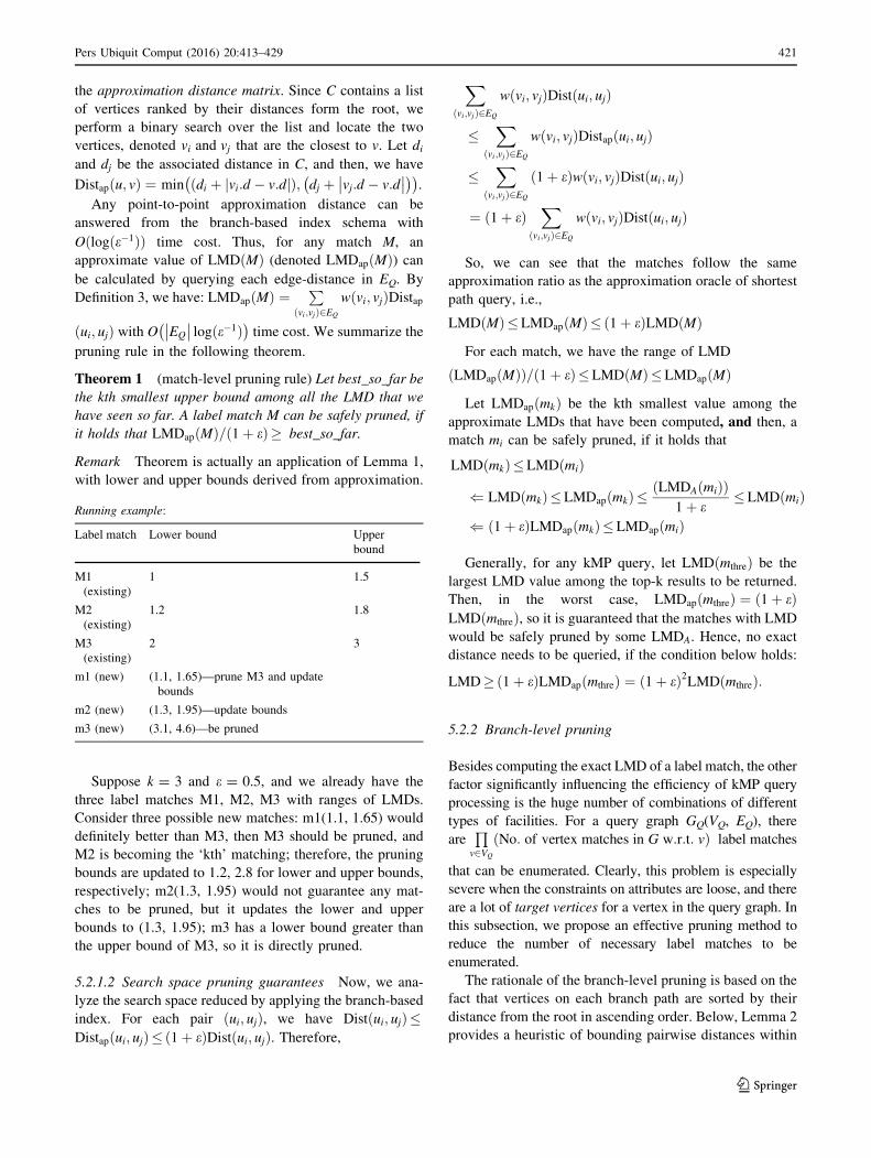
Theorem 1 (match-level pruning rule) Let best_so_far be

the kth smallest upper bound among all the LMD that we

have seen so far. A label match M can be safely pruned, if

it holds that LMDapðMÞ= 1þ eð Þ� best_so_far.

Remark Theorem is actually an application of Lemma 1,

with lower and upper bounds derived from approximation.

Running example:

Label match Lower bound Upper

bound

M1

(existing)

1 1.5

M2

(existing)

1.2 1.8

M3

(existing)

2 3

m1 (new) (1.1, 1.65)—prune M3 and update

bounds

m2 (new) (1.3, 1.95)—update bounds

m3 (new) (3.1, 4.6)—be pruned

Suppose k = 3 and e = 0.5, and we already have the

three label matches M1, M2, M3 with ranges of LMDs.

Consider three possible new matches: m1(1.1, 1.65) would

definitely better than M3, then M3 should be pruned, and

M2 is becoming the ‘kth’ matching; therefore, the pruning

bounds are updated to 1.2, 2.8 for lower and upper bounds,

respectively; m2(1.3, 1.95) would not guarantee any mat-

ches to be pruned, but it updates the lower and upper

bounds to (1.3, 1.95); m3 has a lower bound greater than

the upper bound of M3, so it is directly pruned.

5.2.1.2 Search space pruning guarantees Now, we ana-

lyze the search space reduced by applying the branch-based

index. For each pair ðui; ujÞ, we have Distðui; ujÞ�Distapðui; ujÞ� ð1þ eÞDistðui; ujÞ. Therefore,

X

ðvi;vjÞ2EQ

wðvi; vjÞDistðui; ujÞ

�X

ðvi;vjÞ2EQ

wðvi; vjÞDistapðui; ujÞ

�X

ðvi;vjÞ2EQ

ð1þ eÞwðvi; vjÞDistðui; ujÞ

¼ ð1þ eÞX

ðvi;vjÞ2EQ

wðvi; vjÞDistðui; ujÞ

So, we can see that the matches follow the same

approximation ratio as the approximation oracle of shortest

path query, i.e.,

LMDðMÞ�LMDapðMÞ� ð1þ eÞLMDðMÞ

For each match, we have the range of LMD

ðLMDapðMÞÞ=ð1þ eÞ�LMDðMÞ�LMDapðMÞ

Let LMDapðmkÞ be the kth smallest value among the

approximate LMDs that have been computed, and then, a

match mi can be safely pruned, if it holds that

LMDðmkÞ�LMDðmiÞ

( LMDðmkÞ�LMDapðmkÞ�ðLMDAðmiÞÞ

1þ e�LMDðmiÞ

( ð1þ eÞLMDapðmkÞ�LMDapðmiÞ

Generally, for any kMP query, let LMDðmthreÞ be the

largest LMD value among the top-k results to be returned.

Then, in the worst case, LMDapðmthreÞ ¼ ð1þ eÞLMDðmthreÞ, so it is guaranteed that the matches with LMD

would be safely pruned by some LMDA. Hence, no exact

distance needs to be queried, if the condition below holds:

LMD�ð1þ eÞLMDapðmthreÞ ¼ ð1þ eÞ2LMDðmthreÞ:

5.2.2 Branch-level pruning

Besides computing the exact LMD of a label match, the other

factor significantly influencing the efficiency of kMP query

processing is the huge number of combinations of different

types of facilities. For a query graph GQ(VQ, EQ), there

areQ

v2VQ

ðNo: of vertex matches in G w:r:t: vÞ label matches

that can be enumerated. Clearly, this problem is especially

severe when the constraints on attributes are loose, and there

are a lot of target vertices for a vertex in the query graph. In

this subsection, we propose an effective pruning method to

reduce the number of necessary label matches to be

enumerated.

The rationale of the branch-level pruning is based on the

fact that vertices on each branch path are sorted by their

distance from the root in ascending order. Below, Lemma 2

provides a heuristic of bounding pairwise distances within


123

two disjoint branch segments. This heuristic will lead to a

pruning rule to reduce the number of combinations. For any

two disjoint branch segments BS1 and BS2, we denote this

bound as PBbound(BS1, BS2).

Lemma 2 (pairwise branch bounding) Given two dis-

joint branch segments BS1 ¼ v1; v2; . . .; vxf g and BS2 ¼u1; u2; . . .; uyf g, BS1 \ BS1 ¼ ;; then for any distance

Distðvi; ujÞ where vi and uj belong to BS1 and BS2,

respectively, we have Distðvi; ujÞ� PB bound ðBS1;BS2Þ ¼ maxððv1:d � uy:dÞ; ðu1:d � vx:dÞÞ

Proof When ðv1:d � uy:dÞ� ðu1:d � vx:dÞ, By Defini-

tion 5, vertices in BS1 and BS2 are sequenced in ascending

order, so we have v1:d� vi:d8vi 2 BS1 ð1Þ

And uy:d� uj:d8uj 2 BS2 ð2ÞBy (1)–(2), v1:d � uy:d� vi:d � uj:d

Since for any pair of vertices, Distðvi; ujÞ�vi:d � uj:dj j � vi:d � uj:d; we have Distðvi; ujÞ� v1:d�uy:d

The case when ðv1:d � uy:dÞ\ðu1:d � vx:dÞ is sym-

metric. So the proof is completed.

Theorem 2 (branch-level pruning rule) Let best_so_far

be the upper bound of the LMD of the kth label matches

among the label matches we have seen so far. Given query

graph GQ(VQ, EQ), VQ = {v1, v2…, v|VQ|}, edge-weight

function w(.), and |VQ| disjoint branch segments {BS1,

BS2,…, BS|VQ|} such that for all i, BSi is a set of target

vertices w.r.t. vi.

For any label match m = {u1,…, u|VQ|} such that

8u 2 m; u 2S

VQ

q¼1

BSq, m can be safely pruned if holds that

X

ðvi;vjÞ2EQ

wðvi; vjÞPB bound ðBSi;BSjÞ� best so far

Running example: Now we consider query graph GQ(VQ,

EQ) where VQ = {vL, uL} EQ = {e = (vL, uL), w(e) = 1}.

As shown in Fig. 3, v is a target vertex of vL, while u1, u2,…ur, which are from the same branch segment, are target

vertices of uL. B1 and B2 are distances from the root to v and

u1, respectively. Since B2–B1[ best_so_for, the following

label matches can be pruned: {v, u1}, {v, u2}… {v, ur}.

5.3 Binary coding on range constraints

5.3.1 Binary encoding on road network

We assign each vertex a binary code representing its

facility information, which enables range constraints for

users. In this subsection, we propose a labeling-based index

method to enhance the searching capability over T corre-

sponding to the label constraints.

On the road network, we convert the information of

facility type and attributes into binary codes, with each bit

representing the ‘availability’ of one attribute value (‘1’ for

available and ‘0’ for unavailable, e.g., on attribute ‘price,’

the code of ‘500–1000’ being ‘1’ means there is a room

available priced from 500 to 1000 in this hotel). Then, each

vertex on the road network is associated with a binary

code, called the vertex’s Label. We denote the code of a

vertex v’s label value as LabelðvÞ. Specifically, for an

attribute with d domain values (e.g., for Star-level in the

example, d = 4), we assign d bits to each vertex on this

attribute. The reason for using d bits, rather than log2 d, is

that: First, one facility may fulfill multiple domain values

on one attribute, e.g., a hotel may have regular rooms

priced from ‘500–1000,’ and luxury suites priced ‘Above

3000’; second, such model enables users to have range

constraints on attributes, e.g., the star-level from ‘5-star to

3-star.’

Similarly, facility types and attributes of query graph

can be also converted into binary codes as same style as

road network. We adopt the same notation as well. How-

ever, each bit being ‘1’ on one attribute represents whether

the corresponding value is acceptable for the user. So on

attribute ‘price,’ the code of ‘500–1000’ and ‘Above 3000’

both being ‘1’ means any hotel is acceptable for the user if

there is a regular room priced from 500 to 1000 or a luxury

suite priced above 3000.

5.3.2 Determining vertex matches

Suppose there is a vertex v from the road network and a

vertex vq from the query graph, and v and vq have the same

facility types. If for each attribute, they both have one bit

being ‘1’ corresponding to the same attribute value, then

v is a vertex match of vq, according to Definition 1. As a

result, we perform an AND operation to determine whether

a vertex is a target vertex or not.

Theorem 3 (finding vertex match) For v and vq from the

road network and the query graph, respectively, when v

Fig. 3 Branch-level pruning


123

and vq are of the same facility types, v is a vertex match

w.r.t. vq if and only if LabelðvÞ \ LabelðvqÞ[ 0~

5.4 Cost model for shortest path tree selection

In order to achieve good query performance (or high

pruning power), in this subsection, we will provide a cost

model to guide the selection of the shortest path tree in the

road network for constructing approximation distance

matrix. Our goal is to design a cost model to estimate the

query cost with respect to a specific shortest path tree, such

that we can choose a shortest path from the road network

with low query cost.

The computation of the query cost In particular, we first

give the formula of the kMP query cost below, denoted as

query_cost.

query cost ¼ Cfilter þ Ncand � ð1� PPÞ � Crefine; ð1Þ

where Cfilter is the filtering cost of using pruning methods to

filter out false alarms, Ncand is the number of candidates, PP

is the pruning power (i.e., the percentage of candidates that

are ruled out by pruning methods), and Crefine is the cost of

refining one single candidate.

For the pruning power PP, it is related to pruning powers

of match-level pruning and branch-level pruning, denoted

as PPvertex and PPbranch, respectively. Since PPvertex is

mainly constrained by the index size, the effective way to

obtain the best PPvertex value is to fully utilize the memory

space and obtain the minimal for e. Therefore, in our cost

model, we focus on the branch-level pruning and derive the

worst-case pruning power PP by underestimating it with

the branch-level pruning power PPbranch. Thus, by replac-

ing PP with PPbranch the resulting query cost in Eq. (1) is

an upper bound of the actual query cost, and our spanning

tree selection aims to minimize such a cost upper bound.

The computation of the pruning power, PPbranch To

obtain PPbranch, from the probabilistic point of view, we

can sum up the probability that each label match is pruned

by Theorem 2. That is, we have the branch-level pruning

power as follows.

PPbranch ¼ jfeje 2 E and e can be pruned by Th2gj

¼X

SE

i¼1

Pr ei can be pruned by Th2f g ð2Þ

Specifically, given a query graph GQ = (VQ, EQ), we

consider a set of edges, SE, whose edges are in a candidate

label match, i.e.,

SE¼ feðu;vÞju;v 2 V and 9eqðuq;vqÞ 2 Eqs:t: u and v

� are target vertices w:r:t: uq and vq; respectivelyg:

In other words, set SE contains edges that must be

refined, if we do not apply any pruning techniques. Then, we

define a vertex set SVi ¼ fvjv 2 Si and 8vs:t:ðv; uÞ 2 SEg,which contains vertices on the branch path Si, where Siði 2f1; 2; . . .; lgÞ is generated from decomposing the shortest

path tree. Let We be the accumulative weights of the label

match before utilizing e, which indicates that d ¼best so far �We would be the threshold for pruning e.

Let eiðu; vÞ denote an edge with one vertex from SVu

and the other from SVu. We can expand Eq. (2) and obtain:

PPbranch ¼X

SE

i¼1

Pr Distðu; rÞ � Distðv; rÞj j[ df g

¼ SEj j �X

SE

i¼1

Pr Distðu; rÞ � Distðv; rÞj j � df g

¼ SEj j �X

SE

i¼1

Prbest so far

�Distðu; rÞ � Distðv; rÞ� d

�

¼ SEj j �X

SE

i¼1

ðPrfDistðu; rÞ � Distðv; rÞ þ d� 0g

þ PrfDistðu; rÞ � Distðv; rÞ � d� 0g � 1Þð3Þ

Note that the variable best_so_far in Eq. (3) is dynami-

cally updated with the query processing. Thus,

Distðu; rÞ;Distðv; rÞ and d can be viewed as three values

generated from random variables X, Y, and R, respectively.

For Distðu; rÞ and Distðv; rÞ (i.e., variables X and Y, respec-

tively), we can collect their statistics of distances from the

root of the spanning tree. Moreover, for d (variable R), we

can obtain its distribution by collecting the value of

ðbest so far �WeÞ when an edge is pruned by branch-levelpruning. This information is available from query logs.

Without loss of generality, assume that variables X (and

Y) have mean lX (lY ) and variance rX (rY ); and variable R

has mean lR and variance rR:. Then, according to the

Central Limit Theorem (CLT), we can approximate prob-

abilities in Eq. (3) as follows.

PrfDistðu; rÞ � Distðv; rÞ þ d� 0g

¼ 1� u� lX � lY þ lRð Þffiffiffiffiffiffiffiffiffiffiffiffiffiffiffiffiffiffiffiffiffiffiffiffiffiffiffi

r2X þ r2Y þ r2Rp

!

ð4Þ

PrfDistðu; rÞ � Distðv; rÞ � d� 0g

¼ u� lX � lY � lRð Þffiffiffiffiffiffiffiffiffiffiffiffiffiffiffiffiffiffiffiffiffiffiffiffiffiffiffi

r2X þ r2Y þ r2Rp

!

: ð5Þ

Therefore, we can rewrite Eq. (3) as:

PPbranch ¼ SEj j �X

SEj j

i¼1

u� lX � lY � lRð Þffiffiffiffiffiffiffiffiffiffiffiffiffiffiffiffiffiffiffiffiffiffiffiffiffiffiffi

r2X þ r2Y þ r2Rp

!(

� u� lX � lY þ lRð Þffiffiffiffiffiffiffiffiffiffiffiffiffiffiffiffiffiffiffiffiffiffiffiffiffiffiffi

r2X þ r2Y þ r2Rp

!)

:


123

The computation of the filtering cost, Cfilter: Next, we

consider computing the filtering cost, Cfilter; in Eq. (1). For

each edge eðu; vÞ; the comparison Distðu; rÞ � Distðv; rÞj jand d has to be conducted, and we assume the cost of such

an operation is d. According to our query processing

algorithm, such a cost would not be generated, if there

exists a target vertex on the same branch of u or v. Then,

we have:

Cfilter ¼ d �X

SEj j

i¼1

Pr9vs:t:v

R

ðSVv [ SVuÞ andv is pruned by Th2

�

: ð6Þ

We check every vertex in SVv [ SVu and then obtain the

probability as follows.

Pr 9v s:t: vZ

SVv [ SVu; v is pruned by Th2

�

¼ 1� Prf8v s:t: vZ

SVv [ SVu; v cannot be pruned by Th2g

¼ 1�Y

8 v0

R

SVv[SVu

� �

PrDistðv; rÞ � Distðv0; rÞ� d

or Distðv; rÞ � Distðv0; rÞ� d

�

Therefore, we can rewrite Eq. (6) as:

Cfilter ¼ dX

SEj j

i¼1

�Y

8 v0

R

SVv[SVu

� �

Prdistðv; rÞ � distðv0; rÞ� d

or distðv; rÞ � distðv0; rÞ� d

�

þ 1

0

B

@

1

C

A

¼ d � SEj j �X

SEj j

i¼1

Y

8 v0

R

SVv[SVu

� �

Prdistðv; rÞ � distðv0; rÞ� d

or distðv; rÞ � distðv0; rÞ� d

�

0

B

@

1

C

A

The computation of the refinement cost, Crefine: Finally,

we derive the refinement cost Crefine in Eq. (1). In partic-

ular, Crefine incurs when the exact LMD of candidate label

matches must be computed. Assuming that the computation

cost of one exact shortest path query is given by D, we

have:

Crefine ¼ D � Eq

�

�

�

� ð7Þ

where Eq

�

�

�

� is the average number of edges in the query

graph, which can be collected from statistics of the query

log.

5.5 Online query processing

5.5.1 Maintaining approximation top-k list

In this subsection, we provide the algorithm for maintain-

ing the approximation top-k list. One can see that the list

dynamically generates the pruning threshold (parameter

‘best_so_far’) for the pruning techniques.

The algorithm is illustrated as follows: The threshold is

initially set best_so_far = 0, and the records in the list are

sorted in ascendingorder, first byupper bound (denotedasub),

then by lower bound (denoted as lb). When the list contains

more than k records, we set best_so_far equal to the upper

bound of the kth record. Afterward, whenever a new label

matchm (withm.lb andm.ub) is computed, if its lower bound

is larger than best_so_far, this label match is safely pruned; if

not, we insert the record into the list and sort the list again

(binary search). If best_so_far is updated, we check the bot-

tom (list_length -k) records (i.e., the largest records) and prune

those with upper bound bigger than best_so_far.

___________________________________________________Algorithm 4 insert_top_k {

Input: a new label match m, a sorted list of k matches.Output: Ltop-k

1: if (m.lb> best_so_far)2: insert_index = binary_search (Ltop-k, m.ub,m.lb);3: insert m at list at insert_index;4: if (m.up< best_so_far)5: best_so_far= Ltop-k[k].ub ;6: for 1i ← + k to Ltop-k.length-17: if (Ltop-k[k].lb> best_so_far) 8: remove Ltop-k[k];9: end if10: end if11: end if12: else drop m }

5.5.2 kMP online query processing

The kMP query processing can be achieved by first traversing

the list of branch segments decomposed from the shortest path

tree. Since each facility of the road network is contained by

only one branch segment, the list traversal has the same time

cost as that of traversing the list of all vertices in theworst case,

that is, O(n) binary AND operations with the data encoding

technique. As a result, we can find the vertex matches within

each of the branch segments. In other words, the vertices are

associated with the branch segment they are from, and

sequenced by the same order as their branch segment. The

resulting matrix is illustrated as follows.

S1 S2 … Sl-1 Sl

Vq1 V1 V2 V3 V9 V10 V11

Vq2 V4 V5 V12 V13 V14

… … … … … …Vq|VQ| V6 V7 V8 V15 V16 V17

In this two-dimensional array, Vqi denotes the vertices of

the query graph and Sj denotes the branch segments. Clearly,

each cell (Vqi, Sj) represents a sequence of vertices of the


123

road network, satisfying (1) the vertices are from Sj; (2) the

vertices are vertex matches w.r.t. Vqi; and (3) the sequence

itself is a branch segment according to Definition 5.

Therefore, as the second step, we traverse the 2D array

and recursively enumerate the label matches. For each

Lastly, there may be some label matches that cannot be

pruned. Thus, their exact LMDs have to be computed, in

order to obtain the final result. To compute exact LMDs,

we propose an A* search algorithm.

5.5.3 Refinement by computing exact LMD

In the case where label matches cannot be pruned with

approximate LMDs values, we apply an A* search strategy

to compute the precise values. The classical A* algorithm

for point-to-point shortest path [24] selects a number of

landmarks and precomputes their distances from every

vertex. Note that, a lower bound of the distance between

two vertices can be derived by using the triangle inequality.

However, the goodness of such a bound cannot be guar-

anteed. Therefore, we utilize the approximation bounds

derived from our branch-based index, which answers any

pairwise distance within constant time O log e�1ð Þð Þ:Similar to many classical shortest path algorithms, such

as [25], we adopt a priority queue structure and always scan

the vertex with the highest priority. For each vertex v, we

can estimate the lower bound by SP(s, v) ? SPap(v, t).lb,

and upper bound by SP(s, v) ? SPap(v, t).ub. This algo-

rithm does not require extra index and can achieve much

higher pruning power.

By Definition 3, LMD is essentially the aggregation of

|EQ| shortest distances. Therefore, the exact LMD can be

derived by repetitively compiling algorithm (A* search) for

at most |EQ| iterations. When there are more than k label

matches in the top-k list, we compute the exact LMD of the

kth record, then sort the list, and prune some of the bottom

records with the new threshold, if any. We conduct this

operation reclusively until there are only k remaining

records in the list.

6 Experimental evaluation

We use two real-world road network datasets—CA and SF

[26]. In particular, CA consists of highways and main roads

in California and SF contains detailed street networks in

San Francisco. All of the methods have been implemented

using standard C??.

Synthetic datasets (plantri and fullgen): This is a clas-

sical planar graph generator. It generates various types of

planar graphs. We utilize the ‘SPARSE6’ format, since a

road network is also generally considered as a sparse graph.

The number of vertices is set to be 100,000. This graph is

connected, and it is denoted as ‘‘PF data.’’ We generate

uniformly a number of facilities and attributes for vertices

over the network.

Real road network datasets (California Road Network

and points of interest): We adopt the dataset used in [26],

which originally has 21,048 vertices and 22,830 edges. In

particular, CA consists of highways and main roads in

California and SF contains detailed street networks in San

Francisco. There are 63 different attributes of points of

interest on edges. We modify the dataset as follows: Each

point of interest is treated as a vertex, and each edge is split

into a number of connected edges by the points of interests.

Clearly, such a modification does not change any pairwise

shortest distance among original vertices, and the topo-

logical structure remains unchanged. After the modifica-

tion, the graph has 100,357 vertices and 203,545 edges. For

each category, 5 attributes are generated, each with 5

attribute values. Then, we randomly assign these attribute

values to vertices. We denote this dataset as ‘‘CA.’’

San Francisco & North America: In order to verify

Property 1 we assumed in our model, two more real-world

datasets [26] are included for the experiment of verifica-

tion. The San Francisco dataset contains 174,956 vertices

and 223,000 edges, denoted as SF, whereas the North

America dataset contains 175,812 vertices and 179,178

edges, denoted as NA.

6.1 Verification of Property 1

In this subsection, we verify the correctness of Property 1

on real road network datasets. We randomly select a

number of shortest paths and a set of vertices, and set

e 2 ð0; 3�, and then apply Algorithm 1 to compute the

connection set on each pair of them. As the result of this

experiment from Fig. 4, we can see that the size of


123

Fig. 4 Verification of Property 1. a CA, b SF, c NA

Fig. 5 No. of exact shortest path queries versus kMP queries. a PF, b CA


123

connection set is independent of the length of the shortest

path, but proportional to O 1e

� �

.

6.2 Performance of match-level pruning

We first compare the effect of match-level pruning with the

baseline with LLR embedding technique. Since LLR

embedding only provides a lower bound of LMD, each

candidate is bounded by a range from the lower bound to

positive infinity. As we discussed, LLR embedding is not

able prune any candidates unless calculating at least k

exact LMDs. We report the number of pairwise shortest

path distance query (no. of exact shortest path queries) in

Fig. 5, while Fig. 6 compares the average number of

Fig. 6 Average no. of exact shortest path queries versus no. of facilities. a PF, b CA

Fig. 7 Response time versus kMP queries. a PF, b CA

Fig. 8 Average response time versus no. of facilities. a PF, b CA


123

shortest path queries for queries with specified number of

facilities. Both results show that match-level pruning has

better performance than LLR embedding for both PF and

CA datasets. We can see that the effectiveness of match-

level pruning is only slightly influenced by the size of

query, since the pruning guarantee is determined by the

distribution of edge distances over the road network.

6.3 Performance of branch-level pruning

In this subsection, we evaluate the effectiveness of the

proposed branch-level pruning technique. In both circum-

stances (with or without branch-level pruning), match-level

pruning is applied. We report the individual query response

time and average response time for queries with a number

of facilities, in Figs. 7 and 8, respectively.

6.4 Comparison with baseline solution

In this subsection, we compare our solution with the

baseline solution. In the first comparative experiment, we

randomly generate query graphs with 2–5 facilities. The

response time of each query is reported in Fig. 9. In the

second comparison, we specify the number of facilities and

report the average response time in Fig. 10. The experi-

mental results show that our proposed method performs

significantly better than the baseline method.

7 Conclusion

In this paper, we propose a novel k-multi-preference (kMP)

query over a large road network G. To efficiently tackle the

kMP problem, we present two solutions, baseline and kMP

approaches. Specifically, for the baseline method, we

proposed a variant of classical methods for ‘‘pattern

matching’’ queries [17] with LLR embedding techniques.

For the kMP query processing approach, we applied an

approximation oracle, presented an effective two-level

pruning scheme, with branch-level and match-level prun-

ing, and illustrate an efficient query procedure to answer

kMP queries. We tested our approach through extensive

experiments to demonstrate the efficiency and effective-

ness of our proposed kMP approaches.

Acknowledgments This work was supported by NSFC Joint Fund

with Guangdong under Key Project No. U1201258, National Natural

Science Foundation of China under Grant No. 61573219, and MOE

Fig. 9 Response time versus kMP queries. a PF, b CA

Fig. 10 Average response time versus no. of facilities. a PF, b CA


123

Project of Humanities and Social Sciences (Project Nos.

15YJAZH042, 15JDSZ20527, 15JDSZ2052).

References

1. Mouratidis K, Yiu ML, Papadias D, Mamoulis N (2006) Con-

tinuous nearest neighbor monitoring in road networks. In: Pro-

ceedings of the 32nd international conference on very large data

bases, pp 43–54

2. Yiu ML, Mamoulis N, Papadias D (2005) Aggregate nearest

neighbor queries in road networks. IEEE Trans Knowl Data Eng

17(6):820–833

3. Mouratidis K, Bakiras S, Papadias D (2006) Continuous moni-

toring of top-k queries over sliding windows. In: Proceedings of

the 2006 ACM SIGMOD international conference on manage-

ment of data, pp 635–646

4. Tao Y, Papadias D, Shen Q (2002) Continuous nearest neighbor

search. In: Proceedings of the 28th international conference on

very large databases, pp 287–298

5. Kazemi L, Shahabi C, Sharifzadeh M, Vincent L (2007) Optimal

traversal planning in road networks with navigational constraints.

GIS 19

6. Yao Bin, Xiao Xiaokui, Li Feifei, Yifan Wu (2014) Dynamic

monitoring of optimal locations in road network databases.

VLDB J 23(5):697–720

7. Zhu AD, Ma H, Xiao X, Luo S, Tang Y, Zhou S (2013) Shortest

path and distance queries on road networks: towards bridging

theory and practice. In: SIGMOD conference, pp 857–868

8. Luo S, Luo Y, Zhou S, Cong G, Guan J (2012) DISKs: a system

for distributed spatial group keyword search on road networks.

Proceedings VLDB Endow 5(12):1966–1969

9. Song R, Sun W, Zheng B, Zheng Y (2014) PRESS: a novel

framework of trajectory compression in road networks. Proc

VLDB Endow 7(9):661–672

10. Huang Y, Bastani F, Jin R, Wang XS (2014) Large scale real-

time ridesharing with service guarantee on road networks. Proc

VLDB Endow 7(14):2017–2028

11. Xu Z, Jacobsen HA (2010) Processing proximity relations in road

networks. In: Proceedings of the 2010 ACM SIGMOD interna-

tional conference on management of data, pp 243–254

12. Wu L, Xiao X, Deng D, Cong G, Zhu AD, Zhou S (2012)

Shortest path and distance queries on road networks: an experi-

mental evaluation. Proc VLDB Endow 5(5):406–417

13. Xiao X, Yao B, Li F (2011). Optimal location queries in road

network databases. In: Data engineering (ICDE), 2011 IEEE 27th

international conference, pp 804–815

14. Chou YH (1996) Exploring spatial analysis in GIS. Onword

Press, Santa Fe

15. Eppstein D, Goodrich MT (2008) Studying (non-planar) road

networks through an algorithmic lens. GIS 16

16. Gallagher B (2006) Matching structure and semantics: a survey

on graph-based pattern matching. AAAI FS 6:45–53

17. Zou L, Chen L, Ozsu MT (2009) Distance-join: pattern match

query in a large graph database. PVLDB 2(1):886–897

18. Martınez C, Valiente G (1997) An algorithm for graph pattern-

matching. In: Proceedings fourth South American workshop on

string processing, vol 8, pp 180–197

19. Cheng J, Yu JX, Ding B, Yu PS, Wang H (2008) Fast graph

pattern matching. In: Data engineering, 2008, ICDE 2008, IEEE

24th international conference, pp 913–922

20. Huang Y, Bastani F, Jin R, Wang XS (2014) Large scale real-

time ridesharing with service guarantee on road networks.

PVLDB 7(14):2017–2028

21. Shahabi C, Kolahdouzan MR, Sharifzadeh M (2003) A road

network embedding technique for K-nearest neighbor search in

moving object databases. GeoInformatica 7(3):255–273

22. Thorup M (2004) Compact oracles for reachability and approx-

imate distances in planar digraphs. J ACM 51(6):993–1024

23. Dijkstra EW (1959) A note on two problems in connexion with

graphs. Numer Math 1(1):269–271

24. Goldberg AV, Kaplan H, Werneck RF (2006) Reach for A*:

efficient point-to-point shortest path algorithms. ALENEX

129–143

25. Ahuja RK, Mehlhorn K, Orlin JB, Tarjan RE (1990) Faster

algorithms for the shortest path problem. J Assoc Comput Mach

37:213–223

26. Li F, Cheng D, Hadjieleftheriou M, Kollios G, Teng SH (2005)

On trip planning queries in spatial databases. SSTD, pp 273–290


123

k-Multi-preference query over road networksmla.sdu.edu.cn/.../0/35/2E/BF6E60C9E709C3BDFF0007… ·...

Documents

Transcript of k-Multi-preference query over road networksmla.sdu.edu.cn/.../0/35/2E/BF6E60C9E709C3BDFF0007… ·...