JOURNAL OF SOIL AND WATER CONSERVATION · many tropical and sub-tropical regions where it invades...
88
Vol. 15, No. 3 ISSN 0022–457X JULY-SEPTEMBER 2016 Contents All disputes are subject to the exclusive jurisdiction of competent courts and forums in Delhi/New Delhi only • The Society does not assume any responsibility for opinions offered by the authors in the articles and no material in any form can be reproduced without permission of the Society • The Society is not responsible for any delay, whatsoever, in publication/delivery of the periodicals to the subscribers due to unforeseen circumstances or postal delay • Readers are recommended to make appropriate enquiries before sending money, incurring expenses or entering into commitments in relation to any advertisement appearing in this publication. The Society does not vouch for any claims made by the advertisers of products and services. The publisher and the editors of the publication shall not be held liable for any consequences in the event of such claims not being honoured by the advertisers. Changes in vegetation cover and soil erosion in a forest watershed on removal of weed Lantana camara in 193 lower Shivalik region of Himalayas - PAWAN SHARMA, A.K. TIWARI, V.K. BHATT and K. SATHIYA Salt affected soils in Jammu and Kashmir: Their management for enhancing productivity 199 - R.D. GUPTA and SANJAY ARORA Runoff and soil loss estimation using hydrological models, remote sensing and GIS in Shivalik foothills: a review 205 - ABRAR YOUSUF and M. J. SINGH Irrigation water management strategies for wheat under sodic environment 211 - ATUL KUMAR SINGH, SANJAY ARORA, Y. P. SINGH, C. L. VERMA, A. K. BHARDWAJ and NAVNEET SHARMA Geosptatial technology in soil resource inventory and land capability assessment for sustainable 218 development – Wayanad District, Kerala - Y. SURESH KUMAR, N.S. GAHLOD and V.S. ARYA Impact of Albizia procera benth. based agroforestry system on soil quality in Bundelkhand region of Central India 226 - RAJENDRA PRASAD, RAM NEWAJ, V.D. TRIPATHI, N.K. SAROJ, PRASHANT SINGH, RAMESH SINGH, AJIT and O.P. CHATURVEDI Comparative study of reference evapotranspiration estimation methods including Artificial Neural Network for 233 dry sub-humid agro-ecological region - SASWAT KUMAR KAR, A.K. NEMA, ABHISHEK SINGH, B.L. SINHA and C.D. MISHRA Efficient use of jute agro textiles as soil conditioner to increase chilli productivity on inceptisol of West Bengal 242 - NABANITA ADHIKARI, ARIF DISHA, ANGIRA PRASAD MAHATA, ARUNABHA PAL, RAHUL ADHIKARI, MILAN SARDAR, ANANYA SAHA, SANJIB KUMAR BAURI, P. K. TARAFDAR and SUSANTA KUMAR DE Artificial Neural Network models for disaggregation of monsoon season runoff series for a hilly watershed 246 - RAJDEV PANWAR and DEVENDRA KUMAR Institutional dynamics of Mopane woodland management in Bulilima district of Zimbabwe 252 - MKHOKHELI SITHOLE Soil carbon stocks in natural and man-made agri-horti-silvipastural land use systems in dry zones of Southern India 258 - M.S. NAGARAJA, A.K. BHARDWAJ, G.V.P. REDDY, V.R.R. PARAMA and B. KAPHALIYA Watershed based drainage morphometric analysis using Geographical Information System and Remote Sensing 265 of Kashmir Valley - ROHITASHW KUMAR, IFRA ASHRAF, TANZEEL KHAN, NYREEN HAMID, J. N. KHAN, OWAIS AHMAD BHAT and D. RAM Short Communication Effect of long term application of organic and inorganic fertilizers on soil moisture and yield of maize 273 under rainfed conditions - DANISH ZARI, VIVAK M. ARYA, VIKAS SHARMA, P.K. RAI, B. C. SHARMA, CHARU SHARMA, SWEETA MANHAS and K.R. SHARMA NEW SERIES SOIL AND WATER CONSERVATION JOURNAL OF
Transcript of JOURNAL OF SOIL AND WATER CONSERVATION · many tropical and sub-tropical regions where it invades...
Vol. 15, No. 3 ISSN 0022–457X JULY-SEPTEMBER 2016
Contents
All disputes are subject to the exclusive jurisdiction of competent courts and forums in Delhi/New Delhi only • The Society does notassume any responsibility for opinions offered by the authors in the articles and no material in any form can be reproduced withoutpermission of the Society • The Society is not responsible for any delay, whatsoever, in publication/delivery of the periodicals to thesubscribers due to unforeseen circumstances or postal delay • Readers are recommended to make appropriate enquiries before sendingmoney, incurring expenses or entering into commitments in relation to any advertisement appearing in this publication. The Society doesnot vouch for any claims made by the advertisers of products and services. The publisher and the editors of the publication shall not beheld liable for any consequences in the event of such claims not being honoured by the advertisers.
Changes in vegetation cover and soil erosion in a forest watershed on removal of weed Lantana camara in 193lower Shivalik region of Himalayas
- PAWAN SHARMA, A.K. TIWARI, V.K. BHATT and K. SATHIYA
Salt affected soils in Jammu and Kashmir: Their management for enhancing productivity 199- R.D. GUPTA and SANJAY ARORA
Runoff and soil loss estimation using hydrological models, remote sensing and GIS in Shivalik foothills: a review 205- ABRAR YOUSUF and M. J. SINGH
Irrigation water management strategies for wheat under sodic environment 211- ATUL KUMAR SINGH, SANJAY ARORA, Y. P. SINGH, C. L. VERMA, A. K. BHARDWAJ and NAVNEET SHARMA
Geosptatial technology in soil resource inventory and land capability assessment for sustainable 218development – Wayanad District, Kerala
- Y. SURESH KUMAR, N.S. GAHLOD and V.S. ARYA
Impact of Albizia procera benth. based agroforestry system on soil quality in Bundelkhand region of Central India 226- RAJENDRA PRASAD, RAM NEWAJ, V.D. TRIPATHI, N.K. SAROJ, PRASHANT SINGH, RAMESH SINGH,AJIT and O.P. CHATURVEDI
Comparative study of reference evapotranspiration estimation methods including Artificial Neural Network for 233dry sub-humid agro-ecological region
- SASWAT KUMAR KAR, A.K. NEMA, ABHISHEK SINGH, B.L. SINHA and C.D. MISHRA
Efficient use of jute agro textiles as soil conditioner to increase chilli productivity on inceptisol of West Bengal 242- NABANITA ADHIKARI, ARIF DISHA, ANGIRA PRASAD MAHATA, ARUNABHA PAL, RAHUL ADHIKARI, MILAN SARDAR, ANANYA SAHA, SANJIB KUMAR BAURI, P. K. TARAFDAR and SUSANTA KUMAR DE
Artificial Neural Network models for disaggregation of monsoon season runoff series for a hilly watershed 246- RAJDEV PANWAR and DEVENDRA KUMAR
Institutional dynamics of Mopane woodland management in Bulilima district of Zimbabwe 252- MKHOKHELI SITHOLE
Soil carbon stocks in natural and man-made agri-horti-silvipastural land use systems in dry zones of Southern India 258- M.S. NAGARAJA, A.K. BHARDWAJ, G.V.P. REDDY, V.R.R. PARAMA and B. KAPHALIYA
Watershed based drainage morphometric analysis using Geographical Information System and Remote Sensing 265of Kashmir Valley
- ROHITASHW KUMAR, IFRA ASHRAF, TANZEEL KHAN, NYREEN HAMID, J. N. KHAN, OWAIS AHMAD BHAT and D. RAM
Short Communication
Effect of long term application of organic and inorganic fertilizers on soil moisture and yield of maize 273under rainfed conditions- DANISH ZARI, VIVAK M. ARYA, VIKAS SHARMA, P.K. RAI, B. C. SHARMA, CHARU SHARMA,
SWEETA MANHAS and K.R. SHARMA
NEW SERIES
SOIL AND WATERCONSERVATION
JOURNAL OF

PledgeJ.S. Bali
I pledge to conserve Soil,
that sustains me.
I pledge to conserve Water,
that is vital for life.
I care for Plants and Animals and the Wildlife,
which sustain me.
I pledge to work for adaptation to,
and mitigation of Global Warming.
I pledge to remain devoted,
to the management of all Natural Resources,
With harmony between Ecology and Economics.

July-September 2016] CHANGES IN VEGETATION COVER 193
Journal of Soil and Water Conservation 15(3): 193-198, July-September 2016ISSN: 022-457X
Changes in vegetation cover and soil erosion in aforest watershed on removal of weed Lantana camara in
lower Shivalik region of Himalayas
PAWAN SHARMA1, A.K. TIWARI2, V.K. BHATT1 and K. SATHIYA3
Received: 13 June 2016; Accepted: 22 August 2016
ABSTRACT
In a hilly forest watershed located in lower Shivalik region, the invasion of Lantana camara weedresulted in a drastic reduction in plant biodiversity and ground cover, thereby increasing the rateof soil erosion. In order to reduce soil erosion and restore biodiversity, Lantana was removed fromfour micro-watersheds (WS1, WS2, WS3, and WS5) in year 2005. The changes in soil erosion andvegetation cover area in the ground storey (grasses + small shrubs) and middle storey (shrubs)were monitored in top, middle and lower reaches of four micro watersheds during the period2005-2010 and were compared with a pure grass watershed (WS4) located in the same watershed.Due to Lantana removal, the canopy cover of Lantana reduced from 80-90% in 2005 to 5-10% in2009, resulting in better light penetration and improvement in ground cover vegetation of nativegrasses like Eulaliopsis binata, Chrysopogon fulvus, seasonal grasses, and native shrubs like Adhatodavasica, Murraya koenigii. There was a reduction in soil loss in all the watersheds in 2010, which wasfound directly related to the ground cover improvement, mainly in the top reaches of micro-watersheds. It is concluded that the ground vegetation cover plays a major role in soil erosion andits reduction due to of Lantana camara invasion has a direct impact on hydrological behavior of thewatershed. The removal of this weed can restore ground vegetation thereby reducing soil erosion.
Key words: Forest watershed, Lantana camara, Lower Himalayas, Run off, Shivaliks, Soilerosion, Soil loss, Vegetation cover
1Principal Scientist, 2Head, 3Scientist, ICAR-IISWC, Sector 27 A, Madhya Marg, Chandigarh-160019, India;Email: [email protected], [email protected]
INTRODUCTION
Lantana (Lantana camara) is a major weed inmany tropical and sub-tropical regions where itinvades natural and agricultural ecosystems andforest watersheds and has been nominated asamong 100 of the “World’s Worst” invaders (Dayet al., 2003). In disturbed native forests, it canbecome the dominant under-storey species,disrupting succession and decreasing biodiversitydue to its allellopathic qualities (Luna et al., 2007;Talukdar and Talukdar, 2016). In a watershed, thedense stands of Lantana camara are reported toreduce the ground grass cover thereby loweringits capacity to absorb rain, increasing the run-offand soil erosion (Fensham et al., 1994; Day et al.,2003; Thakur et al., 2013). In an earlier studyconducted in degraded forest watershed atResearch farm, CSWCRTI (now IISWC),Chandigarh, bioengineering measures resulted in
gradual decrease in soil loss from 37 Mg ha -1 yr-1 tojust 1.0 Mg ha-1 yr-1 during the period 1964 to 1985.However, this reducing trend was reversed after theinvasion of Lantana camara during the period 1990-2000, along with suppression of native vegetationand a drastic reduction in evenness index andShannon biodiversity index (Sharma et al., 2009).The available chronological data on vegetation andsoil loss from this forest watershed suggests thatthe reduction in ground cover due to dominanceof Lantana has resulted in increase in soil erosion,thereby increasing the threat to forest ecosystemstability and water resource management (Sharmaet al., 2009). The present study was conducted tostudy the impact of Lantana removal on vegetationcover and changes in run off and soil loss in fourlantana infested micro-watersheds and compare itwith that of grassed watershed.

194 SHARMA et al. [Journal of Soil & Water Conservation 15(3)
MATERIALS AND METHODS
Site descriptionThe study was conducted in five micro-
watershed (WS1, WS2, WS3, WS4 and WS5) locatedin Shivalik Himalayan region at ICAR-IISWCResearch Farm, Mansa Devi, Panchkula, Haryana(Latitude 30o-45’ N and Longitude 70o-45’ E, 370mabove msl) with characteristics as given in Table 1.The soil was sandy-to-sandy loam in texture withfull of boulders, low in nutrients as well as waterholding capacity and was classified as class VII eand light textured hyperthermic, Udic Ustocrept(Grewal et al., 1996). The area was highly degradeddue to frequent soil erosion and it receives anannual rainfall of more than 1100 mm. Thewatersheds had slope between 30 to 50% and arearanged from 0.81 ha to 4.75 ha. Bioengineeringmeasures resulted in stabilization of thesewatersheds with improvement in vegetation coverand reduction in soil erosion. The invasion ofingress and proliferation of Lantana camara L.(verbenaceae) during late eighties, resulted in poorpenetration of light through heavy lantana canopycausing drastic reduction of ground grass coverand increase in runoff and soil loss (Sharma et al.,2009). The initial vegetation survey in forestwatersheds showed that Acacia catechu was themost dominant tree in top tier with the highest IVI,while Lantana camara and Murraya koenigii becamethe most dominant shrubs in middle tier and theground cover was very poor with Adhatoda vasicaand little or no grasses (Table 1). The grassedwatershed (WS4) was taken as control and had aluxurious ground cover of Eulaliopsis binata.
Vegetative manipulation To reduce and maintain vegetation cover for
obtaining an optimum runoff and reduction in soilloss, vegetation manipulation was started from2005-06 onwards with the removal of Lantanacamara from all the micro-watersheds. Fifty per centcrown of each tree was also removed to allow thelight to penetrate to the ground floor to encouragethe natural vegetation and to improve the groundcover. The canopy cover in the top and the middletier was maintained by continuous removal ofregenerated canopy every year.
Measurement of run-off and soil lossRainfall, run-off and soil loss data were
monitored every year in the watershed during theperiod 2005-10. All the micro-watersheds are beinggauged by 0.6m deep 2:1 broad crested triangularweirs. The runoff was measured by automaticwater level recorders. The rainfall was recordedby recording type of rain gauge and the run-offwas gauged by 0.6 m deep 2:1 broad crestedtriangular weirs. The soil loss was determined byanalyzing the run-off samples collected from timeto time. All the watersheds were calibrated forinitial two years (2005-06).
Vegetation surveyThe vegetation survey was done following
quadrant method (Mishra, 1968), with quadrantsequally and randomly distributed at the threephysiographic positions of top, middle and lowerreaches of the hill slope. The ecological successionof shrubs and trees was measured through theimportance value index (IVI) obtained throughsumming up of the relative dominance, relativedensity and relative frequency according tostandard procedures given by Mishra (1968). Sincesoil erosion is mainly a function of total canopycover area, the potential threat posed by huge
Table 1. General characteristics of five micro-watersheds
WS1 44.9 4.5 natural 30.4 53.6 18.8 70.9 71.5 39.2 37.7 0.0mixed forest
WS2 32.1 2.0 -do 15.4 74.0 12.4 71.7 114.3 30.7 27.7 0.0WS3 48.9 4.7 -do- 43.9 68.8 28.8 44.3 60.7 64.5 24.1 0.0WS4 50.4 0.8 Grasses 1.9 13.3 75.5 0 16.0 0 0.0 151.2WS5 50.6 1.7 natural 38.2 29.8 27.5 56.6 56.7 72.0 26.6 0.0
mixed forest
Wat
ersh
ed
Slop
e %
Are
a (h
a)
Veg
etat
ion
type % Cover area of three tier
vegetation in year 2005Important Value Index of dominantvegetation in year 2005
Gro
und
Top
Mid
dle
Aca
cia
cate
tchu
Gra
sses
-E
.bin
ata
Lant
ana
cam
ara
Adh
atod
ava
sica
Mur
raya
koen
ingi
i

July-September 2016] CHANGES IN VEGETATION COVER 195
canopy cover of Lantana could be underestimatedby IVI alone. Therefore, the total vegetation coverarea in top middle and ground tier of the three tiervegetation at different locations was measured byplanimeter method (Mishra, 1968). The relativecover area occupied by each plant species in a 10x10m quadrant and was accordingly plotted on agraph paper. The area on graph paper wascomputed by planimeter and the percentage ofcanopy area occupied by different plant species inthree tier vegetation was calculated separately.
Soil and microbial analysisForest floor was analyzed for litter fall and top
soil properties. Composite samples of fresh anddecomposed leaf litter were collected from 1 squarefeet area from different locations in the watershedsand litter fall per hectare was computed based onmean dry weight of the litter. Composite soilsamples were collected at 30 cm soil depth andanalyzed for different soil parameters i.e., soilorganic carbon (Walkley and Black, 1934), andwater stable aggregates (Elliot and Gambardella,1991). Soil respiration was measured by incubatingsoil in sealed flasks containing a vial of NaOH toat 28°C for 24 hrs, followed by estimating theevolved CO2-C trapped in NaOH by addition ofan excess of 1.5 mol. L”1 BaCl2, and titration withstandardized HCl (Zibilske, 1994). Spores ofVesicular Arbuscular Mycorrhiza (VAM) wereobtained by wet sieving and decanting of the freshsoil samples and the spores were counted in agraduated petri plate under a dissectingmicroscope (Daniels and Skipper, 1982).
RESULTS AND DISCUSSION
Litter fall and soil propertiesLantana has a high litter fall resulting in
improvement in soil organic carbon and highrespiration rate due to litter decomposition (Table2). There is more improvement in soil propertiesin Lantana infested watershed. The lower andmiddle reaches had higher litter fall and soilorganic carbon as compared to top reaches (Table2), possibly due to washing away of litter from topreaches. The grassed watershed had more waterstable aggregates and higher number of spores ofvesicular arbuscular mycorrhiza (VAM) ascompared to Lantana infested watershed (Table 2).The dependency of plants on VAM to surviveunder degraded environment and the improvedsoil aggregation under VAM colonized roots hasbeen widely reported (Azcon and Barea, 1997;Franzluebbers et al., 2000). High proliferation ofgrass roots combined with network of VAMhyphae may play an important role in soilstabilization and reducing the soil loss.
Changes in vegetation cover during 2005 to 2009The dominant plant species found were Khair
(Acacia catechu), Basuta (Adhatoda vasica) and sweetneem (Murraya koenigii) in all the watersheds. Oncomparing plant canopy in upper storey between2005 and 2009, it was found that the tree canopyhas improved in all the forest watersheds andhighest tree canopy was observed in WS1 possiblydue to ingress and fast growth of Prosopis in this
Table 2. Initial soil properties under lantana infested forest watershed and the grassed watershed in the top, middle andlower reaches
Lantana infested watersheds Upper reaches 26.9 63.6 1.02 5 1.45 52.3(WS1,WS2, WS3 &WS5)
Middle reaches 38.4 136.5 1.32 7 1.08 57.1Lower reaches 31.8 116.8 1.38 10 0.86 51.7
Grassed watershed (WS5) Upper reaches — — 0.48 19 0.81 67.6Middle reaches — — 0.60 23 0.90 54.9Lower reaches — — 0.66 27 1.41 56.8
Wat
ersh
ed
Loc
atio
n on
the
slop
e
Initial properties of forest floor
Fres
h lit
ter
Dec
omp
osed
litte
r
Org
anic
carb
on %
VA
M s
pore
s N
o./
10gm
soi
l
Wat
er s
tabl
eag
greg
ates
%
Soil
resp
irat
ion
(mg
CO
2 C
/gm
soil/
24 h
r)
Litter fall (q/ha-1) Soil properties (0-30 cm soil depth)

196 SHARMA et al. [Journal of Soil & Water Conservation 15(3)
watershed (Fig.1). In the middle tier, thecontinuous removal of Lantana during 2006onwards from all the watersheds, there was adrastic reduction in canopy of lantana from 80-90%to 5-10% in 2009 (Fig.2). As a result, the light couldpenetrate to reach the ground vegetation which hassignificantly improved growth of ground cover. Asa result, Basuta (Adhatoda vasica) and sweet neem(Murraya koenigii) which formed ground cover in2005 have become as the principal species in middlestorey in 2009. The area occupied by bhabhar(Eulaliopsis binata), dholu (Chrysopogon fulvus) andlocal grasses have also improved in 2009 ascompared to 2005 (Fig.3). The local native grasseshave formed major ground cover in WS1, WS2, WS3,and WS5. The top reaches in WS1 have the poorestground cover, possible due to high density of treecover in this watershed. But there is good grasscover in the middle and lower reaches of this watershed.
Runoff and soil lossRunoff from all the watersheds for last four
years (Table 3) indicates that water shed WS2 gavelowest runoff among all the watersheds. Oncomparing soil loss from all watersheds it wasfound that in general soil loss has decreased from2007 to 2010.Vegetation manipulation has shownclear impact on soil loss as there is reduction insoil loss from 2007 to 2010 even after higher rainfallin 2010 (Table 3). Calibration curve and validationcurves indicate that runoff have slightly increasedfrom all watersheds during year 2010 incomparison to two years of calibration period from2005-2006. Total soil loss was also found minimumin WS2 watershed, which may be due to highestimprovement in middle as well ground grass coverin top, middle and lower reaches.
Runoff values were found maximum in WS1 in2010 with 74 % improvement in run off ascompared to that in 2005-06, while the otherwatersheds (WS2, WS3 and WS5) showed areduction from 9.5 to 63%. The reduction in soil
Fig. 1. Vegetation cover area (%) in top tier by trees in year2005 and after Lantana removal (2009)
Fig. 2. Vegetation cover area (%) in middle tier in year 2005and after Lantana removal (2009)

July-September 2016] CHANGES IN VEGETATION COVER 197
plays major role in hydrological behavior of thewatershed. The reduction in ground cover due topoor light availability under Lantana canopy maybe the major cause of increased soil erosion afterLantana invasion. Since the top reaches are themain sources of run off and soil loss, themaintenance of ground cover in top reaches has amore important role to play. Further in-depthstudies are required on interactions between threetier vegetation and the maintenance of optimalvegetation cover for improving water quality froma watershed.
ACKNOWLEDGEMENT
The authors are grateful to Director, IndianInstitute of Soil and Water Conservation,Dehradun for providing all necessary support andvaluable guidance. Technical support given by Mr.Harish Sharma and Mr. A.N. Gupta is gratefullyacknowledged.
REFERENCES
Azcon, R. and Barea, J.M. 1997. Mycorrhizal dependencyof a representative plant species in MeditraneanShrublands (Levandula spica L.) as a key factor to itsuse for revegetation strategies in desertificationthreatened areas. Applied Soil Ecology 7(1): 83-92.
Daniels, B.A. and Skipper, H.D. 1982. Methods ofrecovery and the quantitative estimation ofpropagules from the soil. In: Methods and principalsof mycorrhizal research. (Ed. Schenck N.C.), AmericanPhytopathological Society, St Paul, Minnesota, pp29-35.
Day, M., Wiley, C.J., Playford, J. and Zalucki, M. P. 2003.Lantana: current management status and future prospects– (Australian Centre for International AgriculturalResearch: Canberra), ACIAR Monograph 102.
Elliot, J. E.T. and Cambardella, C.A. 1991. Physicalseparation of organic matter. Agric. Ecosyst.Environ. 34:407-419.
Fensham, R.J., Fairfax, R.J. and Cannell, R.J. 1994. Theinvasion of Lantana camara L. in Forty Mile ScrubNational Park, North Queensland. Australian Journalof Ecology 19: 297-305.
Franzleuebbers, A.J., Wright, S.F. and Steudemann, J.A.2000. Soil aggregation and glomalin under pastures
Watershed % Runoff Soil loss(kg ha-1)2007 (Initial) 2010 % change 2007 (Initial) 2010 % change
WS1 8.5 14.8 +74.1 357 239.1 -33.0WS2 2.1 1.9 -9.5 52 1.1 -97.9WS3 21.7 8.0 -63.1 2137 42.4 -98.0WS4 (Control) 8.7 8.8 +1.2 442 123 -72.2WS5 11.5 8.3 -27.8 5521 42.6 -99.2
Table 3. Soil loss from watersheds during 2007 and 2010
Fig. 3. Cover area (%) in ground cover in 2005 and afterLantana removal (2009)
loss was also minimum in WS1 (33%), while it wasmaximum (97-99%) in WS2, WS3 and WS5, reachingthe levels of control grass watershed WS4. Thehighest run off and soil loss in WS1 may beattributed to poor ground cover in WS1 in topreaches of the watershed. This was also reportedby Sharma and Arora (2012) that ground coverinfluence runoff and soil loss.The luxurious groundcover obtained in WS2, WS3 and WS5 in all thereaches may have resulted in reduction of soil lossand run off.
CONCLUSION
It is concluded that the ground cover vegetation

198 SHARMA et al. [Journal of Soil & Water Conservation 15(3)
in the Southern Piedmont, U.S.A. Soil Sci.Soc.Am.J.64: 1018-1026.
Grewal, S.S., Singh, K., Juneja, M.L. and Singh, S.C. 1996.Relative growth, fuel wood yield, litteraccumulation and conservation potential of sevenAcacia species and an under-storey forestry grasson a slopping bouldry soil. Indian Journal of Forestry19(2): 174-182.
Jackson, M.L. 1967. Soil Chemical Analysis. Prentice HallIndia, New Delhi, pp. 86-96.
Luna, R, K., Minhas, R.K. and Kamboj, S.K. 2007. Effectof Lantana camara on herbaceous diversity. IndianForester 133:109-122.
Mishra, M. 1968. Ecology Workbook. Oxford & IBHPublishing Co. New Delhi, India.
Sharma, K.R. and Arora, Sanjay 2012. Managementof excess runoff and soil loss under differentcropping systems in rainfed foothill region of North-west India. Journal of Soil and Water Conservation11(4): 277-280.
Sharma, P., Singh, P. and Tiwari, A.K. 2009. Effects ofLantana camara invasion on plant biodiversity andsoil erosion in a forest watershed in lower Himalayas,India. Indian J. of Forestry 32: 369-374.
Talukdar, D., and Talukdar, T. 2016. RAPD-based DNAfingerprinting in Lantana camara L. ecotypes anddevelopment of a digital database platform‘LANRAD’. Plant Science Today 2: 72-87.
Thakur, K.K., Arora, Sanjay, Pandita, S.K. and Goyal,V.C. 2013. Land use based characterization of soilsin relation to geology and slope in micro-watershedof Shiwalik foothills. Journal of the Soil and WaterConservation 12(4): 348-354.
Walkley, A. and Black, I.A. 1934. An examination ofDegtjareff method for determining soil organicmatter and a proposed modification of the chromicacid titration method. Soil Sci. 37: 29-37.
Zibilske, L.M. 1994. Carbon mineralization, In: Methodsof Soil Analysis. Part 2. Microbiological and biochemicalproperties. (Eds. R.W. Weaver, J.S. Angle, and P.S.Bottomley) SSSA Book Ser. 5. SSSA, Madison, WI,pp 835–863.

July-September 2016] SALT AFFECTED SOILS IN JAMMU 199
Journal of Soil and Water Conservation 15(3): 199-204, July-September 2016ISSN: 022-457X
Salt affected soils in Jammu and Kashmir:Their management for enhancing productivity
R.D. GUPTA1 and SANJAY ARORA2*
Received: 12 July 2016; Accepted: 28 August 2016
ABSTRACT
Saline soils in valley of Kashmir and Kandi belt of Jammu have been reported, having soluble saltsin the range of 0.15 to 0.45% with Cl, NO3, SO4 and HCO3 anions. Saline soils have been reported inmany soils of Jammu district derived from alluvium parent material in the plains as well as in soilsof Parmandal and Uttar bani areas which are their origin to Siwalik group of rocks. Presence ofsoluble salts greater than 0.2% was found harmful to plants. In the canal command area, located inthe Kathua and Jammu districts it was found that an area of 25,670 ha become unproductive due tosalinization alkalization as well as waterlogging. The soils are very strongly alkaline having pHrange from 8.6 to 10.5 (average pH 9.9), with dominance of exchangeable Na (ESP 25.3) and sodiumadsorption ratio (SAR) of 78.41. The highest ESP was recorded in Tarore soil with ustic and aquicmoisture regimes associated with hard surface crust, calcic and natric sub-surface horizons. Gypsumrequirement (GR) to amend sodic soil was calculated and applied at the rate of 100% GR. Thisapplication has increased rice and wheat yields 43.3 and 86.9%, respectively, over control.Improvement in soil properties was noticed, soil pH decreased from 9.7 to 8.8, bulk density decreasedfrom 1.52 to 1.48 Mg m-3 and infiltration rate was improved.
Key words: Saline soil, Sodic soil, ESP, Waterlogging, Jammu, Kathua, Infiltration
1Ex-Chief Scientist, KVK-cum-Associate Dean, Sher-e-Kashmir University of Agricultural Sciences and Technology, Jammu (J&K), India;2Division of Soil Science and Agricultural Chemistry, SKUAST Jammu, Faculty of Agriculture, Chatha, Jammu – 180 009(J&K), India*Present address: Principal Scientist, ICAR-CSSRI, RRS, Lucknow (UP)
INTRODUCTION
The soils showing higher content of soluble saltsand more percentage of exchangeable sodium(Na+) are known as salt affected soils. The formergroup of soils is called the saline soils and those ofthe latter as sodic or black alkali. When soluble saltscontent becomes greater than 4 dS/m or millimhosper centimeter and exchangeable Na+ percentagemore than 15 percent of the cation exchangecapacity, the fertility status of salt affected soils,renders very low. As a result, the productivity ofcrops grown in such soils gets considerablyreduced. These soils are, therefore, required to bereclaimed prior to sowing crops on them.
Out of 6.73 million hectares (Mha) of saltaffected soils in the country, nearly 4.5 Mha areunder saline category and the remaining 2.2 Mhaare sodic in nature (NRSA and Associates, 1996).Sodic soils are mostly present in the Indo-Gangeticplains of Haryana, Punjab, Uttar Pradesh and tosome extent in other states including parts ofJammu and Kashmir. Contrary to this, saline soils
are confined to irrigated, semi-arid and arid regionsof Rajasthan, Gujarat, Karnataka, Andhra Pradeshand parts of Punjab, Himachal Pradesh and Jammuand Kashmir including Kandi belts of these states.
Occurrence of salt affected soils in Jammu and KashmirAlthough exact area under salt affected soils has
not been completely delineated in Jammu andKashmir state so far yet sporadic studies conductedby various researchers and compiled (Gupta et al.,1992; Nazar, 1993; Nazar and Gupta, 1996; Guptaet al., 2011) have confirmed their presence. Salinesoils in valley of Kashmir and Kandi belt of Jammuhave been reported, having soluble salts in therange of 0.15 to 0.45 percent with Cl, NO3, SO4 andHCO3 anions. Salinity have been reported in manysoils of Jammu district derived from alluviumparent material in the plains as well as in soils ofParmandal and Utter bani areas which owe theirorigin to Siwalik group of rocks. Presence of solublesalts greater than 0.2 percent is found harmful to

200 GUPTA & ARORA [Journal of Soil & Water Conservation 15(3)
plants (Gupta, 1967). Osmotic effects of salts, ionicconcentration of soluble ions like Na, K, Mg, Cl,NO3, SO4, HCO, reduce the availability of essentialplant nutrients due to competitive uptake, andthus, affect the plant growth in saline soils (Guptaand Verma, 1992; Gupta and Raina, 1994). Excesssalinity, in fact, delays the seed germination, whichas a consequence causes poor growth or stuntedgrowth and eventually reduces the yields of crops.
Sodic or alkali soils are mainly confined toalluvial belts of Jammu region, especially inirrigated areas of Jammu and Kathua districts,where there is improper water management, andincreased water induced by the seepage of waterfrom channels of the Ranbir, Ravi and Partapcanals. Locally, these soils are known as, “Kalar aliMitti”(Gupta et al., 2011). These soils have high pHvalue, in the range of 8.6 to 10.5 or even more.
Due to occurrence of more percentage ofexchangeable Na+, these soils are highly dispersedand impervious to the flow of air and water. Thesesoils like those of saline are also unproductive and,therefore, required to be reclaimed before sowingthe crops.
Extent of Salt Affected SoilsIn Jammu district alone, salt affected soils have
been found to the tune of about 10,000 ha in Jammu,Ranbir Singh Pura and Bishnah tehsils as per thefindings of Nazar (1993). However, such soils havenot been shown in the satellite maps probably dueto their occurrence in sporadic areas. Salt affectedsoils are also present in Ladakh sub-division ofJammu and Kashmir state known as ‘cold aridzone’ of the country like Lahaul Spiti and Kinnaurdistricts and Pangi tehsil of Chamba district as wellas in the soils of Kaza and Rangreek of Lahul andSpiti (Gupta et al., 2000) in Himachal Pradesh,where salt affected soils are also present to someextent. About 25,000 ha area has been reportedunder salt affected soils in Ladakh region.
Salt affected soils in canal commandA study was conducted to ascertain the
emergence of salt affected soils in canal commandarea of Jammu. The catchment area of Ravi-Tawicanal is covered by forests with gentle to steepslopes. The command area where irrigation istargeted through Ravi-Tawi scheme has 0-2% slopeand dominantly agricultural lands with rice-wheatand maize-wheat cropping systems apart fromvegetable cultivation in some pockets (Kumaret al., 2004). Remote sensing data of the commandarea was used to delineate the existence of salt
affected soils (Jalali et al., 2004). False colourcomposite (FCC) prints of path 93 row 48 wereprepared from band 3 enlarged to 1:25,000 scalefor monoscopic visual interpretation. Informationof river, drainage and relevant ground features wasincorporated from the Survey of India toposheetswhile preparing the base map. Delineation of soilsalinity and water logging hazards was made usingvarious image models and classifier i.e. normalizeddifference water index (NDWI), normalizeddifference vegetation index (NDVI), watervegetation index (WV) unsupervised classifier,respectively on the imagery (Jalali et al., 2004, 2005).Amongst various image elements tone was foundprominent in the identification and delineation ofboth alkaline and waterlogged soils. Other imageelements, which facilitated identification anddelineation, were landuse, shape, and drainagepattern. Salt-affected soils in the Ravi-Tawicommand area have been identified, demarked andmapped by using LISS III data and interpreted withthe help of ERDAS software using ground truthsoil characteristic data. Barren alkaline soils with1-2 cm thick surface salt-crust appeared in similartones. Salt affected area was estimated through theimage data to cover an area of 25,000 ha (Sharmaet al., 2012). Information on spatial distribution andextent is very important for managing problematicsoils of an area. The salt-affected and/orwaterlogged soils covering an area of 25,000 ha aremainly confined to the blocks of Gho, Sajadpur,Samba and Rajpura (Jalali and Arora, 2013).
(A) Reclamation of salt affected soils to increasetheir crop productivity
As already stated that the salt affected soils haveto be reclaimed before sowing various crops.Reclamation of saline soils includes:-• Leaching of soluble salts: In this method,
irrigation is resorted prior to sowing the cropsto leach sown the soluble salts.
• Lowering of water table depth: It is donethrough improving subsurface drainage.
• Selection of suitable salt tolerant growingcrops: Salt tolerant crops like barley, oats andrice should the grown.
• Growing of forest tree species: Like salttolerant crops, certain tree species like kikar,phulai, khair, sarin, shisham and neem have alsobeen found to be tolerant to saline soilconditions vis-à-vis sodic soil environment. Itis, therefore, required to grow such tree speciesin saline and alkali soils.
• Use of farm yard manure: Use of farm yard

July-September 2016] SALT AFFECTED SOILS IN JAMMU 201
manure alone at the rate of 5 tonnes ha hasbeen found to increase the yield of crops grownin saline and sodic soil conditions. In Kandi beltof Jammu use of farm yard manure has shownincrease in yield in wheat crop, ranging from11.2 to 12.2 per cent over control.
(B) Reclamation of sodic soilsIn sodic or alkali soil, the exchangeable Na+ is
so great as to make the soil almost impervious towater. But even if water could move down wardfreely in sodic soils, the water alone would notleach out the excess exchangeable Na+. Thisexchangeable Na+ must be replaced by anothercation for its leaching down ward out of plant rootszone. For this purpose, Ca++ is often used to replaceNa+ through gypsum (calcium sulphate) in largequantities. Use of this much quantity of gypsum isbeyond the reach of the Indian farmers due toinvolving of heavy amount. Hence, use of inorganic of + organic amendments came to fore.
(i) Effect of Inorganic and organic amendmentsA study conducted evinced that an application
of gypsum in conjunction with dhaincha grown asgreen manure improved the soil properties withconcomitant increase in yield of rice (Table 1). Thedata showed that the increase n yield was in therange of 8.3 to 25.8 percent and 4.8 to 21.2 in respectof grain and rice straw, respectively as comparedto control, irrespective of various treatments.Among the various amendments (treatments) thehighest yield of groins (14.7 q/ha) was obtained inDhaincha + gypsum treatment followed by FYM +gypsum treatment (13.3 q/ha) and the least incontrol (11.7 q/ha). The percent increase overcontrol being 25.8, 14.0 and 12.2, respectively. Theyield of straw was also significantly affected by theapplication of various amendments (Table 1).
In another study in 2003-04, a representative site
was selected for field experiment in Tarore villageto test the efficiency of gypsum based on gypsumrequirements (GR) for the reclamation of sodic soil.On farm experiment at farmers’ field wasconducted with paddy-wheat sequence wasconducted. Gypsum requirement of the sodic soilwas determined as 12.38 Mg ha-1 that was appliedone month prior to transplanting paddy in kharif(summer) season. Seedlings of rice variety PC-19were transplanted in kharif 2003 and wheat varietyPBW-175 in rabi (winter) season 2003-04. Basalapplication of recommended doses of N, P, K andZn @ 120:60:25 and 20 kg ha-1 in paddy and120:60:40 kg ha-1 in wheat were applied atappropriate times as per crop requirements duringthe experimental period.
The grain yields of paddy and wheat showedsignificant increase in yield at different doses ofgypsum (Table 2). Highest yield of paddy wasobtained when gypsum was applied @100% GR,however, it was statistically at par with 150% GRtreatment. Yield increase in paddy was 43.0% andin wheat 86.9 % over the yield in control treatment.From the data, it is observed that gypsum @ 100%GR gave similar yield as gypsum @ 150% GR in
GR = gypsum requirement
Table 2. Relative efficiency of various doses of gypsumon crop yields (Mg ha-1)
Treatment Paddy WheatControl (T0) 2.54 1.45GR (50%) (T1) 3.33 2.37GR (100%) (T2) 3.64 2.71GR (150%) (T3) 3.61 2.38CD (p=0.05) 0.266 0.302
paddy. Yield data further indicate that there wasmarked increase in wheat yield after applyinggypsum in the paddy.
There was decrease in soil pH from 9.70 to 8.91in paddy plots and during wheat it decreased from9.61 to 8.84 after harvest (Table 3). This decrease inpH is attributed to the addition of Ca2+ fromgypsum and increased content of SO4
2- apart fromincreased biological activity resulting in higherproduction of CO2 evolution and carbonic acids.Similarly, ECe significantly decreased after paddyas well as after wheat, indicating ameliorative effectof applied gypsum. High application rate ofgypsum increased the soluble Ca2+ content whichreplaced the exchangeable sodium and thusreduced the ESP (Yaduvanshi, 2001).
Bulk density of the surface soil in control wasgreater than where soil was treated with gypsum.
Table 1. Effect of amendments on rice yield in salt affected soils
Treatments Yield Percent (q/ha) Increase
Grain Straw Grain StrawDhaincha 13.2 27.8 13.6 17.4Dhaincha + 14.7 28.7 25.8 21.2GypsumFarm yard 13.1 27.2 12.2 15.0Manure (FYM)FYM + Gypsum 13.3 28.0 14.0 18.4Gypsum 12.6 24.8 8.3 4.8Control 11.7 23.7 8.3 4.8CD (p=0.05) 0.63 0.58 8.3 4.8
Source: Nazar and Gupta (1996)

202 GUPTA & ARORA [Journal of Soil & Water Conservation 15(3)
The bulk density was reduced from 1.52 to 1.48Mg m-3 with treatment of gypsum in the sodic soils,this may be due to improved soil tilth and reducedcompactness with the addition of amendment(Yaduvanshi, 2001). The initial average infiltrationrate for gypsum treated soil (2.40 cm hr-1) wasmuch higher than that for the untreated sodic soil(1.80 cm hr-1). The average steady state in filtrationrate for a period of 3 hours were 0.07 and 0.04 cmhr-1 which is nearly two times more in the treatedsoil than in untreated soil (Fig. 1). The averagevalue for cumulative infiltration after three hourswas 3.58 cm in the treated and 2.69 cm in untreatedsoil. The increased water transmission in the
treated soil is be due to the improvement of soilstructure, lower bulk density and availability oflarger pores for water transmission (Patel andSuthar, 1993). The infiltration rate was higherinitially and remained almost steady after threehours (Fig. 1). This steadiness in infiltration rate isdue to decrease in potential gradient with time inthe transmission zone caused by the presence offlow restricting layer due to excess amount ofexchangeable sodium (Sawhney and Baddesha,1989).
(ii) Planting of salt tolerance trees and crops:Crops differ in their tolerance to soil sodicity
(Abrol and Bhumbla, 1979). The relative toleranceof crops and grasses to soil exchangeable sodiumper cent (ESP) is given in Table 4.
Crops and Cropping Pattern: Different cropsvary widely in their tolerance to soil exchangeablesodium. In general, cereal like rice is more tolerantthan legumes as they require less Ca, availabilityof which is a limiting factor in alkali soils. Cropswhich can stand withstand excess moistureconditions are generally more tolerant to alkaliconditions. Among the cultivated crops, rice ismost tolerant to soil sodicity. It can with stand anESP of 50 without any significant reduction inyield. It is followed by sugar beet while crops likewheat, barley and oats etc. are moderately tolerant.
Table 3. Changes in soil properties after gypsum application in paddy-wheat
Treatment pH ESP SAR (mmoles/l)0.5
After paddy After wheat After paddy After wheat After paddy After wheatControl 9.70 9.61 48.80 48.48 4.08 4.07GR (50%) 9.41 9.12 30.55 29.57 2.05 1.91GR (100%) 9.11 9.00 28.73 28.00 1.91 1.81GR (150%) 8.91 8.84 26.54 23.63 1.74 1.46
GR = gypsum requirement
Fig. 1. Effect of gypsum treatment on infiltration rate
Table 4. Relative tolerance of crops and grasses to soil sodicity (ESP)
Tolerant (ESP: 35-50) Moderately tolerant (ESP: 15-35) Sensitive (ESP: < 15)Karnal grass (Leptochloa fusca) Rhodes grass (Chloris gayana) Para grass (Brachiaria mutica)Bermuda grass (Cynodon dactylon) Rice (Oryza sativa) Dhaincha (Sesbania aculeata)Sugarbeet (Beta vulgaris) Teosinte (Euchlaena maxicana) Wheat (Triticum aestivum)Barley (Hordeum vulgare) Oat (Avena sativa) Shaftal (Trifolium resupinatum)Lucerne (Medicago sativa) Turnip (Brassica napus) Sunflower (Helianthus annus)Safflower (Carthamus tinctorius) Berseen (Trifolium alexandrinum) Linseed (Linum usitatissimum)Onion (Allium cepa) Gralic (Allium sativum) Pearl millet (Pennisetum typhoides)Gram (Cicer arietinum) Mung (Phaseolus mungo) Chickpea (Cicer arietinum)Lentil (Lens esculenta) Soyabean (Glycine max) Groundnut (Arachis hypogea)Sesamum (Sesamum oriental) Mash (Phaseolus aureus) Pea (Pisum sativum)Cowpea (Vigna unguiculata) Maize (Zea mays) Cotton (Gossypium hirsutum)
Source: Abrol and Bhumbla (1979)

July-September 2016] SALT AFFECTED SOILS IN JAMMU 203
Legumes like gram, mash and lentil, chickpea andpea etc. are very sensitive and their yield decreasessignificantly even when the soil ESP is less than15. Sesbania is an exception among the leguminouscrops as it can grow at ESP up to 50 without anyreduction in yield. Due to this it is an excellent cropfor green manuring in alkali soils. Some of thenatural grasses like Karnal grass and Rhodes grassare very tolerant to soil sodicity, and in fact theygrow normally under high alkali soil conditions.Green manuring practice of Sesbania sp.continuously for four to five years not onlyimproves the permeability of alkali soils but alsohelps to reclaim the sodicity of the soils completely.
Salt Tolerant Varieties: A sizable part of the salt-affected area is in possession of small and marginalfarmers who are themselves poor. Under suchsituations, chemical amendments basedreclamation technology without governmentsubsidy is not sustainable. Development of salttolerant varieties of important field crops is anoption of great promise for utilization of such areas.Most of these varieties give significant yieldwithout or with little application of chemicalamendments. Rice, wheat and mustard aredominant in Jammu and Kathua, salt tolerantvarieties of these crops have been developedhaving potential to yield reasonable economicreturn both in high pH alkali soils and also in salinesoils (Singh and Sharma, 2006). In case of rice, themost promising varieties include CSR10, CSR13,CSR19, CSR23, CSR27, CSR30, CSR43 and CSR36.These varieties can be cultivated in soils with pHand EC range from 9.4 to 9.8 and 6-11 dS m-1. Forwheat, KRL19, KRL1-4, KRL210, Raj3077 andWH157 are suitable for soils with pH and EC rangefrom 8.8 to 9.3 and 6-10 dS m-1. Pusa Bold, Varuna,CS52 and CS54 are salt tolerant mustard varieties.These can be better option for farmers foroptimizing yields and restoration of salt affectedsoils.
Microbial approach for bio-remediationDue to scarce availability of mineral gypsum
and good quality waters, both physical andchemical methods for saline/sodic soil reclamationare not cost-effective. The biotic approach ‘plant-microbe interaction’ to overcome salt stress hasrecently received a considerable attention frommany workers throughout the world. Plant-microbe interaction is beneficial associationbetween plants and microorganisms and also amore efficient method used for the reclamation ofsalt affected soils (Arora et al., 2014a,b). Halophilic
bacteria are the most commonly used microbes inthis technique. These halophilic rhizospherebacteria improve the uptake of nutrients by plantsand /or produce plant growth promotingcompounds and regenerate the quality of soil.These plant growth promoting bacteria can directlyor indirectly affect plant growth (Arora et al., 2012;Trivedi and Arora, 2014). Indirect plant growthpromotion includes nutrient transformations andprevention of deleterious effects of phytopathogenicorganisms by inducing cell wall structuralmodifications, biochemical and physiologicalchanges leading to the synthesis of proteins andchemicals involved in plant defense mechanisms.
CONCLUSION
Using RS and GIS data as well as groundtruthing suggest emergence of salt affected soilsin state of Jammu and Kashmir especially in canalcommand areas. There is more than 25000 ha landaffected by salinity/sodicity. These soils need tobe reclaimed for optimizing crop production.Application of 100%GR of agriculture grademineral gypsum enhanced the rice-wheat yield andimproved soil physical and chemical properties.However, the other approaches for ameliorationof these soils include phytoremediation throughcultivation of salt tolerant crops and varieties aswell as bioremediation through halophilic plantgrowth promoting microbes. Accordingly thescientists of SKUAST-Jammu especially ofAgronomy and Soil Science and AgriculturalChemistry are required to work in this line forfarmers benefit.
REFERENCES
Abrol, I.P. and Bhumbla, D.R. 1979. Crop responses todifferential gypsum applications in a highly sodicsoil and the tolerance of several crops toexchangeable sodium under field condition. SoilScience 127:79-85.
Arora, Sanjay, Patel, P., Vanza, M., Rao, G.G. 2014a.Isolation and Characterization of endophyticbacteria colonizing halophyte and other salt tolerantplant species from Coastal Gujarat. African Journalof Microbiology Research 8(17): 1779-1788.
Arora, Sanjay, Trivedi, R. and Rao, G.G. 2012.Bioremediation of coastal and inland salt affectedsoils using halophilic soil microbes. Salinity News18(2): 3.
Arora, Sanjay, Vanza, M., Mehta, R., Bhuva, C. and Patel,P. 2014b. Halophilic microbes for bio-remediationof salt affected soils. African Journal of MicrobiologyResearch 8 (33): 3070-3078.
Gupta, R.D. 1967. Genesis, physical, chemical, mineralogical

204 GUPTA & ARORA [Journal of Soil & Water Conservation 15(3)
and microbiological nature of the soils of Jammu andKashmir state. M.Sc. Thesis, Department ofAgricultural Chemistry, Ranchi University, RAC,Kanke, Ranchi, India.
Gupta, R.D., Kumar, A. and Sharma, B.C. 2011.Management of problematic soils of north westHimalayas for sustainable hill agriculture. In:Sustainable hill agriculture (Eds. Kumar, A. et al.),Agrobios, Jodhpur.
Gupta, R.D., Gupta, J.P. and Singh, H. 1992. Problemsof agriculture in the Kashmir Himalayas. In:Conserving Indian Environment (Ed. Chadha, S.K.),Pointer’s Publishers, Jaipur (Rajasthan), India.
Gupta, R.D. and Raina, J.L. 1994. Opportunities foragroforestry in the dryland belt of Jammu. In: DrylandFarming in India – Constraints and Challenges (Ed.J.L. Raina), Pointer Publishers, Jaipur.
Gupta, R.D. and Verma, S.D. 1992. Characterisation andclassification of some soils of kandi belt from SiwalikHills. Journal of the Indian Society of Soil Science 40(4):809-815.
Jalali, V.K. and Arora, Sanjay 2013. Mapping andmonitoring of salt-affected soils using remotesensing and geographical information system for thereclamation of canal command area of Jammu, India.In: S.A. Shahid et al. (eds.) Developments in SoilSalinity Assessment and Reclamation: InnovativeThinking and Use of Marginal Soil and Water Resourcesin Irrigated Agriculture, Springer Science, pp. 251-261.
Jalali, V.K., Kher, D., Pareek, N., Sharma, V., Arora,Sanjay and Bhat, A.K. 2004. Landsat imagery formapping salt affected soils and wetlands of Ravi-Tawi command area of Jammu region. Journal ofResearch SKUAST-J 3(2): 187-193.
Jalali, V.K., Pareek, N., Sharma, V., Arora, S., Bhat, A.K.2005. Relative efficiency of various doses of gypsumon reclamation of deteriorated sodic soil. Environmentand Ecology 23(2):459–461.
Kumar, V., Rai, S.P. and Rathore, D.S. 2004. Land usemapping of Kandi belt of Jammu region. Journal ofIndian Society of Remote Sensing 32(4):323–328.
Najar, G.R. and Gupta, R.D. 1996. Effect of organic andinorganic amendments on soil properties and yieldof the rice crop. Agropedology 6:83-86.
Nazar, G.R. 1993. Characterisation and management ofsalt affected soils of Jammu district, J&K state, M.Sc.Ag (Soil Sci.), SKUAST, Srinagar.
NRSA and Associates 1996. Mapping salt-affected soilsof India, 1:250,000 map sheets. National RemoteSensing Agency, Hyderabad.
Patel, M.S. and Suthar, D.M. 1993. Effect of gypsum onproperties of sodic soils, in filtration rate and cropyield. Journal of the Indian Society of Soil Science 41(4):802–803.
Sawhney, J.S. and Baddesha, H.S. 1989. Effect of gypsumon properties of saline-sodic soil and crop yield.Journal of the Indian Society of Soil Science 37(2):418–420.
Sharma, V., Arora, Sanjay and Jalali, V.K. 2012.Emergence of sodic soils under the Ravi-Tawi canalirrigation system of Jammu, India. Journal of the Soiland Water Conservation 11(1): 3-6.
Singh, K.N. and Sharma, P.C. 2006. Salt tolerant varietiesreleased for saline and alkali soils. Central SoilSalinity Research Institute, Karnal.
Trivedi, R. and Arora, Sanjay 2013. Characterization ofacid and salt tolerant Rhizobium sp. isolated fromsaline soils of Gujarat. International Research Journalof Chemistry 3: 8-13.
Yadhuvanshi, N.P.S. 2001. Effect of five years of rice-wheat cropping and NPK fertilizer use with andwithout organic and green manures on soilproperties and crop yields in a reclaimed sodic soils.Journal of the Indian Society of Soil Science 49(4):714–719.

July-September 2016] RUNOFF AND SOIL LOSS ESTIMATION 205
Journal of Soil and Water Conservation 15(3): 205-210, July-September 2016ISSN: 022-457X
Runoff and soil loss estimation using hydrologicalmodels, remote sensing and GIS in Shivalik foothills: a review
ABRAR YOUSUF1 and M. J. SINGH2
Received: 8 July 2016; Accepted: 1st September 2016
ABSTRACT
Shivalik foothills are considered as one of the eight most degraded eco-systems of the country.A large portion of monsoon rainfall goes as runoff in the torrents originating from the Shivalikfoothills. The average annual soil loss in the Shivalik foothills is 16 t ha-1 year-1 and in some watershedsit is more than 80 t ha-1 year-1 owing to steep slopes, lack of vegetation and high intensity rainfallstorms. Hydrological models, remote sensing and GIS techniques can be applied to quantify runoffand soil loss from the watersheds because manual quantification of runoff and soil loss is difficult,laborious and cumbersome. Different hydrological models are available and have been usedindividually and in conjunction with remote sensing and GIS to simulate and quantify runoff andsoil loss from the watersheds in Shivalik foothills. Empirical and semi-empirical models like SCScurve number method, USLE, MUSLE, RUSLE and Morgan–Morgan–Finney model when integratedwith remote sensing and GIS have proved to be more efficient in predicting runoff and soil lossboth at field as well as at watershed scale. Deterministic models like ROMO2D, DREAM and WEPPmodels tested in different regions of lower Shivaliks also gave satisfactory results although theirinput data requirement is high. So empirical and semi-empirical models integrated with remotesensing and GIS as well as deterministic models can be successfully used for development of decisionsupport systems for soil and water conservation planning in the region.
Key words: Runoff, Soil loss, Hydrological models, GIS, Shivaliks
1Assistant Agricultural Engineer, 2Director & Chief Scientist, Regional Research Station, Punjab Agricultural University, BallowalSaunkhri, PO Takarla, Teh. Balachaur, SBS Nagar, Punjab -144521; E-mail: [email protected], [email protected]
INTRODUCTION
Soil erosion by water is the root cause ofecological degradation in Shivalik foothills ofNorthern India. It remains a major threat to theShivalik region of sub Himalayan mountainousenvironment. The Shivalik foothills are a part of theHimalayan mountain chain which continuouslyruns from Jammu, Kangra Valley, Sirmur districtto Dehradun and finally end up at Bhabbar tractsof Garhwal and Kumaon. The Shivaliks are facingserious problems like soil erosion, degradation ofwater catchment areas which is reducingagricultural productivities (Gupta et al., 2010). Theerosion has led to loss of a large amount of soilcausing the soils to become shallow and erodible.The extent of degraded land in this area was 194km2 in 1852, 2000 km2 in 1939, while it increasedto 20,000 km2 in 1981 (Patnaik, 1981). Erraticdistribution of rainfall, small landholdings, lack ofirrigation facilities, heavy biotic pressure on the
natural resources, inadequate vegetative cover,heavy soil erosion, landslides, declining soilfertility and frequent crop failures resulting inscarcity of food, fodder and fuel are thecharacteristics of this region. A large portion ofmonsoon rainfall (35-40%) goes as runoff in thetorrents originating from the Shivalik foothills(Bhardwaj and Rana, 2008; Sharma and Arora,2015). The average annual erosion rate in theShivalik foothills is 16 t ha-1year-1 and in somewatersheds it is more than 80 t ha-1year-1 (Singh etal., 1992; Bhardwaj and Kaushal, 2009a; Kukal andSingh, 2015). This clearly shows that some form ofsoil conservation or soil protection policy is neededurgently in this area for which it is essential toquantify runoff and soil loss in the Shivalik foothills.
There is need to understand the physical processof erosion in relation of topography, land use andmanagement to come up with best managementpractices. Planned land use and conservation

206 YOUSUF & SINGH [Journal of Soil & Water Conservation 15(3)
measures to optimize the use of land and waterresources help in increasing sustainableagricultural production (Arora and Gupta, 2014).However, to achieve this, quantification of runoffand soil loss from the watersheds is must. Since itis very often impractical or impossible to directlymeasure soil loss on every piece of land, and thereliable estimates of the various hydrologicalparameters including runoff and soil loss forremote and inaccessible areas are tedious and timeconsuming by conventional methods. So it isdesirable that some suitable methods andtechniques are used/ evolved for quantifying thehydrological parameters from all parts of thewatersheds. Use of mathematical hydrologicalmodels to quantify runoff and soil loss fordesigning and evaluating alternate land use andbest management practices in a watershed is oneof the most viable options.
Erosion models are used to predict soil erosion.Soil erosion modeling is able to consider many ofthe complex interactions that influence rates oferosion by simulating erosion processes in thewatershed. Various parametric models such asempirical (statistical/metric), conceptual (semi-empirical) and physical process based(deterministic) models are available to compute soilloss. In general, these models are categorizeddepending on the physical processes simulated bythe model, the model algorithms describing theseprocesses and the data dependence of the model.Empirical models are generally the simplest of allthree model types. They are statistical in nature andbased primarily on the analysis of observations andseek to characterize response from these data(Wheater et al., 1993). The data requirements forsuch models are usually less as compared toconceptual and physical based models. Conceptualmodels play an intermediary role betweenempirical and physics based models. Physicalprocess based models take into account thecombination of the individual components thataffect erosion, including the complex interactionsbetween various factors and their spatial andtemporal variabilities. These models arecomparatively over-parameterised.
There have been several hydrological modelsdeveloped to estimate runoff and soil loss from awatershed. USLE, RUSLE, EPIC, ANSWERS,DREAMS, CORINE, ICONA, MIKE SHE, Erosion-3D, AGNPS, CREAMS, SWAT and WEPP are fewamong the models. One of the major problems intesting these models is the generation of input data,that too spatially. The conventional methods
proved to be too costly and time consuming forgenerating this input data. With the advent ofremote sensing technology, deriving the spatialinformation on input parameters has become morehandy and cost-effective. Besides with thepowerful spatial processing capabilities ofGeographic Information System (GIS) and itscompatibility with remote sensing data, the soilerosion modeling approaches have become morecomprehensive and robust (Thakur et al., 2012).Satellite data can be used for studying erosionalfeatures, such as gullies, rainfall interception byvegetation and vegetation cover factor. DEM(Digital Elevation Model) one of the vital inputsrequired for soil erosion modeling can be createdby analysis of stereoscopic optical and microwave(SAR) remote sensing data. The integrated use ofremote sensing and GIS could help to assessquantitative soil loss at various scales and also toidentify areas that are at potential risk of soilerosion (Saha et al., 1992). This paper presents theapplication of different hydrological models,remote sensing and GIS in estimating runoff andsoil loss from the Shivalik foothills.
Empirical models like Soil ConservationServices Curve Number (SCS-CN) method,developed by Soil Conservation Services (SCS) ofUSA in 1969 have been widely used throughoutthe world for estimation of the direct runoff depth.This method is based on the potential maximumretention of the watershed which is determined bythe wetness of the watershed, i.e. the antecedentmoisture condition and physical characteristics ofthe watershed. Mishra (2014) applied the SCS curvenumber method to estimate the runoff from awatershed in Uttarkashi, Uttarakhand. Analysis ofsurface runoff by SCS CN model indicated that aconsiderable portion of precipitation flows off thewatershed as runoff resulting in water scarcity andthe main reason of agricultural drought in thewatershed. The average seasonal runoff was foundto be almost 79 per cent of annual runoff. Chanu etal. (2015) calculated weighted Curve Number forthe entire Dadri Mafi micro-watershed based onsite information of the watershed and found to be82.40 for AMC II. The CN values corresponding toAMC I and AMC III were 66.28 and 91.50respectively. The runoff for each storm events wasestimated using Curve Number method and it wasfound that among the selected storm eventsmaximum rainfall of 184 mm occurred on July 7,2012 giving runoff value of 158.44 mm andminimum rainfall of 35 mm occurred on July 13,2009 with runoff value of 0.61 mm. Runoff volume

July-September 2016] RUNOFF AND SOIL LOSS ESTIMATION 207
of the micro-watershed for each storm events werealso calculated and maximum runoff was foundbe 918499.37 m³. Strong correlation has beenobserved between rainfall and estimated runoff aswell as observed and estimated runoff whichindicate applicability of SCS-CN method inpredicting runoff for the study area. Raina et al.(2009) applied the modified SCS CN method(known as CN-VSA) to estimate and compare therunoff and moisture storage values of treated anduntreated watersheds in Shivalik foothills. A goodagreement of predicted runoff with observedrunoff for CN-VSA method when compared withtraditional SCS CN method was determined.Jasrotia et al. (2002) employed the SCS method tostudy the rainfall-runoff relationship in the Shivalikfoothills of Jammu region. Very high coefficient ofdetermination (0.99) was found between rainfalland estimated runoff. The runoff potential mapwas prepared by assigning individual classweights.
Several empirical equations have beendeveloped for years to quantify the soil loss fromthe field plots and at the watershed scale. But thecomputation of soil loss from earlier developedequations was limited only to slope length andslope steepness, which is not justifiable. Apart fromslope steepness and slope length, the soil loss isalso affected by several other factors, viz. climaticcharacteristics, soil characteristics, cropmanagement and conservation practices. Takingall these factors into account, Wischmeir and Smith(1965) developed the Universal Soil Loss Equation(USLE) to estimate the soil loss from field-size smallarea. The USLE is a powerful tool that has beenused worldwide from the last three decades for onfarm planning and management of theconservation practices, assessing the regional andnational impacts of erosion and developing as wellas implementing public policy related to the soilconservation. Singh and Khera (2009) used USLEto predict soil loss under different land uses fornatural and simulated rainfall conditions in lowerShivaliks of Punjab. The nomograph for estimationof K value was modified. USLE does not computethe sediment yield from the watershed directly.Therefore, Williams (1975) modified the rainfallerosivity factor in the USLE to rainfall-runoff factornamed it as Modified Universal Soil Loss equation(MUSLE). MUSLE estimates the sediment yieldinstead of average annual soil loss. Bhatt et al. (2012)demonstrated the general ability of erosion modelssuch as USLE and MUSLE to estimate sedimentyields from forest micro watershed located in
Shivalik foothills of Punjab. Values of K, LS, C andP of USLE and MUSLE on the basis of vegetationdensity, type of soil and slope of watershed wereworked out. The estimated values of sediment yieldby MUSLE were found very close to observedvalues than the values estimated by USLE.
Recently GIS techniques have been integratedwith these empirical models to compute the spatialand temporal variation in the watershedcharacteristics and hydrological variables. Jasrotiaand Singh (2006) used remote sensing data and GIStechniques to compute runoff and soil erosion in awatershed located in Shivalik foothills of Jammucovering an area of approximately 181 km2.Different thematic layers, for example lithology,land use and land cover map, geomorphology,slope map and soil-texture map were generatedfrom these input data. The SCS curve numbermethod was used to estimate runoff from thewatershed. Annual spatial soil loss estimation wascomputed using the Morgan–Morgan–Finney(MMF) mathematical model in conjunction withremote sensing data and GIS techniques. It wasfound that a maximum average soil loss of morethan 20 t ha-1 occurred in 31 km2 of the catchmentarea.
Two different erosion prediction models wereapplied by Jain et al. (2001) i.e. Morgan model andUSLE model, to estimate the soil loss from aHimalayan watershed located in Doon valley,Uttarakhand covering an area 52 km2. The inputparameters for both the models were generatedusing remote sensing and GIS techniques. Theresults of the study indicated that the soil erosionestimated by Morgan model was of the order 2200t km-2 year-1 and was well within the limits. Onthe other hand, USLE model over predicted the soilerosion in the watershed. It was concluded thatMorgan model better predicts soil erosion in thewatershed as compared to USLE model. Kumar etal. (2005) employed GIS environment to predicterosion risk using semi-empirical MMF model. Thedigital elevation map (DEM) derived from SRTMwas used as the base for topographic- relatedanalyses in the model. The soil, land use, and otherrelated input parameters of the model were derivedusing remote sensing data. The predicted averagesoil loss for croplands varied from 10.5 to 21.1 t ha-
1 yr-1 whereas in Shivalik foothills it ranged from25.3 to 44.32 t ha-1 yr-1. Area under moderate, highand very high soil erosion risk was estimated to be33.4 %, 26.0 % and 2.92 %, respectively. Jasrotia etal. (2002) computed the annual spatial soil lossestimation using MMF model in conjunction with

208 YOUSUF & SINGH [Journal of Soil & Water Conservation 15(3)
remote sensing and GIS techniques. Higher soilerosion was found to occur in the northern part ofthe Tons watershed located in Dehradun. Theaverage soil loss for all the four sub-watershedswas calculated, and it was found that the maximumaverage soil loss of 24 t ha-1 occurred in the sub-watershed 1.
The Revised Universal Soil Loss Equation(RUSLE) model is applied worldwide to soil lossprediction. It represents the effect of climate, soil,topography and land use on rill and inter rill soilerosion caused by raindrop impact and surfacerunoff (Renard et al., 1997). In the recent years,RUSLE has been integrated with remote sensingand GIS to quantify soil loss and prepare soilerosion risk maps for prioritizing, designing andevaluating alternate land use, soil conservationtreatments and best management practices indifferent watersheds. Kumar and Kushwaha (2013)integrated RUSLE-3D with GIS for predicting thesoil loss and the spatial patterns of soil erosion riskrequired for soil conservation planning. Highresolution remote sensing data (IKONOS and IRSLISS-IV) were used to prepare land use/land coverand soil maps to derive the vegetation cover andthe soil erodibility factor whereas DEM was usedto generate spatial topographic factor. Average soilloss was predicted to be lowest in very dense forestand highest in the open forest in the hilly landform.The study predicted that 15% area has moderateto moderately high and 26% area has high to veryhigh risk of soil erosion in the sub-watershed.Similarly, Kushwaha (2015) applied RUSLE modelintegrated with the GIS framework in a Takarla-Ballowal watershed located in Shivalik foothills ofPunjab. Satellite imagery of LISS IV data, Surveyof India toposheet (53 A/8) on 1:50,000 scale,ASTER data for preparing Digital Elevation Model(DEM) and ArcGIS-9.3 software was used in thestudy. The watershed was divided into nine micro-watersheds (MWS-1 to MWS-9) with area rangingfrom 88.03 ha to 376.72 ha. The average annual soilloss in the watershed ranged from 63.46 t ha-1 yr-1
(MWS-1) to 5.73 t ha-1 yr-1 (MWS-8).Deterministic models are the complex models,
which require lot of data for the operation as theytake into account the physics behind the processeswhich are simulated. A number of deterministicmodels have been developed and applied (e.g.ROMO2D, DREAM, WEPP etc.) in the Shivalikfoothills. Bhardwaj and Kaushal (2009 a,b)developed a two-dimensional physically baseddistributed numerical model, ROMO2D tosimulate runoff from small agricultural watersheds
on an event basis. The model writes output for arunoff hydrograph of each storm. The model wasapplied to a 1.45 ha agricultural watershed locatedin the Shivalik foothills to simulate runoff. Theresults demonstrated the potential of the model tosimulate runoff from small agricultural watershedsfor individual storm events with reasonableaccuracy. Ramsankarn et al. (2011) applied GISbased distributed rainfall-runoff model forsimulating surface flows in small to largewatersheds during isolated storm events. Thewatershed was discretized into overland planesand channels using the algorithms proposed byGarbrecht and Martz (1999). The model was testedin a medium-sized semi-forested watershed ofPathri Rao located in the Shivalik ranges of theGarhwal Himalayas. The results of performanceevaluation indicate that the model has simulatedthe runoff hydrographs reasonably well within thewatershed as well as at the watershed outlet withthe same set of calibrated parameters. The modelalso simulates, realistically, the temporal variationof the spatial distribution of runoff over thewatershed.
Distributed Runoff and Erosion AssessmentModel (DREAM) was applied in the semi-forestedwatershed of Pathri Rao, in the Garhwal Himalayasto simulate runoff and sediment yield (Ramsankaranet al., 2012). The model takes account of watershedheterogeneity as reflected by land use, soil type,topography and rainfall, measured in the field orestimated through remote sensing, and generatesestimates of runoff and sediment yield in spatialand temporal domains. The validation studyconducted to test the performance of the model insimulating soil erosion and sediment yield duringdifferent storm events monitored in the studywatershed showed that the model outputs weresatisfactory. The distributed nature of the modelcombined with the use of GIS techniques permitsthe computation and representation of the spatialdistribution of sediment yield for simulated stormevents.
WEPP model was applied to simulate stormwise runoff and sediment yield from a small forestwatershed having an area of 21.3 ha located inShivalik foothills (Yousuf et al., 2015). The sensitivityanalysis of the model shows that the model outputis sensitive to hydraulic conductivity, rillerodibility, inter-rill erodibility and critical shearof the soil. The model was calibrated and validatedusing observed data on runoff and sediment yieldpertaining to 22 storms. The model simulatedrunoff and sediment yield with reasonable

July-September 2016] RUNOFF AND SOIL LOSS ESTIMATION 209
accuracy as corroborated by low values of RMSE,percent error and high values of correlationcoefficient and model efficiency. The results of thestudy indicate the suitability of the WEPP modelfor its future application in Shivalik foothills.Sharma (2012) used the WEPP model to simulateand quantify runoff from a rangeland watershedhaving an area of 15.55 ha located in Shivalikfoothills of Punjab. The watershed area wasdivided into 33 hillslopes and 14 channel segments.The overall statistical model performanceparameters namely percent error of 4.9%, RMSEof 0.56, correlation coefficient of 0.93 and modelefficiency of 81% indicated reasonably accuratesimulation of runoff at the watershed scale. It wasconcluded that the WEPP model can be applied tosimulate runoff from the watersheds in Shivalikfoothills. Kumar et al. (2005) applied WEPP modelto simulate surface runoff and soil loss in a miniwatershed (57 ha) of Sitlarao watershed in hillyterrain using the WEPP watershed model v. 2002.7.The surface runoff generated for rain events of lowto medium rain intensity by WEPP model matchedwith observation while its performance was poorfor high rain intensity. WEPP model provideexplicit spatial and temporal estimate of soil erosionand surface runoff generation of hillslope and in thewatershed. Results bring out utility of WEPP modelafter calibration for soil and water conservationplanning at micro/mini watershed level.
CONCLUSION
Hydrological models have a lot of scope inquantifying runoff and soil loss from the watershedin Shivalik foothills, especially in those watershedswhich are inaccessible. Remote sensing and GISplay an important role in understanding thephysiological behaviour of the watersheds. Theintegration of remote sensing and GIS with thehydrological models has increased the efficiencyof the hydrological models, especially in case ofempirical models which do not take into thephysics of the processes simulated. Deterministicmodels and empirical models integrated with GISalso give the spatial distribution of runoff and soilloss within the watershed which helps in locatingthe most erosion prone areas within thewatersheds. The integrated outcome of thehydrological models along with remote sensingand GIS can be helpful for the decision makers toevaluate the best management practices and designthe necessary soil and water conservationstructures to reduce the soil erosion in the Shivalikfoothills.
REFERENCES
Arora, Sanjay and Gupta, R.D. 2014. Soil relatedconstraints in crop production and theirmanagement options in North Western Himalayas.Journal of the Soil and Water Conservation 13(4): 305-312.
Bhardwaj, A. and Rana, D.S. 2008. Torrent controlmeasures in Kandi area of Punjab-A case study.Journal of water management 16: 55-63.
Bhardwaj, A. and Kaushal, M.P. 2009a. Twodimensional physically based finite element runoffmodel for small agricultural watershed: I. Modeldevelopment. Hydrological Processes 23: 397-407.
Bhardwaj, A. and Kaushal, M.P. 2009b. Two dimensionalphysically based finite element runoff model forsmall agricultural watershed: II. Model Testing andField Application. Hydrological Processes 23: 408-418.
Bhatt, V.K., Tiwari A.K. and Bhattacharya, P. 2012.Estimation of sediment yield from forest microwatershed of Shivalik foothills. Indian Journal of SoilConservation 40: 201-211.
Chanu, S.N., Thomas, A. and Kumar, P. 2015. Estimationof curve number and runoff of a microwatershedusing soil conservation service curve numbermethod. Journal of Soil and Water Conservation 14(4):317-325.
Garbrecht, J. and Martz, L.W. (1999) Methods to quantifydistributed sub-catchment from Digital ElevationModel. 19th Annual AGU Hydrology Days. Ft.Collins, Colorado.
Gupta, R.D., Arora, Sanjay, Gupta, G.D. and Sumberia,N.M. 2010. Soil physical variability in relation to soilerodibility under different land uses in foothills ofSiwaliks in N-W India. Tropical Ecology 51(II): 183-198.
Jain, S.K. and Sudhir, S. 2001. Estimation of soil erosionfor a Himalayan watershed using GIS technique.Water Resources Management 15: 41-54.
Jasrotia, A.S. and Singh, R. 2006. Modeling runoff andsoil erosion in a catchment area using the GIS, inthe Himalayan region, India. Environment Geology51: 29-37.
Jasrotia, A.S., Dhiman, S.D. and Aggarwal, S.P. 2002.Rainfall-Runoff and soil erosion modeling usingremote sensing and GIS technique-A case study ofTons watershed. Journal of the Indian Society of RemoteSensing 30: 167-180.
Kukal, S. S. and Singh, M.J. 2015 Soil erosion andconservation. In: Soil Science-An Introduction, IndianSociety of Soil Conservation, New Delhi, India, pp.217-254.
Kumar, S. and Kushwaha, S.P.S. 2013. Modelling soilerosion risk based on RUSLE-3D using GIS inShivalik sub-watershed. Journal of Earth SystemScience 122: 389-398.
Kumar, S., Harjadi, B. and Patel, N.R. 2005. Modelingapproach in soil erosion risk assessment andconservation planning in hilly watershed usingremote sensing and GIS. Commission VI, WG VI/4,Indian Institute of Remote Sensing, Dehradun.
Kumar, S., Sterk, G. and Dadhwal, V.K. 2005. Process

210 YOUSUF & SINGH [Journal of Soil & Water Conservation 15(3)
based modeling for simulating surface runoff andsoil erosion at watershed basis. Commission VI, WGVI/4, Indian Institute of Remote Sensing, Dehradun.
Kushwaha, N.L. 2015. Hydrologic characterization and soilerosion risk mapping of watershed using remote sensingand GIS. M.Tech. Thesis, Punjab AgriculturalUniversity, Ludhiana.
Mishra, S.S. 2014. Rainfall analysis and design of waterharvesting structure in water scarce Himalayan hillyregions. International Journal of Civil and StructuralEngineering 5: 29-41.
Patnaik, N. 1981. Role of soil conservation anddeforestation for flood moderation. Proc Conf onFlood Disasters, New Delhi, India.
Raina, A.K., Lubana, P.P.S., Singh, K.G. and Bhatt, V.K.2009. Application of modified soil conservationservice curve number method for estimation-cum-comparison of moisture storage values of treatedand untreated Shivalik micro-watersheds. Journal ofSoil and Conservation 4: 20-24.
Ramsankaran, R., Kothyari, U. C., Ghosh, S. K.,Malcherek, A. and Murugesan, K. 2011. Geospatiallybased distributed rainfall-runoff modelling forsimulation of internal and outlet responses in a semi-forested lower Himalayan watershed. HydrologicalProcesses 26: 1405-1426.
Ramsankaran, R., Kothyari, U. C., Ghosh, S. K.,Malcherek, A. and Murugesan, K. 2012. Physically-based distributed soil erosion and sediment yieldmodel (DREAM) for simulating individual stormevents. Hydrological Sciences Journal 58: 872-891.
Renard, K.G., Foster, G.R., Weesies, G.A. and Porter,J.P. 1997. RUSLE: Revised Universal Soil LossEquation. Journal of Soil and Water Conservation 46:30-33.
Saha, S.K. and Kudarat, M. B. 1992. Erosion soil lossprediction using digital satellite data and Universalsoil loss equation–soil loss mapping in Siwalik hillsin India. In: “Application of Remote Sensing in Asiaand Oceanic-Environmental change monitoring”
(Ed. Shunji mural), Asian Association on RemoteSensing, pp. 369-372.
Sharma, S.P. 2012. Modeling runoff from a small watershedin Shivalik foothills using WEPP model. M.Tech Thesis,Department of Soil and Water Engineering, PunjabAgricultural University, Ludhiana.
Sharma, V. and Arora, Sanjay 2015. Land degradationprocesses and factors affecting crop production inFoothills of Jammu Shivaliks. Journal of the Soil andWater Conservation 14(4): 294-299.
Singh, G, Babu, R., Narian, P., Bhushan, L.S. and Abrol,I.P. 1992. Soil erosion rates in India. Journal of SoilWater Conservation 47: 97-99.
Singh, M.J. and Khera, K.L. 2009. Nomographicestimation and evaluation of soil erodibility undersimulated and natural rainfall conditions. LandDegradation and Development 20: 471-480.
Thakur, K.K., Pandita, S.K., Goyal, V.C., Arora, Sanjay,Kotwal, S.S. and Singh, Y. 2012. GIS based approachfor prioritization of Balwal watershed, Jammu,Jammu and Kashmir. Himalayan Geology 33(2): 151-161.
Wheater, H.S., Jakeman, A.J. and Beven, K.J. 1993.Progress and directions in rainfall-runoff modelling, In:Modelling change in environmental systems (Eds.A.J. Jakeman, M.B. Beck and M.J. McAleer), Wiley,Chichester, UK, 101-132.
Williams 1975. Sediment yield prediction with universalsoil loss equation using runoff energy factor. In:Present and prospective technology for predictingsediment yields and sources, ARS-40.
Wischmeier, W. H. and Smith, D. D. 1965. Predictingrainfall-erosion losses from cropland east of theRocky Mountains. Agr. Handbook No. 282, U.S.Dept. Agr., Washington, DC.
Yousuf, A., Bhardwaj, A., Tiwari, A.K. and Bhatt, V.K.2015. Modelling runoff and sediment yield from asmall forest watershed in Shivalik foothills usingWEPP model. International Journal of AgriculturalScience and Research 5: 67-78.

July-September 2016] IRRIGATION WATER MANAGEMENT 211
Journal of Soil and Water Conservation 15(3): 211-216, July-September 2016ISSN: 022-457X
Irrigation water management strategies forwheat under sodic environment
ATUL KUMAR SINGH1, SANJAY ARORA1, Y. P. SINGH1, C. L. VERMA2,A. K. BHARDWAJ3 and NAVNEET SHARMA4
Received: 10 June 2016; Accepted: 22 August 2016
ABSTRACT
Wheat (Triticum aestivum) is a moderately salt-tolerant crop as well as susceptible to excess applicationof irrigation water. This requires a proper strategy when crop like wheat is grown under sodicenvironment. As it is evident that, sodic soils are characterized by a relatively low electricalconductivity (EC), high exchangeable sodium (Na) on exchange sites, soil pH > 8.0, low rate ofinfiltration, and dispersed soil. Thus, irrigation strategy for wheat in sodic soils differs from normalsoils in terms of irrigation depth and irrigation frequency. An experiment to determine the suitableirrigation strategy along with methods of application namely: Surface (farmer’s practice), Sprinkler(double nozzle impact sprinkler), and LEWA (Low Energy Water Application) were initiated in theyear 2012 for wheat crop. Irrigation depth of 6 cm in case of surface method, and 4 cm in case ofsprinkler and LEWA was applied at each irrigation event. The irrigation events based on IW/CPEratios of 1.0, 0.8 and 0.6 through surface, sprinkler and LEWA methods were imposed. The resultsrevealed that Sprinkler and LEWA resulted in highest wheat yield of 2.4 t/ha to 2.5 t/ha, whichwas 10 to 20 percent higher than the highest wheat yield recorded under surface irrigated plots byusing 30 to 40 percent less water. Hence, use of sprinkling devices to irrigate wheat may not onlylead to substantial saving of water as well as energy in terms of fuel used for pumping withoutcompromising the crop yield under sodic enviroonment.
Key words: Sodic Soils, Irrigation scheduling, Irrigation Water Productivity
1Principal Scientist, Regional Research Station, ICAR-Central Soil Salinity Research Institute, Lucknow, UP; 2Senior ScientistRegional Research Station, ICAR-Central Soil Salinity Research Institute, Lucknow, UP; 3Senior Scientist, ICAR-Central Soil SalinityResearch Institute, Karnal 132001, HR, India;4 Ex – Senior Research Fellow, Regional Research Station, ICAR-Central Soil SalinityResearch Institute, Lucknow, UP, India;* Corresponding author Email: [email protected]
INTRODUCTION
The major characteristics of sodic soils are thatthey have a relatively low EC, but a high amountof Na+ occupying exchange sites, often resultingin the soil having a pH at or above 8.5, besides,less available water, poor tilth and seldom a blackcrust on the surface formed from dispersed organicmatter. In Indo-gangetic plains, these soils aregenerally light to medium textured, sandy loam atthe surface, and clay loam in lower depths withCaCO3 concentration at 0.5 to 1.0 m depth. Thesecharacteristics of sodic soils posses great threatsinitially to seedling emergence, thus obstructingthe plant growth and further creating unfavorablecondition for root penetration. The clay content ofsoil and associated properties governs the waterretention. It is reported that approximately 9.5 Mhaof lands facing salt problem in India. Out of this
3 Mha are alkali or sodic soils and most of theseare located in Indo-gangetic plains region. Rice inkharif season and wheat in rabi season are thedominant crops in the region. Adoption of faultyirrigation practices are also one of the major reasonsfor poor crop growth as it is observed that normallyirrigation practices recommended for normal soilsare being practiced for sodic environment atfarmer’s field. This further provides stress on wheatcrop inspite of challenges faced due to presence ofsalt in the soil.
Sodic soils have reduced capacity to absorbwater due to poor infiltration characteristics,unfavorable soil conditions such as high pH andhigh levels of exchangeable sodium in subsoillayers in sodic or partially reclaimed sodic soilsrestricts root penetration of crops to lower soillayers, confining roots to the upper few centimeters

212 SINGH et al. [Journal of Soil & Water Conservation 15(3)
depending upon the degree of soil improvement(Abrol et al., 1988). This requires to exploreappropriate irrigation strategies as the generalirrigation practice is to provide irrigation based oncrop growth stages (counting number of days fromsowing) with application of 6 cm to 8 cm ofirrigation depth depending upon the location, soilcharacteristics etc leading to 3 to 4 irrigation. Thesestrategies, resulting in to inefficient use of wateras well as energy (diesel or electricity used forpumping irrigation water) while practicingirrigation in wheat under sodic environment.Hence, a suitable irrigation strategy needs to bedevised not only for water and energy saving butin achieving optimum crop production.
In this direction, various studies reportsconsiderable irrigation water savings throughimproved irrigation strategies (Prihar et al., 1974;1978a). The guidelines for irrigation schedulingwere established for wheat on the coarse texturedsoils of northwest India. It has been mentioned thatapplication of 40 cm of depth per irrigation in lieuto evapo-transpiration is required which can beapplied at different crop growth stages with a totalof 4-5 irrigation. Nos. of irrigation may be increasedto 6-8 for sandy loam soil and reduced to 3-4irrigation for clay soil. Prihar et al. (1978b)concluded that wheat should be irrigated at around60 % to 70% depletion of plant available soil waterstorage to avoid yield loss, with the lower valuefor the lighter soil. Similar recommendations havebeen made by Singh and Malik (1983), where theyreported 50% for sandy loam soil. Increasedrelative growth rate, rooting density, productivetiller per meter and grain yield of wheat byincreasing the irrigation frequency in wheat grownin sodic soils as reported by Sharma (1994). It wasalso mentioned that three irrigations given atcrown root initiation, tillering and milk stage gavesignificantly higher grain yield with maximumwater use efficiency, where, most of theevapotranspiration demand occurred from the 0–15 cm soil layer. Frequent irrigation maintainsbetter water availability in the active root zone thatresult in dilution of salts (Oad et al., 2002). Most ofthe earlier studies focuses mainly on irrigationscheduling i.e. when to irrigate? However, notmuch emphasis have been given on mode ofirrigation water application and depth of water tobe applied, whereas, these decisions are also keyin enhancing water use efficiencies. Camp (1998)reports pressurized irrigation systems (sprinkler,surface and subsurface drip) have the potential toincrease irrigation water use efficiency by
providing water to match crop requirements,reducing runoff, avoiding deep drainage losses,and generally keeping the soil drier reducing soilevaporation and increasing the capacity to capturerainfall. There are few reports of the evaluation ofthese technologies in rice-wheat systems (Singh etal., 2014, 2016). They reported saving of 30% ofirrigation water by use of sprinkling methods oversurface methods in rice and wheat under sodicenvironment. Initially, pressurized irrigation wasadvocated mainly for higher value crop or rowcrops, but considering amount of water consumedthrough surface irrigation methods for even incereals or close growing crops various efforts hasbeen undertaken to develop efficient irrigationtechnology packages focusing their economicviability.
Keeping this in view, a study was undertakenat Shivri farm of CSSRI-RRS, Lucknow to evaluatethe performance of sprinkling irrigation systemsover surface method of irrigation under sodicenvironment. The paper presents the output of theinvestigation focusing water and energy savingwhile practicing irrigation in wheat crop undersodic environment. These strategies may suit wellto sodic soils for improving crop productivity aswell as saving water and energy used for pumpingby the prime mover. The study was designed toevaluate the performance of three differentmethods of water application by employingvarying schedules of irrigation, with an objectiveto optimize water and energy use for wheatproduction under sodic environment.
MATERIALS AND METHODS
Study siteThe experiments were conducted at Shivri
experimental farm of CSSRI-RRS (Central SoilSalinity Research Institute, Regional ResearchStation), Lucknow, Uttar Pradesh, India whichextends 260 47’ 45" N to 260 48’ 13" N on latitudeand 800 46’ 7" E to 800 46’ 32" E on longitude at 120m above mean sea level. There are three main cropseasons: a) kharif (standard week no. 20th to 44th),b) rabi (standard week no. 45th to 16th), and c) zaid(standard week no. 17th to 19th) are followed in theregion. The annual mean precipitation on thebasis of data recorded during 2000 to 2012 atShivri experimental farm was 829 mm. Majorprecipitation events occur during kharif season,with average seasonal precipitation of 786 mm.Mean annual temperature is 24.6 ºC, with meanmaximum temperature of 39 ºC in the month of

July-September 2016] IRRIGATION WATER MANAGEMENT 213
May and mean minimum temperature of 7.1 ºC inthe month of January. The soil pHs (1:2 soil watersaturated paste) for surface layer (15 cm) rangedbetween 8.0 to 10.7, and ECe (electricalconductivity of saturation water extract, dS m-1)vary between 0.6 to 15.2 (experimental station). Theinitial analysis of the soil properties of experimentalfield shows that pH of soil at the depth of 0-15 cmand 15-30 cm was 8.71 and 9.23, respectively. Thecorresponding EC2 (soil: water solution) valueswere 0.33 and 0.48, organic carbon was 0.25 and0.16 % and ESP was 16.1 and 30.9, respectively. Thebulk density of the soil ranged between 1.31 Mg m-3
and 1.71 Mg m-3.
Field experimentField experiments were carried from 2012 to
2014 and results presented comprises of datarecorded for rabi crop seasons (2012-13, 2013-14and 2014-15). Three methods of irrigation wereused namely: Surface, Sprinkler (impact type)commercially available in local market and LEWA(Low Energy Water Application device developedby ICAR-RCER, Patna) (Singh et al., 2004, 2008,2010; Rahman and Singh, 2014; Singh et al., 2015).The rate of water application for Sprinkler was 2cm hr-1 at an operating pressure range of 1.0 to 1.5kg cm-2 and the same was 2.8 cm hr-1 for LEWA atan operating pressure range of 0.4 to 0.6 kg cm-2,at nozzle head. In case of surface irrigation, thewater supplied to plots via an undergroundpipeline system, which was connected with thewater-pumping unit. The water-pumping unitcomprised of 5 hp high-speed diesel pump withaverage discharge of 3.5 L s-1. The fuel consumptionrate of diesel pump was 1 L hr -1.
The recommended irrigation practice for wheatcrop is application of 5 cm to 6 cm irrigation depthfor wheat at various crop growth stages. In thislight, depth of water applied under surfaceirrigated plots was fixed at 6 cm and 4 cm forSprinkler and LEWA. The application of irrigationwater was scheduled at based on IW/CPE ratiosof 1.0, 0.8 and 0.6. Overall, there were a total ofnine different irrigation strategies evaluated withthree different methods of water application. Thereason for selecting lower depths of irrigationwater under this study was low infiltration rate ofsodic soils, no loss of water while conveying fromsource to field, percolation losses in case of surfaceirrigated plots, higher application efficiencies ofsprinkling system and evaporative demand of thearea. The surface irrigated plots measured 8.6 m x40 m (344 m2) and incase of sprinkler and LEWA
the plots sizes measured 12 m x 40 m (480 m2). Anoutlet was provided at each treatment at theupstream of surface irrigated plots to applyirrigation water, whereas, a set of two laterals lineswere provided in case of sprinkler and LEWAirrigated plots by fixing nozzles on a riser. The riserheight was 1 m. The lateral and nozzles were placedat 6 m apart.
Method of direct sowing of wheat through seeddrill was undertaken. The crop managementpractices were common to all treatments. The salttolerant variety recommended for sodicenvironment of wheat was sown during 3rd to 4th
week of November. Recommended fertilizer dosesof 150:60:60 N:P:K was applied. Standardagronomic practices (manual weeding etc.) werefollowed during the crop-growing season.
Measurements and Analysis
Time of irrigationBased on the rate of discharge of sprinkling
nozzles and the wetted area, the time to operatethe irrigation systems was fixed for each treatmentand recorded while practicing irrigation during thecrop season. Similarly, by considering the outletdischarge and the irrigated area the time to irrigate,surface irrigated plots were also fixed and the samewas monitored & recorded while practicingirrigation. The time of irrigation for sprinklingnozzles was calculated to be 120 min in case ofsprinkler, 85 min in case of LEWA, and 90 min incase of surface irrigation.
Crop yieldThe crop yield of Wheat were recorded by
undertaking crop cutting from three locations ineach plots and averaged.
Cost of irrigationBased on the total expenditure incurred on
account of the fuel used for operating the irrigationpump, the cost of the irrigation for each irrigationstrategy was analyzed.
Water and fuel energy productivity analysisThe water productivity was analyzed in terms
of Rs. (INR) per cubic meter (m3) of water used.The water productivity was estimated by takingratio of cost of produce and total depth of irrigationwater applied. Similarly, the fuel energyproductivity analyzed in terms of Rs. per unit costof fuel (diesel) used. The energy productivityrepresents the ratio of cost of produce and cost of

214 SINGH et al. [Journal of Soil & Water Conservation 15(3)
total fuel (diesel) used to pump the irrigation water.The cost of produce under this study wasconsidered as Rs. 14 per kg of wheat grain and thecost of diesel considered was Rs. 60 per litre.
RESULTS AND DISCUSSION
Water and pumping energy use patternThe average number of irrigation practiced,
depth of irrigation applied, pumping hours andexpenditure on the fuel incurred to pump theirrigation water in wheat crop is presented in Table 1and 2. It is observed that irrigation event varieswith the irrigation intensity thus the average depthof irrigation. Under surface irrigation method thehighest number of irrigation recorded in wheatwhen irrigation was scheduled at IW/CPE ratioof 1.0 and 0.8. Whereas, lowest irrigation eventrecorded when irrigation was scheduled at IW/CPE ratio of 0.6. Similarly, the trend incase ofsprinkler and LEWA methods reflects that thehighest number of irrigation event occurred whenirrigation was scheduled at IW/CPE ratio of 1.0and lowest at IW/CPE ratio of 0.6.
This reflects that with increase in irrigation eventthe average depth of irrigation increases and vice-versa. The corresponding pumping hours andexpenditure on practicing irrigation is depictedthrough Table 2. It is observed that the trends aresimilar to number of irrigation practiced and depthof irrigation applied. Irrigation schedule of IW/CPE ratio of 1.0 incurred highest expenditure andIW/CPE ratio of 0.6 incurred lowest expenditure,under surface method of irrigation. Similarly,incase of sprinkler and LEWA methods the highestexpenditure incurred when irrigation wasscheduled at IW/CPE ratio of 1.0, whereas, lowestexpenditure incurred when irrigation wasscheduled at IW/CPE ratio of 0.6.
This clearly indicates that with increase infrequency of irrigation the irrigation event willincrease which further results in application ofhigher depth of irrigation water and thus incurringhigher expenditure to apply irrigation. Thesetrends were further analyzed of their impact onwheat yield under different irrigation regime andpresented further.
Table 1. Irrigation practiced under different irrigation methods and schedules in wheat
Irrigation Irrigated Irrigation depth Irrigation Average Number Average Depth ofMethod Area (m2) per event (cm) Schedule of Irrigation (cm) Irrigation (cm)Surface 344 6 IW/CPE – 1.0 2 12
IW/CPE - 0.8 2 12IW/CPE - 0.6 1 6
Sprinkler 480 4 IW/CPE – 1.0 3 12IW/CPE - 0.8 2 8IW/CPE - 0.6 1 4
LEWA 480 4 IW/CPE – 1.0 3 12IW/CPE - 0.8 2 8IW/CPE - 0.6 1 4
Table 2. Cost to practice irrigation under different irrigation methods and schedules in wheat
Irrigation Irrigated Irrigation Pumping Fuel used for Cost incurred onMethod Area (m2) Schedule hours (hrs) Irrigation (L) fuel (INR) @ 60/-Surface 344 IW/CPE - 1.0 3.0 3.0 180.0
IW/CPE - 0.8 3.0 3.0 180.0IW/CPE - 0.6 1.5 1.5 90.0
Sprinkler 480 IW/CPE - 1.0 6.0 6.0 360.0IW/CPE - 0.8 4.0 4.0 240.0IW/CPE - 0.6 2.0 2.0 120.0
LEWA 480 IW/CPE - 1.0 4.2 4.2 252.0IW/CPE - 0.8 2.8 2.8 168.0IW/CPE - 0.6 1.4 1.4 84.0

July-September 2016] IRRIGATION WATER MANAGEMENT 215
Effect of Irrigation Regime on Wheat YieldThe effects of varying irrigation regime on wheat
yields are depicted through Fig. 1. It is observedthat under all the three methods of application theirrigation schedule of IW/CPE ratio of 0.8 resultedin highest wheat grain yield. Under surfaceirrigated plots, irrigation schedule of IW/CPE ratioof 0.8 and 0.6 resulted in highest yield but,performance of IW/CPE ratio of 0.6 under surfaceirrigated plots was not consistent, whereas, IW/CPE 0.8 performed best throughout the three yearsof experimentation. The sprinkler and LEWAirrigated plots recorded an average wheat yield of2.4 t ha-1 and 2.5 t ha-1 when irrigation wasscheduled at IW/CPE ratio of 0.8. This reflect thatapplication of lighter depth of irrigation incase ofwheat through sprinkling methods may result into10 to 12% of higher yield over surface methodunder sodic environment.
IW/CPE ratio of 0.6 may be followed bycompromising 10 to 20% of wheat yield.
Water and Energy Producitvity and YieldThe water and energy productivity achieved
under different irrigation regimes of wheat wereanalysed and depicted alongwith grain yield in Fig2. The irrigation water productivity (in monetaryreturns (INR) per m3 water used) for differentirrigation regimes under surface irrigation was16.87, 17.71 and 34.72 at IW/CPE ratio of 1.0, 0.8and 0.6 respectively. The energy productivity(pumping) (monetary returns (INR) per unit costof fuel used) was 3.87, 4.06 and 7.96 at IW/CPEratio of 1.0, 0.8 and 0.6 respectively for surfaceirrigation. This implied that water and energyproductivity of surface methods improved whenirrigation schedule is switched from IW/CPE ratioof 1.0 to 0.8 and 0.6. Comparing yield trend of theseplots it is depicted that IW/CPE ratio of 0.8 resultedin higher yield, whereas, yields under IW/CPEratio of 1.0 and 0.6 declined marginally. Hence,IW/CPE ratio of 0.8 incase of surface irrigation issuitable option for achieving higher yields or IW/CPE ratio of 0.6 where marginal decline in yieldwas compensated by saving in terms of cost ofwater and pumping energy under sodicenvironment. The irrigation water productivityobserved incase of Sprinkler was 18.69, 30.43 and54.11 Rs. per m3 at daily, 1-day and 2-day intervals,respectively; and energy productivity was 2.99, 4.87and 8.66 at daily, IW/CPE ratio of 1.0, 0.8 and 0.6respectively. Similarly, under LEWA irrigation,water productivity observed was 17.33, 30.66 and53.50 Rs. per m3 at IW/CPE ratio of 1.0, 0.8 and0.6 respectively, and energy productivity was 3.92,6.93 and 12.08 Rs, per unit cost of fuel (diesel) usedat IW/CPE ratio of 1.0, 0.8 and 0.6, respectively.The corresponding yield trends in case of Sprinklerand LEWA, showed higher 10 to 20% yield at IW/
Water and Energy SavingConsidering water and energy saving pattern,
it was observed that, under surface irrigated plots,IW/CPE ratio 0.8 uses irrigation water at par tothe irrigation schedule of IW/CPE ratio 1.0 buthave resulted 5% higher yield, whereas, incomparison to irrigation schedule of IW/CPE 0.6,comparatively higher depth of irrigation water wasused. Similarly, under Sprinkler and LEWAirrigated plots, irrigation schedule of IW/CPE 0.8resulted 10 to 20% higher yield over IW/CPE ratioof 1.0 and 0.6. The water use pattern reflects thatIW/CPE ratio 0.8 uses 30% less water incomparison to IW/CPE ratio of 1.0 andcomparatively higher water in comparison to IW/CPE ratio of 0.6. This reflects that in view ofobtaining higher yield IW/CPE ratio of 0.8 maybe the better irrigation stratagey, whereas,considering water and pumping energy saving Fig. 2. Water and energy productivity and wheat yield trends
Fig. 1. Effect of varying irrigation regime on yield of wheat
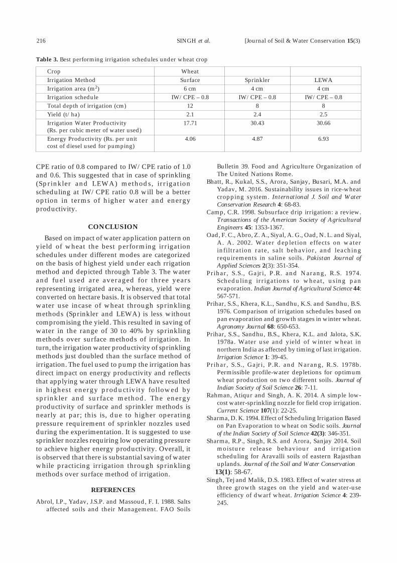
216 SINGH et al. [Journal of Soil & Water Conservation 15(3)
CPE ratio of 0.8 compared to IW/CPE ratio of 1.0and 0.6. This suggested that in case of sprinkling(Sprinkler and LEWA) methods, irrigationscheduling at IW/CPE ratio 0.8 will be a betteroption in terms of higher water and energyproductivity.
CONCLUSION
Based on impact of water application pattern onyield of wheat the best performing irrigationschedules under different modes are categorizedon the basis of highest yield under each rrigationmethod and depicted through Table 3. The waterand fuel used are averaged for three yearsrepresenting irrigated area, whereas, yield wereconverted on hectare basis. It is observed that totalwater use incase of wheat through sprinklingmethods (Sprinkler and LEWA) is less withoutcompromising the yield. This resulted in saving ofwater in the range of 30 to 40% by sprinklingmethods over surface methods of irrigation. Inturn, the irrigation water productivity of sprinklingmethods just doubled than the surface method ofirrigation. The fuel used to pump the irrigation hasdirect impact on energy productivity and reflectsthat applying water through LEWA have resultedin highest energy productivity followed bysprinkler and surface method. The energyproductivity of surface and sprinkler methods isnearly at par; this is, due to higher operatingpressure requirement of sprinkler nozzles usedduring the experimentation. It is suggested to usesprinkler nozzles requiring low operating pressureto achieve higher energy productivity. Overall, itis observed that there is substantial saving of waterwhile practicing irrigation through sprinklingmethods over surface method of irrigation.
REFERENCES
Abrol, I.P., Yadav, J.S.P. and Massoud, F. I. 1988. Saltsaffected soils and their Management. FAO Soils
Bulletin 39. Food and Agriculture Organization ofThe United Nations Rome.
Bhatt, R., Kukal, S.S., Arora, Sanjay, Busari, M.A. andYadav, M. 2016. Sustainability issues in rice-wheatcropping system. International J. Soil and WaterConservation Research 4: 68-83.
Camp, C.R. 1998. Subsurface drip irrigation: a review.Transactions of the American Society of AgriculturalEngineers 45: 1353-1367.
Oad, F. C., Abro, Z. A., Siyal, A. G., Oad, N. L. and Siyal,A. A. 2002. Water depletion effects on waterinfiltration rate, salt behavior, and leachingrequirements in saline soils. Pakistan Journal ofApplied Sciences 2(3): 351-354.
Prihar, S.S., Gajri, P.R. and Narang, R.S. 1974.Scheduling irrigations to wheat, using panevaporation. Indian Journal of Agricultural Science 44:567-571.
Prihar, S.S., Khera, K.L., Sandhu, K.S. and Sandhu, B.S.1976. Comparison of irrigation schedules based onpan evaporation and growth stages in winter wheat.Agronomy Journal 68: 650-653.
Prihar, S.S., Sandhu, B.S., Khera, K.L. and Jalota, S.K.1978a. Water use and yield of winter wheat innorthern India as affected by timing of last irrigation.Irrigation Science 1: 39-45.
Prihar, S.S., Gajri, P.R. and Narang, R.S. 1978b.Permissible profile-water depletions for optimumwheat production on two different soils. Journal ofIndian Society of Soil Science 26: 7-11.
Rahman, Atiqur and Singh, A. K. 2014. A simple low-cost water-sprinkling nozzle for field crop irrigation.Current Science 107(1): 22-25.
Sharma, D. K. 1994. Effect of Scheduling Irrigation Basedon Pan Evaporation to wheat on Sodic soils. Journalof the Indian Society of Soil Science 42(3): 346-351.
Sharma, R.P., Singh, R.S. and Arora, Sanjay 2014. Soilmoisture release behaviour and irrigationscheduling for Aravalli soils of eastern Rajasthanuplands. Journal of the Soil and Water Conservation
13(1): 58-67.Singh, Tej and Malik, D.S. 1983. Effect of water stress at
three growth stages on the yield and water-useefficiency of dwarf wheat. Irrigation Science 4: 239-245.
Table 3. Best performing irrigation schedules under wheat crop
Crop WheatIrrigation Method Surface Sprinkler LEWAIrrigation area (m2) 6 cm 4 cm 4 cmIrrigation schedule IW/CPE – 0.8 IW/CPE – 0.8 IW/CPE – 0.8Total depth of irrigation (cm) 12 8 8Yield (t/ha) 2.1 2.4 2.5Irrigation Water Productivity 17.71 30.43 30.66(Rs. per cubic meter of water used)Energy Productivity (Rs. per unit 4.06 4.87 6.93cost of diesel used for pumping)

July-September 2016] IRRIGATION WATER MANAGEMENT 217
Singh, S.R., Singh, A. K., Islam, A. and Bharali, M.A.2004. Low Energy Water Application Device,Technical Bulletin No – R-11/PAT-3. ICAR ResearchComplex for Eastern Region, Patna, Bihar, India.
Singh, A.K., Rahman, A., Sharma, S.P., Upadhyaya, A.and Sikka, A.K. 2008. Small Holders’ Irrigation-Problems and Options. Water Resources Management23:289-302.
Singh, A. K., Sharma, S.P., Upadhyaya, A., Rahman, A.and Sikka, A.K. 2010. Performance of Low EnergyWater Application Device. Water ResourcesManagement 24:1353-1362.
Singh, A.K., Islam, A., Singh, S.R., Upadhyay, A. andSikka, A.K. 2015. Low Energy Water Application
(LEWA) device: Concept and applications. Journalof Soil and Water Conservation 14(4): 344-351.
Singh, A. K., Verma, C. L., Singh, Y. P., Bhardwaj, A. K.and Singh, D. 2014. Water and energy use patternby different irrigation systems in Wheat underpartially reclaimed sodic soils. Journal of Soil andWater Conservation 13(3): 245-250.
Singh, A. K., Verma, C. L., Singh Y. P., Bhardwaj A. K.,Arora, Sanjay and Singh, D. 2016. Irrigation waterand pumping energy use trends in rice (Oryza sativaL.) under varying irrigation regimes in partiallyreclaimed sodic soils. Journal of Soil and WaterConservation 15(1): 52-57.

218 KUMAR et al. [Journal of Soil & Water Conservation 15(3)
Journal of Soil and Water Conservation 15(3): 218-225, July-September 2016ISSN: 022-457X
Geospatial technology in soil resource inventory andland capability assessment for sustainable development –
Wayanad district, Kerala
Y. SURESH KUMAR1, N. S. GAHLOD2 and V. S. ARYA3*
Received: 19 June 2016; Accepted: 19 August 2016
ABSTRACT
Geospatial technology has opened new vistas for natural resources mapping and their management.It has been widely used for soil resources inventory and generation of spatial and temporalinformation for sustainable landuse plan at a specific scale. The present study was undertaken toidentify the different physiographic situations, landforms and soil resources to assess the chemicaland physical inherent soil properties, topography, slope, climate and land use as an external landfeature. IRS-ID (LISS-III) satellite data was used to delineate different physiographic units usingimage interpretation keys on 1:50,000 scale alongwith exhaustive ground truthing. The soils wereclassified on the basis of Soil survey and laboratory data. The generated spatial and non-spatialdata was integrated in the Geographic Information System (GIS) environment and various thematiclayers were derived to prepare land capability map of the district. The main physiographic unitsidentified in the study area were undifferentiated hill slopes, pediments, pediplains and narrowriver valleys. The soils found in the area were moderately deep to deep, fine loamy to fine texturedon hill side slopes occupying 71.6% area, deep to very deep, fine loamy to fine textured on pedimentscovering 7.8% area and very deep, fine to coarse loamy soils, mostly aquic in nature in narrow rivervalleys with 19.3% area of district and classified as Entisols, Inceptisols and Mollisols. It was foundthat soils of the valley fall in land capability class- II, pediments in class- III and hills in the range ofIV to VIII.
Key words: Geospatial, GIS, IRS-ID, LISS-III, Pediment, Land capability
1,2Assistant Soil Survey Officer, Soil & Land Use Survey of India; 3Chief Soil Survey Officer, Soil& Land Use Survey of India, New Delhi; *Corresponding author Email: [email protected]
INTRODUCTION
Soil is a life supporting system upon whichcivilization have been dependent and intensificationof agriculture on land used for farming system inlast few decades, a sequence of change hasimmerged in traditional resource use due topopulation pressure and increasing demand forfood, fodder, fuel etc. in the every region. Thusmanagement of natural resources, specially becomeessential for variety of purposes viz. command areadevelopment, soil conservation in catchment areas,sustainable agriculture, watershed management,reclamation of degraded lands etc. Soil resourceinventory provides an insight into the potentialitiesand limitation of soil for its effective exploitationand interpretation for multifarious land uses.Understanding the soil distribution patterns inrelation to landscape attributes is seen as a step to
improve the accuracy of soil mapping in remotelocations. However, this variation is not randombecause the properties of soil vary from place toplace. Natural soil bodies are the result of climateand living organisms acting on parent material,with topography or local relief exerting a modifyinginfluence with time required for soil-formingprocesses to act (Soil Survey Division Staff, 1993).
Topography is often used in soil distributionstudies for prediction of soil type as because it hasa overwhelming influences on most of the soilforming factors (Jenny, 1980; Pennock et al., 1987;Moore et al., 1993; McKenzie et al., 2000; Ballabio,2000). Soil physic-chemical properties are one ofthe important information categories forappropriate land management and environmentalmodeling (Florinsky et al., 2002; Herbst et al., 2006;Ziadat, 2007; Dhale et al., 2015).
July-September 2016] GEOSPATIAL TECHNOLOGY IN SOIL RESOURCE INVENTORY 219
The soil can be characterized by its structure,color, consistence, texture, and abundance of roots,cracks, and carbonates. These characteristics allowscientists to interpret how the soil ecosystemfunctions and make recommendations for soil usethat have a minimal impact on the ecosystem. Itcan help them to determine the types of vegetationand land use best suited to a location (Globe, 2005).Characterization of soils is fundamental to all soilstudies, as it is an important tool for soilclassification, which is done based on soil properties.Soil characterization also helps to document soilproperties at research sites, which is essential forthe successful transfer of research results to otherlocations (Buol et al ., 2003). Natural soilphenomenon and conservation processes playcrucial role in designing sustainable land use plan(Joseph et al., 2016).
Remote Sensing has emerged as an importanttool in soil resource inventory and generation ofinformation on spatial and temporal basis whichhelps in evolving the optimum landuse plan forsustainable development at specific scale. Thesatellite data is interpreted as a function of soilproperties and soil units delineated with respectto image characteristics and correlated withlandform-topography information from Survey ofIndia Toposheets and geology information fromdistrict resource map geological survey of India.The dynamic inter-relationship betweenphysiography and soils is utilized for deriving soilinformation from satellite data (Kudrat et al., 1992).In interpretation of satellite image for soil mappingproper identification of land type, drainage pattern,and drainage condition, vegetation, land use, slopeand relief is very essential (Dwivedi, 2001).
Wayanad district stands on the southern tip ofthe Deccan plateau and Chembra Peak [2,100metres (6,890 ft)], Banasura Peak [2,073 metres(6,801 ft)], Brahmagiri [1,608 metres (5,276 ft)] aresome of the important mountains in the district.The entire area of district is drained by Kabini Riverand its three tributaries viz., the Panamaram,Mananthavady, and Kalindy rivers. Agriculturallythe district is characterized by the cultivation ofperennial plantation crops and spices. The majorplantation crops include coffee, tea, pepper,cardamom and rubber. A recent increase in the areaunder coconut cultivation is noticed in the lowerelevations along with paddy.
In the present study an attempt has been madeto generate digital soil map exhibiting distributionof different soils types based on their inherentmorphological properties, correlated with
laboratory analysis and were classified based onComprehensive System of Soil Classification (SoilTaxonomy, 2010). It also provides information tothe land capability and appropriate soil and landmanagement system which is essential todetermine best land use for sustained cropproduction in district.
MATERIALS AND METHODS
Description of the Study areaWayanad district forms part of the Western
Ghats occupying an area of 2,13,939 hectaresgeographically located between 110 27' to 150 58'North latitude and 750 47' to 700 27' East longitudeand it is bounded on the south by Malappuram,west by Kozhikode and Kannur district of KeralaState, north by Coorg district of Karnataka, eastby Nilgiris and Mysore districts of Tamil Nadu andKarnataka State respectively. Wayanad district fallsin the Agro-climatic Zone-XII (West Coast Plains& Ghat Region) with large area covered underforest. It has a large amount of dry and moistdeciduous forest. Wayanad is home to endangeredspecies. The climate of the district is almost coolthroughout the year except for April and Maywhich reaches the peak summer; a maximum to310 is rarely reached, with the temperatureremaining around 290 and hot breezes in summer.In the monsoon season it rains heavily almost withannual average rain of 3200 mm. The winters arecold in some areas of northern part of the districtwith January as the coldest month. The locationmap is shown in Fig. 1.
Soil Resource Characterization and SamplingDigital data of IRS-1D -LISS III (Spatial
resolution of 23.5 m) was used to extract thedifferent types of soils association information onthe base map derived from Survey of Indiatoposheet on 1:50K, from which soil map wasprepared by incorporating morphologicalcharacteristics and laboratory analysis data of soilprofile. The methodology followed for extractionof information from satellite data is essentially ofstandard monoscopic visual interpretation basedon tone, texture, shape and size. The topographicfeatures (i.e. surface elevation, slope, aspect, relief);major physiographic units and land use (i.e. forest,agriculture, plantation, waste land, and scrub) wereextracted from Survey of India Toposheets of 1:50Kscale. The origin of soil deposits were extractedfrom geological map of the district of GeologicalSurvey of India. The data extracted from both the

220 KUMAR et al. [Journal of Soil & Water Conservation 15(3)
in physiographic unit, parent material type, landuse land cover and slope map. Each map representsthe factors which influence soil formation.Representative soil profiles were selected torepresent delineated soil mapping units; themorphological description of these profiles wascarried out according to the guidelines of SoilSurvey Manual developed by Soil and Land UseSurvey of India AISLUS, 1970. Soil site informationwas also recorded. Horizon wise soils sampleswere collected for laboratory analysis physical andchemical properties.
Laboratory AnalysisAll Laboratory analyses were done following the
procedures in Soil laboratory manual prepared byAISLUS (2000). The soil samples were air-dried andground to pass a 2-mm sieve and before analysis.Soil texture was determined by Bouyoucoshydrometer method. The pH and electricalconductivity of the soils were measured in water(1:2.5 soil:water ratio). Organic carbon content ofthe soil was determined following the wetcombustion method of Walkley and Black (1934).Exchangeable cations and the cation exchangecapacity (CEC) of the soil were determinedfollowing the 1 N ammonium acetate (pH 7)method. The exchangeable K and Na in the extractwere measured by flame photometer. Calcium andmagnesium were measured using EDTA titrationmethod. The available potassium was determinedby Morgan’s extraction solution and potassium inthe extract was measured by flame photometer.Water holding capacity was carried out by Keen RBox Method; Moisture equivalent at 1/3 and 15 barwas carried out by pressure plate apparatus.
Taxonomic Soil Classification and Soil Map GenerationA taxonomic soil classification is directly based
on soil characteristics where as capabilityclassification is an interpretive classification basedon effects of combination of climate and permanentsoil characteristics on risks of soil damage,limitations in use, productive capacity and soilmanagement requirements. The ComprehensiveSystem of Soil Classification (Soil Taxonomy, 2010)was followed to classify the different soils of thedistrict to correlate the physiographic andtaxonomic units. Soils of the district were classifiedunder orders Entisols, Inceptisols and Mollisols.All theses maps were transferred to GISenvironment, overlaid and used as base map forfield survey to incorporate the results with fieldobservations. The soil boundary was delineated
Fig. 1. Location Map of Wayanad District, Kerala
sheets were converted into defined soil units byusing satellite imagery and were verified byground truthing through field observations andsoil sample collection. Based on variations of thesefactors, sample strips have been selected fordetailed morphological study of the soils.
Soil profiles were studied based on variations

July-September 2016] GEOSPATIAL TECHNOLOGY IN SOIL RESOURCE INVENTORY 221
based on the boundary inferred by combination ofdifferent layers representing soil forming factorsthat were used in as base map. The polygonsrepresenting similar physiographic unit, parentmaterial, slope and vegetation cover was put undersame soil type which is confirmed by imagecharacteristics and field survey. Different kind ofsoil can be expected if there is any change of thesefactors. The soil map was used for land evaluation.The spatial data were analysed for interpretingcapability class of soils based on theircharacteristics and limitations to evaluate theirpresent and future potentialities. The landcapability map was generated for planners to beused as a vital input to prepare a strategic planningfor effective and efficient decision making.
RESULTS AND DISCUSSION
Physiography and SoilsAccording to the climatic data the soil
temperature regime of the district is ‘Isohyperthermic’and soil moisture regime is ‘Udic’ in general and“Aquic” in lower valleys.
Based on the Satellite Imagery, Survey of India
Toposheets and field checks the physiography ofthe district was identified. The obtained resultsrevealed that the major physiographic unites in thedistrict area comprises of undifferentiated hillsslopes dominating most of the district area (71percent) followed by pediments, undulatingpediplain and valleys.
The major portion of the study area is underforest and plantations of tea, coffee, rubber withcoconut in patches and paddy in the lower valleysand pediplains. The soils associations developedon the hills and pediments to undulatingpediplains are deep to very deep and that in valleysare very deep soils. The digital soil map with soilmapping units is presented in the Fig. 2.
The undifferentiated hill slopes under variousland use are soil associations of least or partiallydeveloped, moist, gravelly fine loamy to loamyskeletal soils belongs to Entisol (Typic Udorthent)supporting forest vegetation on higher slopinglandforms and freely drained, deep to very deephaving moderate available moisture. These soilsare associated with deep to very deep, fine loamyto fine and gravelly fine textured soils of Inceptisol(Typic/Oxic Dystrudepts, Typic/dystric
Fig. 2. Soil Map of Wayanad District, Kerala
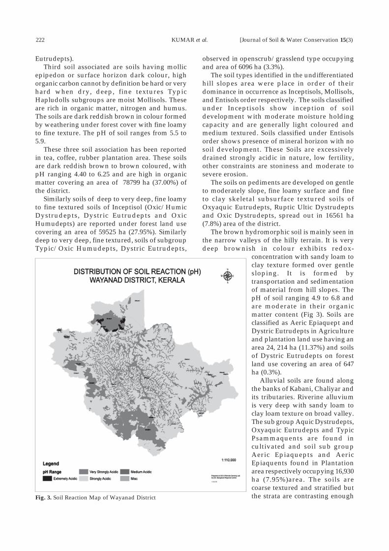
222 KUMAR et al. [Journal of Soil & Water Conservation 15(3)
Eutrudepts).Third soil associated are soils having mollic
epipedon or surface horizon dark colour, highorganic carbon cannot by definition be hard or veryhard when dry, deep, fine textures TypicHapludolls subgroups are moist Mollisols. Theseare rich in organic matter, nitrogen and humus.The soils are dark reddish brown in colour formedby weathering under forest cover with fine loamyto fine texture. The pH of soil ranges from 5.5 to5.9.
These three soil association has been reportedin tea, coffee, rubber plantation area. These soilsare dark reddish brown to brown coloured, withpH ranging 4.40 to 6.25 and are high in organicmatter covering an area of 78799 ha (37.00%) ofthe district.
Similarly soils of deep to very deep, fine loamyto fine textured soils of Inceptisol (Oxic/HumicDystrudepts, Dystric Eutrudepts and OxicHumudepts) are reported under forest land usecovering an area of 59525 ha (27.95%). Similarlydeep to very deep, fine textured, soils of subgroupTypic/Oxic Humudepts, Dystric Eutrudepts,
observed in openscrub/grasslend type occupyingand area of 6096 ha (3.3%).
The soil types identified in the undifferentiatedhill slopes area were place in order of theirdominance in occurrence as Inceptisols, Mollisols,and Entisols order respectively. The soils classifiedunder Inceptisols show inception of soildevelopment with moderate moisture holdingcapacity and are generally light coloured andmedium textured. Soils classified under Entisolsorder shows presence of mineral horizon with nosoil development. These Soils are excessivelydrained strongly acidic in nature, low fertility,other constraints are stoniness and moderate tosevere erosion.
The soils on pediments are developed on gentleto moderately slope, fine loamy surface and fineto clay skeletal subsurface textured soils ofOxyaquic Eutrudepts, Ruptic Ultic Dystrudeptsand Oxic Dystrudepts, spread out in 16561 ha(7.8%) area of the district.
The brown hydromorphic soil is mainly seen inthe narrow valleys of the hilly terrain. It is verydeep brownish in colour exhibits redox-
concentration with sandy loam toclay texture formed over gentlesloping. It is formed bytransportation and sedimentationof material from hill slopes. ThepH of soil ranging 4.9 to 6.8 andare moderate in their organicmatter content (Fig 3). Soils areclassified as Aeric Epiaquept andDystric Eutrudepts in Agricultureand plantation land use having anarea 24, 214 ha (11.37%) and soilsof Dystric Eutrudepts on forestland use covering an area of 647ha (0.3%).
Alluvial soils are found alongthe banks of Kabani, Chaliyar andits tributaries. Riverine alluviumis very deep with sandy loam toclay loam texture on broad valley.The sub group Aquic Dystrudepts,Oxyaquic Eutrudepts and TypicPsammaquents are found incultivated and soil sub groupAeric Epiaquepts and AericEpiaquents found in Plantationarea respectively occupying 16,930ha (7.95%)area. The soils arecoarse textured and stratified butthe strata are contrasting enoughFig. 3. Soil Reaction Map of Wayanad District

July-September 2016] GEOSPATIAL TECHNOLOGY IN SOIL RESOURCE INVENTORY 223
to cause water perching or to have marked impacton permeability. Draining these soils can createmoisture stress because there is no buffering effecton moisture content.
Land capability assessment: The spatialanalyses technique was adapted to evaluate theagricultural land capability in the study area. Thedifferent landforms were identified which wasused as a base to delineate soil boundaries toidentify different soil types and soil map layer wasproduced using ArcGIS. The attributed data of landslope, soil organic matter, pH, textural class, soildepth, acidity, CEC, Soil erosion and drainagecondition were linked with the units of the digitised
soil map in GIS. The incorporated attributes wereused to generate thematic layers of spatialdistribution of the above mentioned characteristicsand properties. The produced layer includesinformation on capability class and spatialdistribution for the soil characteristics. The dataobtained indicated that the main limiting factorsin the district were slope, terrain, soil texture,drainage, erosion and CEC.
The land capability classification for the soils ofthe district has been interpreted for agriculturepurpose and is depicted in the Table 1. Soilsdeveloped on valleys and lower plains have beenclassified as Class II which requires careful soil
S. Land Soil Units Associated Recommendations Area AreaNo. Capability problem (ha) (%)
Class1. Class II Valleys and
Lower Plains -underAgriculture &Plantation
Stratified soilprofile. Prone toWater-logging /Flooding. Neutral toacidic reaction (pH).Low base saturation.Shallow groundwater.
Suitable for cultivation of Paddy, Coconut,Coffee, Tapioca, Pepper, Tea, Cocoa.Adoption of mechanized cultivation.Cultivation of pulses in summer fallowslivelihood support through livestock andfisheries. Popularization of organicfarming and certification. Soil test basedcomprehensive nutrient management.Lime application in soil.
41143 19.3
2. Class III Pediments -Plantations
Gentle to moderateslope. Acidic innature. Low basesaturation
Rejuvenation of existing homesteads.Multilayered and mixed farmingsystems.Popularization of organic farmingand certification.Lime application in soil.
16561 7.8
3. Class IV Hills (steepslopes) -Plantations
Acidic in nature.Low base saturation.
Renovation &strengthening of waterharvesting and storagestructures.Cultivation of cool seasonvegetables.Lime application in soil
36391 17.1
4. Class VI Hills (steepslopes) - OpenScrub
Deforestation. Proneto erosion. Acidicnature of soils.
Soil & water conservation throughcontour/staggered trenching works.Construction of terrace support wall.Pasture development.
271 0.1
5. Class VII Hills (verysteep slopes) -Plantations
Weak soildevelopment Acidicnature of soils.Prone to erosion
Cultivation of medicinal plants. Formationof bench terraces with vegetative barrier.Contour/staggered trenching works andformation of bench terraces.
42602 20.0
6. Class VIII Hills (very steepslopes) - Openscrub /grass
Deforestation. Proneto erosion. Acidicnature of soils.
Treatments of land slip areas withvegetative barrier. Afforestation ofdenuded forest land. Pasture development.
6715 3.2
7. Forest (F) Hills(steep tovery steep slopes),Pediments &Valleys underForest
Deforestation. Proneto erosion. Acidicnature of soils.
Afforestation of denuded forest land.Contour/staggered trenching works andformation of bench terraces. Fire linescrapping, to set up fire protection tower.
66848 31.4
Table 1. Land capability class of Wayanad District
8. Misc. ROC,Habitation,Water bodiesetc.
- - 2408 1.1
Total 212939 100.0

224 KUMAR et al. [Journal of Soil & Water Conservation 15(3)
management to prevent deterioration as these soilsare under plantation and paddy and hadlimitations of slope, moderate susceptibility towind or water erosion, drainage overflow andwetness.
Soil developed on pediments under plantationsare classified as Class III with major limitation ofmoderately steep slopes, high susceptibility towater erosion, frequent over flow and low tomoderate water holding capacity. Soils under thisclass require proper drainage that improves thestructure and tilth of the soils. Soils developed onhills with steep slopes under plantations mainlyof rubber have been classified as Class IV havingvery severe limitations that restrict the choice ofplants and requires very careful management. Themajor limitations for this class are steep slopes,erosion. The generated digital land capability mapis presented in Fig. 4.
CONCLUSION
Soil Taxonomy was guided by morphogeneticprinciples but, wherever possible, the parametersthat define taxa or classes are important to soil uses.
Thus, useful interpretations can be inferred fromsoil taxa names. Most of the managementinformation is presented at the level of soil seriesor its phases. Because the system is morphogenetic,surface soil characteristics, which are so critical tocrop performance, receive least attention. In thisstudy attempt has been made to developsustainable land use plan based on soil and landproperties along with taxonomic class of soil seriesIt has also confirmed that the physiographicposition, Land use and elevation play an importantrole in the variation in soil properties such asorganic carbon, depth, texture, structureirrespective of landscape or parent material, whichis a key factor for sustainable land use planning insuch least accessible mountainous area.
ACKNOWLEDGEMENT
Authors want to acknowledge their sincerethanks to the Natural Resource Management(NRM) division, Department of Agriculture,cooperation and farmers welfare, Ministry ofAgriculture and farmers welfare, Government ofIndia for providing the facility for analysis of data

July-September 2016] GEOSPATIAL TECHNOLOGY IN SOIL RESOURCE INVENTORY 225
and financial assistance for presenting the data forthe benefit of user community.
REFERENCES
AIS & LUS 1970. Soil Survey Manual, All India Soil &Land Use Survey; IARI buildings, New Delhi 110012.
AIS & LUS 2000. Soil Laboratory Manual, All India Soil& Land Use Survey; IARI buildings, New Delhi-110012.
Ballabio, C. 2009. Spatial prediction of soil propertiesin temperate mountain regions using support vectorregression. Geoderma 151: 338–350.
Boettinger, J. L. 2010. Environmental covariates fordigital soil mapping in the western USA :17–27. InJ.L. Boettinger, D.W. Howell, A. C. Moore, A. E.Hartemink and S. Kienast-Brown,(eds.). Digital SoilMapping: Bridging Research, EnvironmentalApplication, and Operation. Springer ScienceBusiness Media. Dordrecht, the Netherlands.
Buol, S. W., R. J. Southard, Graham, R. C. and McDaniel,P. A. 2003. Soil Genesis and Classification, Iowa StatePress, pp. 512.
Dhale, S.A., Meena R. L. and Arya, V. S. 2016.Assessment of soil physic-chemical properties forscientific land use planning in Palakkad district ofKerala using remote sensing and GIS techniques.Kerala state Land Use Board. National Seminar 2016-Land Use Planning. Pp. 131-135.
Dwivedi, R.S. 2001. Soil resource mapping: A remotesensing perspective. Remote Sensing Reviews 20: 89–122.
Florinsky, I. V., Eilers, R. G., Manning G. R. and Fuller,L. G. 2002. Prediction of soil properties by digitalterrain modeling. Environmental Modelling & Software17: 295–311.
Globe. 2005. Soil Characterization Protocol, Field Guide.https://core.ac.uk/download/pdf/5220603.pdf
Herbst, M., Diekkrüger B. and Vereecken, H. 2006.Geostatistical co-regionalization of soil hydraulicproperties in a micro-scale catchment using terrainattributes. Geoderma 132: 206–221.
Jenny, H. 1980. The Soil Resources: Origin and Behavior.Springer-Verlag. New York, NY, USA.: pp. 377.
Joseph A.W.M., Meena, R. L. and Arya, V. S. 2016. Landresource inventory for evaluation of land cspsbilityand land use planning in Palakkad district of Kerlausing remote sensing and GIS techniues. Kerala stateLand Use Board. National Seminar 2016- Land UsePlanning:92-95.
Kudrat, M., Tiwari, A. K., Saha, S. K. and Bhan, S. K.1992. Soil resource mapping using IRS 1A LISS-IIdigital data — A case study of Kandi area adjacentto Chandigarh, India. Int. J. Remote Sensing 13(17):3287–3302.
McKenzie, N. J., Gessler, P. E., Ryan, P.J. and O’Connell,D.A. 2000. The role of terrain analysis in soilmapping. : 245–266. In J. P. Wilson and J. C. Gallant,(eds.) Terrain analysis: Principles and application. JohnWiley & Sons. New York, NY, USA.
Moore, L. D., Gessler, P. E., Nielsen, G. A. and Peterson,G. A. 1993. Soil attribute prediction using terrainanalysis. Soil Science Society of America Journal 57: 443–452.
Pennock, D. J., Zebarth, B. J. and Jong, E. D. 1987.Landform classification and soil distribution inhummocky terrain, Saskatchewan; Canada. Geoderma40(3-4): 297–315.
Soil Survey Division Staff. 1993. Soil Survey Manual.United States Department of Agriculture. Washington,DC, USA, pp. 437.
Ziadat, F. M. 2007. Land suitability classification usingdifferent sources of information: Soil maps andpredicted soil attributes in Jordan. Geoderma 140:73–80.

226 PRASAD et al. [Journal of Soil & Water Conservation 15(3)
Journal of Soil and Water Conservation 15(3): 226-232, July-September 2016ISSN: 022-457X
Impact of Albizia procera benth. based agroforestrysystem on soil quality in Bundelkhand region of Central India
RAJENDRA PRASAD1*, RAM NEWAJ2, V.D. TRIPATHI3, N.K. SAROJ4, PRASHANT SINGH5,RAMESH SINGH6, AJIT7 and O.P. CHATURVEDI8
Received: 7 June 2016; Accepted: 29 August 2016
ABSTRACT
Agroforestry plays an important role in influencing soil quality indicators but their quantitativeassessment in A. procera based agroforestry system were not existing in Bundelkhand region ofCentral India. Hence, study was undertaken at Central Agroforestry Research Institute, Jhansi todevelop an additive unified Soil Quality Index (SQI) based on functional scores of soil qualityindicators comprising of soil physical, chemical and biological properties, and determine howindicators respond to different management practices. Study was conducted in a well established10 years old Albizia procera Benth. based agroforestry experiment consisting of five treatments viz.control (Pure crop), Pure tree (without inter cropping), zero pruning+ inter cropping, 50% pruning+inter cropping and 70% pruning + inter cropping. Findings revealed that maximum value of SQIwas observed for practice of zero pruning (0.54) closely followed by 50% pruning (0.53) and 70%pruning (0.52). Pure crop had the minimum SQI (0.37). Agroforestry plots viz. pure tree, zero pruning,50% pruning and 70% pruning had improved soil health to the tune of 19.7, 31.3, 31.0 and 30.0 percent, respectively, over pure crop. It has been observed that biological activities and water holdingcapacity of soil appears to be the most limiting indicators.
Key words: Indicator, Soil health, Soil quality index, Tree pruning, Semi-arid region
1,2,6 Principal Scientist, 3Research Associate, 4,5Senior Research Fellow, 8Director, ICAR-Central Agro-forestry Research Institute,Gwalior Road, Jhansi-284 003 (UP); 7Principal Scientist, ICAR-Indian Agricultural Statistics Research Institute, New Delhi-110012*Corresponding author’s email:[email protected]
INTRODUCTION
Assessment of soil quality or health inagroforestry acquires more relevance due toexpansion of area under agroforests in tropics andsub tropics, and their enhanced contributiontoward sustainability of agricultural production.In India, as per one estimate, about 25.72 millionha area has been covered under various types ofagroforestry plantations. The task force onGreening India (Anonymous, 2001) has identifieda potential of 10 million ha in irrigated lands and18 million ha in rainfed areas that could bedeveloped through agroforestry on a watershedbasis. The main driving force and objective ofcovering such large area under agroforests is to keepthe soil resource productive on sustainable basis.
Soil degradation has become a major globalissue in recent years. It has been estimated that thedegraded area increased from 10% of the world’sarable land in early 1970s (Biswas and Biswas, 1974)to 40% in early 1990 (Oldeman, 1994). In India,
nearly 188 Mha land area suffers from one or otherkind of land degradation. Various forms of soil /land degradation reduce soil’s capacity to perform.Reduction in the functional capacity of soil resultsin decline of productivity. The declining trends infood grain productivity threaten agriculturalsustainability. The concept of agriculturalsustainability expressed during last two decadesof twentieth century is being magnified in twentyfirst century because of limited arable landresources, rapid increase in population, conversionof agricultural land to other uses and persistenceof hunger and malnutrition in several regions ofthe world (Lal, 1998). Therefore, the question ofagricultural sustainability became extremelyrelevant and led to considerable interest inproductivity trends of long-term experiments (Laland Stewart, 1995). It is also emphasized thatmaintaining the quality of natural resource basewould ensure sustainability of agriculturalproduction.

July-September 2016] IMPACT OF ALBIZIA ON SOIL QUALITY 227
Assessment of soil quality depends on indicatorsthat relate to various soil functions. Depending onapproaches viz. descriptive or qualitative andquantitative soil quality assessment, the indicatorscan be observational features of soil or plantsgrowing on it, and measure of physical, chemicaland biological soil attributes. The quantitativeapproach offers greater precision but requires moreresources for doing assessment. Before selectingsoil quality indicators for assessment programme,the basic fact regarding soil to be given dueconsideration is that soil quality embraces twogeneral elements viz. i) inherent properties of soilor inherent capacity and ii) dynamic nature of soil.The inherent capacity of soil is the result of factorsof soil formation- climate, topography, vegetation,parent material and time. Attributes of inherent soilquality such as mineralogy and particle sizedistribution are almost static and show little changeover time. The dynamic nature of soil encompassesthose soil attributes that can change over relativelyshort time in response to human management.These soil attributes are referred as indicators ofsoil health. Hence, assessment of soil quality refersto assessment of dynamic soil attributes (Doran andParkin, 1994). The selected indicators of soil qualityshould have greatest sensitivity to changes in soilfunction (Andrews et al., 2004). It is emphasizedthat soil quality indicators should correlate wellwith ecosystem processes; integrate soil processes,accessible to many users and sensitive tomanagement and climate (Daran and Parkin, 1996;Sharma et al., 2010). Further, the group of indicatorsselected to measure soil functions must besufficiently diverse to represent the chemical,biological and physical properties and processesof complex system.
The overriding objective of agroforestry landuse, since its inception with establishment of WorldAgroforestry Centre in 1977, has been to developintegrated land management systems involvingtrees, crops and/ or animals, which wouldcontribute substantially to decrease deforestation,increase food production, enhance biodiversity andprotect environment (Nair, 1993). It is argued thatpresence of woody perennials in agroforestrysystem affects several bio-physical and bio-chemical processes that determine the health of soilsubstrate. The most obvious effects of trees on soilinclude amelioration of erosion primarily throughsurface litter cover and under story vegetation(Gupta and Arora, 2015); maintenance or increaseof organic matter and diversity through continuousdegeneration of roots and decomposition of litter
(Solanki and Arora, 2015); nitrogen fixation;enhancement of physical properties such as soilstructure, porosity and moisture retention due toextensive root system and the canopy cover; andabsorb and recycle nutrients in the soil that wouldotherwise be lost through leaching (Sanchez, 1987).Although soil conservation for restoring qualityand health of degraded soil has been advocatedas primary goal of agroforestry (Young, 1989), theempirical estimates of accrued benefits are lackingdue to temporal and spatial complexity ofagroforestry systems and soil resource dynamics.
Use of soil quality index (SQI) value based onsummarized soil properties to assess soil qualityof agricultural and forest ecosystems is wellestablished, however, the systematic informationon use of a unified value of SQI to assess impact ofvarious agroforestry systems on soil quality islacking. Thus, development and application of asoil quality index for evaluation of changes in soilquality caused due to agroforestry practices isneeded. Further it is hypothesized that variousagroforestry systems being advocated areproductive, remunerative and environmentfriendly; and to prove this hypothesis, it is essentialto assess impact of various agroforestrymanagement practices on soil quality. Therefore,the present study was conducted to assess changesin soil quality indicators and soil quality index dueto pruning management practices in Albizia procerabased agroforestry system in semi arid region ofBundelkhand, Central India.
MATERIALS AND METHODS
Site description: The study was carried out atthe farm of ICAR-Central Agroforestry ResearchInstitute (CAFRI), Jhansi during 2010. The soil ofthe experimental farm is inter-mixed black and redsoil, which represent parawa group of soil ofBundelkhand region covered under the order ofAlfisol. The CAFRI farm is situated at 25o 27’ Northlatitude and 78° 35’ East longitude, 271 metersabove mean sea level in the semi-arid tract ofcentral plateau of India. Annual rainfall rangesfrom 700-1150 mm with a mean value of 958 mmof which, about 80% is received during southwestmonsoon. The potential evapo-transpiration isquite high in the range of 1400-1700 mm withmoisture index value of - 40 to -50. The pattern ofthe rainfall is highly erratic and more than 90 percent of the total rainfall occurs within 10 weeksbetween July to mid September accompanied byintermittent long dry spells. The entire rainfall is

228 PRASAD et al. [Journal of Soil & Water Conservation 15(3)
received in less than 50 rainy days. Winter showersare rare and uncertain. The frequent drought occursin entire regions. Usually, monsoon commences bythe last week of June but sometimes delayed to thefirst week of July. The active monsoon oftenwithdraws up to the mid of September or the endof August. Mean annual temperature of the Jhansiis generally high with high degree of variationbetween maximum (39.80C in June) and minimum(5.80C in January) temperatures. Sometimesmaximum temperature in the summer months ofMay and June touches 480C, which is the peak ofsummer season.
Experimental design and management: Thepresent study was conducted in a well established10 years old A. procera based agroforestry trialconsisting of five treatments viz. control (Purecrop), Pure tree (without inter cropping), zeropruning + inter cropping, 50% pruning + intercropping and 70% pruning + inter cropping during2010. The trial was laid out in completelyrandomized block design (CRBD) with threereplications. Trees planted at 8x4 m spacing wereintercropped with wheat in winter season. Thepruned biomass from 50% and 70% pruningtreatment was added in soil as green manure inthe month of October, at least one month beforesowing of wheat as intercrop. Levels of pruningwere based on a percentage of green crown lengthand pruning was done by cutting lower branchesfrom stem or parent branch. Branches were takenout for using as fuel and green twigs/foliage wasincorporated in the soil as green manure. Greenbiomass in the tune of 1.99 t/ha and 2.27 t/ha wasadded in 50% and 70% pruning treatments,respectively. Wheat (Triticum aestivum L. emend.)variety HD 2189 was grown as an inter crop.Standard package of practices of wheat cultivationwere followed.
Soil sampling and analyses for soil healthindicators: Rrepresentative soil samples weredrawn (0-30cm depth) from all treatment plotsbefore sowing of wheat. The soil samples were airdried and sieved to pass through a 2 mm-sieve.For the determination of bulk density, soil coreswere collected. Soil samples collected wereseparately analyzed for physical, chemical andbiological properties as listed below. Bulk density(BD) was determined from the soil cores using theprocedure given by Veihmeyer and Hendrickson(1948), and porosity was derived from BD usingthe following formula: porosity (P) = [1- (BD/PD)]*100, where PD is the particle densitydetermined using a Keen Raczkowald (KR) box
(Baruah and Barthakur, 1999). KR box is a circularbrass box having an internal diameter of 5 cm anda height of 1.6 cm with perforated bottom havingnumerous holes of 0.75 mm diameter spaced at 4mm apart. Maximum water holding capacity(WHC) was determined by equilibrating the soilwith water through capillary action in a KR box(Baruah and Barthakur, 1999). Soil pH and EC weredetermined at 1:2.5 soil–water ratio using a glasselectrode and conductivity bridge, respectively.Cation exchange capacity (CEC) was measured bythe sodium saturation method (Jackson, 1973). Soilorganic carbon (SOC) was determined bydichromate oxidation (Walkley and Black, 1934)and available N by the alkaline potassiumpermanganate distillation method (Subbiah andAsija, 1956). Available phosphorus (P) in soil wasdetermined by extracting samples with 0.5 MNaHCO3, and determining P colorimetrically usingmolybdate (Olsen et al., 1954). Available potassiumwas determined using 1N ammonium acetateextraction followed by emission spectrometry(Jackson, 1973). Microbial biomass carbon wasmeasured by the fumigation extraction method(Jenkinson and Ladd, 1981). Soil dehydrogenasewas determined using the method of Klein et al.(1971).
Soil quality index (SQI) calculationAnalysis of variance (ANOVA) was performed
to determine the effects of pruning treatments inAgroforestry systems on soil quality parameters.For calculating soil quality index (SQI) 12 soilquality indicators viz., bulk density, water holdingcapacity (WHC), porosity, pH, EC, SOC, CEC,available N, P and K; microbial biomass anddehydrogenase activity were as used asparameters. The minimum and maximumthreshold values for each indicator are based onthe range of values measured from agroforestrysystems and on critical values in the literature.After setting thresholds, the soil parameter valuesrecorded under Albizia procera based agroforestrysystem were transformed in to unit less scores(between 0 and 1) and three types of scoringfunctions viz. “More is better”, “Less is better” and“Optimum” were generated following Karlen andStott (1994). Such scoring curves were also usedby Masto et al. (2007).
Linear scoring function:LSF (Y) = (x-s)/ (t-s)………(1)Y = 1-[(x-s)/ (t-s)]………… (2)Where, Y is the linear score, x is the soil
parameter value, s and t are the lower and upper

July-September 2016] IMPACT OF ALBIZIA ON SOIL QUALITY 229
threshold values. Equation 1 is used for “More isbetter” scoring function, Equation 2 for “Less isbetter” and combination of both for “Optimum”scoring function (Fig. 1). If the calculated score is> 1.0, it was considered as 1.0. The individual scoreswere added up to obtain unified soil quality Index(SQI) as below:
SQI = i=1∑n Si/n
Where, S denotes linear scores of observed soilquality indicator, n is the number of total indicatorincluded in the index.
RESULTS AND DISCUSSION
Effect of pruning management on soil quality indicatorsThe data relating to mean values of all physical,
chemical and biological parameters of soil underdifferent pruning management regimes of A.procera based agroforestry system have beenpresented in Table 1. As revealed from data,pruning of trees significantly affected all studiedsoil health indicators except water holdingcapacity, EC and available K. Maximum bulkdensity was observed in pure tree plot whileminimum in 50 % pruning. In comparison to purecrop plot bulk density was reduced in allagroforestry plots viz. zero, 50 % and 70 % pruningplots. Maximum porosity was found in 50 %pruning plot while minimum in pure crop. Ingeneral, there was increase in porosity inagroforestry plots subjected to pruningmanagement in comparison to pure crop and puretree plot. As compared to pure crop, soil pH wasreduced in agroforestry plots. Maximum soilorganic carbon was found in zero pruning plot
while minimum in pure crop. There was significantincreased in SOC in all agroforestry plots ascompared to pure crop. Maximum CEC was foundin 70 % pruning plots while minimum in pure cropplot. Pruning management in agroforesty plotsignificantly increased the CEC. In comparison topure crop plot, available N increased inagroforestry plot with maximum in 50 % pruning.However, maximum value of available P wasobserved in zero pruning plot with minimum inpure crop. Maximum microbial biomass wasobserved in 70% pruning while minimum in purecrop plot. It increased in agroforestry plot withincreasing levels of pruning from zero to 70%.Maximum dehydrogenase activity was found inpure tree plot and minimum in pure crop. Ingeneral, all agroforestry plots had moredehydrogenase activity than that in pure crop.
The practice of agroforestry for 10 years and treepruning management brought a significantimprovement in physical, chemical and biologicalparameters of soil, which may be due to increasein SOC, recycling of nutrients through leaf litterand favorable conditions for bio-chemicalprocesses (Sanchez, 1987; Nair, 1993). Increase inSOC in agroforestry plots over pure crop might bedue to comparatively resistant organic carbonadded through tree pruning/ leaf letter and moreroot biomass yielded by trees (Ram Newaj et al.,2007; Prasad et al., 2015). Maximum available P inzero pruning plot may be due to the fact thatincrease in microbial biomass with dehydrogenaseactivity in agroforestry plots appears to havetriggered biochemical process and transformationof nutrients in soil (Prasad et al., 2016).
Table 1. Impact of tree pruning on soil health indicator (0-30cm) values of A. procera based Agroforestry system system
Parameters TreatmentsPure Pure Zero 50% 70% Mean LSDcrop tree Pruning pruning pruning (P<0.05)
Bulk density (g/cm3) 1.44 1.47 1.42 1.41 1.43 1.45 0.03Water holding capacity (%) 13.83 13.63 15.03 15.42 16.30 14.84 3.14Porosity (%) 29.63 32.70 34.06 35.28 34.92 33.32 3.08pH 6.99 6.38 6.20 6.44 6.30 6.47 0.21EC (dS/m) 0.34 0.20 0.19 0.15 0.18 0.21 NsSOC (%) 0.52 0.67 0.76 0.72 0.67 0.67 0.10CEC (Cmol p+/kg) 11.63 13.13 13.23 15.00 15.17 13.63 2.39Available N (kg/ha) 150.33 164.50 203.00 205.42 181.50 180.95 50.08Available P (kg/ha) 11.32 14.34 20.01 19.03 18.37 16.61 3.49Available K (kg/ha) 113.17 139.37 145.33 137.50 140.67 135.21 NsMicrobial biomass (ug/g) 127.47 146.40 169.00 197.60 200.67 168.23 43.44Dehydrogenase activity 37.05 76.73 60.13 72.36 60.23 61.30 37.05(ug TPF/g/day)

230 PRASAD et al. [Journal of Soil & Water Conservation 15(3)
Soil Quality IndexSoil quality indicator values were normalized
on 0 to 1 scale using linear scoring function andequation 1 and 2. After deciding the shape ofanticipated response (‘More is better’; ‘Less isbetter’ or ‘Optimum’) the minimum and maximumthreshold values were assigned for each indicator(Table 2). From functional score SQI was calculatedfor all plots. As revealed from Table 2, thecalculated SQI was maximum in 50 % pruning plotsand minimum in pure crop plot. All agroforestryplots yielded more SQI indicating improvement insoil health. Over the base line reference SQI, theimprovement in SQI ranged from 21.47 % in purecrop to 46.08% in zero pruning plot with meanvalue of 39.06%. The improvement over pure cropbrought by agroforestry plots ranged from 19.65%in pure tree to 31.34% in zero pruning plot (Table3). In comparison lower base line reference SQI,the quality index was found in order: Pure crop<Pure tree< 70% pruning< 50% pruning< zeropruning. The order of SQI over pure crop was inorder: zero pruning> 50% pruning> 70% pruning>pure tree.
Use of SQI value based on summarized soilproperties to assess soil quality of agricultural andforest ecosystems is well established. Use of indexvalue based summarized soil properties have beenused and suggested to assess soil quality ofagricultural systems (Doran and Parkin, 1996; Kanget al., 2005). While evaluating sustainability of rice-wheat cropping system on a Vertisol in India,Mohanty et al. (2005) developed a soil quality index(SQI) based on bulk density (BD), penetrationresistance (PR), water stable aggregates (WSA) andsoil organic matter (OM) and concluded that SQIvalues of 0.84–0.92, 0.88–0.93 and 0.86–0.92 wereoptimum for rice, wheat and the combined systemof rice + wheat, respectively. Sharma and Arora(2010) developed relative soil quality andproduction efficiency indices for maize-wheat inagro-climatic conditions of Himalayan ecosysteminvolving soil and climatic variables. Similar toagricultural systems, SQI has also been used toassess forest soil health. To assess trends in forestsoil health under forest inventory analysis (FIA), asingle value SQI integrating 19 physical andchemical properties of soil has been developed byAmacher et al. (2007) to monitor changes in soil
Table 2. Soil health indicator (0-30cm) values and their functional scores in soil of A. procera based agroforestry system
Indicator Threshold Reference/ Function Score Treatments value
lower Upper Baseline Reference Pure Pure Zero 50% 70%crop tree pruning pruning pruning
Bulk density 1.3 2.1 1.66 Less is 0.55 0.83 0.79 0.85 0.76 0.83(g/cm3) betterWater holding 10 25 12 more is 0.13 0.26 0.24 0.34 0.36 0.42capacity (%) betterPorosity (%) 20 80 31 optimum 0.18 0.19 0.21 0.23 0.26 0.25pH 5.5 8.5 6.5 optimum 0.33 0.50 0.71 0.77 0.69 0.73EC (dS/m) 0.2 4 0.5 Less is 0.92 0.96 1.00 1.00 1.00 1.00
betterSOC (%) 0.2 1 0.4 more is 0.25 0.40 0.59 0.70 0.65 0.59
betterCEC 5 25 10 more is 0.25 0.33 0.41 0.41 0.50 0.51(Cmol P+/kg) betterAvailable N 80 250 140 more is 0.35 0.41 0.50 0.72 0.74 0.60 (kg/ha) betterAvailable P 8 25 10 more is 0.12 0.20 0.37 0.71 0.65 0.61(kg/ha) betterAvailable K 100 300 140 more is 0.20 0.07 0.20 0.23 0.19 0.20(kg/ha) betterMicrobial 50 400 75 more is 0.07 0.22 0.28 0.34 0.42 0.43biomass (ug/g) betterDehydrogenase 25 275 50 more is 0.10 0.05 0.21 0.14 0.19 0.14activity better(ug TPF/g/day)SQI 0.29 0.37 0.46 0.54 0.52 0.53
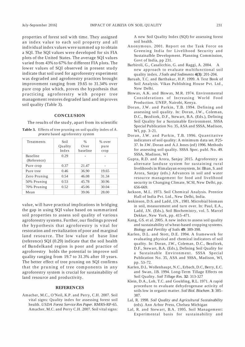
July-September 2016] IMPACT OF ALBIZIA ON SOIL QUALITY 231
properties of forest soil with time. They assignedan index value to each soil property and allindividual index values were summed up to obtaina SQI. The SQI values were developed for six FIAplots of the United States. The average SQI valuesvaried from 43% to 67% for different FIA plots. Thelower values of SQI observed in present studyindicate that soil used for agroforestry experimentwas degraded and agroforestry practices broughtimprovement ranging from 19.65 to 31.34% overpure crop plot which, proves the hypothesis thatpracticing agroforestry with proper treemanagement restores degraded land and improvessoil quality (Table 3).
CONCLUSION
The results of the study, apart from its scientific
A new Soil Quality Index (SQI) for assessing forestsoil health.
Anonymous. 2001. Report on the Task Force onGreening India for Livelihood Security andSustainalble Development. Planning Commission,Govt of India, pp 231.
Barbiroli, G., Casalicchio, G. and Raggi, A. 2004. Anew approach to evaluate multifunctional soilquality index. J Soils and Sediments 4(3): 201-204.
Baruah, T.C. and Barthakur, H.P. 1999. A Text Book ofSoil Analysis. Vikas Publishing House Pvt. Ltd.,New Delhi.
Biswas, A.K. and Biswas, M.R. 1974. EnvironmentalConsiderations of Increasing World FoodProduction. UNEP, Nairobi, Kenya.
Doran, J.W. and Parkin, T.B. 1994. Defining andassessing soil quality. In: Doran, J.W., Coleman,D.C., Bezdicek, D.F., Stewart, B.A. (Eds.), DefiningSoil Quality for a Sustainable Environment. SSSASpecial Publication No. 35, ASA and SSSA, Madison,WI, pp. 3–21.
Doran, J.W. and Parkin, T.B. 1996. Quantitativeindicators of soil quality: A minimum data set. P25-37. In J.W. Doran and A.J. Jones (ed) 1996. Methodsfor assessing soil quality. SSSA Spec. publ. No. 49.SSSA, Madison, WI
Gupta, R.D. and Arora, Sanjay 2015. Agroforestry asalternate landuse system for sustaining rurallivelihoods in Himalayan ecosystem, In: Bhan, S. andArora, Sanjay (eds.) Advances in soil and waterresource management for food and livelihoodsecurity in Changing Climate, SCSI, New Delhi, pp.656-669.
Jackson, M.L. 1973. Soil Chemical Analysis. PrenticeHall of India Pvt. Ltd., New Delhi, India.
Jenkinson, D.S. and Ladd, J.N., 1981. Microbial biomassin soil, measurement and turn over. In: Paul, E.A.,Ladd, J.N. (Eds.), Soil Biochemistry, vol. 5. MarcelDekker, New York, pp. 415–471.
Kang, GS. et al. 2005. A new index to assess soil qualityand sustainability of wheat-based cropping systems.Biology and Fertility of Soils 49: 389-398.
Karlen, D.L. and Stott, D.E. 1994. A framework forevaluating physical and chemical indicators of soilquality. In: Doran, J.W., Coleman, D.C., Bezdicek,D.F., Stewart, B.A. (Eds.), Defining Soil Quality fora Sustainable Environment. SSSA SpecialPublication No. 35, ASA and SSSA, Madison, WI,pp. 53–72.
Karlen, D.L. Wollenhaupt, N.C., Erbach, D.C, Berry, E.C.and Swan, J.B. 1994. Long-Term Tillage Effects onSoil Quality. Soil Tillage Res. 32: 313-327
Klein, D.A., Loh, T.C. and Goulding, R.L. 1971. A rapidprocedure to evaluate dehydrogenase activity ofsoils low in organic matter. Soil Biol. Biochem. 3: 385–387.
Lal, R. 1998. Soil Quality and Agricultural Sustainability(eds). Ann Arbor Press, Chelsea Michigan
Lal, R. and Stewart, B.A. 1995. Soil Management:Experimental basis for sustainability and
Table 3. Effects of tree pruning on soil quality index of A.procera based agroforestry system
Treatments Soil % % overQuality Over pureIndex baseline crop
Baseline 0.29 - - (Reference)Pure crop 0.37 21.47 -Pure tree 0.46 36.90 19.65Zero Pruning 0.54 46.08 31.3450% Pruning 0.53 45.78 30.9670% Pruning 0.52 45.06 30.04Mean 39.06 28.00
value, will have practical implications in bridgingthe gap in using SQI value based on summarizedsoil properties to assess soil quality of variousagroforestry systems. Further, our findings provedthe hypothesis that agroforestry is vital forrestoration and revitalization of poor and marginalland resource. The low value of base line(reference) SQI (0.29) indicate that the soil healthof Bundelkand region is poor and practice ofagroforestry holds the potential to improve soilquality ranging from 19.7 to 31.3% after 10 years.The better effect of tree pruning on SQI confirmsthat the pruning of tree components in anyagroforestry system is crucial for sustainability ofland resource and productivity.
REFERENCES
Amacher, M.C., O’Neil, K.P. and Perry, C.H. 2007. Soilvital signs: Quality index for assessing forest soilhealth. USDA Forest Service Res Paper. RMRS-RP-65.Amacher, M.C. and Perry C.H. 2007. Soil vital signs:

232 PRASAD et al. [Journal of Soil & Water Conservation 15(3)
environmental quality (eds). CRC/Lewis Publishers,Boca Raton, FL
Mohanty, M., Painuly, D.K., Mishra, A.K. and Ghosh,P.K. 2005. Soil quality effects of tillage and residueunder rice-wheat cropping on Vertisol in India.Commu.soil Sci. Plant Analysis 36(9):1162-1176.
Mukherjee, A. and Lal, R. 2014. Comparison of soilquality index using three methods. PLoS ONE. 9(8):e105981. doi:10.1371/journal.pone.0105981.
Nair, P.K.R. 1993. An Introduction to Agroforestry.Kluver, Boston
Oldeman, L.R. 1994.The Global Extent of SoilDegradation. In: D.J Greenland and I. Szabolcs(Eds.), Soil Resilience and Sustainable land, CAB,International, Wallingford, U.K. pp.99-118.
Olsen, S.R., Cole, C.V., Watanabe, F.S. and Dean, L.A.1954. Estimation of available phosphorus in soils byextraction with sodium bicarbonate. USDA Circular939, Washington.
Prasad Rajendra, Ram Newaj, N.K. Saroj V.D. Tripathiand S.K. Dhyani. 2015. Pattern of soil organic carbondecomposition in some agroforestry systems inBundelkhand Region of Central India. Indian Journalof Agroforestry 17(2): 18-21.
Prasad, Rajendra, Dhyani S.K., Ram Newaj, Kumar,Sudhir and Tripathi, V.D. 2016. Contribution ofadvanced agroforestry research in sustaining soilquality for increased food production and food security.Journal of Soil and Water Conservation 15(1): 31-39.
Ram Newaj, Dar S.A., Bhargava, M.K., Yadav, R.S. and
Ajit. 2007. Effect of Management practices on whitesiris (Albizia procera), grain yield of intercrops, weedpopulation and soil fertility changes inagrisilviculture system in semi-arid India. IndianJournal of Agric. Sci. 77(7): 17-20.
Roming, D.E., Garlynd, M.J, Harris, R.F. andMcSweeney, K. 1995. How farmers assess soil healthand quality. J. Soil Water Conserv. 50: 229-2236.
Sanchez, P.A. 1987. Soil productivity and sustainabilityin Agroforestry systems. In H.A. Seppler and P.K.R.Nair (Eds.), Agroforestry: A Decade ofDevelopment. International Council for Research inAgroforestry, Nairobi, Kenya, pp. 205-223.
Sharma, A. and Arora, Sanjay 2010. Soil quality indicesand relative production efficiency for maize andwheat crops in different agro-climates of North-WestIndia. Soil Science 175 (1): 44-49.
Solanki, R. and Arora, Sanjay 2015. Leaf litter dynamicsin agroforestry system affecting microbial activityin saline soils. Journal of Soil and Water Conservation14(4): 332-339.
Subbiah, B.V. and Asija, G.L. 1956. A rapid procedurefor assessment of available nitrogen in soils. Curr.Sci. 31:196–260.
Veihmeyer, F.J. and Hendrickson, A.H. 1948. Soildensity and root penetration. Soil Sci. 65: 487–493.
Walkley, A.J. and Black, C.A. 1934. An estimation of theDegtjareff method for determining soil organicmatter and a proposed modification of the chromicacid titration method. Soil Sci. 37: 29–38.

July-September 2016] COMPARATIVE STUDY OF REFERENCE ET 233
Journal of Soil and Water Conservation 15(3): 233-241, July-September 2016ISSN: 022-457X
Comparative study of reference evapotranspirationestimation methods including Artificial Neural Network for
dry sub-humid agro-ecological region
SASWAT KUMAR KAR1, A.K. NEMA1, ABHISHEK SINGH1, B.L. SINHA2 and C.D. MISHRA1
Received: 14 May 2016; Accepted: 6 August 2016
ABSTRACT
In the present study, an attempt has been made to compare the reference evapotranspiration (ETo),computed by eight different methods, namely, Penman-Monteith, Modified Penman-Monteith,Hargreaves-Samani, Irmak, Hargreaves, Valiantzas, ANN and FAO(24) model for the dry sub-humid agro-ecological region (Varanasi). An attempt was also made to find out utility of artificialneural networks (ANN) for estimation of ET0 with minimum input. Feed forward network hasbeen used for prediction of ETo using resilient back-propagation method and the architecture 2-2-1(having parameters Tmean and solar radiation) was found to be the best one. The average annualevapotranspiration (by Penman–Monteith method) for Varanasi was found to be 1447.4 mm. Whencompared among the different methods for estimation of reference evapotranspiration with Penman-Monteith method, the FAO-24 and Hargraves-Samani (3) under estimate, however, ModifiedPenman-Monteith, Hargreaves-Samani, Irmak, Hargreaves, Valiantzas over-estimate and ANNclosely estimates reference evapotranspiration.
Key words: Reference evapotranspiration, ANN, Trends, Penman-Monteith method
1 Institute of Agricultural Sciences, Banaras Hindu University, Varanasi-221005 (U.P.); 2College of Agricultural Engineering &Technology & Research (IJKVV) Mungali (C.G.); Email: anupamnema@ gmail.com
INTRODUCTION
Reference evapotranspiration (ETo) is animportant parameter of the hydrologic cycle andits accurate estimation is important for manystudies, such as hydrologic water balance,irrigation scheduling, water resources planning-management and for hydrologic and climaticstudies. Evapotranspiration (ET) is the combinedprocess of evaporation from the soil and plantsurfaces and transpiration through the stomata ofthe plant surface. The evapotranspiration rate froma reference surface having no shortage of water iscalled the reference crop evapotranspiration (ETo).The reference surface is a hypothetical grass withspecific characteristics. The concept of the referenceevapotranspiration was introduced to study theevaporative demand independent from crop type,crop development and management practices. Theonly factors affecting ETo are climatic parametersand can be computed from weather data. Manyequations are used to estimate ETo and can bedivided into two main groups, those that arephysically based like Penman, Penman-Monteith
model, etc. and those that are empirical based likeHargreaves, Hargreaves-Samani, Blaney-Criddlemodel, etc. but the comparison between the resultsof these methods reveals a wide divergence(Doorenbos and Pruitt, 1977). ETo expresses theevaporating power of the atmosphere at a specificlocation and time of the year and does not considerthe crop characteristics and soil factors. The FAOPenman Monteith method is the most reliablemethod for determining ETo as it explicitlyincorporates both physiological and aerodynamicparameters. It is a method with strong likelihoodof correctly predicting ETo in a wide range oflocations and climates and has provision forapplication even when some data is missing.Artificial neural network (ANN) technique hasdrawn the attention of many researchers becauseof the nature of being efficient and havingnonlinear modeling of complex systems. Manystudies have been done on the reliability of ANNsfor estimating ETo. Kisi (2007) compared thepotential of different ANN techniques andempirical methods in reference evapotranspiration

234 KAR et al. [Journal of Soil & Water Conservation 15(3)
estimation. In the present study, an attempt hasbeen made to estimate the referenceevapotranspiration by different known methodswith the objective to reduce the input weatherparameters (due to no availability of variousweather data) without losing the qualitative result.
MATERIALS AND METHODS
Study areaMeteorological data from the observatory of
Institute of Agricultural sciences, BHU, Varanasi(Latitude: 25.26 N, Longitude: 82.99E and Altitude:80.71 m) were collected and analysed for thepurpose of this study. The observatory is situatedin the dry sub humid agro ecological region (BHU,Varanasi). The meteorological data i.e. maximumtemperature (Tmax), minimum temperature (Tmin),maximum relative humidity (RHmax), minimumrelative humidity (RHmin), sunshine hour, windspeed, rainfall and pan evaporation of period of29 years (1986-2014) were used for present study.FAO has recommended the Penman-Monteithmethod for estimation of referenceevapotranspiration as it is a close, simplerepresentation of the physical and physiologicalfactors governing the evapotranspiration process.But, this method requires various meteorologicalparameters that are usually not available in mostmeteorological stations. Here, some other standardmethods like FAO-24 (Pan) model, Modified PMmethod, Hargreaves method, Hargreaves Samanimethod, Valiantzas method, Irmak method, ANN,etc are tested for estimation of ET0. ANN was alsotested and input parameters were optimized. Thedifferent methods of estimation of referenceevapotranspiration as mentioned above with therequired input parameters are discussed below.
FAO-56 (Penman Monteith) methodThe Penman Monteith method is considered as
standard because it has ranked first for both humidand arid regions (Allen et al., 1998). The equationthat is used for calculating the referenceevapotranspiration is given below:
(1)
where,
ETo = Reference evapotranspiration [mm day-1]Rn = Net radiation at the crop surface [MJm-2 day-1]G = Soil heat flux density [MJ m-2 day-1]
T = Mean of daily air temperature [°C]u2 = Wind speed at 2 m height [m s-1]es = Saturation vapour pressure [kPa]ea = Actual vapour pressure [kPa]∆ = Slope vapour pressure curve [kPa °C -1]λ = Psychrometric constant [kPa °C-1].
The parameters: air temperature, sunshineduration, wind speed and relative humidity aretaken directly from the meteorological station andare used to estimate other parameters such as thenet radiation, slope of saturation vapour pressurecurve, psychrometric constant, etc.
Modified Penman Monteith methodDue to difficulties in getting data, particularly
solar radiation, wind speed etc. Valiantzas (2006)suggested the simplified algebraic formula forPenman’s equation, which requires commonlyavailable data of mean temperature, solarradiation, mean relative humidity and wind speed.
(2)
where, T is the mean air temperature for theexamined time interval (0c), Q is the reflectioncoefficient or albedo with typical value of thealbedo for a grass cover is 0.23, Ra is theextraterrestrial radiation (MJm2d-1), RHmean is themean relative humidity for the examined timeinterval(%) and fu=au+(bu*U), where au =1, bu=0.54.
FAO-24 (Pan) modelEvaporation from pan (USWB Class A Land
Pan) is due to combined effect of temperature,relative humidity, wind speed, sunshine hour, etc.It is used in case of limited data condition. Thereference evapotranspiration as given by FAO(Pan) model is given by:
ETo = Epan * Kp (3)
where, ETo = Reference evapotranspiration,(mm day-1)
Epan = Pan evaporation, (mm day-1)Kp = Pan coefficient (0.7)
Hargreaves methodHargreaves (1975) suggested equation for
reference evapotranspiration based on solarradiation, maximum temperature and minimumtemperature as follows:
(4)
July-September 2016] COMPARATIVE STUDY OF REFERENCE ET 235
Hargreaves Samani methodThe extraterrestrial radiation based equation of
Hargreaves and Samani (1985) requiring only thedata for Ra, Tmax and Tmin is as follows:
(5)
Valiantzas methodA simplified form of modified PM equation
requiring only solar radiation (Rs), Tmean-, RHmeantakes the following form (Valiantzas, 2013).
(6)
Irmak methodIrmak et al. (2003) developed following
simplified equation for estimation of ETo usingsolar radiation and mean temperature.
(7)
Artificial Neural NetworkArtificial Neural Network (ANN) offers a
relatively quick and flexible means of modelling.It gives complex nonlinear relationship among thedependent and independent variables, due towhich it has received enormous interest byresearcher and widely used for calculation ofevaporation under limited weather data. An ANNis a computer model, composed of individualprocessing elements called units or neurons andthey are highly interconnected and operate inparallel, these elements are inspired by biologicalnervous systems. In this study, the neural networksare adjusted or trained with a series of inputs sothat a particular input leads to a specific targetoutput from the training data set. In the ANNanalysis MLP type of feed-forward neural networkwith back propagation learning algorithm isapplied with input layer, hidden layer and outputlayer. Basically, it is a gradient descent techniqueto minimize the squared error between thecalculated and predicted outputs. In this study,since the purpose of this study was the estimationof ETo, the ANN has only one output variable. Theoutput of a neuron is decided by an activationfunction. There are a number of activationfunctions that can be used in ANNs, such as step,sigmoid, threshold, linear, etc. The sigmoidactivation function [f(x)] commonly used, can beformulated mathematically as:
The database was divided into three subsets:65% of data are used in the training phase, 20% inthe testing phase; 15% for validation. The first setis for determining the weights and biases of thenetwork, the second one is for evaluating theweights and biases and to decide when to stoptraining and the last data set is for validating theweights and biases to verify the effectiveness ofthe stopping criterion and to estimate the expectednetwork operation on new data sets. The ideabehind this division is to overcome the over fittingproblem. The PM estimated daily ET0 values wereemployed as substitute for measured ET0 data andused as target output. Results showed thatincreasing the number of neurons in hidden layerdid not improve the ANN results as reported byKisi (2006), but too many neurons may lead to theover fitting. So the number of hidden nodes in theANN architecture was identified by trial and error(Moghaddamnia et al., 2009). These computed ET0values were used to train the ANN models. Variousarchitectures and input combinations of the modelswere compared for crop evapotranspiration. Theinput variables considered in the input layerdecrease gradually according to their reducedsensitivity i.e. Tmean>VPD >RS > U2as suggestedby Anupriya et al. (2014) by calculating a sensitivitycoefficient of ETo to each climate variable (Irmaket al., 2006). Input parameters decrease from fourto one and their effect on predicted ETo is analyzed.
Accuracy criteriaAccuracy tests were performed to evaluate the
reference evapotranspiration estimated by differentmethods by the statistical analysis, as shown intable in next page.
RESULTS AND DISCUSSION
Food and Agriculture Organization (FAO) hassuggested that the Penman-Monteith method is thestandard method for estimation of potentialevapotranspiration. The average annualevapotranspiration for Varanasi is found tobe 1447.4 mm and the average dailyevapotranspiration is found to be 3.96 mm/day bythe above method. The daily average referenceevapotranspiration varies from minimum 1.65mm/day to maximum 6.77 mm/day. Anupriya etal. (2014) has suggested that Tmean, Vapour PressureDeficit (VPD), solar radiation (RS) and wind speed(U2) are the parameters which are most sensitivein the decreasing order towards referenceevapotranspiration. Artificial Neural Networktechnique was utilised with the different

236 KAR et al. [Journal of Soil & Water Conservation 15(3)
combination of these four sensitive parametersas input for estimation of referenceevapotranspiration. To find out the best ANNarchitecture, providing near accurate estimationof evapotranspiration with limited climatic data,first of all the optimum number of nodes in hiddenlayer for each ANN architecture were decided byrunning the ANN analysis to a number of timesuntil a significantly least relative error is found inthe holdout. The best ANN architecture was chosenand evaluated among various ANN architectureswith different number of neurons in hidden layer.Table 1, represent the results obtained from ANNof feed forward with learning algorithm of backpropagation (BP) type. For statistical comparisonof performance of these ANN architectures, the
predicted evapotranspiration by these neuralnetworks were compared with the estimatesprovided by the FAO-56(PM) evaporation model.The detail performance evaluation is briefed in theTable 1.
The ANN architecture 4-3-1 estimatedevapotranspiration with maximum accuracy, i.e.relative error (Holdout) = 0.001, MSE = 0.003 mmday-1, RMSE = 0.053 mm day-1, r = 0.992 and r2 =0.985. But, this architecture requires four inputparameters. While the ANN architecture 2-2-1requires only two input parameters i.e., Tmean, solarradiation (Rs) and estimate evapotranspirationquite accurately with less error i.e., relative error(Holdout)= 0.005, MSE =0.017 mm day-1, RMSE =0.130 mm day-1, r = 0.988 and r2= 0.976. Therefore,
Performance Criteria Formula RemarksMean Square Error An MSE of zero, means that the ‘Pi’ predicts(MSE) observation of the parameter ‘Ei’ with perfect
accuracy.
Root Mean square error Flemming (1975)(RMSE)Coefficient of It always lies between -1 to +1, if r =1, thecorrelation (r) correlation coefficient is perfect and positive
and if r = -1, then it is perfect and negative.Coefficient of Coefficient of determination (r2) is a statisticaldetermination (r2) measure of how well the regression line
approximates the real data points. An r2 of 1indicates that the line of regression is of best fit.
where, Pi = Predicted ETo, Ei = Estimated ETo, N = Number of observation
Table 1. Comparison of various neural network predicted ETo data with FAO-56 (PM) estimated ETo
ANN architecture 4-3-1 3-3-1 2-2-1 1-9-1 3-5-1 2-6-1 2-3-1Inputs Tmean, Tmean, Tmean, Tmean Solar Tmean, Solar
Solar Solar Solar radiation U2 radiation radiation, radiation radiation (Rs), (Rs), VPDVPD, U2 (Rs), VPD (Rs) ( VPD, U2)
No of neuronsInput 4 3 2 1 3 2 2Hidden 1 1 1 1 1 1 1Output 1 1 1 1 1 1 1Nodes in hidden layer 3 3 2 9 5 6 3MSE 0.003 0.015 0.017 0.624 0.024 0.129 0.185RMSE 0.053 0.124 0.130 0.790 0.156 0.359 0.430Coefficient of 0.992 0.989 0.988 0.920 0.985 0.959 0.944correlation (r)Coefficient of 0.985 0.978 0.976 0.846 0.970 0.920 0.892determination (r2)Relative Error 0.001 0.006 0.005 0.089 0.009 0.034 0.061(Holdout)
where, Tmean= Daily mean temperature (°C), Solar radiation (Rs) on daily basis, Vapour Pressure Deficit (VPD) = es-ea,U2= Wind speed daily basis
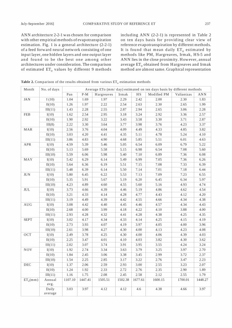
July-September 2016] COMPARATIVE STUDY OF REFERENCE ET 237
ANN architecture 2-2-1 was chosen for comparisonwith other empirical methods of evapotranspirationestimation. Fig. 1 is a general architecture (2-2-1)of a feed forward neural network consisting of oneinput layer, one hidden layers and one output layerand found to be the best one among otherarchitectures under consideration. The comparisonof estimated ETo values by different 9 methods
including ANN (2-2-1) is represented in Table 2on ten days basis for providing clear view ofreference evapotranspiration by different methods.It is found that mean daily ETo estimated bymethods like PM, Hargreaves, Irmak, HS-5 andANN lies in the close proximity. However, annualaverage ETo obtained from Hargreaves and Irmakmethod are almost same. Graphical representation
Table 2. Comparison of the results obtained from various ETo estimation methods
Month No. of days Average ETo (mm/day) estimated on ten days basis by different methodsPan P-M Hargreaves Irmak HS Modified PM Valiantzas ANN
JAN I (10) 1.04 1.69 1.97 2.29 2.42 2.00 2.30 1.83II(10) 1.26 1.97 2.22 2.54 2.63 2.30 2.65 1.99III(11) 1.43 2.28 2.55 2.87 2.94 2.65 3.06 2.28
FEB I(10) 1.62 2.54 2.95 3.18 3.24 2.92 3.36 2.57II(10) 1.90 2.92 3.22 3.43 3.58 3.30 3.71 2.87III(8) 2.22 3.30 3.64 3.77 3.98 3.76 4.23 3.37
MAR I(10) 2.56 3.76 4.04 4.09 4.49 4.33 4.85 3.82II(10) 3.03 4.20 4.41 4.35 5.11 4.78 5.24 4.10III(11) 3.86 4.83 4.90 4.68 5.85 5.51 6.01 4.63
APR I(10) 4.59 5.39 5.46 5.05 6.54 6.09 6.79 5.22II(10) 5.13 5.69 5.58 5.15 6.98 6.54 7.08 5.60III(10) 5.59 6.06 5.98 5.40 7.10 6.89 7.36 6.08
MAY I(10) 5.42 6.29 6.14 5.49 6.99 7.05 7.36 6.26II(10) 5.64 6.36 6.19 5.51 7.15 7.08 7.33 6.39III(11) 5.48 6.39 6.14 5.50 7.14 7.01 7.18 6.44
JUN I(10) 5.80 6.45 6.22 5.53 7.13 7.09 7.23 6.55II(10) 5.35 5.91 5.67 5.19 6.20 6.45 6.34 5.97III(10) 4.23 4.89 4.60 4.55 5.60 5.16 4.93 4.74
JUL I(10) 3.73 4.66 4.39 4.46 5.19 4.86 4.62 4.54II(10) 3.21 4.33 4.14 4.28 4.77 4.43 4.12 4.20III(11) 3.19 4.49 4.39 4.42 4.55 4.66 4.34 4.38
AUG I(10) 3.08 4.42 4.40 4.45 4.46 4.57 4.34 4.43II(10) 2.68 4.00 3.99 4.18 4.22 4.10 3.88 4.00III(11) 2.93 4.28 4.32 4.41 4.28 4.38 4.25 4.35
SEPT I(10) 3.02 4.17 4.34 4.33 4.14 4.25 4.15 4.19II(10) 2.73 3.93 4.07 4.19 3.97 4.05 4.00 3.96III(10) 2.61 3.98 4.27 4.30 4.00 4.13 4.23 4.08
OCT I(10) 2.49 3.78 4.25 4.30 4.00 4.06 4.39 4.03II(10) 2.25 3.47 4.01 4.10 4.03 3.82 4.30 3.62III(11) 2.02 3.07 3.74 3.91 3.95 3.55 4.24 3.24
NOV I(10) 1.92 2.74 3.34 3.63 3.79 3.25 3.97 2.70II(10) 1.84 2.45 3.06 3.38 3.45 2.99 3.72 2.37III(10) 1.54 2.25 2.85 3.17 3.22 2.76 3.47 2.23
DEC I(10) 1.37 2.06 2.59 2.93 3.00 2.55 3.23 2.07II(10) 1.24 1.92 2.33 2.72 2.76 2.35 2.90 1.89III(11) 1.16 1.75 2.08 2.45 2.58 2.12 2.55 1.79
ETo(mm) Annual 1107.10 1447.41 1505.51 1502.38 1677.61 1600.15 1700.01 1448.27avg.
Daily 3.03 3.97 4.12 4.12 4.6 4.38 4.66 3.97average

238 KAR et al. [Journal of Soil & Water Conservation 15(3)
of average ETo by different methods on monthlybasis is shown in Fig 2. It shows maximum EToduring month of May and lowest during monthof Dec-Jan. When compared among thedifferent methods for estimation of referenceevapotranspiration with standard Penman-Monteith method, it is found that Pan (FAO-24)under estimate and Modified Penman-Monteith,Hargreaves-Samani, Irmak, Hargreaves, Valiantzasoverestimate however ANN closely estimatesreference evapotranspiration.
Long term changes in evaporation and potentialevapotranspiration can have profoundimplications for hydrological process as well as foragricultural crop performance. Large changes inthe evapotranspiration demand would change thewater requirement and water balance in the cropgrowing seasons. Trend analysis as shown in Fig.3 depicts the decreasing trend. It has also observedthat annual reference crop evapotranspiration
varies from 1553.02 mm (year 1993) to 1383.58 mm(year 2013). Similar trends were also observed byRao and Wani (2011) for semi-arid climate ofICRISAT, Hyderabad.
Pan evaporation data is available at almost allmetrological observatories. An attempt was madeto correlate these Pan data with other estimationmethods. The results of statistical analysis (Table3) shows that Penman- Monteith method have aclose relationship with Pan method having MSE=0.968, RMSE= 0.984 and coefficient of correlation(r) = 0.977 followed by ANN having MSE= 1.002,RMSE= 1.001 and coefficient of correlation (r) =0.971. Similar pattern was also found by Kale et al.(2013). A single linear regression (y = mx + c) foreach estimation was also accomplished by plottingthe scatter plot for the test data with respect to dataobtained from FAO-24 estimations and is depictedin Fig. 4 to 10.
Table 3. Statistical comparison of ETo estimated by different methods with ETo estimated by FAO-24 (Pan) model
ETo estimation MSE RMSE Coefficient of Coefficient of Conversion Equation from Cmethods correlation (r) determination (r2) Pan model to others (y intercept)Penman- 0.968 0.984 0.977 0.955 Y1 = 0.9591X + 1.056 1.056MonteithHargreaves 1.397 1.182 0.960 0.922 Y2 = 0.8051X + 1.683 1.683Irmak 1.649 1.284 0.940 0.884 Y3 = 0.5877 X + 2.334 2.334Hargreaves- 2.534 1.592 0.979 0.959 Y4 = 0.973 X + 1.645 1.645SamaniMod PM 1.899 1.378 0.985 0.970 Y5 = 1.0309 X + 1.257 1.257Valiantzas 2.852 1.689 0.952 0.907 Y6 = 0.9663 X + 1.727 1.727ANN 1.002 1.001 0.971 0.942 Y7 = 0.9457 X + 1.100 1.100
where, X = Estimated ETo by Pan method and Y1, Y2, Y3, Y4, Y5, Y6 and Y7 are estimated ETo by Penman- Monteith, Hargreaves,Irmak, Hargreaves samani, Modified PM, Valiantzas and ANN methods, respectively.
Fig. 1. Architecture (2-2-1) of feed forward neural network with one hidden layer

July-September 2016] COMPARATIVE STUDY OF REFERENCE ET 239
Fig. 2. Monthly average reference evapotranspiration (ETo) by different 8 methods
Fig. 3. Trend in reference crop evapotranspiration (ETo) at Varanasi, UP
Fig. 4. Reference evapotranspiration by Pan Vs P-M
Fig. 5. Reference evapotranspiration by Pan Vs Hargreaves method

240 KAR et al. [Journal of Soil & Water Conservation 15(3)
Fig. 6. Reference evapotranspiration by PAN Vs IRMAK
Fig. 8. Reference evapotranspiration by Pan Vs Modified PM
Fig.9. Reference evapotranspiration by Pan Vs Valiantzas
Fig. 10. Reference evapotranspiration by Pan Vs ANN
Fig. 7. Reference evapotranspiration by Pan Vs Hargreaves-Samani

July-September 2016] COMPARATIVE STUDY OF REFERENCE ET 241
CONCLUSION
Estimation of the crop evapotranspiration isvery useful for crop planning in dry Sub-humidAgro-ecological region. In case of limited weatherdata, Artificial Neural Network (architecture: 2-2-1) with input parameters mean temperature andsolar radiation (Rs) estimate the referenceevapotranspiration very accurately. The Pan datacan be correlated with penman Monteith methodhigh degree of correlation.
REFERENCES
Allen, R.G., Pereira, L.S., Raes, D. and Smith, M. 1998.Crop evapotranspiration- Guidelines for computingcrop water requirements. Journal of irrigation anddrainage engineering. Paper No. 56, FAO, Rome.
Doorenbos, J. and Pruitt, W. O. 1977. Guidelines forcomputing crop water requirements. (FAO). Journalof irrigation and drainage engineering. Paper No.24 (rev). FAO, Rome.
Hargreaves, G. H. and Samani, Z. A. 1985. Referencecrop evapotranspiration from temperature. AppliedEngineering in Agriculture 1(2): 96-99.
Hargreaves, G. H. 1975. Moisture availability and cropproduction. Trans. American Society of AgriculturalEngineering 18(5): 980-984.
Irmak, S., Payero, J. O., Martin, D. L., Irmak, A. andHowell, T. A. 2006. Sensitivity analyses andsensitivity coefficients of standardized daily ASCEPenman-Monteith equation. Journal of Irrigation andDrainage Engineering 132(6): 564-578.
Irmak, S., Allen, R. G. and Whitty, E. B. 2003. Daily grass
and Alfalfa- reference evapotranspiration estimatesand Alfalfa to grass evapotranspiration ratios inFlorida. Journal of Irrigation and Drainage Engineering129(5): 360-370.
Kale, M. U., Nagdeve, M. B. and Bagade, S. J. 2013.Estimation of evapotranspiration with ANNtechnique. Journal of Indian Water Resources Society33(1): 23-29.
Kisi, O. 2006. Daily pan evaporation modelling using aneuro-fuzzy computing technique. J. Hydrol .(Amsterdam). 329: 636–646.
Kisi, O. 2007. Evapotranspiration modeling fromclimatic data using a neural computing technique.Hydrol. Processes 21(14): 1925-1934.
Moghaddamnia, A., Ghafari Gousheh, M., Piri, J., Amin,S. and Han, D. 2009. Evaporation estimation usingartificial neural networks and adaptive neuro-fuzzyinference system techniques. Adv. Water Resource32(1): 88-97.
Priya, A., Nema, A. K. and Islam, Adlul 2014. Effect ofclimate change and elevated CO2 on referenceevapotranspiration in Varanasi, India - A case study.Journal of Agrometeorology 16(1): 1-8.
Rao, A. and Wani, S. 2011. Evapotranspiration paradoxat a semi-arid location in India. Journal ofAgrometeorology 13(1): 3-8.
Valiantzas, J. D. 2006. Simplified versions for thePenman evaporation equation using routineweather data. J. Hydrol. 331(3-4): 690-702.
Valiantzas, J. D. 2013. Simple ETo forms of Penman’sequation without wind and/or humidity data. I:Theoretical development. Journal of Irrigation andDrainage Engineering 139(1): 1-8.
242 ADHIKARI et al. [Journal of Soil & Water Conservation 15(3)
Journal of Soil and Water Conservation 15(3): 242-245, July-September 2016ISSN: 022-457X
Efficient use of jute agro textiles as soil conditioner toincrease chilli productivity on Inceptisol of West Bengal
NABANITA ADHIKARI, ARIF DISHA, ANGIRA PRASAD MAHATA, ARUNABHA PAL,RAHUL ADHIKARI, MILAN SARDAR, ANANYA SAHA, SANJIB KUMAR BAURI,
P. K. TARAFDAR and SUSANTA KUMAR DE
Received: 22 July 2016; Accepted: 13 September 2016
ABSTRACT
A field experiment was conducted at the University farm of Regional Research Station, New Alluvialzone of Bidhan Chandra Krishi Viswavidyalaya, Gayespur under Nadia district of West Bengalwhich is situated at 220 58’ 31’’ N L, 880 26’ 20’’ E L, with an altitude at 10.9 m above the mean sealevel to investigate the effect of various strength (gram per meter square) of jute agro textiles onchange of soil properties on chilli yield. Five treatment combinations viz. T1 - farmers practices(control), T2 - 200 GSM jute agro textiles, T3- 400 GSM jute agro textiles, T4 - 600 GSM jute agrotextiles and T5- 800 GSM jute agro textiles were spread before transplanting of chilli seedlingsalong with the levels of N-P-K at 50-25-25 kg/ ha and in RBD design with four réplications. Initialsand final soil samples were analyzed for relevant physical and chemical properties by followingstandard methods. The yields of crop were found 10.00, 16.26, 17.57, 14.02 and 12.00t/ha respectivelyin T1, T2, T3. T4 and T5. The yield of crop was increased 7.57t/ha (75.7%) under 400 GSM jute agrotextiles over – farmers practices (control). The result showed the decreased bulk density and increasedporosity under all treatments. They also improved moisture use efficiency, in general, by 96.5%over control. Decreasing bulk density with simultaneous increasing of porosity under jute agrotextile treatments also improved the moisture retention capacity in soil. Better aggregation andtheir stabilization as well as chilli yield occurred with applied T3 - 400 GSM jute agro textilestreatments.
Key words: Jute agro textiles, bulk density, porosity and moisture use efficiency.
Department of Soil and Water Conservation, Bidhan Chandra Krishi Viswavidyalaya, Nadia, Mohanpur, West Bengal;Email: [email protected]
INTRODUCTION
Jute agro geo-textiles as surface cover materialshave various potentials for maintaining soil qualityand protecting the soil against any form ofdegradation. Naturally occurring jute agro geo-textiles are eco-friendly and biodegradableproducts which act as surface cover materials anduseful ameliorative to eliminate soil relatedconstraints to crop production (Yong et al., 2000;Pain et al., 2013). It also helps to protect the mostvital natural resources against various degradationprocesses and promotes vegetative cover throughaccelerated seed germination and seedlingemergence (Bhattacharya et al., 2010). Adequateinformation on the efficiencies of jute agro textilesas soil conditioners towards improving cropproductivity are lacking.
Chilli is an important cash crop in India and isgrown for its pungent fruits, which are used bothas green and ripe. Green chillies are rich in VitaminA and C, minerals and protein. Dry chillies are alsorich in Vitamin A and D. It is an essential item foralmost every Indian dishes and also used as sauces,chutneys and pickles and medicinal purposes.India as the largest producer of chillies in the world.Its production level covers around 1.1 million tonsannually. The major cultivated regions of chilli inIndia are AP, Karnataka, Maharashtra, UP, Punjab,TN, Rajasthan, Orissa, West Bengal and M.P. ofwhich Andhra Pradesh alone commands about46% of the production. However, the productivityof the crop gradually decreases due to decliningsoil fertility status and inadequate availabilities ofwater as well as non-availability of good qualityseeds.

July-September 2016] EFFICIENT USE OF JUTE AGRO TEXTILES 243
Keeping in view the above considerations, thepresent study was undertaken to compare theefficiencies of different strength (gram per metersquare) of jute agro textiles on soil quality changesand improvement of chilli yield in sub-tropicalcondition.
MATERIALS AND METHODS
The present investigation have been carried outat the university farm of Regional Research Station,New Alluvial Zone, Bidhan Chandra KrishiViswavidyalaya, Gayeshpur, Nadia District, WestBengal represented by sub-tropical climatic regionis situated at 220 58’ 31’’ N L, 880 26’ 20’’ E L, withan altitude at 10.9 m above the mean sea levelhaving average rainfall of 1500 to 1600 mm/yearwith variation of temperatures between 100 to 380
C. The soils of the area are characterized by acidicin nature, low in organic carbon and medium infertility status. The experiment was conducted withthe treatments: T1 : farmer’s practice (control), NPK@ 50-25-25 kg/ha; T2 : 200 GSM jute agro textiles +NPK @ 50-25-25 kg/ha; T3 : 400 GSM jute agrotextiles + NPK @ 50-25-25 kg/ha; T4 : 600 GSM juteagro textiles + NPK @ 50-25-25 kg/ha; T5: 800 GSMjute agro textiles + NPK @ 50-25-25 kg/ha whereGSM = gram per meter square.
All the treatments were replicated four times inRBD design with growing chilli (Capsicum annuum)(var. - Kajli bullet) as test crop. It was shown on 1st
week of February consecutively for the years of2015 and 2016. The area of each plots weremaintained by 20 sq.m with spacing of 75 cmbetween row to row and 75 cm between plants toplants. The recommended packages of practiceswere adopted for growing of the crop. Each yeargreen chilli crops were harvested started from 1st
week of April upto June. Jute agro textiles werelaid during the transplanting of chilli seedlings(Fig. 1). Bulk density and porosity of soil and soilmoisture contents of surface layer at 7 days interval
from entire growth period were determined bygravimetric method by Black (1965). The sizedistribution of aggregates in soil was evaluated bythe methods as proposed by Piper (1966). The pH,organic carbon, availabilities of phosphorous andpotassium were determined by the standardprocedure of Jackson (1965). Cost benefit ratios wascalculated by the ratio of total economic return (Rs)and total cost (Rs). Moisture use efficiency wascalculated by the relationship as: MUE (kg/mm/ha) = Total yield (kg/ha)/Consumptive use ofwater (mm). Necessary stastical analysis wasworked out to interpret the effects of treatmentsas suggested by Gomez and Gomez (1984).
RESULTS AND DISCUSSION
Chilli yieldThe results of effects of different strength of jute
agro textiles on yields of chilli presented in Table1 and (Fig. 2). Response of green chilli yield overcontrol due to treatments were 6.26 ton/ha (62.5%),7.57 ton/ha (75.7%), 4.02 ton/ha (40.2%) and 2.00ton/ha (20.00%) and dry chilli yield were 1.38 ton/ha (61.61%), 1.74 ton/ha (77.68%), 0.91 ton/ha(40.63%) and 0.41 ton/ha (18.30%), respectively in200 GSM jute agro textiles, 400 GSM jute agro
Table 1. Effect of different strength of jute agro textiles on chilli yield, MUE and BC ratio
Treatments Green Yield Dry Yield Moisture use Benefit(ton/ha) (ton/ha) efficiency Cost ratio
(kg/ha/mm) (B:C)( T1) Control (farmers practices) 10.00 2.24 35.6 1.2:1(T2 ) 200 GSM jute agro textiles 16.26 3.62 60.0 2.2:1(T3) 400 GSM jute agro textiles 17.57 3.98 67.5 2.4:1(T4)600 GSM jute agro textiles 14.02 3.15 66.3 2.1:1(T5) 800 GSM jute agro textiles 12.00 2.65 64.61 2.0:1SE(m)+ 0.16 0.03 0.01CD(0.05) 0.50 0.10 0.03
Fig 1. Two month aged chilli crop with jute agro textiles

244 ADHIKARI et al. [Journal of Soil & Water Conservation 15(3)
textiles, 600 GSM jute agro textiles and 800 GSMjute agro textiles. The significantly highest (P<0.05)green and dry chilli yield crop were observed in400 GSM jute agro textiles. The benefit cost ratioof chilli crop also maximum on 400 GSM jute agrotextiles. The results revealed that the maximumchilli yield under 400 GSM jute agro textilesprobably due to proper root growth towardsuninterrupted availability of nutrients throughcontinuous supply of moisture and air. The aboveresults find supported by Paza (2007).
Physical and chemical properties of soilThe results of the effects of different strength of
jute agro textiles on the changes of physical andchemical properties of soil are presented in Table2. Bulk density of soil were decreased by0.07(5.15%), 0.08(5.88%), 0.1(7.35%) and 0.13(9.56%)with simultaneous increased of porosity by6.9(17.00%), 9.0(22.17%), 8.2(20.20%) and6.1(15.02%) respectively in 200 GSM jute agrotextiles, 400 GSM jute agro textiles, 600 GSM juteagro textiles and 800 GSM jute agro textiles overcontrol. The results further indicated thatsignificantly increased availability of nitrogen,
phosphorous and potassium. The results alsoreveal the increment of organic carbon by0.09(13.64%), 0.23(34.85%), 0.31(46.97%) and0.38(57.58%) respectively in 200 GSM jute agrotextiles, 400 GSM jute agro textiles, 600 GSM juteagro textiles and 800 GSM jute agro textiles. Theresults revealed that the maximum porosity wasfound in 400 GSM jute agro textiles to increaseaeration and root growth towards uninterruptedavailability of nutrients. The above results are inagreement with those reported by Dutta andChakraborty (1995).
Soil moisture use efficiencySoil moisture changes at 7 days interval for the
entire growing period of chilli under variousstrength of jute agro textiles have been depicted inFig. 3. Soil moisture content at every stage washigher under each of the treatment over control. Itwas found maximum under 400 GSM jute geotextiles than other treatments. Results followed thefollowing order of soil moisture contents: 400 GSMjute geo textiles > 600 GSM jute geo textiles > 800GSM jute geo textiles > 200 GSM jute geo textiles >control. The changes of soil moisture content dueto the treatment might be attributed by bulk
Fig. 2. Three month aged chilli crop with fruits
Table 2. Effect of different strength of jute agro textiles on soil physical and chemical properties
Treatments Bulk Porosity pH Organic Total Available AvailableDensity (%) (1:2) Carbon N (%) P K
(Mg/m3) (%) (kg/ha) (kg/ha)( T1) Control (farmers practices) 1.36 40.6 6.2 0.66 0.09 16.7 145(T2 ) 200 GSM jute agro textiles 1.29 47.5 6.4 0.75 0.18 26.9 292(T3) 400 GSM jute agro textiles 1.28 49.6 6.5 0.89 0.22 27.9 306(T4)600 GSM jute agro textiles 1.26 48.8 6.6 0.97 0.28 29.7 320(T5) 800 GSM jute agro textiles 1.23 46.7 6.7 1.04 0.31 30.8 332SE(m)+ 0.005 0.389 0.01 0.02 0.04 0.30 0.20CD(0.05) 0.017 1.346 0.03 0.07 0.13 0.94 0.63
Fig. 3. Effect of various jute agro textiles management onchanges of soil moisture percent

July-September 2016] EFFICIENT USE OF JUTE AGRO TEXTILES 245
density and porosity in soil towards increasingmoisture retention capacity of soil. The data furthershowed that the moisture use efficiencies of thecrop, generally, increased by 81.47 % due to thetreatments of jute agro textiles over control, thehighest of 89.61 % which occurred under 400 GSMjute agro textiles (Table 1). The above resultssupported by Nag et al. (2008).
Soil aggregationThe results of the effects of jute agro textiles on
the changes of various indices of soil structure andtheir stabilization were presented in table 3. Resultsclearly revealed much variation of all the indicesof soil structure and their stability due toapplication of various treatments. The values ofmean weight diameter (MWD), geometric meandiameter (GMD), structural coefficient (SC) andwater stable aggregates (WSA) were found highestunder 400 GSM jute agro textiles followed by 600GSM jute agro textiles, 800 Gsm jute agro textiles,and 200 GSM jute agro textiles. These indicated that400 GSM jute agro textiles could be effectiveamelioration towards improving stability of soilstructure. The above results are supported by thefindings of Panchal et al. (2002).
CONCLUSION
Efficiencies of different strength of jute agrogeotextiles on the improvements of soil propertiesattributing yield of chilli have been investigatedin the present study. Sharp improvements of bulkdensity, porosity, moisture use efficiency as wellas better aggregation and well stabilization of soilaggregates occurred due to application of eachstrength of jute agro geotextiles in general, of which400 GSM jute agro textiles showed most prominenteffects on porosity and yield of chilli and benefit/cost ratio as well. The result thus leads to suggest
Table 3. Effect of different strength of jute agro textiles on soil structure and their stabilization
Treatments Mean Weight Structure Geometric Mean WSA>0.25 WSA<0.25Diameter (mm) Coefficient Diameter (mm) (%) (%)
( T1) Control (farmers practices) 1.21 0.91 0.78 58.97 41.03(T2 ) 200 GSM jute agro textiles 1.24 1.10 0.86 72.23 27.77(T3) 400 GSM jute agro textiles 2.95 1.27 1.41 84.74 15.51(T4)600 GSM jute agro textiles 2.37 1.23 1.21 82.88 17.12(T5) 800 GSM jute agro textiles 2.26 1.17 1.01 79.30 20.70SE(m)+ 0.01 0.11 0.01 0.99 0.99CD(0.05) 0.03 0.35 0.04 3.43 3.43
that 400 GSM jute agro textiles could be effectivelyutilized for chilli cultivation as its beneficial effectstowards favourable soil structure along with othersoil properties and uninterrupted availability ofwater, nutrient and air influencing root growthwhich in turn improves crop production.
REFERENCES
Bhattacharyya, R., Davies, K., Fullen, M. A. and Booth,C. A. 2010. Soil conservation using palm-matgeotextiles on loamy sand soils in the UnitedKingdom.
Black, C. A. 1965. Method of soil analysis. American Soc.Agron., Inc., Madison, Wisconsin, USA
Dutta, T. and Chakraborty, T. 1995. Effect of organicmanures and subabul leaf mulching under varyinglevels of fertility on growth and yield of potato andweed biomass. Indian Journal of Agron. 40(1): 140-142.
Gomez, K. A. and Gomez, A. A. 1984. StatisticalProcedures for Agricultural Research, 2nd Ed. Wiley,New York.
Jackson, M. L. 1967. Soil chemical analysis. Prentice Hallof India Pvt.Ltd., New Delhi, India.
Nag, D., Choudhury, T. K., Debnath, S., Ganguli, P. K.and Ghosh, S. K. 2008. Efficient management of soilmoisture with jute non-woven as mulch forcultivation of sweet lime and turmeric in red lateriticzone. Journal of Agri. Engg. 45(3): 59-62.
Pain, Debabrata, De, Susanta Kumar, Tarafdar, P. K.,Pal, Arunabha, Mahata, Angira Prasad, Adhikari,R. and Bauri, S.K. 2013. Efficient use of geotextilesas soil conditioner to increase potato productivityon inceptisols of West Bengal. Journal of Soil andConservation 12(2):103-107.
Paza, A. 2007. The fertilization of potato with cash cropsand straw. Framenta Agronomical 24(40): 100-105.
Piper, C S. 1966. Soil plant analysis. Asian Report, Hans,Puplisher, Bombay, India.
Yong, L. H., ZaiQin, W., DingXing, P. and GuoSheng,L. 2000. Study on the effect of jute geotextile on rimegrowth. Journal of Scientia Agricultura Sinica 33(3):103-105.

246 PANWAR and KUMAR [Journal of Soil & Water Conservation 15(3)
Journal of Soil and Water Conservation 15(3): 246-251, July-September 2016ISSN: 022-457X
Artificial Neural Network models for disaggregationof monsoon season runoff series for a hilly watershed
RAJDEV PANWAR and DEVENDRA KUMAR
Received: 25 April 2016; Accepted: 18 July 2016
ABSTRACT
This paper presents the application of artificial neural networks for disaggregating of monsoonseason comprising of June, July, August and September (JJAS) months of the year runoff series andis illustrated by an application to model the river flow of Naula watershed of Ramganga river inUttrakhand state, India. Two different seasonal ANN models were developed. In the first ANNmodel neural network was trained with monsoon season comprising of June, July August andSeptember (JJAS) months of the year runoff as input and runoff (corresponding to 4 months, JJAS)of June, July, August and September month output. The ANN architecture 1-1-1-4 was found bestin training and testing. In the second ANN model most active monsoon months (July and August)total runoff and relatively less active months (June and September) total runoff was used as inputand runoff of July and August; June and September runoff, respectively as output. The ANNarchitecture 1-4-4-4-2 for June-September total and 1-4-4-2 for July-August total was found best intraining and testing. Lower value of RMSE and higher value of CE was obtained for all the monthsfor the selected architecture. The correlation coefficient between measured and simulated data seriesare 0.92 and 0.75 for training and testing, respectively for model 1 whereas for model 2, the valuesare 0.99 and 0.87 in July-August and 0.97 and 0.89 in June-September for training and testing,respectively.
Key words: Disaggregation, Neural network, Levenberg-Marquardt algorithm
Department of Soil and Water Conservation Engineering, College of Technology, G.B. Pant University of Agriculture andTechnology, Pantnagar-263145, Uttarakhand, India; Email: [email protected]
INTRODUCTION
Water resources systems are complex and needsystematic study with reliable data to arrive atoptimal planning and management decisions.Relative shortage of runoff data at lower time scalecoupled with insufficient runoff gauge demandsthe generation of the hydrologic sequences for thedesign of water resources system. Disaggregationmodels have been used to disaggregate annual flowseries to monthly of spatially to disaggregate basinflows at some time interval to flows at individualsites at the same time interval. Artificial neuralnetworks is adopted by the researchers (Burian etal., 2000,2001; Nix and Pitt, 2001; Burain andDurran, 2002; Kumar and Raju, 2002; Singh et al.,2008; Zhang et al., 2008; Bhatt et al., 2011; Subbaiah,2013) in the disaggregation models.
Artificial neural networks (ANN) are semi-parametric regression estimators and are wellsuited as they can approximate virtually any(measurable) function up to an arbitrary degree of
accuracy (Hornik et al., 1989). A significantadvantage of the ANN approach in systemmodeling is that one need not have a well-definedphysical relationship for systematically convertingan input to an output. Rather, all that is needed formost networks is a collection of representativeexamples (input-output pairs) of the desiredmapping. The ANN then adapts itself to reproducethe desired output when presented with trainingsample input. ANN have become popular in thelast decade for hydrological forecasting such asrainfall-runoff modeling, stream flow forecasting,ground water and precipitation forecasting andwater quality issues (Kisi, 2004; Sahoo et al., 2005;Admowski, 2007, 2008a, 2008b; Panda, 2010;Admowski and Chan, 2011).
The major objective of this paper is to investigatethe potential of artificial neural networks indisaggregating monsoon season runoff series intomonthly runoff series and to assess itsperformance. The applicability of the method is

July-September 2016] ARTIFICIAL NEURAL NETWORK 247
demonstrated by modeling river flow for Naulawatershed of Ramganga river catchment for anIndian basin.
MATERIALS AND METHODS
Study area and dataThe Naula watershed is the part of Ramganga
river catchment upstream to Naula gauging stationand is geographically located between 29°44' N and30°5’20" N Latitude and 79°6’15" E and79°31’15" Elongitude. The area of the watershed is about 1010sq km which drains from North to South into theBino tributary and the main Ramganga river. TheBino tributary joins then Ramganga river at theKedar gauging station. The topography of thewatershed is undulating and irregular with slopevarying from moderate to steep. The minimum andmaximum elevations of the watershed are 792 mand 3112 m, respectively above the mean sea level.The climate of the watershed is Himalayan sub-tropical to sub-temperate. The major portion ofannual precipitation occurs in the form of rainfallfrom mid June to middle of September with themean annual precipitation as 1015 mm. The rainfallgenerally, occurs due to South-West monsoon.
The daily rainfall and runoff data of monsoonseason (1st June to 30th September) for the years1979 to 1996 for Naula watershed were obtainedfrom Ranikhet Forest Sub-Division Uttarakhand.The daily rainfall and runoff data were convertedinto monthly data series and monsoon seasoncomprising of June, July August and September(JJAS) months. The monsoon season rainfall andrunoff for June, July, August and September forthe year 1979 to 1996 shows that overall 65.04% ofmonsoon season rainfall flows as runoff whereaspercentage of rainfall as runoff flow is 29.17%,51.20%, 77.60% and 112.22% in the months of June,July, August and September, respectively. Analysisof rainfall and runoff processes clearly indicatesincreasing trend in the percentage rainfallcontribution to runoff from June to Septembermonths. There is increasing contribution of subsurface flow/ delayed runoff in the Septembermonth runoff.
Model descriptionAn artificial neural network (ANN) is a data-
driven process with a flexible mathematicalalgorithm capable of solving complex nonlinearrelationships between input and output data sets.A neural network can be described as a networkof simple processing nodes or neurons,
interconnected to each other in a specific order,performing simple numerical manipulations.A neural network can be used to predict futurevalues of possibly noisy multivariate time seriesbased on past histories. The most widely usedneural network is the multilayer perceptron (MLP).In the MLP, the neurons are organized in layers,and each neuron is connected only with neuronsin contiguous layers.
The Levenberg-Marquardt algorithm (LM) is amodification of the classic Newton algorithm. Thegoal of the LM algorithm is to search for theminimum point of a nonlinear function (Karul etal., 2000). The LM algorithm performs a curvefitting on the data. The LM algorithm is designedto approach second-order training speed andaccuracy without having to compute the Hessianmatrix. Second-order nonlinear optimizationtechniques are usually faster and more reliable andit was found that the performance of the LMalgorithm is superior to other training algorithmssuch as the conjugate gradient and gradient descentwith momentum algorithms. Therefore, the LMalgorithm was used to train the ANN models inthis study.
Model developmentTo develop an ANN model, the primary
objective is to optimize the architecture of the ANNthat captures the relationship between the inputand output variables. The development ofdisaggregation models using ANN involves thefollowing steps (Srinivasulu and Jain, 2006):
(i) selection of data sets for training and testingof the model, (ii) identification of the input andoutput variables, (iii) normalization (scaling of thedata),(iv) selection of network architecture, (v)determining the optimum number of neurons inthe hidden layer, (vi) trainings of the ANN modelsand (vii) validation of ANN models using theselected performances evaluation statistics.
The ANN models developed in this studyconsisted of three layers; an input layer consistingof neurons depending on the input data vectors,hidden layer and an output layer consisting ofnumber of neurons depending on the outputvector. The seasonal inflow is taken as input. Thedata was split into two data sets: (1) The trainingset (1979-1991) and (2) the validation set (1992-1996). The first data set was used to train the model.The latter data set was used to indicate theperformance of a trained ANN. In this study 70%data was taken towards training set and theremaining 30 % toward the validation set. The next
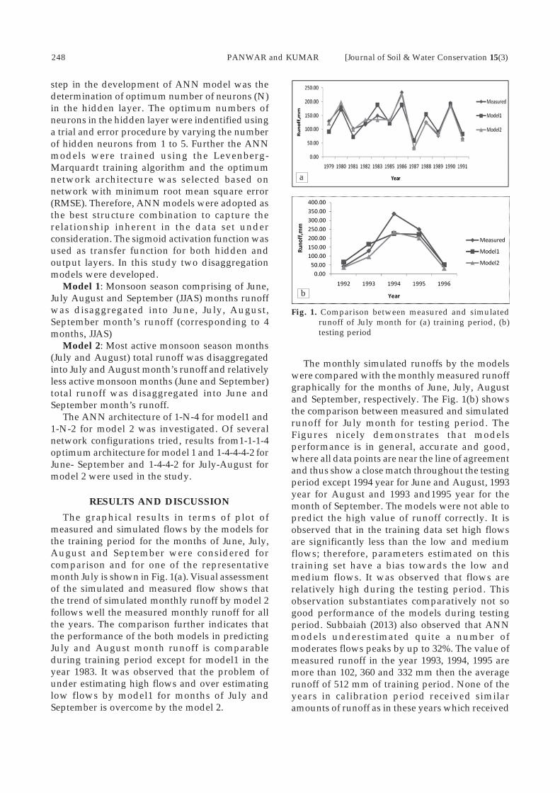
248 PANWAR and KUMAR [Journal of Soil & Water Conservation 15(3)
step in the development of ANN model was thedetermination of optimum number of neurons (N)in the hidden layer. The optimum numbers ofneurons in the hidden layer were indentified usinga trial and error procedure by varying the numberof hidden neurons from 1 to 5. Further the ANNmodels were trained using the Levenberg-Marquardt training algorithm and the optimumnetwork architecture was selected based onnetwork with minimum root mean square error(RMSE). Therefore, ANN models were adopted asthe best structure combination to capture therelationship inherent in the data set underconsideration. The sigmoid activation function wasused as transfer function for both hidden andoutput layers. In this study two disaggregationmodels were developed.
Model 1: Monsoon season comprising of June,July August and September (JJAS) months runoffwas disaggregated into June, July, August,September month’s runoff (corresponding to 4months, JJAS)
Model 2: Most active monsoon season months(July and August) total runoff was disaggregatedinto July and August month’s runoff and relativelyless active monsoon months (June and September)total runoff was disaggregated into June andSeptember month’s runoff.
The ANN architecture of 1-N-4 for model1 and1-N-2 for model 2 was investigated. Of severalnetwork configurations tried, results from1-1-1-4optimum architecture for model 1 and 1-4-4-4-2 forJune- September and 1-4-4-2 for July-August formodel 2 were used in the study.
RESULTS AND DISCUSSION
The graphical results in terms of plot ofmeasured and simulated flows by the models forthe training period for the months of June, July,August and September were considered forcomparison and for one of the representativemonth July is shown in Fig. 1(a). Visual assessmentof the simulated and measured flow shows thatthe trend of simulated monthly runoff by model 2follows well the measured monthly runoff for allthe years. The comparison further indicates thatthe performance of the both models in predictingJuly and August month runoff is comparableduring training period except for model1 in theyear 1983. It was observed that the problem ofunder estimating high flows and over estimatinglow flows by model1 for months of July andSeptember is overcome by the model 2.
The monthly simulated runoffs by the modelswere compared with the monthly measured runoffgraphically for the months of June, July, Augustand September, respectively. The Fig. 1(b) showsthe comparison between measured and simulatedrunoff for July month for testing period. TheFigures nicely demonstrates that modelsperformance is in general, accurate and good,where all data points are near the line of agreementand thus show a close match throughout the testingperiod except 1994 year for June and August, 1993year for August and 1993 and1995 year for themonth of September. The models were not able topredict the high value of runoff correctly. It isobserved that in the training data set high flowsare significantly less than the low and mediumflows; therefore, parameters estimated on thistraining set have a bias towards the low andmedium flows. It was observed that flows arerelatively high during the testing period. Thisobservation substantiates comparatively not sogood performance of the models during testingperiod. Subbaiah (2013) also observed that ANNmodels underestimated quite a number ofmoderates flows peaks by up to 32%. The value ofmeasured runoff in the year 1993, 1994, 1995 aremore than 102, 360 and 332 mm then the averagerunoff of 512 mm of training period. None of theyears in calibration period received similaramounts of runoff as in these years which received
a
b
Fig. 1. Comparison between measured and simulatedrunoff of July month for (a) training period, (b)testing period

July-September 2016] ARTIFICIAL NEURAL NETWORK 249
more values of runoff covering the years intraining.
The monthly simulated values of runoff wereplotted against the measured values for trainingand testing periods for the months of June, July,August and September for model1 and the plot forthe month of July for model 1 for training andtesting period are shown in Fig. 2(a) and Fig. 2(b),
variability. It is clear from the Table 1 that the fitof model 2 is better for all the four monthsduring training and testing period in comparisonto model 1.
Fig. 2. Comparison of measured and simulated runoff bymodel 1 of July for (a) training period, (b) testingperiod
respectively whereas for model 2 are shown in Fig.3(a) and Fig. 3(b), respectively. The values of R2
shows good fit except for the months of June andSeptember by model 1.The values of R2 of linearfit between observed and simulated runoff for themonsoon month by the two models are given inTable 1. It is clear from the Table 1 that all the valuesof coefficient of determination are in the acceptablelimit for the months of July and August in case ofmodel1, the values being higher than 0.75 fortraining and testing period. The values of R2 arenot so good for the months of June and Septemberin case of model1. The value of R2 for the monthsof June, July, August and September in case ofmodel 2 are more than 0.95 in case of trainingperiod and more than 0.65 in case of testing period.The values of R2 are higher in the months of Julyand August. The lower value of R2 in June andSeptember data series were observed due to large
a
b
Model evaluation criteriaMultiple performance criteria have been used
by the researchers to evaluate the adequacy ofANN models in simulating rainfall-runoffprocesses. A rigorous evaluation of hydrologicmodel performance should contain at least onegoodness of fit of relative error and at least oneabsolute error measure (Legates and MCcabe, 1999;Rajaee et al., 2009). The most commonly employedmeasure are Root mean squared error (RMSE),Coefficient of efficiency (CE) and correlationcoefficient (CORR). The correlation coefficient
a
b
Fig. 3. Comparison of measured and simulated runoff bymodel2 of July for (a) training period, (b) testingperiod
Table 1. Coefficient of determination (R2) of linear fitequation between observed and simulated runofffor training and testing periods
Training June July August Sept.Model 1 0.114 0.769 0.772 0.20Model 2 0.962 0.970 0.980 0.954TestingModel 1 0.710 0.870 0.636 0.279Model 2 0.708 0.982 0.950 0.649

250 PANWAR and KUMAR [Journal of Soil & Water Conservation 15(3)
ranges from 0 to 1, with higher values indicatingless error. The root mean square error is a measureof residual variance and is indicative of the modelsability to predict high flows and ranges between 0and “ with lower value corresponds to betterperformance of the model. The coefficient ofefficiency (Nash and Sulcliffe, 1970) determines therelative magnitude of the residual variancecompared to measured data variance. The valuesof coefficient of efficiency range between -” to 1.The coefficient of efficiency equal to 1 being theoptimal value representing the perfect fit. Thecoefficient of efficiency is sensitive to extremevalues and might yields suboptimal results whenthe data set contains large outliers. The equationsof RMSE, CE and CORR are as follows:
where, RPOWi and RPPWi are the observed andpredicted values for ith data set; N is the totalnumber of observations; and RPOW and RPPW arethe mean of observed and predicted values,respectively.
The results in terms of various performancesstatistics for both the models are presented in Table2. Analyzing the result it can be observed that incase of model 2 values of CORR, RMSE, CE are0.99, 9.03 and 98% for June to September and 0.97,20.99 and 94.0% for July-August during trainingperiod respectively, whereas the values are 0.87,55.57, 68.83% for June- September and 0.89, 44.42,77.64% for July-August for testing periodrespectively. Model performance of training set is
very good for both the models. The model 2 whichhad a testing correlation coefficient of 0.87 and 0.89and a testing Nash-Sutcliffe efficiency of 68.83 and77.64 performed than model 1(correlationcoefficient of 0.75 and Nash-Sutcliffe efficiency of50.44). Also the model 2 which had a testing rootmean square error of 55.57 and 44.42 was moreaccurate than model1(root mean square error of71.04). Thus on comparing values of evaluationparameters for testing set it is evident that runoffestimated by model 2 is better than model 1,therefore, it can be said when overall performancesis considered the model 2 performed better thanmodel.
CONCLUSION
This study is based in the comparative analysisfor two disaggregation models. The models wereused to predict runoff in Naula watershed ofRamganga river and their performance wereevaluated using RMSE, CE, CORR. The lower valueof RMSE and higher value of CE and CORRindicate that both the model showed goodprediction accuracy for low and medium value offlows but unable to maintain same level of accuracyfor higher value of flow. The results suggest thatANN models provide accurate estimates fordisaggregation seasonal models to monthly scale.The model 2 performed better than model 1 whenoverall performances were considered.
REFERENCES
Adamowski, J. 2007. Development of a short-term riverflood forecasting method based on wavelet analysis,J. Hydrol. 353(3–4): 247–266.
Adamowski, J. 2008a. Development of a short-term riverflood forecasting method for snowmelt drivenfloods based on wavelet and cross-waveletanalysis, J. Hydrol. 353: 247–266.
Adamowski, J. 2008b. Peak daily water demand forecastmodeling using artificial neural networks. J. WaterResour. Plan. Manage. 134(2): 119–128.
Adamowski, J. and Chan, H. F. 2011. A wavelet neuralnetwork conjunction model for groundwater levelforecasting. J. Hydrol. 407: 28–40.
Bhatt, V.K., Sharmishta Pal and Tiwari, A.K. 2011.Prediction of runoff and sediment yield for Damodarand Mayurkashi basin using artificial neutralnetwork and regression analysis. Indian J. Soil Cons.39(2):100-107.
Burain, S.J. and Durrans, S.R. 2002. Evaluation of anartificial neural network rainfall disaggregationmodel. Water Sci. Tech. 45(2):99-104
Burain, S.J. Durrans, S.R., Nix, S.J. and Pitt, R.E. 2001.Training artificial neural networks to performrainfall disaggregation. J. Hydrol. Eng. 6(1):43-51.
Table 2. Performance of models simulating runoff
Training Model 1 Model 2June-Sept. July-Aug.
CORR 0.92 0.99 0.97RMSE 33.82 9.03 20.99CE 85.44 98.00 94.04TestingCORR 0.75 0.87 0.89RMSE 71.04 55.57 44.42CE 50.44 68.83 77.64

July-September 2016] ARTIFICIAL NEURAL NETWORK 251
Burian, S.J. Durrans, S.R., Tomic, S., Pimmel, R.L. andWai, C.N. 2000. Rainfall disaggregation usingartificial neural networks. J. Hydrol Eng. 5(3):299-307.
Hornik, Kurt 1989. Multilayer feed forward networksare universal approximations. Neural Networks2(5):359-366.
Karul, C., Soyupak, S., Cilesiz, A.A., Akbay, N. andGerman, E. 2000. Case studies of neural networksin eutrophication modeling. Ecological Modelling134:145-152.
Kissi, O. 2004. River flow modeling using artificialneural networks. Journal of Hydrologic Engg. ASCE9: 60–63.
Kumar, D.N. and Raju, K.S. 2002. Temporaldisaggregation of rainfall data using artificial neuralnetworks. Proc. International conference onintegrated water Resources Management, held atNew Delhi, 2:788-795.
Legates, D.R. and MCcabe Jr.G.J.1999.Evaluating the useof goodness of fit measures in hydrologic and hydro-climatic model validation. Water Resources Research35(1): 233-241.
Nash, J. E. and Sutcliffe, J. V. 1970. River flow forecastingthrough conceptual models - 1: A discussion ofprinciples. J. Hydrol. 10: 282-290.
Nix, S.J. and Pitt, R.E. 2001. Training artificial neuralnetworks to perform rainfall disaggregation. J.Hydrol. Eng. 6(1): 43-51.
Panda, Rabindra K., Niranjan Pramanik and Biplab,Bala. 2010. Simulation of river stage using artificialneural network and MIKE 11 hydrodynamic model.Computers and Geosciences 36:735-745.
Rajaee, T., Mirabagheri, S. A., Zoufnemat-Kumani, M.,Nourani, V. 2009. Daily suspended sedimentconcentration simulation using ANN and neuro-fizzy models. Science of the total environment 407:4916-4927.
Sahoo, G.B., Ray, C. and Wade, H. F. 2005. Pesticideprediction in ground water in North Carolinadomestic wells using artificial neural networks.Ecological Modelling 183(1-2): 29-46.
Singh, R., Sharma, H.C. and Kumar, Ambrish. 2008.Artificial neural network modeling of referenceevaporation for Garhwal region of Uttarakhand.Indian J. Soil Cons. 36(3):131-135.
Srinivasulu, S. and Jain, A. 2006. A comparative analysisof training methods for artificial neural networkrainfall–runoff models. Applied Soft Computing 6:295–306.
Subbaiah, R. 2013. Application of artificial neuralnetworks for disaggregation of river seasonal inflowseries. Indian J. Soil Conservation 41(3):206-211.
Zhang, J., Murch, R.R., Ross, M.A., Ganguly A.R. andNachabe, M. 2008. Evaluation of statistical rainfalldisaggregation methods using rain-gaugeinformation for west central Florida. J. HydrologicEngg. 13(12):1158-1169.

252 SITHOLE [Journal of Soil & Water Conservation 15(3)
Journal of Soil and Water Conservation 15(3): 252-257, July-September 2016ISSN: 022-457X
Institutional dynamics of Mopane woodlandmanagement in Bulilima district of Zimbabwe
MKHOKHELI SITHOLE
Received: 14 April 2016; Accepted: 17 July 2016
ABSTRACT
The paper discusses the institutional dynamics influencing the management of Mopane woodlandsin Bulilima district of Zimbabwe. The existence of Mopani woodlands as common pool resourcesin Bulilima makes them vulnerable to over-exploitation. The institutions responsible for sustainablemanagement seem very weak. Common pool resources have been condemned as environmentallyunsustainable, economically unviable or socially anachronistic especially when they become defacto open access resources. The dismantling of local institutions in Zimbabwe came with a completedisregard of indigenous knowledge. Independent Zimbabwe inherited policies that assumedignorance among rural users. The policies currently in operation are fuzzy, inchoate, and fallingbetween local traditional governance systems which in themselves are not clearly defined and statecontrol which is so far removed from the day to day management of the resources. A questiontherefore arises on the implications of the current institutional dynamics on Mopani tree use andmanagement. The study thus attempted to establish the institutional dynamics relating to Mopanitree use and management in Bulilima profile the implications of such changes in the use behaviourof users and managers and establish the existing potential within the existing institutions formanagement of Mopani trees. As a way of gathering data this study is largely ethnographic, involvingdifferent approaches that allow for close attention such as observations, participation in the observedpractices and events, in-depth interviews, narratives and archival research. Questionnaires havealso been used to augment qualitative data. Findings indicate that at community level, there are amultiplicity of institutions and management structures with unclear mandates and jurisdictions.Power and knowledge dynamics influence processes of negotiating resource access by various actors.Although women have historically been sidelined in formal decision-making processes, they seemto be playing a key role in Bulilima largely because men are in Botswana and South Africa.
Key words: Common pool resources, Indigenous Knowledge, Resource Management
Institute of Development Studies (IDS), National University of Science and Technology (NUST), Bulawayo, Zimbabwe;Email:[email protected]
INTRODUCTION
Natural resource crisis in Africa has been largelylinked to centralized state control far removed fromthe day to day management of resources (Fabriciuset al., 2013; Eguavoen and Laube, 2010). There isan increasing consensus, evidenced by burgeoningliterature in natural resource management, that thecause of resource degradation is institutional. If weget the right rules and governance structures,natural resources will be used wisely andconservation goals will be met (Acheson, 2006).
This paper discusses institutional dynamicssurrounding the management of Mopaniwoodlands in Bulilima district of Zimbabwe. It
examines the role of local level institutions, bothformal and informal. In the case of Zimbabwe, theterm formal or modern institutional structuresrefers to governance structures of the state thatinclude the village committees (VIDCOs) and warddevelopment committees (WADCOs) that areelected” (Nemarundwe, 2003). Institutions are thusa set of informal and formal rules that facilitate andconstrain human behaviour, or define ‘the rules ofthe game’ (Bromley, 1989; North, 1990). They areconsidered to provide mechanisms wherebyindividuals can transcend social dilemmas(Acheson, 1989; Bates, 1995; Ostrom, 1990).

July-September 2016] INSTITUTIONAL DYNAMICS 253
MATERIALS AND METHODS
The study was carried out in Bulilima district,Matabeleland South province of Zimbabwe.Villages and wards are administrative units foundin communal areas of Zimbabwe. Six or sevenvillages make a ward. (Madzudzo, 1997). Thedistrict has 19 wards characterised by multiplelivelihood strategies that include small businesses,communal farms, small-scale mines and irrigationschemes, amongst others (ZIMSTATS, 2012). In thewards are villages that were used as units of study.The entire district lies within Natural Regions IVand V, which are characterised by short, variablerainfall seasons averaging generally below 400 mmper year and long dry winter periods (Vincent andTomas, 1960; Magadza, 2006; Mahati et al., 2008).The predominant tree species is ColophospermumMopane (Dye and Walker, 1980; Dube, 2008).
In Fig. 1 (a) Bulilima district is shown in one bigdistrict, Bulilimamangwe, before it was divided in2002 while in (b) Bulilima is shown as district on
its own after 2002. Bulilima and Mangwe districtswere initially part of one big district known asBulilimamangwe. In 2002 Bulilimamangwe districtwas split into three districts (Bulilima, Mangwe andPlumtree) as it was considered by the governmentof Zimbabwe to be administratively too large.Plumtree is the only urban district (Munyati, 2006).
Data sourcesThe wards selected for this study were
Makhulela and Bambadzi. Within these wards, 4villages were sampled for data collection. Thesewere Makhulela 1 and Twayitwayi from Makhulelaward and Mbimba 1 and 2 from Bambadzi ward.These areas were selected because of the exclusivedominance of Mopani resources in these wards.Selection of two wards ensured comprehensiveethnographic study in order to understandinstitutional dynamics governing the managementof Mopani woodlands. Triangulation methodswere used to verify data collected and thusimprove on its reliability and validity. Datacollection thus involved various participatorytechniques. A total of 6 focus group discussionswere conducted. Each group was composed ofbetween 8 and 12 respondents. The groupscomprised of men and women in leadershippositions, men and women who are in the naturalresources committees, ordinary members of thecommunities, a group of traditional leaders(Sobhukus and headmen) and a group of localgovernment representatives (WADCOs andVIDCOs). Key informants were identified basedon their expert knowledge about the history of thestudy area, gender, wealth, ethnicity, and age andleadership position. They provided valuableinformation on a variety of issues that includedindigenous knowledge available in managementof Mopane resources, importance of Mopaneresources to local communities, and issues ofownership and access to natural resources withinthe district. The specific informants interviewedcomprised of Bulilima Chief Executive Officer(CEO), representatives of the local governmentwhich is the District Administrator (DA),responsible for the welfare of chiefs, the VillageDevelopment Committee (VIDCO) and the WardDevelopment Committee (WADCO)representatives, Chief Makhulela, one Sobhuku,Council chairperson, officials from governmentorganisations such as Environmental ManagementAgency (EMA) and Forestry Commission, officialsfrom Non-governmental Organisations (NGOs)operating in the district and community members
Fig. 1. Map of Matabeleland South province (a) and Ward map of Bulilima district (b).

254 SITHOLE [Journal of Soil & Water Conservation 15(3)
selected because of their knowledge of the area,their position in the community and their wealthstatus in the community.
RESULTS AND DISCUSSION
Information gathered through various datacollection tools revealed that both formal andinformal institutions exist in Bulilima. Theseinstitutions result in various dimensions thatinfluence decision making and knowledgeproduction in the use and management of Mopaniwoodlands.
Formal Institutions (sometimes referred to as modern)Understanding formal institutions affecting
Mopani woodlands in Bulilima district cannot befully comprehended without discussing theinstitutional policy governing woodland resourcesin Zimbabwe. Studies on this policy (Mandondo,2000a; Sithole, 1999; Mukamuri, 1995;Murombedzi, 1991; Murphree, 1991; Mapedza,2007; Mandondo 2000; Kwashirai, 2009) indicatethat there has been a concerted effort in Zimbabweto move from state centred approaches towardsdecentralisation and participatory resourcemanagement. The idea was to empower localcommunities and encourage them to be part ofresource management within their communities.Noble as the idea has been, the reality on theground indicate that not much has been achievedin terms of ensuring local participation and naturalresource access. Formal institutions have beenhighlighted as perpetrators of the colonial systemof natural resource governance (Mapeza, 2007;Kwashirai, 2009).
The principal legislative provisions governingwoodlands in the communal areas are the ForestAct (1982), the Communal Lands Forest ProduceAct (1987) and the Rural District Councils Act(1988). Nemarundwe (2003) noted that The ForestAct of (1982) governs the establishment andprotection of state forests while the CommunalLands Forestry Produce Act (1987) prohibits thecommercialisation of forest products in allcommunal areas. The Rural District Councils Act(1988) gives district councils powers to act as thelocal planning and development authorities andenact legally binding land use and conservationby-laws that apply to areas under their jurisdiction(ibid).
The Forestry Commission, through theCommunal Lands Forestry Produce Act (1987),regulates and monitors the use of all woodland in
the district. Mopani woodland, being the dominantspecie in the area, is given special attention. Focusgroup discussions conducted in the study areasrevealed that the Forestry Commission is veryactive in enforcing its regulations on the use ofMopani woodlands. Locals are not allowed to cutdown Mopani woodlands for firewood orcommercial purposes yet outsiders can exploit anywoodland resource through use of permitsacquired either from the Forestry Commission orthe Rural District Council (RDC). This is a classiccase of government policies disempowering thelocals. During the colonial era, mining contractorsextracted wood from native reserves with theblessing of Commissioners who offered timber tothe miners at concessionary rates in affirmativerecognition of the mining industry’s contributionto overall development (Scoones and Matose,1993). The natives were not allowed similarprivileges for their own resources. In the post-colonial Zimbabwe, nothing seems to havechanged except replacing white colonisers withblack colonisers.
Outsiders who acquire permits from the RDCto exploit Mopani woodlands and other resourcesfor commercial use are allowed to harvest freely.The fees that are paid for permits accrue to the RDCand Forestry Commission and rarely do theydevelop the communities where the resourcescome from. Community members are thereforedisempowered by the national legislation in theform of the Communal Lands Forestry Produce Act(1987). The community members also highlightedthat some of their resources are extractedclandestinely late at night. There are allegationsfrom the locals that those who exploit naturalresources at night would have bribed officials fromthe police, RDC or Forestry Commission hencethey are never arrested.
Bulilima RDC also influences the managementof natural resources in the district through theCommunal Areas Management Programme forIndigenous Resources (CAMPFIRE). CAMPFIREis an organisation run by the RDC to manage thedistrict‘s natural resources for the benefit of thelocal communities. Interviews with CAMPFIREofficials and local community members revealedthat although CAPMFIRE is meant to monitor allthe resources including Mopani woodland, it onlyconcentrates on the management of elephantsbecause they have higher returns. Through theCAMPFIRE, the RDC generates income fromtrophy hunting by international hunters.According to CAMPFIRE regulations, this income

July-September 2016] INSTITUTIONAL DYNAMICS 255
should be channelled back to communities. Realityon the ground however indicates that most of therevenue collected is used by the RDC to meet itsinternal expenses. It is evident that the system ofnatural resource governance still favours the elite.Decentralisation was done to disperse power from thecentral government only to centre it on local powerfulinstitutions not the communities themselves.
Environment Conservation Committee (ECC),the Village Development Committees (VIDCOs),the Ward Development Committees (WADCOs),elected councillors and traditional authorities alsoprovide regulatory institutions that purport tomonitor the use of natural resources in the district.The ECC is a committee elected by the communitymembers to monitor the use of natural resources.This was one of the innovative ways of trying tobring the issue of resource governance to the localpeople. This committee is a brain child of the RDC.However evidence on the ground indicated thatthe committee exists only by name as it is one ofthe most passive organisations within thecommunities. It lacks necessary powers to enforceits by-laws. The committee reports to the RDC eventhough the council seemingly does not offer muchsupport. Women constitute the highest number inthis committee, a scenario that perhaps suggest itslack of influence on natural resource governancein the area.
The testimony above seems to be a commonperception among several other members of thiscommittee in the different wards. The fact that menshun this committee significantly diminishes itspowers of influence. In a patriarchal society wheremen make the rules and dominate in all forumsoutside the home, decisions about natural resourcemanagement are left to them.
VIDCOs and WADCOs are local governmententities created to foster developed at a local level.They are relevant in this discussion because overthe years they have provided a different dimensionto natural resource governance and developmentin Matabeleland region1. They owe their existenceto the Prime Minister’s directive of 1984 which alsosaw the establishment of the posts of ProvincialGovernors; the latter being appointed on loyaltyto the ruling party by the Prime Minister (Mabhena,2010). In state rhetoric VIDCOs were there topromote local decision making and should be
viewed as structures promoting democraticgovernance. In some circles however, the formationof VIDCOs was regarded as a Zimbabwe AfricanUnion Patriotic Front (ZANU PF) mechanism forcontrolling Matabeleland (Stoneman and Cliffe,1989). Madondo (2000) further concurs and arguethat the infiltration of VIDCOs and WADCOs bythe ruling ZANU-PF party has seen them carry thestigma of politically sponsored institutions thathave no clear bases in history, or mere grassrootsextensions of the ruling party. Focus groupdiscussions with the locals revealed that theseinstitutions still perform the same role as they usedto before though their activity is now lesspronounced. This could be because ZANU PF nolonger fears that serious political opposition cancome from Matabeleland region. Nevertheless,discussions showed that these two entities arepartisan in nature and in some cases are clearlyreserved for ZANU PF members. At the helm ofthe VIDCOs and WADCOs are elected councillorswho champion party agendas. Interviews with thetwo councillors from the two wards under study(one from ZANU PF and the other from Movementfor Democratic Change (MDC)) revealed thatnatural resource access purely political. Formembers of the ruling ZANU PF party, use ofMopani woodlands for whatever purpose isusually met with less ridicule by the powers thatbe compared to those perceived to be of theopposition party. However similar favours areusually denied those perceived to be of theopposition party.
Traditional institutions of chiefs, headman andkraal-head constitute a somewhat interestinginstitution in the history of natural resourcemanagement in Zimbabwe. Its legimation has beenprimary derived from customary beliefs withconsiderable support from both colonial and post-colonial governments. Traditional leaders’influence on natural resource management hasalways been at the mercy of the ruling governmentof the time. Chiefs have been constantlyempowered and disempowered to suit the policiesand agendas of the governments in power (ibid).The fact that their appointment, though customary,is influenced by the ruling party makes them anextension of state control at a local level. It is notsurprising that traditional leaders are therefore
1Village Development Committees (VIDCOs) and Ward Development Committees (WADCOs) were created as a way of controllingresources and development in Matabeleland region by the then ZANU dominated government in 80s. These Institutions were aresult of a protracted power struggle in the Matabeleland region of Zimbabwe which culminated into military operations onunarmed civilians. The operation is popularly known as Gukurahundi in Zimbabwe and resulted in the death of more than 20000 civilians (Mabhena, 2010)

256 SITHOLE [Journal of Soil & Water Conservation 15(3)
unpopular to those who do not support the rulingparty. Nevertheless, they are empowered toenforce rules and exact fines on those whoindiscriminately cut down Mopani woodlands.Group discussions however revealed that thesefines are administered in a partisan mannerdepending on which political party you areaffiliated to and are at the discretion of the chief orheadman. In most cases the collected fines aresiphoned by the RDC, a scenario that Madondo(2000) refers to as a typical case of higher levelauthorities decentralising costs but retainingcontrol of benefit. The fines rarely benefit the localcommunities of Bulilima.
Informal institutionsInformal institutions sometimes referred to as
traditional or indigenous, do exist and to a certainextent plays a key role in the sustainablemanagement of Mopani woodlands in Bulilima.While traditional leadership (chiefs, headman andkraal heads) represent an extended arm of the localgovernment that enforces all environmentalplanning and conservation by-laws, it also servesas the custodian of traditional or indigenous rulesthat govern the use of natural resources within thecommunities. Traditional management, as informalinstitutions are often referred to, are based oncustomary rights to resources. These rights basetheir legitimacy on historical existence of the localpeople who claim them within a certain geographicarea. People of Makhulela and Bambadzi claim tohave moved been pushed into these areas by thewhite colonial government in the early 1950s. Theyhave since developed ways of interacting with theirecological environment, which is dominated byMopani woodland species. Over the year they havelearnt to sustainably use the woodland. In one ofthe focus group discussion with women, it wasrevealed that Mopani tree commands some respectwithin the communities because it provides otherproducts such as Mopani worms, which are muchmore valuable. Almost every year, the localsharvest Mopani worms from Mopani woodlands.The worms are a significant source of livelihood.There is a belief amongst the community membersthat Mopani worms are a gift from the ‘Gods‘ hencein every Mopani worm season, a few elderly peoplechosen to take some of the worms to the shrineknown as Daka. It is here that they thank theancestral spirits for providing them with food andthey also ask for more rains. Daka therefore is avery important institution in the management ofMopani resources. It is imperative that policies
aimed at natural resource management at a locallevel consider such traditional institutions sincethey influence local people‘s perceptions onselection and integration of externalities into thelocal practices (Yelsang, 2014).
Interviews with Chief Makhulela centred ontraditional beliefs and norms as a way ofconserving natural resources in the area. The chiefbelieved that local people with their roots in thearea generally respect and understand thatresources such as big Mopani trees should not becut unless for very special purposes. Outsiders,especially those who have been recently resettledunder the Fast Track Land Reform Programme(FTLRP) do not have such respect for the trees.FTLRRP is a form of land redistribution inZimbabwe which began in July 2000 through theLand Reform and Resettlement Programme Phase11. It envisaged acquiring 5 million hectares andresettling new farmers on all acquired land(Murombedzi, 2005; Barry, 2004; Hammar andRaptopoulos, 2003).
The newly resettled locals, who live in nearbyvillages, seem to be protected by institutions morepowerful than the traditional institutions followedby the locals. Perhaps it is a question of customaryrights being seen as inferior to statutory rights. Thediscussions revealed that people fromresettlements indiscriminately cut down treesdisrespecting the social co-existence between thelocals in Mbimba and their ecology.
CONCLUSION
The study analysed institutional dynamicssurrounding the management of Mopaniwoodlands in Bulilima district of Zimbabwe. Thefocus was on two wards, Makhulela and Bambadzi,because they have an abundance of Mopaniwoodland. Makhulela 1 and Mbimba were selectedas villages where data was collected. The studyrevealed that the management of natural resourcesand in this case Mopani woodland is influencedby both formal and informal institutions. The twosets of institutions do not always function smoothlyand in most instances formal institutions tend tooverride traditional institutions to the detrimentof the resources. It was established that generallyformal institutions are more powerful as they enjoypolitical backing. However their power does nottranslate to sustainable management of Mopaniwoodland as local people who have alwayssurvived within their woodlands felt that theyalways had the right to use the resources as thecommunity deems fit. Conflicts were inevitable

July-September 2016] INSTITUTIONAL DYNAMICS 257
resulting in general unpopularity of the Chiefs inthis area. Chiefs are seen as oppressors because partof their duty is to fine those they consider to bebreaking environmental laws as prescribed in thecouncil by-laws.
It is however important to note that whilemodern institutions are there to stay, resourcesustainability can be enhanced if there is fusion ofideologies from both formal and informal settings.Local institutions still have the opportunity whenit comes to natural resource management. This isso because, the use of customary laws by traditionalinstitutions is relevant to the people because theystill believe in them. Communities from both wardsunder study believe that appeasing the ‘Gods‘ bygiving them some of their harvest, be it crops orMopani worms, brings more rain and more resources.
REFERENCES
Acheson, J.M. 2006. Institutional failure in resourcemanagement. Annual Review of Anthropology 35: 117-134.
Acheson, J. M. 1989. Management of Common PropertyResources. In Platter, S. (Ed). Economic Anthropology.Stanford University Press. Stanford, pp 351-379.
Bates, R.H. 1995. Social Dilemmas and RationalIndividuals: An Assessment of the newInstitutionalism. In: J. Harris, J. Hunter and C.M.Lewis (eds). The New Institutional Economics and ThirdWorld Development. Routledge. London, pp 27-48.
Barry, H. D. 2004. The Past is the Future. Weaver Press,Harare.
Bromley, D. W. 1991. Environment and Economy: Propertyrights and public policy. Blackwell Publishers,Cambridge.
Bromley, D. W. 1989. Economic Interests and Institutions:The Conceptual Foundations of Public Policy, BasilBlackwell, New York.
Bromley, D.W. (ed). 1992. Making the Commons Work:Theory, Practice and Policy. ICS Press, San Francisco.
Dube, C. 2008. The Impact of Zimbabwe‘s drought policyon Sontala Rural Community in Matabeleland SouthProvince . Unpublished MSc dissertation.Stellenbosch University. Unpublished.
Dye P. J., and Walker, B.H. 1980. Vegetation–environmentrelations on sodic soils of Zimbabwe-Rhodesia. TheJournal of Ecology 68(2): 589-606.
Eguavoen, I. and Laube, W. (Eds) 2010. Negotiating LocalGovernance. Natural Resource Management at theinterface of communities and the state. ZETDevelopment Studies. Deutsche Bibliothekpublishers.
Fabricius, C., Koch, E., Turner, S. and Magome, H. (Eds.).2013. Rights resources and rural development:Community-based natural resource management inSouthern Africa. Routledge.
Hammar, A. and Raftopoulos, B. 2003, Zimbabwe’s:Unfinished Business Rethinking Land, State and Nationin the Context of Crisis, Weaver Press, Harare.
Kwashirai, V. C. 2012. Environmental History of Africa.Encyclopedia of Life Support Systems.
Mabhena, C. 2010. Visible Hectares, Vanishing Livelihoods’:A case of the Fast Track Land Reform and ResettlementProgramme in southern Matabeleland-Zimbabwe,Doctoral dissertation, University of Fort Hare.
Madzudzo, E. 1997. Communal Tenure, MotivationalDynamics and Sustainable Wildlife Management inZimbabwe. Zambezia 24(2): 1-12.
Magadza, S.N. 2006. Empowerment, mobilisation andinitiation of a community driven project: womenand the marula. Agricultural Economics Review 7(1):1-15.
Mahati, S. T., Munyati, S. and Gwini, S. 2008. Situationalanalysis of orphaned and vulnerable children in eightZimbabwean districts. HSRC Press.
Mandondo, A. 2000. Situating Zimbabwe’s natural resourcegovernance systems in history (No. 32). Centre forInternational Forestry Research, Bongor.
Mandondo, A. 2000a. Situating Zimbabwe’s NaturalResource Governance Systems in History. Center forInternational Forestry Research Occasional PaperNo. 32. CIFOR. Bogor.
Mapedza, E. 2007. Keeping CAMPFIRE going: Politicaluncertainty and Natural Resource Management inZimbabwe. International Institute for Environmentand Development, London.
Munyati, S., Rusakaniko, S., Mahati, ST., Mupambireyi,P. F., Chibatamoto, P.,and Chandiwana, B. 2006. Aqualitative assessment of vulnerable children in twoZimbabwean districts. HSRC Press, Cape Town, SouthAfrica.
Murombedzi, J.C. 1991. Decentralising Common PropertyResources Management: A Case Study of theNyaminyami District Council of Zimbabwe’s WildlifeManagement Programme. IIED Paper No. 30. London.
Murombedzi, J. 2005. Environment and SustainableDevelopment in Zimbabwe, CASS Publications,Harare.
Murphree, M. W. 1991. Communities as Institutions forResource Management Institutions. Centre for AppliedSocial Sciences, University of Zimbabwe. Harare.
Nemarundwe, N. 2003. Negotiating Resource Access.Institutional arrangements for woodlands and water usein southern Zimbabwe . PhD thesis, SwedishUniversity of Agricultural Sciences, Uppsala.
North, D. 1990. Institutions, Institutional Change andEconomic Performance. Cambridge University Press.Cambridge.
Ostrom, E. 1990. Governing the Commons: The Evolutionof Institutions for Collective Action. CambridgeUniversity Press, New York.
Vincent, V., Thomas, R. G. and Staples, R. R. 1960. Anagricultural survey of Southern Rhodesia. Part 1. Agro-ecological survey. An agricultural survey ofSouthern Rhodesia.
Yelsang, F.D. 2013. Sustainability of natural resourcemanagement: where do informal and formalstrategies converge? Development Country Studies3(8): 36-44.
258 NAGARAJA et al. [Journal of Soil & Water Conservation 15(3)
Journal of Soil and Water Conservation 15(3): 258-264, July-September 2016ISSN: 022-457X
Soil carbon stocks in natural and man-made agri-horti-silvipastural land use systems in dry zones of Southern India
M.S. NAGARAJA1, A.K. BHARDWAJ2 *, G.V.P. REDDY3,V.R.R. PARAMA3 and B. KAPHALIYA4
Received: 16 May 2016; Accepted: 6 August 2016
ABSTRACT
A study was undertaken to assess the soil carbon stocks in 0-50 cm soil depth, under natural andman-made land use systems in the eastern dry zones of Karnataka in India. The carbon (C) stocksin soils ranged from 26.46 t ha-1 in dry land agricultural systems (without manure) to 89.20 t ha-1 ina mixed forest. Among natural systems, mixed forest (89.20 t ha-1) and ungrazed grassland (71.78 tha-1) recorded higher levels of C stock than other systems, while grazing in grassland and litterremoval in teak plantations correlated to reduced carbon stocks to 39.32 and 32.74 t ha-1, respectively.Intensively managed horticultural systems namely, grapes plantation (85.52 t ha-1) and pomegranateplantation (78.78 t ha-1) maintained higher levels of C stock. However, agricultural systems recordedmoderate to lower levels. Total carbon stocks in top 0-50 cm soils of agricultural systems was in theorder: irrigated lands with manure application (52.77 t ha-1) > irrigated lands without manureapplication (44.47 t ha-1) > dry lands with manure application (37.79 t ha-1) > dry lands withoutmanure application (26.46 t ha-1). It was observed that adoption of appropriate soil and cropmanagement practices such as conservation tillage, good irrigation, incorporation of crop residuesand application of manure etc. could enhance soil C pool by reducing existing carbon loss andpromoting C accumulation in the soil.
Key words: Soil carbon, land use systems, residue recycling, forest, horticulture, grassland.
1Associate Professor, College of Horticulture, University of Horticultural Sciences, Bagalkot-587102, Karnataka; 2Senior Scientist,ICAR-Central Soil Salinity Research Institute, Karnal-132001, Haryana; 3Research Scholar, Department of Soil Science, Universityof Agricultural Sciences, Bangalore -587165, Karnataka; 4Research Associate, ICAR-CSSRI, Karnal, Haryana, India; E-mail:[email protected]
INTRODUCTION
Evidences are mounting that better soilmanagement practices could contributesubstantially to the mitigation of atmosphericcarbon dioxide emissions (Yan et al., 2005; Xu et al.,2011). Conversion of natural ecosystems toagriculture in the last century has contributed tothe extent of one sixth of atmospheric greenhousegases through reduction in standing (vegetation)carbon (C) and soil C stocks (Tilman et al., 2002).
Soil C constitutes a major pool in global C cycle(Scharlemann et al., 2014). It is estimated that theSoils contain about 1550 Pg organic carbon and 950Pg inorganic carbon in the upper 1m of soil layer(Lal, 2004). It is also well established that thesetrends could be reversed through management andland use changes (Robertson et al., 2015). Thecarbon stored in soil of an ecosystem is controlledby the quality and quantity of biomass added and
its loss through decomposition. The rate of Caccumulation or loss from soil is determined bythe quantity of recyclable biomass-C, temperature,rainfall, soil moisture content and managementinduced disturbances (Delon et al., 2015; Mills etal., 2014; Bhardwaj et al., 2016). The carbon contentis generally higher in the surface layer than deepersub-surface layers as much of the plant and animaldead material reach the surface directly. Finally,the rate of C accumulation in soil is significantlycontrolled by the net balance between inputs andoutputs per unit time (Fang et al., 2015). Adoptionof suitable management practices viz., conservationtillage, good irrigation practices, incorporation ofcrop residues, manure application etc. can enhancesoil C pool by decreasing C losses and encouragingits sequestration in soil (Jarecki and Lal, 2003;Bhagat et al., 2003). Important soil functions thatare affected by agricultural land use are primary

July-September 2016] SOIL CARBON STOCKS 259
productivity, carbon storage and cycling, nutrientscycling and water purification and regulation(Bouma et al., 2014; Schulte et al., 2014).
Thus, soil can act as a large terrestrial sink ofatmospheric CO2 but the storage of C in soil isaffected by the land use: crops/plant species, tillageand crop management, residue removal andincorporation and irrigation practices. Knowingthe effect of these variables helps in land useplanning as well as in accounting of C stocks atregional level. Keeping these in view, a study wasundertaken in the Eastern dry zone of Karnatakain India to assess the soil carbon stocks (0-50 cmsoil) under different land use systems, both naturaland manmade, comprising of forests, grasslands,horticultural and agricultural systems.
MATERIALS AND METHODS
Study Area and land use systemsThe soils of the study area originated from
granite and gneiss, and are classified as Kaolinitic,isohyperthermic, belonging to Typic Kandiustalf.The study area is situated at a latitude of 12o 58’ Nand longitude of 77o 35’ E at an elevation of about930 MSL. The climate that prevailed was coolsummer and warm winter with bimodaldistribution pattern and a mean annual rainfall of844 mm.
The forest systems comprised of mixed forest(>20 tree species) and a teak plantation. Thegrassland systems studied consisted of two naturalgrassland patches with and without grazing, andone man made napier patch. Horticultural systemsincluded mango plantations with complete in situlitter turnover, and intensively managed grapesand pomegranate plantations. Agriculturalsystems comprised of both irrigated and drylandsystems, with and without farmyard manure(FYM) along with recommended doses offertilizers. Detailed descriptions of each land usesystem are given in Table 1.
Quantification of biomass produced and recycledQuantity of biomass produced, removed and
recycled were determined separately for each landuse system. In grassland systems, the above groundbiomass was harvested from one square meterwhile the below ground biomass was removed bydigging and the roots were washed thoroughly anddried. Quantity of biomass was expressed on dryweight basis. Similarly, in grazed and napiergrasslands the stubble and root biomass left aftergrazing/harvest were quantified. Biomassquantification was restricted only to annual litterturnover in forest systems as the methodology forannual root biomass estimations are not available.The litter samples were collected from one squaremeter area at a regular interval to get the annual
Cultivation (C); Irrigation (IR); Weedicide (W); Pesticides (P); Fertilization (F); Manuring (M); Harvesting (H); Grazing (G).
Land use systems Vegetation System Management Practices Biomass RemovedGrassland Systems
Ungrazed Grasses Natural None NoneGrazed Grasses Natural G GrassesNapier Grasses Manmade C, F, H Grasses
Forest SystemsMixed Trees, Bushes Natural None NoneTeak Teak Manmade Litter Removal Litter
Horticultural SystemsGrapes Grapes Manmade C, IR, P, W, F, M, H Fruits + CanePomegranate Pomegranate Manmade C, IR, P, W, F, M, H FruitsMango Mango Manmade C, P, F, H Fruits
Agricultural SystemsIrrigated Plots Finger Millet Manmade C, IR, M, F, H, W, P Grain + Straw(Fert. + FYM) + CornIrrigated Plots Finger Millet + Manmade C, IR, F, H, W, P Grain + Straw(Only Fert.) CornDryland Plots Finger Millet Manmade C, M, F, H, W, P Grain +Straw(Fert. + FYM)Dryland Plots Finger Millet Manmade C, F, H, W, P Grain + Straw(Only Fert.)
Table 1. Details of the studied land use systems.

260 NAGARAJA et al. [Journal of Soil & Water Conservation 15(3)
turnover (Shylaja et al., 1993).The biomass produced in horticultural systems
was quantified by collecting the litter samples fromone square meter and recording the annual fruityield. Annual root biomass was not estimated inthese systems, as the destructive method ofsampling would result in large economic losses.In agricultural systems, the quantity of fodder andgrain produced were used from the actual yielddata and the biomass left in the field after theharvest of the crop was determined as detailed ingrasslands.
Soil sampling and estimation of soil-C stocksThree sampling sites were chosen for each land
use system. In each site, soil samples were collectedfrom 3 different spots at 0-15, 15-30 and 30-50 cmdepths and the samples were pooled to getcomposite samples for each depth separately.These composite soil samples (depth wise) wereair dried and passed through 2 mm sieve for furtheranalyses. The soil present in 0-50 cm layer wasdetermined by measuring the bulk density of soilsfor three depths separately and the carbon contentfor the collected soil samples were determined byadopting modified Walkley and Black (1934) wetoxidation method. Soil carbon stock was estimatedby considering the soil bulk density and finefractions.
Statistical analysisAll parameters were tested using a one-way
analysis of variance (ANOVA) and separation ofmeans was subjected to Tukey’s honestlysignificant difference test (Steel and Torrie, 1960).Correlation analysis was conducted to identifyrelationships between the measured parameters.All tests were performed at 0.05 significance level.
RESULTS AND DISCUSSION
Biomass produced and recycledThe data on the quantity of biomass produced,
removed and recycled annually among differentland uses systems are given in Table 2.
Biomass Production: Among 12 different landuse types, pomegranate orchards recorded the leastbiomass production with 3.6 t ha-1, while irrigatedagricultural systems with two crops of finger milletand maize, supplemented with manures andfertilizers, produced 30.0 t ha-1 of biomass. Ingrassland systems, the annual biomass productionranged from 6.0 - 13.8 t ha-1 with least productionin grazed land and the highest in napier grassland.Irrigated agricultural systems recorded very highbiomass production compared to dryland systems.The moisture limitations in dryland restricted thecropping to only one crop per year, which was able
* Biomass produced included litter, fruit, grain, straw and root; ‡ biomass removed included grain, fodder, litter and fruit; § Residuebiomass recycled included roots and stubble in annuals and only litter (leaves + twigs) in perennial trees; † Net organic matter (OM)recycled = Residue BM recycled + FYM added; # Below ground BM produced / recycled not considered.
Land use system *Biomass ‡Biomass §Residue BM FYM †Net OMProduced Removed Recycled added Recycled
Grassland SystemsUngrazed 6.7 0.0 6.7 0.0 6.7Grazed 6.0 3.5 2.5 0.0 2.5Napier 13.8 7.0 6.8 0.0 6.8Forest SystemsMixed# 6.7 0.0 6.7 0.0 6.7Teak# 5.2 4.2 1.0 0.0 1.0
Horticultural SystemsGrape# 7.2 7.1 0.1 50.0 50.1Pomegranate# 3.6 2.4 1.2 12.5 13.7Mango# 5.4 1.0 4.4 0.0 4.4
Agricultural SystemsIrrigated (FYM + Fert.) 30.0 20.0 10.0 15.0 25.0Irrigated (Fert. Alone) 24.9 17.5 7.5 0.0 7.5Dryland (FYM +Fert.) 17.1 10.5 6.6 10.0 16.6Dryland (Fert. Alone) 8.2 3.4 4.8 0.0 4.8
Table 2. Quantity of in-situ and ex-situ annual biomass turnover (t ha-1) among different land use systems.

July-September 2016] SOIL CARBON STOCKS 261
to produce 8.2 and 17.1 t ha-1 of biomass. The litterbiomass (fallen leaves and stems) ranged from 3.6- 7.2 t ha-1 among land use systems with perennialtrees. Natural mixed forest recorded 7.2 t of litterbiomass, while teak plantations produced 5.2 t oflitter per hectare. In case of horticultural systems,the above ground biomass produced in grape andmango orchards were 7.2 t ha-1 and 5.4 t ha-1,respectively.
Residue biomass recycledLand management practices adopted in a given
system determine extent of the biomass recycling.There was no removal of biomass in the non-grazedgrasslands and mixed forests, and hence, all thebiomass produced was allowed to recycle. Whilein grazed land, 3.5 t ha-1 of grass biomass wereremoved as fodder and hence, only 2.5 t ha-1 ofbiomass was allowed to recycle in the form ofstubble and roots. Among irrigated agriculturalsystems, biomass was removed (grain and fodder)to an extent of 20.0 t ha-1 in fertilizer and FYMtreated plots and 17.5 t ha-1 in no-FYM plots (onlyfertilizer). Thus, the quantity of biomass allowedto recycle was 10.0 and 7.5 t ha-1, respectively.However, the moisture limitations in drylandrestricted the turnover to 6.6 and 4.8 t ha-1,respectively in plots with fertilizer plus manureand fertilizer alone plots. Among tree basedperennial systems, mixed forest recorded an in situbiomass turnover of 6.7 t ha-1. Litter removal inteak plantations, to prevent fire damages, resultedin a biomass turnover of mere 1.0 t ha-1. Extractionof fruits was the major source of biomass removalin horticultural systems except in grapes, wherethe biomass was also removed in the form of canesand leaves during pruning operations. Thus, themanagement practices adopted in a given systemand the quantity of biomass recycled is likely tohave an influence on the net soil carbon stocks.
Net organic matter recycledIn manmade agricultural and horticultural
systems, unlike the natural ones, organic matterwas added in the form of compost/manure tomaintain yield and quality. Thus, the net organicmatter recycled would be the sum of residuebiomass and manure. The net organic matterrecycled was as high as 50.1 t ha-1 in grape orchardand it was low in pomegranate plots with a netturnover of 13.7 t ha-1. However, there was noaddition of manure to mango and thus the biomassrecycled was equal to the net organic matterrecycled. In FYM treated agricultural systems,
irrigated lands recorded a net biomass turnover of25.0 t ha-1 while, dryland system recorded 16.6 tha-1. However, the net biomass recycled among no-FYM plots (only fertilizer applied), in both irrigatedand dryland agricultural systems, were equal tothat of residue biomass recycled. Application oforganic sources enhances all the pools of soil carbon(Khursheed et al., 2013) indicating recycling oforganic matter. Similarly, the net biomass recyclingwas unchanged in ungrazed grassland and forestsystems as there was no addition of organic matterfrom external sources.
Soil carbon stocksThe data on seasonal changes in soil organic-C
under different land use systems at various depthsare given in Table 3. The amount of total soil carbonstocks present in 0-50 cm of soil layer is depicteddiagrammatically in Fig. 1. The surface soils (0-15cm) of all land use systems in all the three seasonsrecorded highest soil organic-C. In general, the soilorganic-C was higher in winter season and lowerin summer.
Carbon present in these soils is mostly organicin nature and is present in the form of humus coatover soil particles. It decreased with depth in allthe treatments and it differed significantly amongtreatments as well as seasons (Table 3). There areno records of elemental carbon in these soils as
Fig. 1. Soil carbon stocks among different land use systems.UG = Ungrazed grasses, GG = Grazed grasses, NG =Napier grass, MF = Mixed forest, TF = Teak Forest, GH =Horticultural plantation-Grape, PH = Horticulturalplantation-Pomegranate, MH = Horticultural plantation-Mango, IR-1 = Irrigated agricultural system with FYM andfertilizer, IR-2 = Irrigated agricultural system with fertilizeralone, DL-1 = Dryland agricultural system with FYM andfertilizer, and DL-2 = Dryland agricultural system withfertilizer alone.

262 NAGARAJA et al. [Journal of Soil & Water Conservation 15(3)
there are no natural deposits of coal/coke.Higher level of carbon was recorded in mixed
forest patches (2.91 %) during rainy season andlowest was observed during summer in drylandagricultural plots with no FYM. Among thesystems, based on mean depths and season, theungrazed control plot (1.24 %), grapes (1.36 %),pomegranate orchards (1.24 %) and mixed forests(1.70 %) systems recorded more than 1.0 % of soilorganic-C. Moderate levels of soil organic-C wereobserved among other systems except teakplantations (0.46 %) and dryland plots receivingonly fertilizers (0.38 %). The variations in soilorganic-C among different land use systems wouldbe attributed to the net biomass turnover and landmanagement practices adopted in the system (Postand Kwon, 2000). Influence of managementpractices and biomass addition/turnover on soilcarbon stocks is well documented (Liao et al., 2010).
The amount of soil carbon present in the formof humus is a function of bulk density and soilorganic-C content. It was determined using the soilvolume and its corresponding soil organic-Ccontents. The amount of carbon stored in the top0-50 cm soil layer ranged from 32.7 t ha-1 in teakplantations to 89.5 t ha-1 in mixed forest. Similarly,the soil carbon stock in ungrazed grassland (71.8 tha-1) was higher than grazed (39.3 t ha-1) and napier(42.5 t ha-1) grasslands. The data also indicate thatthe quantity of carbon stored in horticulturalsystems was much higher than the disturbed forestand grassland ecosystems. The amount of soil
carbon present in top 0-50 cm soil layer was 85.5,78.8 and 51.6 t ha-1 in grapes, pomegranate andmango systems respectively. Interestingly, the soilcarbon stocks was almost near to that of disturbednatural systems and lesser than horticulturalsystems. Irrigated agricultural systems had stored52.8 t ha-1 in FYM and fertilizer treated plotscompared to 44.5 t ha-1 in fertilizer alone treatedplots. Similar trend was observed in drylandagricultural systems with much lesser quantitiesof humus carbon. The corresponding values indryland agricultural systems were 37.8 t ha-1 (withmanure and fertilizer) and 26.5 t ha-1 (with fertilizeralone).
Soil organic-C of any ecosystem is determinedby the quality and quantity of C-inputs throughbiomass addition (Liu et al., 2014) and its lossthrough decomposition (Zhu et al., 2014, Toosiet al., 2014). Larger the biomass turnover higherwould be the soil organic carbon. Large carbonstocks were observed in natural forest andungrazed grasslands and it could be attributed tohigh biomass turnover and no disturbances.However, manmade napier and grazed grasslandsrecorded much lower carbon stocks than ungrazedplots. Reduction in soil organic-C in napiergrasslands could be due to regular cultivationpractices adopted (Panagos et al., 2015) and highersoil temperature as the surface was not coveredmost of the time (Hopkins et al., 2014). Litterremoval in teak plantation to prevent fire damagesmight have severely reduced the soil carbon stocks.
Table 3. Seasonal changes in soil organic carbon (per cent) under different land use systems.
Land use system Winter Summer RainySOIL ORGANIC CARBON (%)
Grassland SystemsUngrazed 1.27 1.28 1.17Grazed 0.56 0.52 0.60Napier 0.62 0.71 0.52
Forest SystemsMixed 1.85 1.58 1.68Teak 0.38 0.56 0.45
Horticultural SystemsGrape 1.41 1.39 1.28Pomegranate 1.32 1.40 1.01Mango 0.67 0.89 0.69
Agricultural SystemsIrrigated (FYM +Fert) 0.96 0.59 0.79Irrigated (Fert. Alone) 0.74 0.51 0.64Dryland (FYM +Fert) 0.62 0.52 0.54Dryland (Fert. Alone) 0.35 0.38 0.39
The values indicated are the mean of three depths.

July-September 2016] SOIL CARBON STOCKS 263
Agroforestry system results in leaf litter fall thatrecycles the C as well as nutrients to the soil(Solanki and Arora, 2015). This suggests that thecultivation and removal of surface cover wouldreduce soil carbon through enhanced decompositionrates (Sayer, 2006; Leff et al., 2012; Fekete et al.,2014).
CONCLUSION
The carbon preserved in the form of humus onsoil particles could be used effectively as a meanto sequester atmospheric CO2 and hence inmitigating global warming effects. The amount ofcarbon stored is determined by the quality andquantity of biomass added and its loss throughdecomposition. Deforestation, expansion ofagriculture, shifting cultivation, irrigation etc.would lead to oxidation of organic matter in soil.These processes would result in CO2 release,leading to increased concentration of CO2 in theatmosphere. However, substantial carbonaccumulation can also occur in soil with increasein biomass turnover and reduction in mechanicaldisturbances. Thus, adoption of conservationtillage, good irrigation practices, crop residueincorporation, manure application etc. couldenhance soil carbon to a great extent by decreasingthe loss of existing carbon mass and encouragingcarbon accumulation. Results of the present studyclearly indicate that there is a great scope tomitigate atmospheric CO2 through better landmanagement practices.
ACKNOWLEDGEMENT
We acknowledge the help of the Department ofSoil Science, University of Agricultural Sciences,Bangalore and Centre for Ecological Sciences,Indian Institute of Science, Bangalore, forproviding requisite facilities to carry out thisresearch.
REFERENCES
Bhagat, R.M., Bhardwaj, A.K. and Sharma, P.K. 2003.Long-term effect of residue management on soilphysical properties, water use and yield of rice innorth-western India. Journal of the Indian Society ofSoil Science 51(2): 111-117.
Bhardwaj, A.K., Nagaraja, M.S., Srivastava, S., Singh,A.K. and Arora, Sanjay 2016. A framework foradaptation to climate change effects in salt affectedagricultural areas of Indo-Gangetic region. Journalof Soil and Water Conservation 15(1): 22-30.
Bouma, J. 2014. Soil science contributions towardssustainable development goals and their
implementation: linking soil functions withecosystem services. J. Plant Nutr. Soil Sci 177(2):111–120.
Delon, C., Mougin, E., Serca, D., Grippa, M., Hiernaux,P., Diawara, M., Lacaux, C.G. and Kergoat, L. 2015.Modelling the effect of soil moisture and organicmatter degradation on biogenic NO emissions fromsoils in Sahel rangeland (Mali) C. Biogeosciences 12:3253–3272.
Fang, X.M., Chen, F.S., Wan, S.Z., Yang, Q.P. and Shi,J.M. 2015. Topsoil and deep soil organic carbonconcentration and stability vary with aggregate sizeand vegetation type in subtropical China. PLoS ONE10(9): e0139380. doi:10.1371/journal.pone.0139380.
Fekete, I., Kotroczó, Z., Varga, C., Nagy, P.T., Várbíró,G., Bowden, R.D., Tóth, J.A. and Lajtha, K. 2014.Alterations in forest detritus inputs influence soilcarbon concentration and soil respiration in aCentral-European deciduous forest. Soil Biol. Biochem74:106–114.
Hopkins, F.M., Filley, T.R., Gleisner, G., Lange, M., Top,S.M. and Trumbore, S.E. 2014. Increasedbelowground carbon inputs and warming promoteloss of soil organic carbon through complementarymicrobial responses Francesca. Soil Biology &Biochemistry 76: 57-69.
Jarecki, M.K. and Lal, R. 2003. Crop management forsoil carbon sequestration. Critical Reviews in PlantSciences 22(5): 471–502.
Khursheed, S., Arora, Sanjay and Ali, T. 2013. Effect oforganic sources of nitrogen on rice (Oryza sativa) andsoil carbon pools in Inceptisols of Jammu.International Journal of Environmental Pollution andSolutions 1:17-21.
Lal, R. 2004. Soil carbon sequestration impacts on globalclimate change and food security. Science 204:1623-1627.
Leff, J.W., Wieder, W.R., Taylor, P.G., Townsend, A.R.,Nemergut, D.R., Grandy, A.S. and Cleveland, C.C.2012. Experimental litterfall manipulation driveslarge and rapid changes in soil carbon cycling in awet tropical forest. Global Change Biol 18:2969-2979.
Liao, C., Luo, Y., Fang, C. and Li, B. 2010. Ecosystemcarbon stock influenced by plantation practice:Implications for planting forests as a measure ofclimate change mitigation. PLoS ONE 5(5): e10867.doi:10.1371/journal.pone.0010867.
Liu, C., Lu, M., Cui, J., Li, B., Fang, C. 2014. Effects ofstraw carbon input on carbon dynamics inagricultural soils: a meta-analysis Glob Chang Biol20(5):1366-1381.
Mills, R.T.E., Gavazov, K.S., Spiegelberger, T., Johnson,D. and Buttler, A. 2014. Diminished soil functionsoccur under simulated climate change in a sup-alpine pasture, but heterotrophic temperaturesensitivity indicates microbial resilience. Science ofThe Total Environment 473–474:465–472.
Mishra, V.K., Srivastava, S., Bhardwaj, A.K., Sharma,D.K., Singh, Y.P. and Nayak, A.K. 2015. Resourceconservation strategies for rice wheat croppingsystems on partially reclaimed sodic soils of the Indo

264 NAGARAJA et al. [Journal of Soil & Water Conservation 15(3)
Gangetic region, and their effects on soil carbon.Natural Resources Forum, 39 (2): 110-122.
Panagos, P., Borrelli, P., Meusburger, K., Alewell, C.,Lugatoa, E. and Montanarellaa, L. 2015. Estimatingthe soil erosion cover-management factor at theEuropean scale. Land Use Policy 48:38–50.
Post, M.W. and Kwon, K.C. 2000. Soil CarbonSequestration and Land-Use Change: Processes andPotential. Global Change Biology 6:317–328.
Robertson, F., Armstrong, R., Partington, D., Perris, R.,Oliver, I., Aumann, C., Crawford, D. and Rees, D.2015. Effect of cropping practices on soil organiccarbon: evidence from long-term field experimentsin Victoria, Australia. Soil Research 53(6):636-646.
Sayer, E.J. 2006. Using experimental manipulation toassess the roles of leaf litter in the functioning offorest ecosystems. Biol. Rev. Camb. Philos. Soc. 81:1– 31.
Scharlemann, J.P.W., Tanner, E.V., Hiederer, R. andKapos, V. 2014. Global soil carbon: understandingand managing the largest terrestrial carbon pool.Carbon Management 5(1):81–91.
Schulte, R.P.O., Creamer, R., Donnellan, T., Farrelly, N.,Fealy, R., O’Donoghue, C. and O’hUallachain, D.2014. Functional land management: a framework formanaging soil-based ecosystem services for thesustainable intensification of agriculture. Environ.Sci. Policy 38:45–58.
Shylaja, R., Nagaraja, M.S. and Indira, G. 1993. Landuse and soil studies: Field manual for monitoringland and soil. Center for Environment Education
(CEE), South Regional Center, Bangalore.Solanki, R. and Arora, S. 2015. Leaf litter dynamics in
Agroforestry system affecting microbial activity inSaline Soils. Journal of the Soil and Water Conservation14(4): 332-339.
Steel, R.G.D. and Torrie, J.H.1960. Principles andprocedures of statistics. McGraw-Hill, New York,New York, USA.
Toosi, A.T., Christensena, B.T., Hutchings, N.J., Vejlina,J., Kätterer, T., Glendiningc, M. and Olesena, J.E.2014. C-TOOL: A simple model for simulatingwhole-profile carbon storage in temperateagricultural soils. Ecological Modelling 292:11-25.
Tilman, D., Cassman, K.C., Matson, P.A., Naylor, R. andPolasky, S. 2002. Agricultural sustainability andintensive production practices. Nature 418: 671-677.
Xu, S., Shi, X., Zhao, Y., Yu, D., Li, C., Wang, S., Tan,M. and Sun, W. 2011. Carbon sequestration potentialof recommended management practices for paddysoils of China, 1980–2050. Geoderma 166 (1): 206-213.
Yan, X.Y., Yagi, K., Akiyama, H. and Akimoto, H. 2005.Statistical analysis of the major variables controllingmethane emission from rice fields. Global Change Biol11: 1131–1141.
Zhu, L., Hu, N., Yang, M., Zhan, X. and Zhang, Z. 2014.Effects of different tillage and straw return on soilorganic carbon in a rice-wheat rotation system. PLoSOne 9(2): e88900. Published online 2014 Feb 20. doi:10.1371/journal.pone.0088900.

July-September 2016] WATERSHED BASED DRAINAGE 265
Journal of Soil and Water Conservation 15(3): 265-272, July-September 2016ISSN: 022-457X
Watershed based drainage morphometric analysisusing Geographical Information System and Remote Sensing
of Kashmir Valley
ROHITASHW KUMAR*, IFRA ASHRAF, TANZEEL KHAN, NYREEN HAMID,J. N. KHAN, OWAIS AHMAD BHAT and D. RAM
Received: 19 July 2016; Accepted: 15 September 2016
ABSTRACT
Geographical Information System (GIS) has emerged as an efficient tool in delineation of drainagepattern of watershed, planning and management. GIS and image processing techniques can beemployed for the identification of morphological features and analyzing properties of basin. Themorphometric parameters of basin can address linear, areal and relief aspects. The present studywas conducted to evaluate morphometric parameters of Wanpura micro-watersheds of KashmirValley. The morphometric parameters were determined to understand the nature, landscapedevelopment and hydrologic responses of watershed. Strahler’s stream ordering revealed a total877 number of streams belonging to different orders with the highest order of 4. Drainage networkof the basin was of dendritic type, which indicates the homogeneity in texture. The low value ofdrainage density (5.48) indicates that the region is composed of permeable sub-surface materials,dense vegetation and low mountainous relief causing lower surface runoff, and a lower level ofdegree of dissection. Low value of bifurcation ratio (1.79) shows that there is little control of structureon the drainage pattern. Low infiltration number value (0.0111 km/km4) indicates the highinfiltration capacity of the soil which confirms to the huge vegetative cover of the watershed. Thisstudy would help to utilize the resources for sustainable development of the basin area
Key words: Morphometric parameters, Dal catchment, Watershed Planning, GIS
Division of Agricultural Engineering, Sher-e-Kashmir University of Agricultural Sciences & Technology of Kashmir, ShalimarCampus, Srinagar (J&K)-190025; 1 Division of Soil Science, Sher-e-Kashmir University of Agricultural Sciences & Technology ofKashmir, Shalimar Campus, Srinagar (J&K)-190025; *Corresponding author: [email protected]
INTRODUCTION
The morphometric analysis of a watershed is anessential first step toward the basic understandingof watershed dynamics (Kumar et al., 2015).Development of a drainage system and the flowingpattern of a water channel over space and time areinfluenced by several variables such as geology,geomorphology, structural components, soil, andvegetation of the area through which the waterflows (Rekha et al., 2011). Morphometry is themeasurement and mathematical analysis of theconfiguration of the earth’s surface, shape anddimension of its landforms (Giusti and Schneider,1965; Agarwal, 1998; Reddy et al., 2002; Rudraiahet al., 2008; Malik et al., 2011). A major emphasis ingeomorphology over the past several decades hasbeen on the development of quantitativephysiographic methods to describe the evolution
and behavior of surface drainage networks(Horton, 1945; Abrahams, 1984). Morphometricanalysis of a watershed provides a quantitativedescription of the drainage system which is animportant aspect of the characterization ofwatersheds (Strahler, 1964). The quantitativeanalysis of morphometric parameters is useful inregional flood frequency analysis, hydrologicmodeling, drainage basin evaluation, watershedprioritization for soil and water conservation andnatural resources management at watershed level.
Drainage characteristics of many river basinsand sub basins in different parts of the globe havebeen studied using conventional methods (Horton,1945; Strahler, 1957, 1964; Krishnamurthy et al.,1996). GIS techniques are now a day used forassessing various terrain and morphometricparameters of the drainage basins and watersheds,
266 KUMAR et al. [Journal of Soil & Water Conservation 15(3)
as they provide a flexible environment and apowerful tool for the manipulation and analysisof spatial information ( Leopold and Miller, 1956;Pareta and Pareta, 2012). Quantitative analysis ofhydrological unit and channel networks has beendeveloped from morphometric analysis of awatershed provides a quantitative description ofthe drainage system which is an important aspectof the characterization of watersheds (Strahler,1964). The quantitative analysis of morphometricparameters is found to be of immense utility inregional flood frequency analysis, hydrologicmodeling, drainage basin evaluation watershedprioritization for soil and water conservation andnatural resources management at watershed level.However, Horton’s laws (Harton’s, 1945) weresubsequently modified and developed by severalgeo-morphologist, most notably by Leopold andMiller, 1956; Melton, 1958; Scheidegger, 1965;Schumm, 1956; Shreve, 1967; and Strahler, 1952,1957. Morphometric parameters are mainlydepending upon lithology, bed rock and geologicalstructures. Many researchers have carried outmorphometric analysis and prioritization of thewatersheds using remote sensing and GIStechniques (Pandey et al., 2004; Malik et al., 2011;Pareta et al., 2011; Panhalkar et al., 2012; Kanth etal., 2012; Pingale et al., 2012; Iqbal et al., 2014, Hajamet al., 2013; Bharadwaj et al., 2014). In the presentstudy an attempt has been made to assess variousmorphometric parameters of Wanpura watershedusing modern geospatial tool. This study
represents a better understanding of hydrologicbehavior of the watershed parameters.
MATERIALS AND METHODS
Study areaThe Wanpura watershed is located 74040’ 12.37"
to 740 46’ 22.86" N longitude and 330 57’ 5.26" to340 1’ 51.4" E latitude. The watershed has an areaof approx. 433.25km². The details of the study areaare shown in Fig. 1 and 2.
For the morphometric analysis of Wanpurawatershed, the data used for the codification ofwatersheds is Survey of India Topo-sheets, 1961on a scale of 1:50,000th. The digitization anddelineation of the watershed is done in ArcGIS 10.2system. Various morphometric parameters alongwith formula are summarized in Table 1.
Construction of a digital data baseThe first step is the transformation of the soft
copy into digital form. This process isaccomplished in various steps as given below.
Geo-referencingThe thematic maps like Base map (Micro-
watershed map), Drainage map, Land use/ Landcover map which are in a photographic TIFF(Tagged image file format) format are firstregistered to a Universal Geographical Coordinatesystem. The Geometric Correction tool of Datapreparation module in ARC GIS 10.2 is used forregistering the maps in a projection system. Forregistration Ground control points (GCP‘s) at theintersection of latitude & longitude lines have beenselected. The thematic maps are initially projectedon Geographical lat/long coordinate system.
Digitization (Geo-coding)The second step involved is the on screen
vectorization of various themes like, drainage, landuse/ land cover, etc in the form of feature data line,polygon and point. Thus a shape file format ofvarious vector themes has been prepared by theprocess of digitization. This process of digitizationwas done in Arc GIS 10.2. All the streams have beendigitized from Survey of India Topo-sheets, 1961on a scale of 1:50,000th. Strahler’s system of streamanalysis being the simplest most used system and,hence the same has been adopted for the WatershedManagement using Geospatial Techniques. Thedrainage of study area is shown in Fig. 3. The landuse land capability classification map (LULC) alsoplay important role in digitization process. TheFig. 2. Map of the study area
Fig. 1. Location of study area

July-September 2016] WATERSHED BASED DRAINAGE 267
Table 1. Morphometric properties of the study watershed
S. No. Parameter Formula Description1. Stream Order (Horton, 1945) Hierarchical Rank2. Bifurcation Ratio (Rb) Rb= Nu / Nu+1 Nu = No of streams of order u
(Horton, 1945) Nu+1 = No of streams of order u+13. Stream Length Lu = Length of stream of order u
4. Stream Length Ratio = Average length of stream of order u(RL) (Horton, 1945) -1 = Average length of stream of order u-1
5. Form Factor (Rf) Rf= A / Lb2 Lb = Length of basin6. Basin Shape Factor Sb= Lb2 / A
(Horton, 1942)7. Circulatory Ratio (Rc) AC = Area of circle having equal
perimeter as the perimeter of watershedP = Perimeter of watershed
8. Elongation Ratio (Re) DC = Diameter of circle with the same(Schumm, 1956) area as the watershed
9. Drainage Density (Dd) K = Principal order = highest order stream(Schumm, 1956)
10. Constant of ChannelMaintenance (C)
11. Stream Frequency (F) Ak = Basin area of principal order (K)
12. Relief (H) (Elevation of basinmouth) – (Elevation ofhighest point on thebasin perimeter).
13. Relative relief (RR) RR = H/Lp×100 H = Watershed reliefLp = Length of perimeter
14. Relief ratio (Rr) Rr= H/Lb(Schumm, 1956)
15. Ruggedness RN = H×Ddnumber (RN)
16. Geometric number G No. = H×Dd/ Sg Sg = Slope of ground surface17. Time of concentration (Tc) Tc = 0.0195 L0.77 S-0.385 L = Length of channel reach
S = Average slope of the channel reach
LULC map of study area is shown in Fig. 4.In the present study the generation of a 20 m
interval DEM involves the following steps.a) The contour map on the scale of 1:50,000
prepared manually from Survey of India Topo-sheets, 1961, were digitized with the digitizertool in ArcGis 10.2 software. The contour lineswere digitized at a contour interval of 20 m.
b) The attributes stored in the attribute table.Further the point heights which representedthe peaks (highest values) were also registered.Thus a digitized contour file in a shape file
format (vector) with height (Z) attributedatabase was generated.
c) The vectorized contours imported andconverted to Arc Coverage format usingimport/export module of ArcGIS 10.2. Thenext step involves the surfacing of the contoursin data preparation module.
d) Finally the DEM is prepared by providingthe Z attributes in a raster format. The DEM isgenerally viewed and rendered to variousoperations for better visualization in the virtual GISmodule of ArcGIS10.2. The most important among

268 KUMAR et al. [Journal of Soil & Water Conservation 15(3)
Generation of slope mapDEM has been utilized to produce the Slope
Map.This map was produced by converting theDEM in grid format and using the model buildermodule of ArcGIS 10.2.The slope map of study areais shown in Fig. 6.
Fig. 3. Drainage map of the study area
Fig. 4. LULC map of study area generation of digitalelevation model (DEM)
these operations is the merging of the DEM withthe satellite imagery which offered a great help inland use/ land cover classification process. TheDEM map of study area is shown in Fig. 5.
Fig. 5. DEM of the study area
Fig. 6. Slope of the study area

July-September 2016] WATERSHED BASED DRAINAGE 269
RESULTS AND DISCUSSION
The most important parameter in the drainagebasin analysis is ordering, whereby the hierarchalposition of the streams is designated. The detailsof streams are illustrated in Table 2. FollowingStrahler‘s scheme, it is evident from Table 2 thatthe watershed has 877 number of streams out ofwhich 468 belong to 1st order, 197 are of 2nd order,85 are of 3rd order, and 127 are of 4th order. Thefirst order streams of the watershed were highestin number and it decreased as the order Increased.Hence, Horton’s laws are in conformity. Length ofstreams of different orders, and their respectivemean length are given in Table 2. It is revealed fromTable 2 that the drainage network of the watershedis characterized by total length 3.375 km. Thelength of stream segments up to 4th order measuredand the total length as well as mean stream length(Lu) of each order was also computed. The meanstream lengths of stream increase with the increaseof the order.
strata, where narrow valleys are confined betweenthe ridges. The low bifurcation ratio also confirmsto the roundness of the watershed as elongatedwatershed have higher bifurcation ratio.
The Stream length ratio (Rl) values of watershedat different levels of hierarchy have beendetermined. The mean stream length ratio inwatershed comparatively registers a stable trend.It ranges from 0.76 (lowest) to 1.61 (highest). Themean stream length ratio of watershed is 1.18.
Drainage density (Dd) indicates the closeness ofspacing between channels and is a measure of thetotal length of the stream segment of all orders perunit area. It is affected by factors such as resistanceto weathering, permeability of rock formation,climate, vegetation etc. The drainage density valueof Wanpura watershed is 5.482 m/km2which isvery low which indicates that the watershed ismostly covered by vegetative cover and has lowrelief. In general, low values of Dd are thecharacteristics of regions underlain by highlypermeable material with vegetative cover and lowrelief. Whereas, high values of Dd indicate regionsof weak and impermeable subsurface material,sparse vegetation and mountainous relief(Nautiyal, 1994). Low drainage density leads tocoarse drainage texture while high drainagedensity leads to fine drainage texture. Theseconditions are attested by the LULC map and slopemay of the area which depict that most of the areais under the cover of vegetation and average slopelies in the range of 2.5 -5.2%. The low value ofdensity also depicts the permeable nature of thesoil which indicates that most part of theprecipitation will penetrate into the soil and lesseramount will contribute to the runoff.
Constant of channel maintenance (C) indicatesthe surface area required to sustain unit length ofstream segment. The value of C that correspondsto the study area has been found to be 0.182km2/m, i.e. 0.182 km2 of stream exists in unit length ofwatershed. This indicates the less stream networkand high vegetation.
Stream frequency (F) is the total number ofstream segments of all orders per unit area (Horton,1932). F values indicate positive correlation withthe drainage density of watersheds suggestingincrease in stream population with respect toincrease in drainage density. It is associated withlithology, degree of slope, stage of fluvial cycle andamount of surface runoff. High stream frequencyis related to impermeable sub-surface material,sparse vegetation, high relief conditions and lowinfiltration capacity. The value of stream frequency
Table 2. Stream numbers of respective orders
S. Stream Stream Total AverageNo. order number stream stream
length (m) length (Lu) (m)1. N1 468 210996 450.852. N2 197 142859 725.173. N3 85 46696 549.364. N4 127 82522 649.78Total stream length = 2375.16m
Bifurcation ratios within a given region tend todecrease with increasing order because as orderincreases the percentage of streams that coalesceinto a higher order tributary also increases. Thehypothesis that the bifurcation ratios within a givenregion tend to decrease with increasing order doeshold well except the bifurcation ratio of 3rdand 4th
order where it registers the lowest bifurcation ratioof 0.67 in any order. The bifurcation ratio will notbe exactly same from one order to the next orderbecause of possibility of the changes in thewatershed geometry and lithology but will tendto be consistent throughout the series. The meanbifurcation ratio in the watershed comparativelywas registered a stable trend. It ranges from 0.67(lowest) to 2.38 (highest). The mean bifurcationratio of watershed was found 1.79. The lowbifurcation ration indicates that the watershed hasnot been subjected to distortion as high bifurcationratio (> 5) indicates the distorted drainage patternwhich exists in the regions of steeply dipping rock

270 KUMAR et al. [Journal of Soil & Water Conservation 15(3)
for watershed was found 2.024/km2. This lowstream frequency indicates permeable sub-surfacematerial, dense vegetation, low relief conditionsand high infiltration capacity.
Infiltration number (If) plays significant role inobserving the infiltration character of basin.
It bears an inverse relation with the infiltrationcapacity of the basin. The infiltration number ofthe watershed was found 0.01 km/km4 which arevery low indicating the high infiltration capacityof the soil of the watershed.
Drainage texture (Rt) is the total number ofstream segments of all orders per perimeter of thearea (Horton, 1945). The drainage texture value ofwatershed was found 5.898/km indicatingmoderate drainage texture in the watershed. Itindicates the relative spacing of the drainagesegments. Hence, the spacing prevalent betweenthe segments of the streams is moderate.
Areal aspects of drainage basin parametersaverage value is summarized in Table 3.
hazardous from a drainage stand point because itwill yield the shortest time of concentration beforepeak flow occurs in the basin. The value of (Cc) inthe study area was found 0.164 which also confirmsto the deviation of the watershed from the circularshape.
Basin relief (H) refers to the elevation differencebetween the basin outlet and the highest pointlocated at the perimeter of the basin. The highestelevation corresponds to the elevation of 2026mwhile as the lowest elevation corresponds to1586m.
Relief ratio (Rf) defined as the ratio of horizontaldistance along the longest dimension of the basinparallel to the principal drainage line (Schumn,1956). It measures the overall steepness of adrainage basin and is an indicator of the intensityof erosion processes operating on the slopes of thebasin. Relief ratio normally increases withdecreasing drainage area and size of a givendrainage basin (Gottschalk, 1964). The value ofrelief ratio for Wanpura watershed came out to be0.0374 indicating gentle slope. Relief controls therate of conversion of potential to kinetic energy ofwater draining through the basin. The value ofruggedness number came out to be 0.0024 whichis very low indicating gentle slope. The differentrelief parameters of basin relief, relief ratio, relativerelief, Ruggedness number were found as 440m,0.0374, 3.74%, and 0.0024, respectively.
CONCLUSION
The GIS technique has proved to be an accurateand efficient tool in drainage delineation andwatershed management. The study has shown thatthe watershed is in conformity with the Horton‘slaw of stream numbers and law of stream lengths.It was observed that there is a decrease in streamfrequency as the stream order increases. Drainagenetwork of the drainage basin exhibits as mainlydendritic type which indicates the homogeneity intexture. The low value of drainage density (5.48)indicates that the region is composed of permeablesub-surface materials, dense vegetation and lowmountainous relief causing lower surface runoff,and a lower level of degree of dissection. Low valueof bifurcation ratio (1.79) shows that there is littlecontrol of structure on the drainage pattern. Thedrainage pattern has not been distorted by thegeological formations. Low value of drainagedensity (5.482 m/km2) indicates that the watershedis mostly covered by vegetative cover and has lowrelief. The low value of density also depicts thepermeable nature of the soil which indicates that
Table 3. Areal aspects of drainage basin
S. Morphological CalculatedNo. Parameters value1. Drainage density 5.482 m/km2
2. Constant of channel 0.182 km2/mmaintenance
3. Stream Frequency 2.024 km-2
4. Infiltration number 0.0111 km/km4
5. Drainage texture 5.898/km
Shape parametersMiller (1953) defined a dimensionless circularity
ratio (Rc) as the ratio of basin area to the area ofcircle having the same perimeter as the basin. Thecirculatory ratio less than 1 indicates the deviationof the watershed from the circular shape. Thecirculatory (Rc) is influenced by the length andfrequency of streams, geological structures, landuse/land cover, climate, relief and slope of thebasin. The circularity ratio (0.25) of the basincorroborates the Miller’s range which indicates thatthe basin is elongated in shape, low discharge ofrunoff and highly permeability of the subsoilcondition. Circulatory Ratio is helpful forassessment of flood hazard. Higher the (Rc) value,higher is the flood hazard at a peak time at theoutlet point. Low value of (Rc) indicates that therisk of flood is low at the peak value ofprecipitation. Coefficient (Cc) is used to express therelationship of the hydrologic basin with that of acircular basin having the same area as thehydrologic basin. A circular basin is the most

July-September 2016] WATERSHED BASED DRAINAGE 271
most part of the precipitation will penetrate intothe soil and lesser amount will contribute to therunoff. Hence, this micro- watershed may be takenfor conservation measures by planners anddecision makers. Further, the morphometricparameters evaluated using GIS have helped us tounderstand various terrain parameters such asnature of bedrock, infiltration capacity and surfacerun-off. The advance application of GIS techniqueshas led to the estimation of morphometric analysisbased on different parameters, which helps inwatershed planning and management.
ACKNOWLEDGEMENTS
Authors are highly thankful to the Division ofAgricultural Engineering and Division of SoilScience, SKUAST- Kashmir for providing allnecessary facilities.
REFERENCES
Abrahams, A. D. 1984. Channel Networks: Ageomorphological perspective. Water Resources 20:161-168.
Agarwal, C.S. 1998. Study of drainage pattern throughaerial data in Naugarh area of Varanasi district, U.P.Journal of Indian Society of Remote Sensing 26(4):169-175.
Bharadwaj, A.K., Pradeep. C., Thirumalaivasan, D.,Shankar, C.P. and Madhavan, N. 2014.Morphometric analysis of Adyar watershed. Journalof Mechanical and Civil Engineering 4(7):71-77.
Giusti, E. V. and Schneider, W. J. 1965.The Distributionof Branches in River Networks, USGS ProfessionalPaper, Vol. 422 G, US Geological Survey.
Gottschalk, L.C. 1964. Reservoir Sedimentation, V.T.Chow (ed), Handbook of Applied Hydrology, McGrawHill Book Company, New York, Section 7-1.
Hajam, R.A., Hamid, A. and Bhat, S.U. 2013.Applicationof morphometric analysis for geo-hydrologicalstudies using geo-spatial technology –a case studyof Vishav drainage basin. Hydrology Current Research4(3):157-169.
Horton, R.E. 1942. Drainage basin characteristics.Transactions - American Geophysical Union 13:350-361.
Horton, R.E. 1945. Erosional development of streamsand their drainage basins: Hydrophysical approachto quantitative morphology. Bulletin GeologicalSociety of America 56:275-370.
Iqbal, M., Sajjad, H. and Bhat, F.A. 2014. Morphometricanalysis of Shaliganga sub catchment, Kashmirvalley, India using geographical information system.International Journal of Engineering Trends andTechnology 4(1): 10-21.
Kanth, T.A. and Hassan, Z.U. 2012. Morphometricanalysis and prioritization of watersheds for soil andwater resource management in Wular catchmentusing geo-spatial tools. International Journal of
Geology, Earth and Environmental Sciences 2(1):30-41.Krishnamurthy, J. Srinivas, G., Jayaram, V. and
Chandrasekhar, M.G. 1996. Influence of rocktypes and influence in development of drainagenetwork in typical hardrock terrain. ITC Journal 4(3):252-259.
Kumar, M., Kumar, R., Singh, P.K., Singh, M., Yadav,K. K. and Mittal, H. K. 2015.Catchment delineationand morphometric analysis using geographicalinformation system. Water Science and Technology72(7): 1168-1175.
Leopold, L.B. and Miller, J.P. 1956. Ephimeral streams:Hydraulic factors and their relation to the drainagenet. U.S. Geol. Surv., Paper, 282-A.
Malik, M.M., Bhat, M.S. and Kuchay, N.A. 2011.Watershed based drainage morphometric analysisof Lidder catchment in Kashmir valley usinggeographical information system. Recent Research inScience and Technology 3(4):118-126.
Melton, M.A. 1958. Geometric properties of maturedrainage basin systems and their representation intheir E4 phase space. Journal of Geology 66:35-56.
Miller, V. C. 1953. A quantitative geomorphic study ofdrainage basin characteristics in the clinch mountainarea, Technical report-3, Department of Geology,Columbia University.
Nautiyal, A.R. 1994. Eco-physiology of trees: Aprerequisite to improve tree productivity. In:Forestry research and education in India (eds. DograPP, Dhiman RC) Indian Nat. Acad. Sci., pp. 106-122.
Pandey, A., Chowdary, V.M. and Mal, B.C. 2004.Morphological analysis and watershed managementusing GIS. Journal of Hydrology 27(3-4):34-40.
Panhalkar, S.S., Mali S.P. and Pawar C.T. 2012morphometric analysis and watershed developmentprioritization of Hiranyakeshi Basin in Maharashtra,India. International Journal of Environmental Science,Volume 3 No. 12012.
Pareta, K. and Pareta, U. 2011. Quantitativemorphometric analysis of a watershed of Yamunabasin, India using ASTER (DEM) data and GIS.International Journal of Geomatics and Geosciences2(1):248-269.
Pareta, K. and Pareta, U. 2012. Quantitativegeomorphological analysis of a watershed ofRavi river basin, H.P. India. International Journal ofRemote Sensing and GIS 1:41-56.
Pingale, S.M., Chandra, H., Sharma, H.C. and Mishra,S.S. 2012. Morphometric analysis of Maunwatershed in Tehri-Garhwal district of uttarakhandusing GIS. International Journal of Geomatics andGeosciences 3(2):373-387.
Reddy, O., Maji, G. E. and Gajbhiye, K.S. 2002. GIS formorphometric analysis of drainage basins. GISIndia, 11(4):9-14.
Rekha, V. B., George, A. V. and Rita, M. 2011.Morphometric analysisand micro-watershedprioritization of Peruvanthanamsub-watershed, theManimala River Basin, Kerala, South India. Environ.Res. Eng. Manage. 3(57): 6–14.

272 KUMAR et al. [Journal of Soil & Water Conservation 15(3)
Rudraiah, M.,Govindaiah, S. and Vittala, S. S. 2008.Morphometry using remote sensing and GIStechniques in the sub-basins of Kagna river basin,Gulburga district, Karnataka. Journal of Indian SocietyRemote Sensing 36(4): 351-360.doi:10.1007/s12524-008-0035-x
Scheidegger, A.E. 1965. The algebra of stream ordernumber. U.S. Geological Survey Professional Paper,525B, B1, pp 87-89.
Schumm, S.A. 1956. Evolution of drainage systems andslopes in bad lands at Perth Amboy, New Jersey.Bulletin Geological Society of America 67(5):597-646.
Shreve, R.L. 1966. Statistical law of stream numbers.Journal of Geology 74: 17-37.
Strahler, A. N. 1952. Dynamic basis of geomorphology.Geol. Soc. Am. Bull. 63: 923–938.
Strahler, A.N. 1957. Quantitative analysis of watershedgeomorphology. Transactions American GeophysicalUnion 38(6):913-920.
Strahler, A.N. 1964. Quantitative Geomorphology ofDrainage basins and channel networks. In V. T. Chow(Ed.) New York: McGraw Hill., Handbook ofApplied Hydrology, pp. 4, 39- 76.

July-September 2016] EFFECT OF LONG TERM APPLICATION 273
Journal of Soil and Water Conservation 15(3): 273-276, July-September 2016ISSN: 022-457X
Effect of long term application of organic andinorganic nutrient sources on soil moisture and yield of
maize under rainfed conditions
DANISH ZARI, VIVAK M.ARYA, VIKAS SHARMA, P.K.RAI, B. C. SHARMA,CHARU SHARMA, SWEETA MANHAS and K.R.SHARMA
Received: 26 July 2016; Accepted: 18 September 2016
ABSTRACT
A study was conducted to ascertain the long term impact of use of organic and inorganic sources ofnutrients on soil moisture and maize productivity. It was observed that the soil organic C contentranged from 1.9g kg-1 to 5.4g kg-1 in surface and 1.6g kg-1 to 4.7g kg-1 in sub-surface soils. Theavailable soil moisture percentage was significantly higher in FYM applied plots (T6) and T5overthe rest of treatments with the values of 17.30 and 17.12 per cent at surface and 17.96 and 18.89 percent at sub surface, respectively. Highest maize yield was recorded in treatment T5 (23q ha-1) whereboth organic and inorganic sources were integrated, which is statistically significant and at parwith treatment T7 (100%RDF through inorganics).
Key words: FYM, Organic, Inorganic, Rainfed, Maize
Short Communication
Sher-e-Kashmir University of Agricultural Science & Technology of Jammu, Jammu (J&K)
INTRODUCTION
The soils of Jammu and Kashmir have potentialfor cultivation of maize crop. Many inter-relatedfactors, both natural and managerial, cause declinein yield of maize and soil fertility. This decline maybe due to the absence of definite managementsystem. As heavy feeder of nutrients, maizeproductivity is largely dependent on nutrientmanagement of soil. Therefore, a good fertile soilis needed for maize to express its yield potential.The use of mineral fertilizers in maize (Zea maysL.) has generally been restricted to only a fewfarmers endowed with resources. The majority ofthe small holder farmers in the kandi region ofJammu division, on the other hand, are lacking thefinancial resources to purchase sufficient mineralfertilizers to replace the soil nutrients exhausted.Inorganic fertilizers are an important managementinput to achieve good crop yields especially insystems where soils are nutrient deficient and themain goal is to increase crop productivity (Haynesand Naidu, 1998).
Organic manures are not only supplying plantnutrients but also improve the soil qualityindicators viz. physical, chemical and biological(Arshad and Martin, 2002; Sharma and Arora,
2010). Some of the primary effects of use of organicfertilizers are increase in soil organic matter,improved soil properties for crop growth (Aroraand Hadda, 2003; Saha et al., 2008;) and increase innutrient status over a longer period of time,increased CEC and improved soil biologicalactivity (Woomer and Swift, 1994; Khursheed et al.,2012). The integrated use of organic and inorganicnutrients source is beneficial to enhance soilproperties by increasing labile soil carbon fractionand maintain the crop yields (Kharche et al., 2013)as well as also helps in increasing moisture holdingcapacity of the soils.
This increased capacity to hold moisture isespecially important because of the moisture deficitconditions that prevail in the kandi region of Jammu(Arora and Hadda, 2008; Sharma and Arora, 2015).A study, therefore, was conducted to study theeffect of inorganic and organic sources of nutrientson availability of soil moisture and yield of maize.
The present investigation was carried out inkharif, 2013 at Dry Land Research Sub-station RakhDhiansar, (SKUAST-J) Jammu in a field experimentthat have initial data from 1996. The experimentwas laid out during kharif, 2013 at Dry LandResearch Sub-station, Rakh Dhiansar, BariBrahamna, (SKUAST-J) with treatments: T1-

274 ZARI et al. [Journal of Soil & Water Conservation 15(3)
Control; T2- 100% Recommended N:P:K (60:40:20kg ha-1); T3- 50% Recommended N:P:K (30:20:10kg ha-1); T4- 50% Recommended N:P:K + 50%Nitrogen through crop residue, T5- 50%Recommended N:P:K + 50% Nitrogen throughFYM; T6- FYM @ 10t ha-1; T7- 100% RecommendedN:P:K + 20 kg ZnSO4 ha-1
Half dose of nitrogen fertilizer with full dose ofphosphorus and potassium as per treatments wasapplied at the time of sowing by band placementmethod after mixing all the three fertilizers. Theremaining nitrogen was applied at the pre-tasselingstage (60 days after sowing). Farmyard manure @10t ha-1 was applied and mixed in the moist soil 15days before sowing. The gross size of each plot was21 m2 and net plot was 15 m2. The sowing of themaize local composite var. Mansar was done bydibbling in the rows 30 cm apart, each plot having3 rows. The number of plants in each plot was 83.The experiment was replicated thrice. To analyzethe various physico- chemical properties, soilsamples from surface (0-15 cm) and sub-surface (15-30 cm) were collected at the harvest stage of cropand finally stored in polythene bags for analysis.The soil samples was analyzed for pH, electricalconductivity, organic carbon, available N, P andK, percent sand, silt and clay, bulk density, waterholding capacity, available moisture percentage,aggregate stability, N, P, K content in grains andstraw. Soil organic carbon content was determinedby Walkely and Black (1934).
From the perusal of Table 1, it is observed thatin treatment T6, there was significant increase insoil moisture percentage with the values of 17.30% and 17.96 % in surface and sub- surface soils,respectively which was statistically at par with T6and differ significantly with T4, T7, T2, T3 and T1.
The percentage of organic carbon content in soilranges from 1.9g kg-1 to 5.4g kg-1 in soil surfaceand 1.6g kg-1 to 4.7g kg-1 in sub-surface soils. Thehigher percentage of carbon noticed in treatmentsT5 and T6 both at surface and sub-surface of soilwhich are statistically significant and at par witheach other. Soil organic carbon increased from 3.6gkg-1 in initial year to 5.4g kg-1 at soil surface intreatment T5 (Table 1). However, the value oforganic carbon decreased to 1.9 g kg-1 in controlwhen compare with initial value of 3.6g kg-
.1
Highest value of maize yield was recorded intreatment T5 (23q ha-1) which was statisticallysignificant and at par with treatment T7. The datapresented in Table 2, reveal that available yield ofmaize increased from 15q ha-1 in initial year (1996)to 23q ha-1 in treatment T5. However, the yield ofmaize decreased to 10.48q ha-1 in control. Thepercent increase in the yield over control variedfrom 66.98 to 119.46. The percent yield increase washighest in treatment T5 with the value of 119.46 andit decreased further in treatment T3 with the lowestvalue of 66.98. The available soil moisturepercentage was significantly higher in treatmentsT6 and T5 over the rest of treatments with the valuesof 17.30 and 17.12 % at surface and 17.96 and 18.89% at sub surface soil layers, respectively. This ismainly due to the improved organic carbon contentof soil in FYM treated plots (Singh et al., 2003). Thehigher root biomass produced by the applicationof FYM and inorganic fertilizers increased the levelof macro-organic matter particularly in the surfacesoil layers (Singh et al., 2003).
The percentage of carbon concentration of soilranges from 1.9 g kg-1 to 5.4 g kg-1 at soil surfaceand 1.6 g kg-1 to 4.7 g kg-1 at sub surface of soil.The significantly highest percentage of carbon was
Table 1. Status of available moisture percentage and soil organic carbon content
Available moisture Organic carbonTreatments percentage (%) (g kg-1)
Surface Sub -surface Surface Sub- surfaceT1- Control 9.01a 9.59a 1.9a 1.6a
T2- 100% Recommended N:P:K (60:40:20 kg ha-1) 14.43c 15.98c 3.8c 2.5c
T3- 50% Recommended N:P:K (30:20:10 kg ha-1) 13.60b 14.27b 2.7b 2.2b
T4- 50% Recommended N:P:K + 50% Nitrogen 16.21d 16.76d 4.4d 3.6d
through crop residueT5- 50% Recommended N:P:K + 50% Nitrogen 17.12e 18.89e 5.4e 4.7f
through FYMT6- FYM @10t ha-1 17.30e 17.96e 4.8d 4.1e
T7- 100% Recommended N:P:K + 20 kg ZnSO4 ha-1 14.15c 15.49c 4.5d 3.8d
Initial value* 3.6
Values of treatments with the same letter are statistically at par and value with different letter differ with each other. ;*Initial value pertains to year 1996

July-September 2016] EFFECT OF LONG TERM APPLICATION 275
noticed in surface and sub surface soil from T5treatment. Increased doses of organic manures intreatment T6 along with decreased doses ofchemical fertilizers in treatment T5 improved soilorganic carbon in comparison to application ofchemical fertilizer alone in long term experiment.The increase in organic carbon might be due todirect addition of organic source of nutrients (FYM)and less mineralization due to wide C: N ratiomaterial. Sathish et al. (2011) found animprovement (>7.0 g kg-1) of soil organic carbonin treatment receiving or both the sources ofnutrients (organic and inorganic) which may beattributed to higher contribution of biomass to thesoil in the form of FYM, which upon decompositionmight have resulted in enhanced organic carboncontent of the soil (Kukreja et al., 1991; Khursheedet al., 2012). The increase in organic carbon contentin the surface soil as compared to the subsurfacesoil was mainly due to the accumulation of organicresidues over a period of time (Singh et al., 1999;Tiwari et al., 2002).
The beneficial effect of FYM in comparison tochemical fertilizers on yield might be due to theadditional supply of nutrients as well asimprovement in overall physio-chemical propertiesof soil (Datt and Sharma, 2003). It could also beattributed to the fact after decomposition andmineralization of applied FYM supply moreavailable nutrients directly to plant and also hadsolubilizing effect on fixed form of nutrients.Similar improvement in yield of maize due tointegrated use of FYM with chemical fertilizers wasnoted by Kaur et al. (2008). The yield of maize cropsindicates an improvement in the efficiency of NPKfertilizers when used in conjunction with FYM(Narain et al., 1990).The study concluded that aavailable moisture percentage also significantlyincreased in FYM receiving plots in T6 and T5 bothin soil surface with the mean values of 17.30 percent and 17.12 per cent and sub surface with the
mean values of 17.96 per cent and 18.89 per centrespectively. The low available moisturepercentage of soil recorded in T1 (control) both insurface as well as sub surface with the mean valuesof 9.01 per cent and 9.59 per cent respectively.Values of treatments with the same letter arestatistically at par and values with different lettersdiffer significantly with each other. ;*Initial valuepertains to year 1996
In general, the grain and stover yield was higherin 2012-2013 was recorded in integrated nutrientmanagement practices T5 with the value of 23q ha-
1. Addition of supplementary ingredients viz. FYM,zinc sulphate progressively increased the proteinscontent in grains. However, pronounced effect onyield was observed due to the effect of organic andinorganic sources of nutrients recorded in T5 ascompared to the sole application fertilizers in othertreatments.
REFERENCES
Arora, Sanjay and Hadda, M. S. 2003. Soil moistureconservation and nutrient management practices inmaize-wheat cropping system in rainfed North-western tract of India. Indian Journal of DrylandAgricultural Research and Development 18(1): 70-74.
Arora, Sanjay and Hadda, M.S. 2008. In-situ soilmoisture storage and nutrient management inrelation to performance of rainfed wheat insubmontane region of Punjab. Indian Journal of SoilConservation 36(2): 94-96.
Arshad, M.A. and Martin, S. 2002. Identifying criticallimits for soil quality indicators in agro-eco-systems.Agriculture, Ecosystems and Environment. 88:153-160
Datt, N. and Sharma, P.K. 2003. Combined of nitrogen,phosphorus potassium and FYM in onion (Alliumcepa) under high hills, dry temperate conditions ofnorth western Himalayas. India Journal of AgricultureScience. 73: 225-227.
Haynes, R.J. and Naidu, R. 1998. Influence of lime,fertilizer, and manure application on soil organicmatter content and soil physical conditions: a review.Nutrient Cycling in Agro- ecosystems. 51: 123–137.
Table 2. Yield of maize crop as influenced by treatments
Treatments Yield (q ha-1) (%) Increase in yieldT1- Control 10.48a -T2- 100% Recommended N:P:K (60:40:20 kg ha-1) 20.00c 90.83T3- 50% Recommended N:P:K (30:20:10 kg ha-1) 17.50b 66.98T4- 50% Recommended N:P:K + 50% Nitrogen through crop residue 18.07 b 72.42T5- 50% Recommended N:P:K + 50% Nitrogen through FYM 23.00d 119.46T6- FYM@10t ha-1 18.63ab 77.76T7- 100% Recommended N:P:K + 20 kg ZnSO4 ha-1 21.82d 108.20
Values of treatments with the same letter are statistically at par and values with different letters differ significantly with eachother. ;*Initial value pertains to year 1996

276 ZARI et al. [Journal of Soil & Water Conservation 15(3)
Kaur, T., Brar, B.S and Dhillon, N. S. 2008. Soil organicmatter dynamic as effected by long-term use oforganic and inorganic fertilizers under maize-wheatcropping system. Nutrition Cycling Agro-ecosystems.81: 59-69.
Kharche.S 2013. Long term integrated nutrientmanagement for enhancing soil quality and cropproductivity under intensive cropping system onVertisols. Journal of the Indian Society of Soil Science.61(4): 323-332.
Khursheed, Saima, Arora, Sanjay and Ali, T. 2012. Effectof different organic sources on biochemical propertiesin Typical Inceptisols of Jammu. Progressive Agriculture12(2): 348-353.
Kukreja, K., Mishra, M., Dhanakar, M., Kapur, S. andGupta, A.P. 1991. Effect of long term application onmicrobial biomass on soil. Journal of Indian Society ofSoil Science. 39: 685-687.
Narain, P., Soni, P.N. and Pandey, A.K. 1990. Economicsof long term fertilizers use and yield sustainability.Soil Fertility and Fertilizer Use. 4: 251-264.
Saha, S., Prakash, V., Kundu, S., Kumar, N. and Mina,B.L. 2008. Soil enzymatic activity as affected by long-term application of farmyard manure and mineralfertilizer under a rainfed soybean–wheat system inN-W Himalaya. European Journal of Soil Biology. 44:309-315.
Sathish, A., Govinda, Gowda V., Chandrappa, H. andNagaraja, K. 2011. Long term effect of integrated useof organic and inorganic fertilizers on productivity,soil fertility and uptake of nutrients in rice & maizecropping system. International Journal of Science andNature. 2(1):84-88.
Sharma, A. and Arora, Sanjay 2010. Soil quality indicesand relative production efficiency for maize andwheat crops in different agro-climates of North-WestIndia. Soil Science 175(1): 44-49.
Sharma, V. and Arora, Sanjay 2015. Land degradationprocesses and factors affecting crop production inFoothills of Jammu Shivaliks. Journal of the Soil andWater Conservation 14(4): 294-299.
Singh, Muneshwar, Singh, V.P. and Reddy, K.S. 2003.Effect of integrated use of fertilizer N and FYM orgreen manure on transformation of N,K and S andproductivity of rice-wheat system on a Vertisols.Journal of the Indian Society of Soil Science. 49: 430-435
Singh, N.P., Sachan, R.S., Pandey, P.C. and Bisht, P.S.1999. Effect of a decade long fertilizer and manuresapplication on soil fertility and productivity in rice-wheat system in Mollisol. Journal of Indian Society ofSoil Science. 48(1):72-79
Tiwari, A., Dwivedi, A.K. and Dixit, P.R. 2002. Long-term influence of organic and inorganic fertilizationon soil fertility and productivity of soybean-wheatsystem in Vertisol. Journal of the Indian Society of SoilScience. 50(4): 472-475.
Walkley, A. and Black, C.A. 1934. An estimation of themethod for determination of soil organic matter anda proposed modification of the chromic acid titrationmethod. Soil Science 37:29-39.
Woomer, P.L. and Swift, M.J. 1994. The Hand book ofbiological management of tropical soils fertility. JohnWiley, Chichester, UK, pp. 243.