IV Some Applications of the Virial Theoremads.harvard.edu/books/1978vtsa.book/Chapt4.pdf · IV Some...

The Virial Theorem in Stellar Astrophysics

Copyright 2003

IV Some Applications of the Virial Theorem 1. Pulsational Stability of White Dwarfs By now, I hope the reader has been impressed by the wide range of problems which can be dealt with by the virial theorem. Some of the problems mentioned in the last chapter indicate the type of insight which can be achieved through use of virial theorem, however, the type of objects which were explicitly discussed, notably normal stars, are currently judged by the naive to be well understood. In order to illustrate the power of this remarkable theorem, I cannot resist discussing some objects about which even less is known. We shall see that at least one commonly held tenant of stellar structure, while leading to nearly the correct numerical result, is conceptually wrong. During the 1960's advances in observational astronomy presented problems requiring theoreticians to postulate the existence of a wide range of objects previously considered only of academic interest. These terms, like supermassive stars, neutron stars, and black holes became 'household' words in the literature of astrophysics. Many of the objects were clearly so condensed as to require the application of the General Theory of Relativity or some other gravitational theory for their description. When one postulates the existence of a "new" object it is always wise to subject that object to a stability analysis. This is particularly important for highly collapsed objects as the time scale for development of the instability will be very short. Since general relativistic effects can usually be viewed as an effective increase in the gravitational force, one would expect its presence to decrease the stability of objects in which it is important. What came as a surprise is the importance of these effects where one would normally presume them to be of little or no importance.

80


Apparently inspired by a comment of R. P. Feynman in 1963, W. A. Fowler noted that effects of general relativity would lead to previously unexpected instabilities in supermassive starsl.† Noting that the conditions for this instability also exist in massive white dwarfs, Chandrasekhar and Tooper2 showed by means of rather detailed calculations that a white dwarf would become unstable when its radius shrank to about 246 Schwarzschild radii or on the order of 1000 km. This corresponds to a mass about 1.5% below the well-known Chandrasekhar limiting mass for degenerate objects. During the next 15 years, this instability received a great deal of attention and I will not attempt to fully recount it here. Rather, let us examine with the aid of hindsight and the virial theorem, how this result could be anticipated without the need of detailed calculations. One can see that the stability analysis coupled with the post-Newtonian form of the virial theorem given in Chapter II [equation (2.4.15)] would serve as the basis for investigating this effect. However the estimation or calculation of the relativistic terms on the right hand side of equation (2.4.15) is extremely difficult. Instead, by assuming spherical symmetry we may start with the spherically symmetric equation of motion given by Meltzer and Thorne3 as did Fowler4 and follow the formalism of Chapter III. Thus

22

2

2

2

2

2

crG4

r)r(Gm

cP1

rc)r(Gm2

dtdr

c1

drdP1

dtd ρπ

−−

ρ+

−

+

ρ−=

y

dtdryy , 4.1.1

where ( )0

2c/Pρ

+ρ=y .

If we confine our attention to objects nearly in equilibrium, no large scale radial motions can exist. Thus the term involving (dr/dt)2 can be neglected and equation (4.1.1) becomes

222

2

2

22

cPrG4

r)r(Gm

c/P1rc/)r(Gm21

drdP1

dtrd π

−−

ρ+

−ρ

=y , 4.1.2

or in the post-Newtonian approximation (i.e.. keeping only terms of the order 1/c2)

22222

22

crGP4

r)r(Gm

rc)r(Gm2

cP1

drdP

dtrd ρπ

−ρ

=

−⋅⋅⋅−−

ρ−=ρy . 4.1.3

†__________________________________________ See Fricke9 who also uses a post-Newtonian virial approach to this problem.

81


In hydrostatic equilibrium, dP/dr is given by Oppenheimer-Volkoff as

( )[ ]

−

π++ρ−=

22

23

2

rc)r(Gm21r

cPr4)r(mc

PG

drdP , 4.1.4

or

+

ρπ+

ρ+

ρ+

ρ−= 4

224

22

22 c1OrG4

r)r(Gm

r)r(mG2

c1

r)r(Gm

drdP . 4.1.5

If we retain dP/dr explicitly for the expansion of the first term of equation (4.1.3) all other relativistic terms of equation (4.1.5) will be of the order l/c4 in the product in equation (4.1.3). Thus, equation (4.1.3) becomes

22222

22

crGP4

rc)r(Gm2

cP1

r)r(Gm

drdP

dtrd ρπ

−

+⋅⋅⋅++

ρ+

ρ−−=ρy . 4.1.6

Now if we again form Lagrange's identity by multiplying by r and integrating over all volume, we get

dVcrGP4dV

rc)r(mG2

rc)r(GmdV

r)r(Gmdr

drdPr4dV

dtrdr

V2

V

22

22

V V2

R

0

3

V2

22 ∫∫∫ ∫∫∫

ρπ−

−

ρ−

ρ−π−==

ρy . 4.1.7

The last integral can be integrated by parts,4.1 so that

dVcr

)r(mGdVcrGP4

V22

22

V2 ∫∫

ρ=

ρπ . 4.1.8

With somewhat less effort the first integral becomes

∫∫∫∫ −=π−π=π=

π

V

R

0

2R

0

3R

0

3R

0

3 PdV3Pdrr12Pr4dPr4drdrdPr4 . 4.1.9

Putting the results of equation (4.1.8) and equation (4.1.9) into equation (4.1.7), noting that the first term on the right hand side of equation (4.1.9) is zero, and rewriting the left hand side in terms of a relativistic moment of inertia we get

∫ ∫∫ρ

−−Ω−=V V

2

22

22V

2r

2

21 dV

r)r(mG

c3dV

rP)r(Gm

c1PdV3

dtId

. 4.1.10

which is equivalent to equation (2.4.15) of Chapter II for spherical stars but vastly simpler. Although this approach, which is basically due to Fowler4, lacks the rigor of the EIH post-Newtonian approach, it does yield the same results for spherical stars nearly in hydrostatic equilibrium. It is worth noting that the relativistic correction terms are of the same mixed energy integrals as those that appear in equation (2.4.15).

82


Taking the variation of equation (4.1.10) as we did in Chapter III, we have

( )

ρδ−

δ−Ωδ−

δ=δ ∫∫∫ dV

r)r(mG

c3dV

rP)r(Gm

c1PdV3I

dtd

V2

22

2V

2V

r2

2

21 . 4.1.11

As before, let us suppose that the variation of these quantities results from a variation of the independent variable δr. Further assume that δr/r = ξoeiσt where ξo is constant and the variation is adiabatic. Since we can write the internal heat energy density as (Γ1−1)u = P, the first term becomes

Uδ>−Γ<=δ∫ 13PdV3 1V

. 4.1.12

Equation (3.2.10) (i.e. Chapter III) leads to Ωξ−=Ωδ . 4.1.13

The variation of the relativistic correction terms can be computed as follows: Let

∫=ΩM

0 22

22

23

1 )r(dmcr

)r(mG . 4.1.14

so that the variation of the last term in equation (4.1.11) is

1

M

0 222

21 2)r(dmr1)r(mG

c32 Ωξ−=

δ=Ωδ ∫ . 4.1.15

It is convenient (particularly for the relativistic terms) to normalize by the dimensionless quantity (2GM/Rc2). Thus,

∫∫

=

=Ω

1

0

22

22

83

222

2412

23

1 dq)x/q(RcGM2Mc

M)r(dm

rR

M)r(m

RcGM2Mc , 4.1.16

where the dimensionless variables are q = [m(r)/M], and x = r/R. The remaining terms in 4.1.11 can be normalized in a similar way by making use of the homologous dependence of P. That is

42 r/)r(GmP η= , 4.1.17

where η is a dimensionless scale factor. Therefore, we can let

∫ ∫∫

πη

=

πη==

V

1

0

32

22R

0 5

232

2221 dxxq

RcGM2Mc

rdrr)r(mG4

c1

rPdV)r(Gm

c1P . 4.1.18

As in equation (4.1.16), the integral in equation (4.1.18) is dimensionless and determined by the equilibrium model. Thus the remaining equation is

11 P-2P ξ=δ . 4.1.19 Replacing P with u(Γ1−1) as with the first term and letting

∫ >−Γ<==

V1

121 1

1dVr

)r(uGmc1 PU . 4.1.20

Equation (4.1.11) then becomes:

83


( ) 111r2

2

21 2113I

dtd

Ωδ−δ>−Γ<+Ωδδ>−Γ<=δ U-U 1 . 4.1.21

Now, since the internal energy U is coupled with all other terms including the relativity terms we shall eliminate it in a somewhat different fashion than in Chapter III. Since the total energy must be constant, its variation is zero. Thus

110E Ωδ−δ+Ωδ−δ==δ UU , 4.1.22 and equation (4.1.21) becomes

( ) 11111r2

2

21 531243I

dtd

Ωδ>−Γ<−δ>−Γ<−Ωδ>−Γ=<δ U . 4.1.23

Substituting in the variations from equations (4.1.13), (4.1.15, and (4.1.19) into equation (4.1.23) and noting that two time differentiations of the perturbation will give a σ2 in the first term, equation (4.1.23) becomes

111101r2 5321443I Ω>−Γ<+>−Γ<−Ω>−Γ=<σ Uy . 4.1.24

Making one last normalization of Ω0 which for polytropes is

220 Mc

RcGM2

23

n51

RGM

n53

−=

−=Ω , 4.1.25

and calling the dimensionless integrals in equation (4.1.16) and equation (4.1.18), ζ1 and ζ2 respectively, equation (4.1.24) becomes

( )

>Γ−<ς+>−Γ<ς

−>−Γ<

−

=σ 1211212

2r

2 35214RcGM243

)n5(23

RcGM2McI y . 4.1.26

Since the average relativity factor y is always positive, this expression can be used as a stability criterion as in Chapter III. That is

( )

−

>−Γ<<>Γ−<ς+>−Γ<ς

)n5(243335214

RR 1

1211S . 4.1.27

where we have used the fact that the Schwarzschild radius (RS) is 2GM/c2. We can now use this to investigate the stability of white dwarfs as they approach the Chandrasekhar limiting mass. As this happens, the equation of state approaches that of relativistically degenerate electron gas and the internal structure, that of a poly trope of index, n = 3.

84


As n → 3, Γl → 4/3, and the system becomes unstable. Thus let ε+=Γ 3

41 , 4.1.28

and equation (4.1.27) becomes (using Fowler’s4 values forζ1 and ζ2),

( )

ε>

≥−ε=ς+ς−ε

1.13 RR

or

0RR

5.2492

RR

49

0

S

0

S213

4

0

S

. 4.1.29

Thus, if you imagine a sequence of white dwarfs of increasing mass, the value of (Ro/Rs) will monotonically decrease as a result of the mass radius relation for white dwarfs and (l/ε) will monotonically increase as the configuration approaches complete relativistic degeneracy. Clearly, the point must come where the system becomes unstable and collapses. However, in order to find that point, we need an estimate of how ε changes with increasing mass. For that we turn to an interesting paper by Faulkner and Gribben5 who show4.2

3x2 2−

≅ε , 4.1.30

where x is the Chandrasekhar degeneracy parameter. So, our instability condition can be written as

2

0

S x7.1RR

> . 4.1.31

All that remains is to estimate an average value of the degeneracy parameter x which we can expect to be much larger than 1. From Chandrasekhar6

( ) 3334e

3e xh3/cm8Bx π==ρ . 4.1.32

Now neglecting inverse β decay the local density will be roughly given by ρ = mpρe/me and

( ) ρ

π=

p33

e

33

mcm8h3x . 4.1.33

Let ρ be given by its average value so that

( ) 2

323

2

p33

e2

32

RM

mcm32h9x

π= . 4.1.34

Normalizing R by Schwarzschild radius we get

85


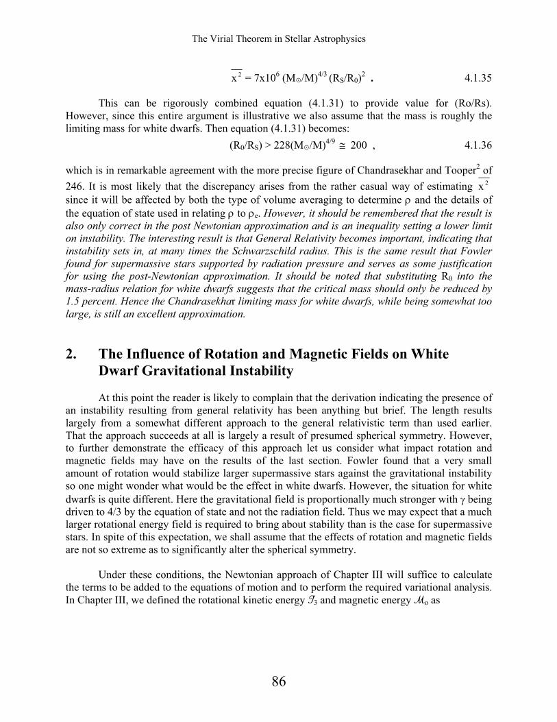
2x = 7x106 (M⊙/M)4/3 (RS/R0)2 . 4.1.35 This can be rigorously combined equation (4.1.31) to provide value for (Ro/Rs). However, since this entire argument is illustrative we also assume that the mass is roughly the limiting mass for white dwarfs. Then equation (4.1.31) becomes:

(R0/RS) > 228(M⊙/M)4/9 ≅ 200 , 4.1.36 which is in remarkable agreement with the more precise figure of Chandrasekhar and Tooper2 of 246. It is most likely that the discrepancy arises from the rather casual way of estimating 2x since it will be affected by both the type of volume averaging to determine ρ and the details of the equation of state used in relating ρ to ρe. However, it should be remembered that the result is also only correct in the post Newtonian approximation and is an inequality setting a lower limit on instability. The interesting result is that General Relativity becomes important, indicating that instability sets in, at many times the Schwarzschild radius. This is the same result that Fowler found for supermassive stars supported by radiation pressure and serves as some justification for using the post-Newtonian approximation. It should be noted that substituting R0 into the mass-radius relation for white dwarfs suggests that the critical mass should only be reduced by 1.5 percent. Hence the Chandrasekhar limiting mass for white dwarfs, while being somewhat too large, is still an excellent approximation. 2. The Influence of Rotation and Magnetic Fields on White Dwarf Gravitational Instability At this point the reader is likely to complain that the derivation indicating the presence of an instability resulting from general relativity has been anything but brief. The length results largely from a somewhat different approach to the general relativistic term than used earlier. That the approach succeeds at all is largely a result of presumed spherical symmetry. However, to further demonstrate the efficacy of this approach let us consider what impact rotation and magnetic fields may have on the results of the last section. Fowler found that a very small amount of rotation would stabilize larger supermassive stars against the gravitational instability so one might wonder what would be the effect in white dwarfs. However, the situation for white dwarfs is quite different. Here the gravitational field is proportionally much stronger with γ being driven to 4/3 by the equation of state and not the radiation field. Thus we may expect that a much larger rotational energy field is required to bring about stability than is the case for supermassive stars. In spite of this expectation, we shall assume that the effects of rotation and magnetic fields are not so extreme as to significantly alter the spherical symmetry. Under these conditions, the Newtonian approach of Chapter III will suffice to calculate the terms to be added to the equations of motion and to perform the required variational analysis. In Chapter III, we defined the rotational kinetic energy T3 and magnetic energy Mo as

86


π=

ω=

∫

∫

V

2

0 21

3

dV8H

d

M

LTL

, 4.2.1

which have variations

ξ−=δξ−=δMMTT )0(2 33 . 4.2.2

Adding this to the variational form of Lagrange's identity in section 1 [equation (4.1.21)], we get

( ) 1131r2

2

21 21213I

dtd

Ωδ−δ>−Γ<+δ+δ+Ωδδ>−Γ<=δ UMT-U 1 . 4.2.3

. Now the condition on the variation of the total energy becomes

1130E Ωδ−δ+δ+δ+Ωδ−δ==δ UMTU , 4.2.4 which enables us to re-write 4.2.3 as

( ) )(3512(43Idtd

1111r2

2

21 Ωδ−δ>Γ−<+δ>−Γ<−δ−δ>−Γ=<δ 31 TUM)U . 4.2.5

Substituting in the values for the variations we get an expression analogous to equation (4.1.24)

)]0([53214)(43I 31111001r2 TUM −Ω>−Γ<+>−Γ<−−Ω>−Γ=<σ y . 4.2.6

These expressions differ from those in Chapter III only because the gravitational potential energy is taken here to be positive. In order for us to proceed further it will be necessary to normalize both the rotational energy and magnetic field by something. Let us consider the case for ridged rotation so that

II 231

z2

21

3 ω=ω=T . 4.2.7 Here we are ignoring the relativistic corrections to I and take I = αMR2. In addition, let us normalize the angular velocity ω by the critical value for a Roche model. Then

=

=ω 2

00

22

30

22

cRGM2

R27cw4

R27GM8w . 4.2.8

87


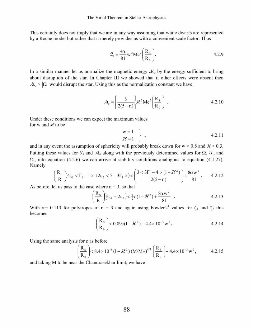
This certainly does not imply that we are in any way assuming that white dwarfs are represented by a Roche model but rather that it merely provides us with a convenient scale factor. Thus

α=

0

S22

RR

Mcw814

3T . 4.2.9

In a similar manner let us normalize the magnetic energy Mo by the energy sufficient to bring about disruption of the star. In Chapter III we showed that if other effects were absent then Mo > Ω would disrupt the star. Using this as the normalization constant we have

−

=0

S220 R

RMc

)n5(23 HM . 4.2.10

Under these conditions we can expect the maximum values for w and H to be

==

11w

H , 4.2.11

and in any event the assumption of sphericity will probably break down for w > 0.8 and H > 0.3. Putting these values for T3 and Mo along with the previously determined values for Ω, Ul, and Ωl, into equation (4.2.6) we can arrive at stability conditions analogous to equation (4.1.27). Namely

( )81w8

)n5(2)1(433

35214RR 22

11211

S α+

−

−>−Γ<<>Γ−<ς+>−Γ<ς

H . 4.2.12

As before, let us pass to the case where n = 3, so that

( )81w8)1(2

RR 2

229

2134S α

+−ε<ς+ς

H . 4.2.13

With α= 0.113 for polytropes of n = 3 and again using Fowler's4 values for ζ1 and ζ2 this becomes

232

0

S w104.4)1(89.0RR −×+−ε<

H . 4.2.14

Using the same analysis for ε as before

)1(104.8RR 28

0

S H−×<

− (M/M⊙)4/3 23

0

S w104.4RR −×+

, 4.2.15

and taking M to be near the Chandrasekhar limit, we have

88


0)1(

103.9)1(

w101.4RR

RR

2

6

2

24

S

0

3

S

0 >−×

−−×

+

−

HH. 4.2.16

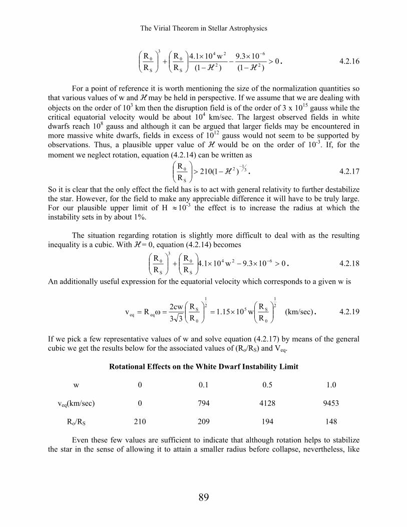
For a point of reference it is worth mentioning the size of the normalization quantities so that various values of w and H may be held in perspective. If we assume that we are dealing with objects on the order of 103 km then the disruption field is of the order of 3 x 1015 gauss while the critical equatorial velocity would be about 104 km/sec. The largest observed fields in white dwarfs reach 108 gauss and although it can be argued that larger fields may be encountered in more massive white dwarfs, fields in excess of 1012 gauss would not seem to be supported by observations. Thus, a plausible upper value of H would be on the order of 10-3. If, for the moment we neglect rotation, equation (4.2.14) can be written as

312

S

0 )1(210RR −

−>

H . 4.2.17

So it is clear that the only effect the field has is to act with general relativity to further destabilize the star. However, for the field to make any appreciable difference it will have to be truly large. For our plausible upper limit of H ≈10-3 the effect is to increase the radius at which the instability sets in by about 1%. The situation regarding rotation is slightly more difficult to deal with as the resulting inequality is a cubic. With H = 0, equation (4.2.14) becomes

0103.9w101.4RR

RR 624

S

0

3

S

0 >×−×

+

− . 4.2.18

An additionally useful expression for the equatorial velocity which corresponds to a given w is

(km/sec)RR

w1015.1RR

33cw2Rv

21

0

S521

0

Seqeq

×=

=ω= . 4.2.19

If we pick a few representative values of w and solve equation (4.2.17) by means of the general cubic we get the results below for the associated values of (Ro/RS) and Veq.

Rotational Effects on the White Dwarf Instability Limit

w

0 0.1 0.5 1.0

veq(km/sec)

0 794 4128 9453

Ro/RS 210 209 194 148

Even these few values are sufficient to indicate that although rotation helps to stabilize the star in the sense of allowing it to attain a smaller radius before collapse, nevertheless, like

89


magnetic fields, the effect is small. One may choose to object to the assumption of rigid rotation as being too conservative. However, it is clear from the development that for either rotation or magnetic fields to really play an important role the total energy stored by either mechanism must approach that in the gravitational field. In order to do this with differential rotation, the differential velocity field would have to be alarmingly high. It seems likely that the resulting shear would produce significant dynamical instabilities. Thus, we have seen that neither magnetic fields nor rotation can significantly alter the fact that a white dwarf will become unstable at or about 1000 km. Classically, the star reaches this point when it is within, but less than, a few percent of the Chandrasekhar limiting mass. So it is not the limiting mass resulting from the change in the equation of state that keeps us from observing more massive white dwarfs. Rather it is the presence of general relativistic instability that destroys any more massive objects. It is quite simple to dismiss this argument as 'nit-picking' as the mass at which the instability occurs is nearly identical to the Chandrasekhar limiting mass. However, when one tries to generalize the results of one problem to another, it is conceptual errors such as this that may lead to much more serious errors in the generalization. As we shall see in the next section, this is indeed the case with neutron stars. 3. Stability of Neutron Stars A second class of objects whose existence became well established during the 1960's is the neutron stars. It is a commonly held misconception that a neutron star is nothing more than a somewhat collapsed white dwarf, since the masses are thought to be similar. In reality the ratios of typical white dwarf radii to neutron stars is suspected to be nearly 1000 which is just about the ratio of the sun's radius to that of a typical white dwarf. A similar misconception relates to the notion of the neutron star’s limiting mass. It is popular to suggest that since the mass limit in white dwarfs arises as a result of the change in the equation of state so a similar change in the equation of state for a neutron star yields a limiting mass for these objects. It is true that a limiting mass exists for neutron stars but this limit does not primarily arise from a change in the equation of state. Let us consider a very simple argument to dramatize this point. The equation of the state change that results in the Chandrasekhar limit occurs because the electrons achieve relativistic velocities. If this were to happen in neutron stars, the configuration would still have to satisfy the virial theorem. For the moment let us ignore the effects of general relativity and just consider the special relativistic virial theorem as we derived in Chapter II [equation (2.3. 9)].

90


∫ γτ++Ω=V

2r

2

21 dV)/(T

dtId , 4.3.1

where now γ = (1- v2/c2)-1/2. As the neutrons become relativistic γ -1 → 0 and T = αMc2 where α >>1. We may write the gravitational potential energy as

η−=η−=Ω

0

S2

0

2

RR

2Mc

RGM . 4.3.2

The variational form of the virial theorem will require that T + Ω < 0 , 4.3.3

so that Mc2[α−(η/2)(RS/R0)] < 0 , 4.3.4

or (R0/RS) > η/2α . Since η is of the order of unity and α >> 1, this would require that the object have a radius less than the Schwarzschild radius in order to be stable against radial pulsations. This is really equivalent to invoking Jacobi's stability condition on the total energy. This simplistic argument can be criticized on the grounds that it ignores general relativity which can be viewed as increasing the efficiency of gravity. Perhaps the "increased gravity" would help stabilize the star against the rapidly increasing internal energy. This is indeed the case for awhile. However, based on the analysis in section 1, as the value of Γ approaches 4/3 the same type of instability which brought about the collapse of the white dwarfs will occur in the neutron stars. The exact value of Ro/RS for which this happens will depend on the exact nature of the equation of state as well as details of model construction. However, since the general relativistic correction terms will be much larger than in the case of white dwarfs, we should expect the value of Γ to depart farther from the relativistic limit of 4/3 than before. That this is indeed the case is clearly shown by Tooper7 in considering the general properties of relativistic adiabatic fluid spheres. He concludes that the instability always occurs before the gas has become relativistic at high pressures. Unfortunately we cannot quantitatively apply the results of Section 1 since the way in which Γ approaches 4/3 (more properly the way in which Γ departs from 5/3) depends in detail on the equation of state. However, we may derive some feeling for the way in which the instability sets in by assuming the compression has driven the value of Γ down from 5/3 to 3/2 (i.e., just half way to its relativistic value. Substitution of Γ = 3/2 in equation (4.1.27) and using Fowler’s4 values of ζl and ζ2 for a polytrope of index 2 gives a stability limit of

3.4RR

S

0 >

. 4.3.5

Thus Ro for a neutron star would have to be greater than about 12 km. Since typical model radii are of the order of 10 km, 3/2 is probably a representative value of Γ, yet it is still far from the relativistic value of 4/3. This argument further emphasizes the fact that it is the general

91


relativistic instability which places an upper limit on the size of the configuration, not the equation of state becoming relativistic. The discussion in section 2 would lead us to believe that neither rotation nor magnetic fields can seriously modify the onset of the general relativistic instability. This can be made somewhat quantitative by evaluating equation (4.2.10) for a polytrope of index n = 2. However, in order to do this, we must re-evaluate the moment of inertia weighting factor a. A crude estimate here will suffice since we are neglecting an increase of perhaps a factor of 2 due to

general relativistic terms. One can show by integrating 4 by parts in Emden polytropic

variables that ∫ ρπ

R

0

2 drr

ξθ

ξ

ξξθξ

+=α

ξ

ξ

∫

1

1

dd

d6

121

021 , 4.3.6

which for n = 2 very approximately gives α = 0.345. Substitution into 4.2.13 then yields

222

0

S w102.3)1(234.0RR −×+−<

H . 4.3.7

The effects of magnetic fields and rotation are qualitatively the same for neutron stars as for white dwarfs. However, as Ro is only a few times the Schwarzschild radius, the normalizing fields and rotational velocities are truly immense. For a neutron star with a 10 km radius the magnetic field corresponding to H = 1 in of the order of 1018 gauss while the rotational velocity corresponding to w = 1 would be about 10% the velocity of light. These values vastly exceed those for the most extreme pulsar. Thus, barring modification to the equation of state resulting from these effects, they can largely be ignored in investigating neutron star stability. This result is exactly in accord with what one might have expected on the basis of the white dwarf analysis. We began this discussion by indicating that the analysis would be very simplistic and yet we have attained some very useful qualitative results. Since the mass-radius law for any degenerate equation of state (excepting small technical wiggles) will provide for stars whose radius decreases with increasing mass, we can guarantee that the resulting decrease in Γ will give rise to an unstable configuration at a few Schwarzschild radii. Thus, there will exist an upper limit to the mass allowable for a neutron star. The origin of this limit is conceptually identical to that for white dwarfs. Furthermore, as for white dwarfs, this limit can be modified by the presence of magnetic fields and rotation only for the most extreme values of each. One may argue that in discussing effects of general relativity we have included terms of O (1/c2) and that higher order effects may be important. While this is true regarding such items as gravitational radiation, none of these terms should be important unless the configuration becomes smaller than several Schwarzschild radii.

92


Even then, they are unlikely to affect the qualitative behavior of the results. Very little has been said about the large volume of work relating to the equation of state for neutron degenerate matter. This is most certainly not to deny its existence, just its relevance. One of the strong points of this approach is that insight can be gained into the global behavior of the object without undue concern regarding the microphysics. This type of analysis is a probe intended to ascertain what effects are important in the construction of a detailed model and what may be safely ignored. It cannot hope to provide the information of a detailed structural model but only point the way toward successful model construction. 4. Additional Topics and Final Thoughts It would be possible and perhaps even tempting to continue demonstrating the efficacy of the virial theorem in stellar astrophysics. However, attempting to exhaust the possible applications of the virial theorem is like trying to exhaust the applicability of the conservation of momentum. I would be remiss if I did not indicate at least some other possible areas in which the virial theorem can lend insight. In Chapter III, section 4 we discussed the variational effect of the surface terms resulting from the application of the divergence theorem. These terms are generally neglected and for good reason. In most cases the bounding surface can be chosen so as to include the entire configuration. In instances where this is not the case, such as with magnetic fields, the term is still generally negligible. If one considers the form of the surface terms given by equation (2.5.19) (Chapter II), compared to the volume contribution [i.e. equation (2.5.18)], the ratio of the scalar value is

><=

•=ℵ∫

∫PP

PdV

dP0

V

S0 Sr

, 4.4.1

where <P> is the average value of the internal pressure. Since, in any equilibrium configuration the pressure must be a monotone increasing function as one moves into the configuration, ℵ< 1. In general it is very much less than one. However, in the case where γ→ 4/3 the variational contribution of the surface pressure approaches ∫ • Sr dP3 0 , while the internal pressure and Newtonian gravity contributions vanish. Such terms are then available to combine with the effects of general relativity. Since they are of the same sign as the general relativistic terms the surface terms will only serve to increase the instability of the entire configuration. This results in an increase of the radius at which white dwarfs become unstable. Thus, the accretion of matter onto the surface of such objects may cause them to collapse sooner than one might otherwise expect.

93


Since magnetic fields also are usually assumed to increase inward, the influence of magnetic surface terms will be similar to that of a non-zero surface pressure. Like the surface pressure terms, they will in general be small compared to the internal contributions. Only in case of a system with an effective γ approaching 4/3 could these small terms be expected to exert a trigger effect on the resulting configuration. There is one instance in which the use of the surface terms can be significant. One of the most attractive aspects of this entire approach is that it can deal with the properties of an entire system. Indeed the spatial moments are taken in order to achieve that result. However it is interesting to consider the effects of applying the virial theorem to a sub-volume of a larger configuration. Clearly, as one shrinks the volume to zero he recovers the equations of motion themselves multiplied by the local positional coordinate. If one considers a case intermediate to these limits and investigates the stability of a sub-volume which could include the surface of the star, it would be possible to analyze the outer layer for instabilities which might not be globally apparent. It is true that a local stability criterion would be sufficient to locate such instabilities but one could not be sure how the instabilities would propagate without carrying out a large structural analysis. This latter effect can be avoided by utilizing a sub-global form of the virial theorem. Under these conditions one might expect the surface terms to be the dominant terms of the resulting expression. In discussing some of the more bizarre and contemporary aspects of stellar structure it is easy to overlook the role played by the virial theorem in the development of the classical theory of stellar structure. It is the virial theorem which provides the theoretical basis for the definition of the Kelvin-Helmholtz contraction time. This is just the time required for a star to radiate away the available gravitational potential energy at its present luminosity. It is the virial theorem which essentially tells how much of the gravitational energy is available. Thus if the contraction liberating the potential energy is uniform and d2I/dt2 is zero then the total kinetic energy always must be

T = -1/2 Ω . 4.4.2 This makes the other half of the gravitational energy available to be radiated away. The Kelvin-Helmholtz contraction time for poly tropes is thus

n5105.4

RL)n5(2GM3 72

−×

≅−

=T (M/M⊙)2(R⊙L⊙/RL) (years). 4.4.3

Reasoning that this provided an upper limit to the age of the sun Lord Kelvin challenged the Darwinian theory of evolution on the sound ground that 23 million years (i.e. KHT for a polytrope with an internal density distribution of n=3)8 was not long enough to allow for the evolutionary development of the great diversity of life on the planet. The reasoning was flawless, only the initial assumption that the sun derived its energy from gravitational contraction which was plausible at the time, failed to withstand the development of stellar astrophysics.

94


Another aspect of classical stellar evolution theory is clarified by application of the virial theorem. All basic courses in astronomy describe post-main sequence evolution by pointing out that the contraction of the core is accompanied by an expansion of the outer envelope. Most students find it baffling as to why this should happen and are usually supplied with unsatisfactory answers such as "it's obvious" or "it's the result of detailed model calculations" which freely translated means "the computer tells me it is so." However, if the virial theorem is invoked, then once again any internal re-arrangement of material that fails to produce sizable accelerative changes in the moment of inertia will require that

2T+Ω = 2E-Ω = 0 . 4.4.4 Since the only way that the star can change its total energy E without outside intervention is by radiating it away to space, any internal changes in the mass distribution which take place on a time scale less than the Kelvin Helmholtz contraction time will have to keep the total energy and hence the gravitational potential energy constant. Now

Ω = -αM2/R . 4.4.5 where α is a measure of the central condensation of the object, so, as the core contracts and α increases, R will have to increase in order to keep Ω constant. In general the evolutionary changes in a star do take place on a time scale rather less than the contraction time and thus we would expect a general expansion of the outer layer to accompany the contraction of the core. The microphysics which couples the core contraction to the envelope expansion is indeed difficult and requires a great deal of computation to describe it in detail. However the mass distribution of the star places constraints on the overall shape it may take on during rapid evolution processes. It is in the understanding of such global problems that the virial theorem is particularly useful. I have attempted throughout this book to emphasize that global properties are the very essence of the virial theorem. The centrality of taking spatial moments of the equations of motion to the entire development of the theorem demonstrates this with more clarity than any other aspect. Although this global structure provides certain problems when the development is applied to continuum mechanics nothing is encountered within the framework of Newtonian mechanics which is insurmountable. Only within the context of general relativity may there lie fundamental problems with the definition of spatial moments. Even here the first order theory approximation to general relativity yields an unambiguous form of the virial theorem for spherical objects. In addition, certain specific time independent or at least slowly varying cases of the non-approximated equations also yield unique results. Thus one can realistically hope that a general formulation of the virial theorem can be made although one must expect that the interpretation of the resultant space-time moments will not be intuitively obvious. The rather recent development of the virial theorem provides us with a dramatic example of the fact that theories do not develop in an intellectual vacuum. Rather they are pushed and shoved into shape by the passage of the time. Thus we have seen the virial theorem born in an effort to clarify thermodynamics and arising in parallel form in classical dynamics. However the similarity did not become apparent until the implications of the ergodic theorem inspired by

95


statistical mechanics were understood. Although sparsely used by the early investigators of stellar structure, the virial theorem did not really attract attention until 1945 when the global analysis aspect provided a simple way to begin to understand stellar pulsation. The attendant stability analysis implied by this approach became the main motivation for further development of the tensor and relativistic forms and provides the primary area of activity today. Only recently has the similarity of virial theorem development to that of other conservation laws been clearly expounded. Recent criticism of some work utilizing the virial theorem, incorrectly attacks the theorem itself as opposed to analyzing the application of the theorem and the attendant assumptions. This is equivalent to attacking a conservation law and serves no useful purpose. Indeed it may, by rhetorical intimidation, turn some less sophisticated investigators aside from consideration of the theorem in their own problems. This would be a most unfortunate result as by now even the most skeptical reader must be impressed by the power of the virial theorem to provide insight into problems of great complexity. Although there is a trade-off in that a complete dynamical description of the system is not obtainable, certain general aspects of the system are analyzable. Even though some might claim a little knowledge to be a dangerous thing, I prefer to believe that a little knowledge is better than none at all. Thus, the perceptive student of science will utilize the virial theorem to provide a 'first look' at problems to see which are of interest. Used well this first look will not be the last. Through the course of this book we have examined the origin of the virial theorem, noted its development and applicability to a wide range of astrophysical problems, and it is irresistible to contemplate briefly its future growth. In my youth the course of future events always seemed depressingly clear but turned out to be generally wrong. Now, in spite of a better time base on which to peer forward, the new future seems at best "seen through a glass darkly", and I am mindful that astronomers have not had an exemplary record as predictors of future events†. Nevertheless, there may be one or two areas of growth for the virial theorem on which we can count with some certainty. Immediate problems which seem ideally suited to the application of the virial theorem certainly include exploration into the nature of the energy source in QSO's. Perhaps one will finally observe that the gravitational energy of assembly of a galaxy or its components is of the same order as the estimated energy liberated by a QSO during its lifetime. The virial theorem implies that half of this energy may be radiated away. Thus, it would appear that one need not look for the source of such energy but rather be concerned with the details of the "generator". †___________________________ It is said that the great American astronomer, Simon Newcomb "proved" that heavier than air flight was impossible and that after the Wright Brothers flew, it was rumored that he maintained it would never be practical as no more than two people could be carried by such means.

96


Perhaps future development will consider applications of the virial theorem as represented by Lagrange's identity. To date the virial theorem has been applied to systems in or near equilibrium. It is worth remembering that perhaps the most important aspect of the theorem is that it is a global theorem. Thus systems in a state of rapid dynamic change are still subject to its time dependent form. In the mid twentieth century, as a consequence of discovering that the universe is not a quiet place, theoreticians became greatly excited about the properties of objects undergoing unrestrained gravitational collapse. It is logical to suppose that sooner or later they will become interested in the effects of such a collapse upon fields other than gravitation (i.e. magnetic or rotational), that may be present. The virial theorem provides a clear statement on how the energy in such a system will be shifted from one form to another as soon as one has determined d2I/dt2. Future investigation in this area may be relevant to phenomena ranging from novae to quasars. Perhaps the most exciting and at the same time least clear and speculative development in which the virial theorem may play a role involves its relationship to general relativity. This is a time of great activity and anticipatory excitement in fundamental physics and general relativity in particular. Perhaps through the efforts of Stephan Hawking and others, and as Denis Sciama has noted, we are on the brink of the unification of general relativity, quantum mechanics, and thermodynamics. Thermodynamics is the handmaiden of statistical mechanics and it is here through the application of the ergodic theorem that the virial theorem may play its most important future role. You may remember that in Chapter II, difficulty in the interpretation of moments taken over space-time frustrated a general development of the virial theorem in general relativity and it was necessary to invoke first order approximations to the relativistic field equations. In addition the ergodic theorem seems inexorably tied to the nature of reversible and irreversible processes. The advances in relating general relativity to thermodynamics bring these areas and theorems into direct conceptual confrontation and may perhaps provide the foundations for the proper understanding of time itself.

97


Notes to Chapter 4 4.1 The last integral can be integrated by parts so that

∫∫∫

∫∫

∫∫ ∫

π+

π−

π+

ρ=

+

π+

π−

ρ=

π−

π−

π=

ρπ

R

0

R

0 22

R

02

V22

22

R

02

R

02

V22

22

R

0V

R

0 2

2R

02

2

2

2

drdrdP)r(m

cG8dr

drdP)r(m

cG8)r(P)r(m

cG8dV

cr)r(mG

drdrdPP)r(m

cG8Pr)r(m

cG8dV

cr)r(mG

rdrc

P)r(Gm8drdrdP

c)r(Gmr4

c)r(mPrG4dV

cPrG4

N4.1.1

The third term vanishes since m(0) = 0 and P(R) = 0, the last two integrals cancel so that

dVcr

)r(mGdVcPrG4

V22

22

V2

2

∫∫ρ

=ρπ . N4.1.2

4.2 Start1ng w1th the polytropic equation of state

p=Kργ . N4.2.1 It is not hard to convince yourself that

ρρ

=ρ

=γddP

PndnPd . N4.2.2

This can be reduced to a sing1e parameter by considering Chandrasekhar's parametric equation of state for a nearly re1ativistic degenerate gas6

3Bx),x(AfP =ρ= , N4.2.3 where f(x) = x(2x2-3) (x2 +1) + 3 Sinh-1 (x). The limit of the hyperbolic sine is:

[ ] x2ln)x(sinhx

Lim 1 =∞→

− . N4.2.4

Now consider the behavior of f(x) as x → ∞ .

−≅

+⋅⋅⋅+−−+=⋅+⋅⋅++−−≅ −−

)x2(xf(x)or

xx3xx2)xx)(3x)(3x2(x)x(f

24

1232241

2122

. N4.2.5

98


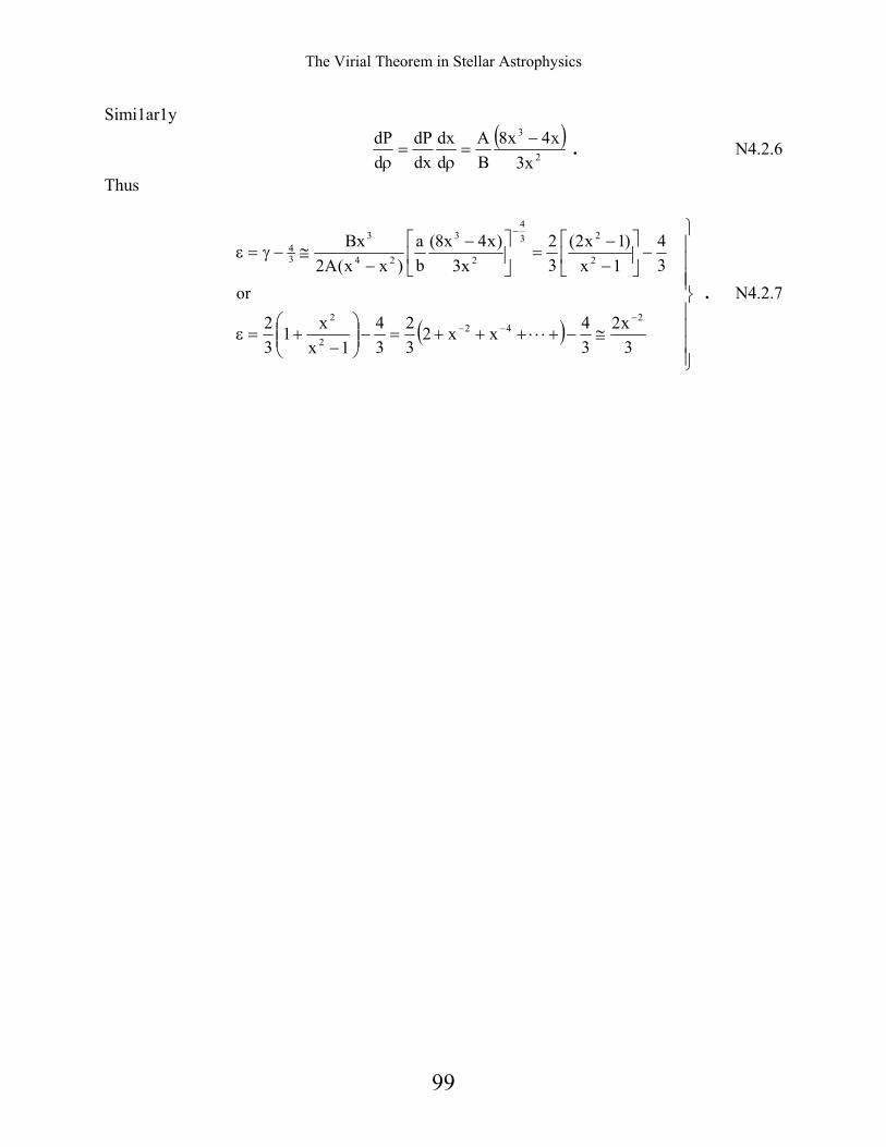
Simi1ar1y ( )

2

3

x3x4x8

BA

ddx

dxdP

ddP −

=ρ

=ρ

. N4.2.6

Thus

( )

≅−+⋅⋅⋅+++=−

−

+=ε

−

−−

=

−−

≅−γ=ε

−−−

−

3x2

34xx2

32

34

1xx1

32

or34

1x)1x2(

32

x3)x4x8(

ba

)xx(A2Bx

242

2

2

2

234

2

3

24

3

34

. N4.2.7

99


References 1 Thorne, K. S. (1972), Stellar Evolution, (ed. Hang-Yee Chin and Amador Muriel)

M.I.T. Press, Cambridge, Mass. p. 616. 2 Chandrasekhar, S. and Tooper, R. F. (1964), Ap. J. 139, p. 1396. 3 Meltzer, D. W. and Thorne, K. S. (1966), Ap. J. 145, p. 514. 4 Fowler, W. A. (1966), Ap. J. 144, p. 180. 5 Faulkner, J. and Gribbin, J. R. (1966), Nature, Vol. 218, p. 734-7. 6 Chandrasekhar, S. (1957), An Introduction to the Study of Stellar Structure, Dover Pub., pp. 360-361. 7 Tooper, R. F. (1965), Ap. J. 142, p. 1541. 8. Chandrasekhar, S. (1957), An Introduction to the Study of Stellar Structure, Dover Pub., pp. 454-455. 9. Fricke, K.J. (1973). Ap. J. 183, pp. 941-958.

100


101

IV Some Applications of the Virial Theoremads.harvard.edu/books/1978vtsa.book/Chapt4.pdf · IV Some...

Documents

Transcript of IV Some Applications of the Virial Theoremads.harvard.edu/books/1978vtsa.book/Chapt4.pdf · IV Some...