Item Response Theory Models for Forced-Choice Questionnaires
171
Item Response Theory Models for Forced-Choice Questionnaires by Daniel Morillo A dissertation submitted to the Faculty of Psychology in Universidad Autónoma de Madrid in partial fulfillment of the requirements for the degree of Philosophy Doctor in Clinical and Health Psychology Supervised by: Dr. Francisco J. Abad, and Dr. Iwin M. Leenen Mentored by: Dr. Vicente Ponsoda July 2018 Madrid, Spain
Transcript of Item Response Theory Models for Forced-Choice Questionnaires

Item Response Theory Models for Forced-Choice Questionnaires
by
Daniel Morillo
A dissertation submitted
to the Faculty of Psychology
in Universidad Autónoma de Madrid
in partial fulfillment of the requirements for the degree of
Philosophy Doctor in Clinical and Health Psychology
Supervised by: Dr. Francisco J. Abad, and Dr. Iwin M. Leenen
Mentored by: Dr. Vicente Ponsoda
July 2018
Madrid, Spain

i
Acknowledgements
There is many people I am in debt with respect to this dissertation. I feel that I would
not have been able to accomplish this if it were not for the support of those that have provided
me with their guidance, wisdom, and over all, affection. My supervisors have done an
exceptional job helping me get to this point. To Iwin Leenen (Universidad Nacional Autónoma
de México), Paco Abad, and Vicente Ponsoda (both from Universidad Autónoma de Madrid),
I owe my most sincere gratitude. The rest of the people in our team have provided with
invaluable support, ideas, and a critical points of view: Pedro Hontangas (Universidad de
Valencia), Rodrigo Kreitchmann (Universidad Autónoma de Madrid), and Jimmy de la Torre
(University of Hong Kong), many thanks to you. The faculty members in the School of
Psychology, Universidad Autónoma de Madrid, and especially in the department of Social
Psychology and Methodology have often been a source of intellectual challenges. I am
especially in debt with Julio Olea, professor of psychometry in the Chair of Psychometric
Models and Applications, whom along with Vicente put their trust in me in the beginnings of
my research career, granting me the internship that allowed me to start my Ph.D. studies later
on. The Ph.D. candidate research assisstants have been an incredible support throughout these
years. I feel so proud of having been part of such a collective, which came to be a reference
model for other predoctoral collectives in our university. Some professors and researchers
have given me the opportunity to make my first steps into the world of research, or have given
me the opportunity to collaborate with their projects. To them I owe my most sincere thanks
as well, especially, Mª Ángeles Quiroga (Universidad Complutense de Madrid), Roberto
Colom (Universidad Autónoma de Madrid), and Belén López (Liverpool Hope University).
I can feel fortunate to have had the chance to “step out” and enrich my views in many
ways. I am especially grateful with Anna Brown (Univerity of Kent in Canterbury) and Mark
Hansen (CRESST, UCLA), who hosted me in Canterbury and L.A., respectively, and gave me

ii
the opportunity to learn and develop my skills. Many people have given me support, advice,
or even have made me challenge my points of view, giving me reasons to keep up. I would
like to thank Minjeong Jeon (UCLA), Peter Bentler (UCLA), Juan Ramón Barrada
(Universidad de Zaragoza), and Albert Maydeu (University of South Carolina) for this. Also,
the people in the Junior Researcher Programme have given me a great opportunity to expand
my skills and gain valuable experience. Among them I’d like to thank especially the
supervisors, and the Junior Researchers in my team: Thanks so much to you all!
The last part is the most difficult one, for I fear I may forget someone. Friends and
relatives are the most important support one can have, and it’s not different in my case. For
these years, they have been a constant source of help and affection. Even when they have had
to assume I would be unavailable for most of them: Manu, Javi “Fido”, Belén, Raúl “Moe”,
Jorge “Yorch”, Raquel, Clara, Davide, Carol, and many more from the “Aluche” crew; those
that have always been there, even in spite of their family duties: Javi, Dani (a constant source
of “food for thought”), Giorgio, David “Palas”, Ruth, Olga and Pablo, Olga, Ana, and their
families, my greatest thanks go to all of them; to the ones who started with me the journey of
understanding those weird little creatures called “humans”, Gabi, Laura P., Kristti, Borja,
María, Mari “Angus”, “El mago” Tony, Laura C., Alvarito, Bárbara “Baco”, Nilda, Lara,
Andrés, Dani “Lutiako”, and many, many more… I can’t say how much I enjoyed that journey
with you all! Carol, Natxo, and all the people in Alusamen, I’m so grateful for having had the
opportunity of learning from you and sharing so many good moments. My family who have
given me the most trust, support, and affection, have a special place; I want to especially thank
my mother, my sister Marta, and my cousin Juan. Finally (last but not least), one person must
have a special place, for she has endured the ups and downs of this dissertation as much as
myself; to Fátima, my most special thanks and all my love.

iii
Para Fátima.

v
Table of contents
Abstract ...................................................................................................................................... 1
Resumen ..................................................................................................................................... 3
Chapter 1: General introduction................................................................................................. 5
1.1. The development of the forced-choice format ............................................................ 6
1.2. Understanding the forced-choice response format ...................................................... 7
1.2.1. The validity of forced-choice questionnaire measures ......................................... 9
1.2.1.1. The forced-choice format as a means for controlling response biases ........ 10
1.2.1.2. The notion of ipsativity and its statistical approach .................................... 15
1.2.1.3. Concluding remarks about the validity of FC ipsative measures ................ 19
1.3. The application of item response theory to multidimensional forced-choice data ... 20
1.3.1. Early antecedents ................................................................................................ 20
1.3.2. Foundations of IRT models for multidimensional forced-choice data ............... 22
1.3.3. The emergence of IRT models for multidimensional forced-choice data .......... 25
1.3.4. State-of-the-art IRT models ................................................................................ 26
1.4. Motivation of this dissertation................................................................................... 27
Study 1: A Dominance Variant under the Multi-Unidimensional Pairwise-Preference
Framework: Model Formulation and Markov Chain Monte Carlo Estimation ................ 28
Study 2: Assessing and reducing psychometric issues in the design of multidimensional
forced-choice questionnaires for personnel selection ....................................................... 29
Study 3: Testing the invariance assumption of the MUPP-2PL model ............................ 29
Chapter 2: A Dominance Variant under the Multi-Unidimensional Pairwise-Preference
Framework: Model Formulation and Markov Chain Monte Carlo Estimation ....................... 31
Abstract ................................................................................................................................ 31
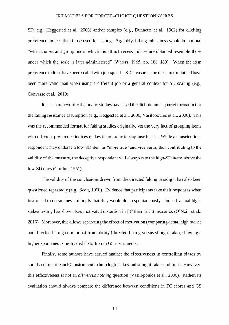
2.1. The MUPP-2PL Model ............................................................................................. 36
2.1.1. Relationships of the MUPP-2PL to other models .............................................. 38
2.1.1.1. Relationship with the Multidimensional Compensatory Logistic Model .... 38
2.1.1.2. Relationship with the TIRT model .............................................................. 38
2.2. Bayesian Estimation of the MUPP-2PL .................................................................... 39
2.2.1. Identification of latent trait and item parameters ................................................ 40
2.3. Simulation Study ....................................................................................................... 41
2.3.1. Design and data generation process .................................................................... 41
2.3.2. MCMC analysis .................................................................................................. 42
2.3.3. Goodness-of-recovery summary statistics .......................................................... 42
2.3.4. Results ................................................................................................................ 43
2.3.4.1. Correlation parameters (𝚺𝜃) ........................................................................ 46
2.3.4.2. Latent trait parameters (𝛉) ........................................................................... 46
2.3.4.3. Scale parameters (𝐚) .................................................................................... 46
2.3.4.4. Intercept parameters (𝐝) .............................................................................. 47

vi
2.3.5. Comparison with the TIRT estimation ............................................................... 47
2.4. Empirical Study ......................................................................................................... 49
2.5. Discussion ................................................................................................................. 51
References ............................................................................................................................ 55
Chapter 3: Assessing and Reducing Psychometric Issues in the Design of Multidimensional
Forced-Choice Questionnaires for Personnel Selection .......................................................... 61
Abstract ................................................................................................................................ 61
3.1. MUPP-2PL for forced-choice blocks ........................................................................ 65
3.1.1. Graphical representation of MUPP-2PL blocks ................................................. 65
3.1.1.1. Multidimensional block location ................................................................. 66
3.1.1.2. Multidimensional block scale ...................................................................... 67
3.1.1.3. Block measurement direction ...................................................................... 68
3.1.1.4. Vector representation ................................................................................... 68
3.1.2. Multivariate information function of a FCQ ...................................................... 70
3.2. Binary forced-choice questionnaires for controlling social desirability ................... 71
3.3. Empirical underidentification of the MUPP-2PL model in a DBP FCQ .................. 73
Theorem 1 ......................................................................................................................... 75
Theorem 2 ......................................................................................................................... 78
3.4. Quality indices for assessing a FCQ dimensional sensitivity ................................... 79
3.4.1. Least Singular Value .......................................................................................... 81
3.4.2. Least Eigenvalue ................................................................................................. 82
3.5. Simulation Study 1 .................................................................................................... 83
3.5.1. Design and method ............................................................................................. 84
3.5.1. Results and discussion ........................................................................................ 85
3.6. Simulation Study 2 .................................................................................................... 87
3.6.1. Design and method ............................................................................................. 88
3.6.2. Data analysis ....................................................................................................... 89
3.6.3. Results ................................................................................................................ 90
3.6.3.1. Analysis of Variance ................................................................................... 90
3.6.3.2. Dimensional sensitivity indices ................................................................... 92
3.6.4. Discussion ........................................................................................................... 94
3.7. General discussion..................................................................................................... 95
3.7.1. DBP design of forced-choice questionnaires ...................................................... 95
3.7.2. MUPP-2PL empirical underidentification .......................................................... 96
3.7.3. Dimensional sensitivity indices .......................................................................... 98
3.7.4. Generalization of the results ............................................................................... 99
References .......................................................................................................................... 101
Chapter 4: Testing the invariance assumption of the MUPP-2PL model .............................. 105
Abstract .............................................................................................................................. 105
4.1. A test of the invariance assumption with graded scale items and forced-choice
blocks 110
4.2. Aim of the study ...................................................................................................... 112

vii
4.3. Method .................................................................................................................... 113
4.3.1. Materials ........................................................................................................... 113
4.3.1.1. Instruments. ............................................................................................... 113
4.3.1.2. Participants ................................................................................................ 114
4.3.2. Data analysis ..................................................................................................... 115
4.3.2.1. Estimation of the latent trait models .......................................................... 115
4.3.2.2. Exploration of the violations of the invariance assumption ...................... 117
4.4. Results ..................................................................................................................... 118
4.4.1. Dimensionality assessment of the GS questionnaire ........................................ 118
4.4.2. Tests of the invariance assumption ................................................................... 122
4.4.3. Exploration of the violations of the invariance assumption ............................. 126
4.4.3.1. Scale parameters ........................................................................................ 126
4.4.3.2. Intercept parameters .................................................................................. 127
4.5. Discussion ............................................................................................................... 130
4.6. Conclusions ............................................................................................................. 133
References .......................................................................................................................... 136
Chapter 5: General conclusions ............................................................................................. 141
5.1. Summary of the most relevant findings .................................................................. 142
5.2. Limitations and future research lines ...................................................................... 144
Capítulo 6: Conclusiones generales ....................................................................................... 147
6.1. Resumen de los hallazgos más importantes ............................................................ 148
6.2. Limitaciones y líneas de investigación futuras ....................................................... 151
References .............................................................................................................................. 155
Apprendices: Chapter 2 supplementary materials ................................................................. 167
Appendix A: MUPP-2PL model information function ...................................................... 167
Appendix B: Bayesian Estimation algorithm for the MUPP-2PL model estimation ......... 168
B.1. MCMC sampling scheme ................................................................................. 168
B.1.1. Step 1 (drawing 𝚺𝜃(𝑡)
) ................................................................................. 168
B.1.2. Step 2 (drawing 𝛉(𝑡)). ................................................................................ 169
B.1.3. Step 3 (drawing 𝐚(𝑡)). ................................................................................ 170
B.1.4. Step 4 (drawing 𝐝(𝑡)). ................................................................................ 171
B.2. Initialization of the chains ................................................................................ 171

ix
List of tables
Table 2.1. Mean Goodness-of-Recovery for Each Level of Questionnaire Length, Opposite-
Polarity Block Proportion and Interdimensional Correlation for the MCMC
estimates ................................................................................................................. 44
Table 2.2. Mean Goodness-of-Recovery for Each Level of Questionnaire Length, Opposite-
Polarity Block Proportion and Interdimensional Correlation for the TIRT
estimates ................................................................................................................. 48
Table 2.3. Structure, parameter estimates, correlations and empirical reliabilities (as variance
of the latent trait estimates) of the 30-block forced-choice questionnaire ............. 50
Table 3.1. Marginal means of the statistics and main effect sizes of the three-way ANOVA90
Table 4.1. Distribution of the FC blocks by trait .................................................................. 114
Table 4.2. Diagnostic statistics of the unidimensional GS models, compared to the bi-factor
models .................................................................................................................. 119
Table 4.3. Summary of results of the invariance assumption tests ....................................... 122
Table 4.4. Likelihood ratio test statistics of the constrained models .................................... 125
Table 4.5. Number of non-invariant intercept parameters per item trait and block polarity 127

xi
List of figures
Figure 1.1. The four quadrants of Coombs’ Theory of Data .............................................................. 21
Figure 1.2. Schematic representation of the mapping from a Quadrant I data multidimensional space
(left) to a Quadrant III data unidimensional space (right) ................................................. 23
Figure 1.3. Schematic representation of the mapping from a Quadrant II data multidimensional space
(left) to a Quadrant III data unidimensional space (right) ................................................. 24
Figure 2.1. MUPP-2PL model BCFs of three blocks.......................................................................... 37
Figure 2.2. Plot of the estimates against the true values, across all replications, for the condition
QL = 36, OPBP = 0, IC = .50 ............................................................................................ 45
Figure 2.3. Interaction effect between Opposite-Polarity Block Proportion (OPBP) and Questionnaire
Length (QL) on the Mean Reliability (𝜌��2 ) ........................................................................ 47
Figure 3.1. Graphical representation of three bidimensional (1 to 3) and two unidimensional (4 and 5)
MUPP-2PL blocks, in a bidimensional latent space with correlation 𝜌12 = 0 (left) and
𝜌12 = .5 (right) ................................................................................................................... 69
Figure 3.2. Effect of item directions on the information matrix. ......................................................... 80
Figure 3.3. LSV index value based on the correlation block scale correlation (𝜌𝑎𝑖), the number of
blocks per dimension (𝑛𝑑), and the number of dimensions (𝐷) ........................................ 85
Figure 3.4. LEV value based on the block scale correlation (𝜌𝑎𝑖), the number of blocks per dimension
(𝑛𝑑), the number of dimensions (𝐷), and the correlation sum per latent trait (∑𝜌𝜃) ........ 86
Figure 3.5. Interaction between the effects of the block scale correlation (𝜌𝑎𝑖) the latent trait
correlations (𝜌𝜃) on the mean reliability (𝜌��2 ) ................................................................... 91
Figure 3.6. Scatterplot of the mean reliability (𝜌��2 ) as a function of the LSV (top) and the LEV
(bottom) ............................................................................................................................. 92
Figure 3.7. Scatterplot of the mean correlation bias (∆𝜃��𝑟) as a function of the LSV (top) and the LEV
(bottom) ............................................................................................................................. 93
Figure 4.1. Distribution of the unidimensional scale parameter estimates of the GS items, with respect
of the general factor scale parameters in the bi-factor models ........................................ 119
Figure 4.2. Scatter plot of the GS items scale parameter estimates, on the general factor of the bi-
factor models and on the common factor in the unidimensional models ........................ 120
Figure 4.3. Scatter plot of the GS items scale parameter relative bias, on the bi-factor item
unidimensionality ............................................................................................................ 121
Figure 4.4. Scatter plot of the FC-block scale parameter estimates against the corresponding GS-item
estimates .......................................................................................................................... 123
Figure 4.5. Scatter plot of the block intercept estimates, against their values predicted from the item
intercept parameters ........................................................................................................ 124
Figure 4.6. Deviation of the non-invariant block intercept parameters with respect to their predicted
values from the item intercept parameters ....................................................................... 129

1
Abstract
Multidimensional forced-choice questionnaires are regarded as a means of controlling response
bias. The application of these instruments has been held back historically by the ipsativity of
their scores, which precludes inter-individual comparisons. Item response theory has only been
applied recently, enabling them for normative scaling.
The present dissertation introduces the Multi-Unidimensional Pairwise Preference-2
Parameter Logistic model, an item response model for pairwise forced-choice questionnaires.
It consists of three manuscripts, each with different aims. The first manuscript introduces the
model and proposes a Bayesian estimation procedure for the joint estimation of structural and
incidental parameters. It tests the model estimation under different conditions on a Monte
Carlo study, and on empirical data, and compares the results with a procedure based on
frequentist structural equation modelling.
The second manuscript considers the design of multidimensional forced-choice
instruments for controlling response bias. It delves into the underpinnings of multidimensional
item response theory to demonstrate how this design may lead to an empirical
underidentification under certain conditions, implying a dimensional restriction. The
manuscript proposes indices for assessing the dimensionality, and tests them and the
consequences of the underidentification on simulated data.
The third manuscript tests the invariance assumption of the model, which implies that
the item parameters remain unchanged when paired in forced-choice blocks. It proposes a
methodology for testing the hypotheses, based on the Likelihood ratio of nested models. The
method is then applied to empirical data from forced-choice and graded-scale responses,
showing that the assumption largely holds. The manuscript also explores the conditions that
are likely to induce violations of the invariance assumption, and proposes hypotheses and
methods for testing them.

3
Resumen
Los cuestionarios de elección forzosa multidimensionales son considerados un medio para el
control de los sesgos de respuesta. Históricamente, su aplicación se ha visto obstaculizada por
la ipsatividad de sus puntuaciones, que impide hacer comparaciones entre individuos.
Recientemente, se ha aplicado la teoría de respuesta al ítem en este contexto, la cual permite
obtener medidas normativas.
Esta tesis presenta el modelo Multi-Unidimensional Pairwise Preference-2 Parameter
Logístic para cuestionarios de pares de elección forzosa. Consta de tres manuscritos, cada uno
con objetivos diferentes. El primero presenta el modelo y propone un procedimiento de
estimación Bayesiana conjunta de los parámetros estructurales e incidentales. Pone a prueba
dicha estimación en diferentes condiciones en un estudio de simulación, así como en datos
empíricos, y compara sus resultados con un procedimiento frecuentista basado en modelos de
ecuaciones estructurales.
El segundo manuscrito se centra en el diseño de cuestionarios de elección forzosa
multidimensionales para controlar sesgos de respuesta. Profundiza en los fundamentos de la
teoría de respuesta al ítem multidimensional, para demostrar cómo este diseño puede dar lugar
a una indeterminación empírica, bajo ciertas condiciones que implican una restricción
dimensional. Se proponen índices para evaluar la dimensionalidad, y se ponen a prueba con
datos simulados las consecuencias de la indeterminación y la utilidad de estos índices.
El tercer manuscrito contrasta el supuesto de invarianza del modelo, el cual implica que
los parámetros de los ítems no cambian cuando se combinan en bloques de elección forzosa.
Propone un método para contrastar la hipótesis de invarianza basada en la razón de
verosimilitudes de modelos anidados. Éste se aplica a datos empíricos, mostrando que el
supuesto se cumple en gran medida. También explora las condiciones que pueden dar lugar a
violaciones del supuesto de invarianza, y propone hipótesis y métodos para contrastarlas.

5
Chapter 1:
General introduction
Industry and public organizations have been widely interested in the measurement of
personality, interests, attitudes, and other types of non-cognitive psychological traits, especially
for personnel selection (Ryan & Ployhart, 2014). There is ample evidence of the predictive
validities of these measures in work performance settings and other contexts (see e.g. Bartram,
2005; Ones, Viswesvaran, & Schmidt, 1993; Poropat, 2009; van der Linden, te Nijenhuis, &
Bakker, 2010). Forced-choice (FC) questionnaires are often demanded in order to assess those
latent constructs (Salgado, Anderson, & Tauriz, 2015), due to their alleged capability to control
response biases. However, the scores obtained from these instruments are problematic; due to
their peculiar statistical properties, a classical test theory approach to these instruments has
been largely criticized.
Fortunately, recent developments in item response theory (IRT) have shown promising
applications to the data analysis of the responses yielded by these questionnaires (Brown,
2016a). The main reason for applying IRT to multidimensional FC data is the limitations of

IRT MODELS FOR FORCED-CHOICE QUESTIONNAIRES
6
their raw scores due to the property of ipsativity (Clemans, 1966). Personnel selection is
basically a decision-making process that requires ordering candidates according to certain
criteria (Ryan & Ployhart, 2014). However, ipsative measures only allow intra-individual
comparisons (Cattell, 1944). The whole point of applying IRT is thus to obtain valid,
normative measures that allow comparing individuals (Brown & Maydeu-Olivares, 2013).In
order to apprehend the topic in its depth, we introduce the FC methodology in the following,
starting with a brief historical background. Afterwards, we introduce the motivation for its
development, and show how the issue of ipsativity has been a constant threat to the validity of
multidimensional FC measures. We conclude with an overview of the development of IRT
models applied to these instruments and the current state of the art. All of these will serve as
background for motivating the development of the research presented in this dissertation.
1.1. The development of the forced-choice format
In the 1940’s, Paul Horst, in the U.S. Army, developed a new rating technique for
measuring non-cognitive psychological traits. It was first reported by the Personnel Research
and Procedures Branch of the US Army’s Adjutant General’s Office (Staff, Personnel Research
Section, 1946), as a method for personality assessment (Merenda & Clarke, 1963; Travers,
1951). These were the beginnings of FC questionnaires.
From the very beginning, its advocates claimed many advantages over previously
existing alternatives (Sisson, 1948): It could avoid the pervasive rater leniency bias (Sisson,
1948; Staff, Personnel Research Section, 1946), the score distributions were less skewed, and
the influence of the ratee’s military rank was lower. In summary, the technique would preclude
the raters’ ability to produce desirable outcomes, reducing measurement contamination by
subjectivity.
Ultimately, these alleged advantages aimed for one purpose: A greater validity of the
measures (Zavala, 1965). Indeed, higher validities than existing rating instruments, against a

IRT MODELS FOR FORCED-CHOICE QUESTIONNAIRES
7
peer-rating criterion were timely reported (Gordon, 1951; Sisson, 1948), leading to great
enthusiasm. Along the seven decades since then, the industry has widely adopted the forced-
choice method as a standard for the assessment of non-cognitive traits, along with a myriad of
other testing formats. For example, a widely extended and standardized instrument, the
Occupational Personality Questionnaire has a forced-choice as well as a graded-scale (GS)
version (Bartram, Brown, Fleck, Inceoglu, & Ward, 2006).
Although the results looked promising, it did not take long until criticism emerged.
Inquiries into the capability of the format to control for subjective biases, with both supporting
and rejecting results (see Merenda & Clarke, 1963, p. 159, and references therein). In just a
five-year period (from 1958 to 1963) plenty of studies provided evidence against the alleged
bias-robustness of this technique (see Christiansen, Burns, & Montgomery, 2005, p. 270, and
references therein). In the following years, massive psychometric breakthrough lead to a
clearer understanding of the peculiar statistical nature of the scores FC instruments yielded
(Clemans, 1966). Many academics argued that the properties of these data made them
unsuitable for several research or applied purposes. Thus, insight or decision-making implying
between-person comparisons, when based on FC responses, would be inherently flawed.
This tough criticism led the FC format into a deep trough of disillusion during the 1970s
(Christiansen et al., 2005). Some scholars continued their research work into it nevertheless,
trying to find evidence of its superiority, or at least its usefulness. It was only in the new
century that attempts to apply IRT to the problem shed new light into the problem. This
revolution has in turn led to a major breakthrough in the use of FC instruments. We can say
that, nowadays, the FC format is receiving the attention and care it deserves.
1.2. Understanding the forced-choice response format
The forced-choice format is a type of item presentation procedure (Hicks, 1970), were
the alternatives may be “adjectives, phrases, or short descriptive samples of behavior”

IRT MODELS FOR FORCED-CHOICE QUESTIONNAIRES
8
(Ghiselli, 1954, p. 202). In its original form (Sisson, 1948), the forced-choice format would be
a special case of the paired comparisons procedure (Thurstone, 1927b). Although items were
sometimes presented in pairs (Edwards, 1954; Saltz, Reece, & Ager, 1962), it was not
conceived originally with such a restriction in mind. Indeed, its first known version (Staff,
Personnel Research Section, 1946) presented the items in tetrads (Travers, 1951). We adopt
here the term block (as in, e.g., Brown & Maydeu-Olivares, 2011) as a convention to refer to
the basic response unit, independently of the number of items (i.e., be it pairs, triads, tetrads,
etc.).
The idea behind its development would be to pair items measuring the (allegedly) same
trait, but with different discriminations or validities (Bartlett, Quay, & Wrightsman, 1960).
The least discriminant item would act as a suppressor (Sisson, 1948). If the suppressor item is
endorsed, the block is scored as zero. In order to be effective in controlling biases, items should
be paired attending to their preference index, a measure of the social desirability (SD; Paulhus,
1991) associated with a certain statement (Ghiselli, 1954; Sisson, 1948).
Early experiences apparently showed that respondents were reluctant to endorse items
with unfavorable preference indices (Sisson, 1948). Also, forcing the raters to choose between
a pair of alternatives restricted the score range (Dunnette, McCartney, Carlson, & Kirchner,
1962). These lead to the proposal of the former tetrad format, which combined a pair of socially
desirable items with another one of socially undesirable items (Merenda & Clarke, 1963). This
format, recommended originally by many researchers (Jackson, Wroblewski, & Ashton, 2000),
was referred to as the dichotomous quartet method (Ghiselli, 1954; Gordon, 1951). The task
required was to choose the item that was “most true” and “least true” (MOLE response format;
Hontangas et al., 2015), which would reduce the rater reluctance (Sisson, 1948).
Generalization to other formats did not take long. Pairing only socially desirable items
was an obvious choice, as it would prevent respondents to always endorse high-SD items as

IRT MODELS FOR FORCED-CHOICE QUESTIONNAIRES
9
“most true” and vice versa (Dunnette et al., 1962). Instruments also used blocks with three
items or more (Allport, Vernon, & Lindzey, 1960). Other tasks, like ranking all the items in a
block (RANK format; Hontangas et al., 2015) or picking just the one “most true” (PICK), were
devised.
On the other hand, tasks which had evolved in parallel to the FC technique have been
found to be equivalent to it: The Q-sort task (Block, 1961), proposed originally by Stephenson
(1936) in his Experiment 1, can be considered a type of forced-choice task (Brown, 2016a).
The task of assigning points to alternatives (Allport et al., 1960), or compositional
questionnaire method (Brown, 2016b) would also be a forced-choice task. In summary, any
task which implies comparing and ordering, totally or partially, a set of items or stimuli, may
be regarded as a variant of the forced-choice method (Brown & Maydeu-Olivares, 2011).
More interesting was the proposal of the so called multidimensional FC, a format that
will be our main concern. This format implied the use of items that, instead of being
differentially valid against one criterion, had comparable validity, but against different criteria
(Ghiselli, 1954; Hicks, 1970). Many studies carried out (Ghiselli, 1954; Gordon, 1951;
Merenda & Clarke, 1963) and instruments (Allport et al., 1960; Edwards, 1954) developed in
the early days leveraged on this new format, which soon replaced the original practice (Scott,
1968). This new format would be of critical interest in the forthcoming years: It would allow
to measure several latent constructs simultaneously, while controlling for response biases at
the same time. However, the popularization of the multidimensional FC format would also
have critical consequences, setting off a controversy that has kept ringing until the present days.
1.2.1. The validity of forced-choice questionnaire measures
The controversy revolving around the validity of FC instruments is wide, and still
ongoing, with arguments both in favor (Baron, 1996; Bartram, 2007; Bowen, Martin, & Hunt,
2002; Christiansen et al., 2005; Saville & Willson, 1991) and against (Closs, 1996; Heggestad,

IRT MODELS FOR FORCED-CHOICE QUESTIONNAIRES
10
Morrison, Reeve, & McCloy, 2006; Hicks, 1970; Merenda & Clarke, 1963). Two prominent
topics have gathered the attention of researchers: (1) the ability to control response biases
effectively, and (2) the statistical property of the scores known as ipsativity. The first one,
already introduced, was present in the academic discussion from the very beginning (see, e.g.;
Ghiselli, 1954). The second one called the attention of the researchers only after they gained
awareness of its consequences (Clemans, 1966). In the following, we discuss these two topics,
considering their effect on validity.
1.2.1.1. The forced-choice format as a means for controlling response biases
Control for subjective response biases was the very motivation that led to the
development of the FC technique originally (Sisson, 1948). Bias in non-cognitive trait
measurement would be defined as any systematic deviation of a response resulting from
something other than the actual agreement or disagreement with the stimulus statement itself
(Bartlett et al., 1960). That “something other” has usually been termed response style or
response set (Rorer, 1965). Although their meaning is not exactly the same, there is certain
ambiguity in the terminology, with different authors using them in different senses
(Baumgartner & Steenkamp, 2001). The distinction is not always accepted though (Paulhus,
1991), and some authors use them interchangeably. We will use the term response style to
speak indistinctively about both effects.
When it comes to high-stakes assessments (e.g., selection processes), the one type of
response style that has received the most concern from researchers has been motivated
distortion (Christiansen et al., 2005). Many studies had shown that attitude and personality
questionnaires were susceptible to distortion by faking, making the score profiles more similar
to the ideal one for the job position (Dunnette et al., 1962). Candidates would be manifesting
impression management (Paulhus, 1984), a way of socially desirable responding intended to
give the impression of fitting better the job or situation in question.

IRT MODELS FOR FORCED-CHOICE QUESTIONNAIRES
11
Other types of bias-generating response styles affected classical, GS instruments as
well. Acquiescence, central tendency and extreme tendency (Paulhus, 1991) are some of these,
which create a bias towards a certain response category or group of them in GS instruments.
Self-deception, the other dimension along with impression management involved in SD, would
affect how the respondents appraise their own personality traits (Paulhus, 1991). When the
object of the rating is someone else, there may be a halo effect (Bartram, 2007; Borman, 1975),
or a leniency bias, which was the one that originally motivated the U.S. Army development
(Sisson, 1948). Allegedly, FC assessments could control the biasing effects of all of these
response styles (Saville & Willson, 1991).
Equating in SD the response options of a block attending to their preference index was
the key feature to make a FC instrument robust against bias (Sisson, 1948). In self-report
measures, the operating principle (the vehicle, in Horn and Cattell’s, 1965, terms), would be a
projective one (Gordon, 1951): Individuals would tend to perceive their own behaviors as more
prevalent in their reference group. Being the response options equally desirable, “some validity
would be expected since guessed subliminal discriminations tend to fall in the direction of the
true measure” (p. 408).
Controversial evidence about the bias control was indeed present in the beginnings
(Zavala, 1965) and is still nowadays. According to some, the FC research paradigm had a
fundamental flaw that was being neglected: The undermining effect of response styles on
validity, and the claim that FC instruments were the solution, were given for granted without
much objection (Hicks, 1970). The last decades have seen researchers thoroughly investigating
the effect, trying to settle down the discussion. The usual procedure for testing the effect of
bias control consists of a preliminary scaling of the items in a SD dimension (Ghiselli, 1954).
Attending to their resulting preference indices, they are grouped in pairs, tetrads, etc., to build
the FC instrument. This instrument is then applied to a certain sample, comparing (within- or

IRT MODELS FOR FORCED-CHOICE QUESTIONNAIRES
12
between-subject) two conditions: honest (direct, or straight-take condition; Jackson et al.,
2000) and faking (high-stakes) responding. The latter is usually accomplished using the
directed faking paradigm: Asking the participants to respond “as if” they were applying for a
job, intending to cause a good impression, etc. (see, e.g.; Bowen et al., 2002; Christiansen et
al., 2005; Converse et al., 2010; Dunnette et al., 1962; Heggestad et al., 2006; Jackson et al.,
2000; Martin, Bowen, & Hunt, 2002; O’Neill et al., 2016; Pavlov, Maydeu-Olivares, &
Fairchild, 2018; Vasilopoulos, Cucina, Dyomina, Morewitz, & Reilly, 2006). Often a GS
questionnaire is also applied, in order to compare the effect of the response style on the two
instrument formats.
This experimental paradigm has found evidence favorable to the bias control effect.
The validity of FC questionnaires against a criterion is less affected by directed faking
instructions (Christiansen et al., 2005; Jackson et al., 2000). The scores they yield under both
stake conditions have a lower standardized mean score difference than those from GS
instruments. The distance of the FC scores to an ideal profile tends to be similar across
simulated stake conditions, while the GS scores tend to be closer to this profile in the directed
faking condition (Bowen et al., 2002; Martin et al., 2002). Finally, FC scores have higher
divergent validity coefficients against impression management (Christiansen et al., 2005) or
generic SD (Bowen et al., 2002) measures. Many studies however found no evidence that FC
instruments were successful in reducing faking attempts (see Hicks, 1970, pp. 177–178, and
references therein).
On the other side, criticism towards the directed faking paradigm addresses three topics:
(1) that the faking behavior does not necessarily imply a validity reduction, (2) that FC
measures are still susceptible to motivated distortion, and (3) that individual differences in
motivated distortion introduce further systematic error. The deleterious effect of motivated
distortion on validity of the measure has been questioned several times. The very fact that

IRT MODELS FOR FORCED-CHOICE QUESTIONNAIRES
13
scores change due to motivated distortion should not be regarded as evidence of invalidity
(Scott, 1968). In order to arrive to such conclusion, the validity of the measure must be directly
examined.
Empirical findings of FC measures being still susceptible to motivated distortion were
already reported by Dunnette et al. (1962; see also, Vasilopoulos et al., 2006, p. 177, and
references therein). A further concern were the individual differences in perceived social
desirability (Saltz et al., 1962). Equating items on their mean preference index for a sample
would not necessarily imply equating them for an individual (Scott, 1968), which would lead
to systematic error and consequently to biased measures.
Individual differences in ability or motivation to fake would also play a role in the
validity of FC measures. Christiansen et al. (2005) hypothesized that individuals would have
an implicit job theory (also referred to as adopted schema; Converse et al., 2010), a cognitive
representation of the trait profile for an ideal applicant. When in a high-stakes situation,
applicants would adopt the appropriate schema and try to respond accordingly. Having an
accurate implicit theory about the job requires cognitive ability, and performing in accordance
to it is cognitively demanding. Therefore, those individual differences would make
respondents more or less prone to adopt an appropriate schema and respond accordingly, thus
contaminating the measure with other biases besides the response styles. Christiansen et al.
(2005) found that target FC scores correlated with a measure of cognitive ability in a directed
faking condition (. 32 ≤ 𝑟 ≤ .40), but not so in the straight-take condition (−.03 ≤ 𝑟 ≤ .10).
This conclusion was also arrived to by Vasilopoulos et al. (2006), who claimed that FC
measures tap constructs that are fundamentally different to their GS counterparts (see also,
Bartlett et al., 1960).
The argument of context-specific SD has been often brought up as well. Some studies
that have found negative evidence have used different settings (general instead of job-specific
IRT MODELS FOR FORCED-CHOICE QUESTIONNAIRES
14
SD, e.g., Heggestad et al., 2006) and/or samples (e.g., Dunnette et al., 1962) for eliciting
preference indices than those used for testing. Arguably, faking robustness would be optimal
“when the set and group under which the attractiveness indices are obtained resemble those
under which the scale is later administered” (Waters, 1965, pp. 188–189). When the item
preference indices have been scaled with job-specific SD measures, the measures obtained have
been more valid than when using a different job or a general context for SD scaling (e.g.,
Converse et al., 2010).
It is also noteworthy that many studies have used the dichotomous quartet format to test
the faking resistance assumption (e.g., Heggestad et al., 2006; Vasilopoulos et al., 2006). This
was the recommended format for faking studies originally, yet the very fact of grouping items
with different preference indices makes them prone to response biases. While a conscientious
respondent may endorse a low-SD item as “more true” and vice versa, thus contributing to the
validity of the measure, the deceptive respondent will always rate the high-SD items above the
low-SD ones (Gordon, 1951).
The validity of the conclusions drawn from the directed faking paradigm has also been
questioned repeatedly (e.g., Scott, 1968). Evidence that participants fake their responses when
instructed to do so does not imply that they would do so spontaneously. Indeed, actual high-
stakes testing has shown less motivated distortion in FC than in GS measures (O’Neill et al.,
2016). Moreover, this allows separating the effect of motivation (comparing actual high-stakes
and directed faking conditions) from ability (directed faking versus straight-take), showing a
higher spontaneous motivated distortion in GS instruments.
Finally, some authors have argued against the effectiveness in controlling biases by
simply comparing an FC instrument in both high-stakes and straight-take conditions. However,
this effectiveness is not an all versus nothing question (Vasilopoulos et al., 2006). Rather, its
evaluation should always compare the difference between conditions in FC scores and GS

IRT MODELS FOR FORCED-CHOICE QUESTIONNAIRES
15
scores, defining effectiveness in relative terms. When such a design has been used, FC
questionnaires have proven less susceptible to motivated distortion than their GS counterparts
(Baron, 1996). In spite of this, the ipsative nature of the scores, largely overseen for decades,
would threaten the validity of all the research with FC instruments. Its effect on validity could
even be of such magnitude as to render useless any bias controlling effect.
1.2.1.2. The notion of ipsativity and its statistical approach
Two years before the introduction of the FC method (Staff, Personnel Research Section,
1946), Cattell (1944) had coined the term ipsative. The term referred to “scale units relative to
other measurements on the person himself” (p. 294). In Cattell’s terminology, ipsatization
refers to a within-individual standardization of the different test scores, so they were referenced
to that person’s norm or baseline. Note the intended semantic parallelism to the normalization
of a score across a whole population.
In the beginning, the consequences of ipsativity were largely neglected by FC designers
and researchers. For example, Allport et al. (1960), despite mentioning some of the properties
(score interdependence, negatively biased correlations), never made any mention to the term,
and computed split-half score reliabilities nevertheless. Only when the researchers carefully
analyzed the properties of FC instruments they noticed that the raw scores it yielded had
ipsative properties. The first known reference to the ipsative properties of FC scores is in 1954
in Guilford’s handbook Psychometric Methods (as cited in Johnson, Wood, & Blinkhorn,
1988). It appeared in a research article for the first time in 1963, although it was again given
no statistical consideration (Merenda & Clarke, 1963).
Several years later, other authors started referring to raw FC scores directly as “ipsative
scores” (e.g., Clemans, 1966; Hicks, 1970). These scores should actually be regarded as
“interactive” in Cattell’s terms. However, those authors were right in the sense that (in many
cases) those measures did not require any transformation to ipsatize them—for this reason,

IRT MODELS FOR FORCED-CHOICE QUESTIONNAIRES
16
Hicks (1970, p. 169) called them ipsative raw scores, and claimed that they lacked the
necessary information to obtain normative measures. Horn and Cattell (1965) had already
addressed the problem, referring to these as self-ipsative measures. This term highlighted that
the participants themselves transformed the attributes to generate the responses, in contrast to
the ipsatization performed on interactive scores by a researcher.
The generalization of the term went even further, such that FC instruments themselves
were sometimes referred to as ipsative (Martin et al., 2002; Smith, 1965). Researchers have
pervasively used the term ipsative as synonymous of FC (e.g. Bartram, 2007; Christiansen et
al., 2005; Closs, 1996; Johnson et al., 1988; Saville & Willson, 1991; Wang, Qiu, Chen, Ro, &
Jin, 2017). This may lead to confusion, taking into account that FC scores are not always
ipsative: The property actually emerges from the multidimensional FC format, but not from the
original, unidimensional one. The original format, including suppressor items, would actually
be unidimensional and lead to normative FC measures (Hicks, 1970). The dichotomous quartet
method, as long as a respondent may receive a positive or negative score for one trait in a block
(e.g., as a function of endorsing a high- or low-SD item, respectively, as “more like me”), does
not necessarily produce ipsative scores.
Multidimensional FC formats however do not necessarily yield ipsative scores; it will
depend on the scoring method. When the total score of a questionnaire summed across
measures has no variability, the measure will be ipsative. A few authors put forth the capability
of the dichotomous quartet format to yield normative measures (e.g., Heggestad et al., 2006).
However, they failed to notice that the scores would be de facto ipsative when motivated
distortion comes into play: A respondent trying to fake would only endorse a desirable items
as “most like me”, and an undesirable one as “least like me” (Gordon, 1951), rendering the
comparison of high- and low-SD items useless. Actually, there seems to be no other

IRT MODELS FOR FORCED-CHOICE QUESTIONNAIRES
17
explanation as to why Heggestad et al. obtain positive differences in all the FC scores between
the directed faking and honest conditions.
Assuming all items are desirable (i.e., have high preference indices), a scoring method
weighting them (e.g., on the basis of their relative discrimination index) might also yield
normative scores (Ghiselli, 1954). Hicks (1970) argued therefore that ipsative scores derived
“not necessarily from the item format, but rather from the scoring methods that are sometimes
employed with items in a forced-choice format” (p. 167). He thus proposed a weak criterion
of ipsativity (in contrast to the strong criterion of constant score sum); a test would be ipsative
if “a score elevation on one attribute necessarily produces a score depression on other attribute”
(p. 170). Certain FC instruments would then produce partial ipsativity, which ought to be
quantified (Smith, 1965), and might provide normative information, at least partially
(Heggestad et al., 2006).
Even under the weak criterion, ipsativity implies an interdependency among the trait
scores. In the strong sense though, it further implies that the columns (or rows) of the
covariance matrix among the scores sum to zero (Cornwell & Dunlap, 1994; Hicks, 1970;
Calderón & Ximénez, 2014). This property leads to several consequences, critical for the
interpretation of the scores, which Clemans (1966) discusses extensively. As a brief summary
of the most critical, we can mention that (1) the correlation matrix is singular, (2) the average
of the correlations in one column (or row) necessarily equals −1/(𝐷 − 1), being 𝐷 the number
of measures, and (3) the sum of the covariance terms of the ipsative scores with a criterion
must be equal to zero. As a consequence of (2), it is straightforward that the more positive the
correlations are among the actual latent trait dimensions, the worse the problem of ipsativity
will be.
Many authors called the attention on the violations of the Classical Test Theory (CTT)
assumptions implied by such properties. The collinearity of the scores implied correlated errors

IRT MODELS FOR FORCED-CHOICE QUESTIONNAIRES
18
(Meade, 2004), being the whole concept of error of difficult interpretation (Cornwell & Dunlap,
1994). An interdependence among the measures induced an inflation of the internal
consistency indices (Tenopyr, 1988), possibly leading to a false confidence in the reliability of
the measures. Validities would be largely overestimated (Johnson et al., 1988); correlations
should not be subjected to factor analysis (Cornwell & Dunlap, 1994); means, standard
deviations and correlations were not interpretable; and most importantly, scores would be
inappropriate for inter-individual comparisons (Clemans, 1966; Cornwell & Dunlap, 1994).
Moreover, when it comes to FC instruments, there is an interdependence at the item level. This
was already warned in the beginnings by Sisson (1948), who stated that items may “act
differently in combination with other items than they do by themselves” (p. 380), and Scott
(1968), who noted the “contamination of each item included in a particular scale by the other
trait that is paired with it” (p. 240). However, only very recently this interdependence was
given the attention it deserved, when Meade (2004) attempted to model the decision-making
process for the first time.
When awareness of these problems raised, many researchers attempted to solve the
problem in many different ways. The most common solution would be to essay different means
of reducing ipsativity of multidimensional FC measures. One common solution was to use
criterion-irrelevant, unscored traits (e.g., Christiansen et al., 2005; Converse et al., 2010;
Jackson et al., 2000). This approach appears to be equivalent to using suppressor items.
However, it solves the problem of collinearity superficially, and does not address two critical
underlying issues: the distortion in the correlational structure (Cornwell & Dunlap, 1994), and
the item level interdependence. The other common proposal was to increment the number of
measured traits (Martin et al., 2002; Saville & Willson, 1991). The problem of collinearity is
less serious the more the number of dimensions; therefore, according to some, a high number
of traits would allow a sound use of ipsative scores.

IRT MODELS FOR FORCED-CHOICE QUESTIONNAIRES
19
Although these solutions were not satisfactory enough, the advocates of the FC method
persevered in its defense. It was clear that ipsative scores precluded recovering a correlational
structure. However, the interpretability of the scores was being criticized on purely theoretical
grounds (Baron, 1996). The normative interpretability of the scores should be an empirical
question though, involving validity evidence (Christiansen et al., 2005). There could be many
reasons to consider multidimensional FC instruments, despite their ipsative properties. One
should consider the relative effect of ipsativity, compared to response style biases (Baron,
1996); for example, Jackson, Neill and Bevan in 1973 (as cited in Christiansen et al., 2005)
found similar indices of criterion-related validity between FC and GS formats. Other studies
have found predictive validity of FC instruments for criteria such as employee turnover
(Villanova, Bernardin, Johnson, & Danmus, 1994), or better predictive validity with a FC
criterion instrument (Bartram, 2007) regardless of the format (FC or GS) of the predictor, using
the Occupational Personality Questionnaire (Bartram et al., 2006). Additionally, evidence
supports that ipsative scores provide at least some absolute information about trait scores. FC
and GS scores have often been found to converge (Bowen et al., 2002); despite some very
disparate cases (Closs, 1996), the profiles of both measures are quite similar in a vast majority
of cases (Baron, 1996), and the examples given by Closs (1996) must be very uncommon,
according to Baron (1996).
1.2.1.3. Concluding remarks about the validity of FC ipsative measures
That ipsative scores do not meet the assumptions of CTT is straightforward.
Furthermore, the measurement level of FC instruments is essentially ordinal (Baron, 1996).
Undoubtedly, ipsativity may have a harmful effect on validity. However, the same can be
predicated from response biases., The FC format has a proven capability for at least reducing
those biases, though further research is needed to shed light on the optimal conditions for bias
control.

IRT MODELS FOR FORCED-CHOICE QUESTIONNAIRES
20
Nevertheless, whether ipsativity leads to inconsistent conclusions is a function of the
amount of artefactual multicollinearity induced in the measure (Cornwell & Dunlap, 1994). It
is reasonable to assume that, at least with a sufficient large number of dimensions, the effect
of ipsativity may be comparable or even lower than the biasing effect of response styles (Bowen
et al., 2002; Saville & Willson, 1991). Despite the conclusions of his statistical analysis,
Clemans (1966) himself warns that a set of normative measures “should not be considered
superior unless it can be demonstrated empirically that it does indeed contain more
information” (p. 53).
Many researchers would not agree with these conclusions, though. In light of the
concerns with ipsative scores, they still considered futile all the research about response biases
and their control with FC instruments. Admittedly, information to retrieve normative measures
should be a necessary condition to even considering the study of bias-controlling effects. The
solution came after several decades of intensive debate, with the application of IRT models to
the multidimensional FC method.
1.3. The application of item response theory to multidimensional forced-choice data
1.3.1. Early antecedents
The FC task yields stimulus-comparison data (Hicks, 1970); in Coombs’ (1960) terms,
Quadrant III data (see Figure 1.1). Therefore, it can be considered as a specialized case of the
comparative judgement task. The Law of Comparative Judgement (LCJ; Thurstone, 1927b,
1927a) was one of the first quantitative treatments given to the task of comparing two different
stimuli, and can be considered thus as a direct precursor of IRT models for pairwise FC
responses. Thurstone regarded the law as “basic . . . for all educational and psychological
scales in which comparative judgements are involved” (1927a, p. 276). One may thus argue
that Thurstone’s law would be a preliminary condition for subsequent theoretical developments
that were to come.

IRT MODELS FOR FORCED-CHOICE QUESTIONNAIRES
21
Figure 1.1. The four quadrants of Coombs’ Theory of Data.
Adapted from Coombs (1960).
The analysis of binary choice data from comparative judgement tasks led to the
development of other models for scaling stimuli (Cermak, Lieberman, & Benson, 1982), some
even accounting for between-subject effects (Takane, 1989). The paradigm of preference
choice data (Luce, 1959) would generalize the binary choice case (Bradley & Terry, 1952),
formulating Luce’s Choice Axiom (LCA). Based on the LCA, McFadden (1973) developed
the conditional logit model for qualitative choice data, which could analyze the variables
contributing to the relative preference of the alternatives.
In parallel, the first psychometric analysis for ipsative data was proposed by Stephenson
(1936). His Q-technique of factor analysis would analyze data from either self-reported or
performance measures, and provide evidence for psychological types (Johnson et al., 1988).
The scores had to be transformed previously, by normalization first and then ipsatization (i.e.,
Quadrant II
Single Stimulus
Data
Quadrant I
Preferencial Choice Data
(Individual-Stimulus
Difference Comparison)
Quadrant III
Stimuli Comparison
Data
Quadrant IV
Similarities Data
(Stimuli-Differences
Comparison)

IRT MODELS FOR FORCED-CHOICE QUESTIONNAIRES
22
normative ipsative scores, Cattell, 1944). Interestingly, the Q-technique would not need the
assumption that measures lie in the same continuum for all respondents (Stephenson, 1936),
thus being an early proposal for the ipsative treatment of responses. Unlike many of the
theories of that time, that made it appropriate for the analysis of solipsistic measures under
certain conditions (Cattell, 1944).
1.3.2. Foundations of IRT models for multidimensional forced-choice data
Comparative judgement data are of application only to judgements of a single observer.
In order to generalize them to a population, additional assumptions are needed (Thurstone,
1927a). However, the IRT framework for FC instruments would need to build on the
foundations of a law of stimulus preference, such as the LCJ or LCA.
According to Hicks (1970), as Quadrant III data type FC responses “will usually tend
to produce ipsative properties” (p. 170). However, as already discussed, this assertion would
only apply to multidimensional models. The defining property of Quadrant III data is the
judgement of the relative strength of a certain attribute (i.e., utility; Brown, 2016a) for two
stimuli (Coombs, 1960). In terms of measurement, it implies an order or dominance
relationship of two points (each representing a stimulus), which in all terms should be
interpreted as a single dimension (see Figure 1.1).
However, when considering preference choices, Coombs actually speaks about
Quadrant I data: This implies that respondents evaluate the relative distance in the measurement
space of the object of assessment (e.g., in self-reported measures, themselves) to the stimuli
among which they must choose. If they are to consider their relative preference, they will do
so based on those relative distances to the stimuli; the preferred stimulus will be the one closer
to oneself. Such a measurement theory would assume an unfolding model (Coombs, 1950).
Coombs points out though that Quadrant I data can be mapped into Quadrant III. This
ambiguity will depend on the conception of stimulus the researcher holds. Some models may

IRT MODELS FOR FORCED-CHOICE QUESTIONNAIRES
23
assume that the respondent is actually reacting to the relative utility of the preferences aroused
(i.e., utilities are regarded as stimuli). Therefore, the task would yield Quadrant III data, with
the utility of a stimulus being an inversely proportional function of the Quadrant I preference
distance. This way, multidimensional data can be mapped from a multidimensional preference
distance space to a unidimensional utility space. Figure 1.2 represents this transformation.
Figure 1.2. Schematic representation of the mapping from a Quadrant I data
multidimensional space (left) to a Quadrant III data unidimensional space (right). Utility
𝑢𝑖𝑛 in the unidimensional space that yields Quadrant III data is inversely proportional to
the distance measure 𝑑𝑗𝑖𝑛 between person 𝑗 and each stimulus 𝑖𝑛.
One may argue that the utility of a choice could be expressed as a function of the
prevalence of a certain attribute on the object of assessment. For example, if we ask
respondents to complete a personality self-report, they will assess how much the trait
represented by a certain statement is present in themselves. Then, they would compare
themselves to a stimulus and stablish a dominance relationship between them. This would be
a kind of individual-stimulus comparison, or Quadrant II data (Coombs, 1960). Because
Quadrant II data are single-stimulus instead of stimulus-comparison data, Coombs’ theory does
not consider a mapping from Quadrant II to Quadrant III. In FC questionnaires though, we
𝑗
𝑖2
𝑖1
𝑑𝑗𝑖2
𝑑𝑗𝑖1
𝑢𝑖2 𝑢𝑖1
𝑓(𝑑)

IRT MODELS FOR FORCED-CHOICE QUESTIONNAIRES
24
may assume that the utilities of the response options follow a dominance measurement model.
This model would also be able to map a multidimensional trait space to a unidimensional utility
space, through a cumulative instead of a distance response function. That is, a monotonically
increasing or decreasing function, given by the relative position of the object of measurement
and the stimulus in the trait continuum represented by the latter. Figure 1.3 illustrates a
measurement model with these properties, and its mapping to a unidimensional utility space
yielding Quadrant III data.
Figure 1.3. Schematic representation of the mapping from a Quadrant II data
multidimensional space (left) to a Quadrant III data unidimensional space (right). Utility
𝑢𝑖𝑛 in the unidimensional space that yields Quadrant III data is directly proportional to
the relative position measure 𝑠𝑗𝑖𝑛 of person 𝑗 with respect to the stimulus 𝑖𝑛, in its
corresponding measurement direction.
Dominance and unfolding models make completely different assumptions, and lead to
different results. There has been an intense debate regarding the prevalence of one or the other
for measures of personality, attitudes, and non-cognitive traits in general. Such was this
intensity, that the journal Industrial and Organizational Psychology dedicated a whole issue to
the topic (see Drasgow, Chernyshenko, & Stark, 2010, and the response papers in volume 3,
𝑗
𝑖2
𝑖1
𝑠𝑗𝑖1
𝑠𝑗𝑖2
𝑢𝑖2 𝑢𝑖1
𝑓(𝑠)

IRT MODELS FOR FORCED-CHOICE QUESTIONNAIRES
25
issue 4 of Industrial and Organizational Psychology). The controversy referred to general IRT,
but of course, it spread to FC measures as well. The two most prominent IRT traditions for
analyzing multidimensional FC data have followed quite different courses, mainly due to
assuming one of this measurement models each of them.
1.3.3. The emergence of IRT models for multidimensional forced-choice data
The first IRT model for pairwise preference data was formulated by Andrich (1989),
assuming an unfolding model to account for the relative strength of the response options. He
also proposed an original cognitive process for the pairwise choice behavior. Interestingly, he
highlighted the close connections to the LCJ, and its equivalence to LCA. This model and the
subsequent Hyperbolic Cosine Model (Andrich, 1995) were only of application to
unidimensional measures though.
Based on the idea of Quadrant I multidimensional preference choice data, the Maximum
Likelihood model for Multiple-Choice data (Takane, 1996) was introduced later on. It
combined Coombs’ (1950) unfolding method of scaling with LCA (Luce, 1959), producing a
response function for each choice. Two years later, it was extended to the Maximum Likelihood
model for Successive-Choice data, of the type “pick any out of n” (Takane, 1998). However,
although referred to as IRT models, these were intended for the scaling of stimuli only, and
considered person parameters as incidental parameters to be marginalized out by integration.
Also based on Coombs’ (1950) unfolding method, McCloy, Heggestad, and Reeve
(2005) proposed an IRT model for analyzing multidimensional FC responses. The authors
claimed that it could retrieve normative information, while maintaining the fake-resistant
properties of FC instruments. They tested their idea with a simulation study, but the model
was lacking a mathematical formulation including an error term that could account for response
intransitivity. Therefore, this model would be unsuitable for an application to actual, empirical
data.

IRT MODELS FOR FORCED-CHOICE QUESTIONNAIRES
26
1.3.4. State-of-the-art IRT models
On that same year, Stark et al. (2005) introduced the MUPP model for the first time.
This model drew on the same idea of unfolding a trait continuum. However, it was based on
Roberts, Donoghue, and Laughlin’s (2000) Generalized Graded Unfolding Model. Unlike
McCloy et al.’s, it implied a probabilistic response function based on Andrich’s (1989, 1995)
assumption of stochastic independence of the evaluations. This made it suitable for empirical
data applications. The authors continued to further develop the model (Chernyshenko et al.,
2009; Chernyshenko, Stark, Drasgow, & Roberts, 2007), proposed computerized adaptive
testing algorithms based on it (Stark, Chernyshenko, Drasgow, & White, 2012), and applied it
to personnel selection contexts (Drasgow et al., 2012; Stark et al., 2014).
A few years later, the Thurstonian IRT (TIRT) model was introduced (Brown &
Maydeu-Olivares, 2011), which was the multidimensional generalization of the Thurstonian
ranking and paired-comparison models (Maydeu-Olivares & Böckenholt, 2005; Maydeu-
Olivares & Brown, 2010). This model leveraged on Thurstone’s LCJ for combining the
utilities of the item stimuli, and assumed a dominance measurement model. The interesting
point of this development is that it drew on the concept of the paired comparison design matrix,
introduced by Tsai and Böckenholt (2001). Applying a binary coding of comparative
judgements (Maydeu-Olivares & Böckenholt, 2005), this model could fit the responses to
instruments with more than two items per block (Brown & Maydeu-Olivares, 2012) and
ranking tasks for the first time. Plenty of research and applications have emerged after its
introduction; the invariance of the parameters has been studied (Lin & Brown, 2017), optimal
design procedures have been developed (Yousfi & Brown, 2014) and, more importantly,
research regarding response bias has been undertaken (Brown, Inceoglu, & Lin, 2017; Pavlov
et al., 2018).

IRT MODELS FOR FORCED-CHOICE QUESTIONNAIRES
27
More recently, several other models have appeared. For example, Seybert (2013)
proposed a new model for rank order responses, based on the MUPP model (Stark et al., 2005),
but using the Hyperbolic Cosine Model (Andrich & Luo, 1993) as the item measurement
model. The Rasch Ipsative Model (Wang et al., 2017), based as well on the MUPP assumption
but with a Rasch (1961) measurement model was also introduced recently. The original TIRT
model has also been extended to other task formats, like compositional questionnaire data
(Brown, 2016b). All these new models can be considered variants of the original ones. What
is even more interesting, all of them have their roots on either of the two basic choice theories,
the LCJ, or LCA. This was noted by Brown (2016a), who proposed a unified framework for
studying and understanding all the theoretical developments within the field of
multidimensional FC item response models.
1.4. Motivation of this dissertation
For what we have exposed above, we can conclude that the field of multidimensional
FC assessment is an appropriate field of knowledge for productive research. Both the academic
context and the pressures from the industry contribute to create this setting, as there is wide
interest in the applications of this type of measures. In such a scientific breeding ground, we
deem appropriate to investigate concerns related to the FC format, and make theoretical
developments addressed to fundamental problems of how IRT models can be applied to them.
The goal of this dissertation will be to study the methods for obtaining measures from
multidimensional FC questionnaires, and the conditions for applying those methods in order to
guarantee their validity. Our starting point will be the Multi-Unidimensional Pairwise
Preference (MUPP) model (Stark, Chernyshenko, & Drasgow, 2005). This model can be
criticized for the complexity of its mathematical expression; its assumptions lead to an
unfolding model, with many parameters, and a rather intractable formulation. In such case,
addressing theoretical issues of identification and model estimation may be overly complex.

IRT MODELS FOR FORCED-CHOICE QUESTIONNAIRES
28
The proposal of an alternative formulation that yields a more parsimonious model can
overcome this restraint. Here we opted for proposing a dominance variant of the MUPP model.
As we will discuss later, dominance models are often regarded as better fit for personality
applications and other non-cognitive constructs. Our proposed variant is also more
parsimonious, which allows better insights of its theoretical properties.
This dissertation has been structured as a manuscript compendium, composed by three
studies. Each of them presents a problem and the methodology proposed to address it.
Therefore, each one is a self-contained manuscript, presented in a separate chapter. A final
chapter closes up the dissertation, discussing the main findings, limitations, and possibilities
for future research lines. In the following, we briefly introduce the three manuscripts.
Study 1: A Dominance Variant under the Multi-Unidimensional Pairwise-
Preference Framework: Model Formulation and Markov Chain Monte Carlo
Estimation
The first study introduces an IRT model for multidimensional FC responses. It is a
variant on the MUPP model (Stark et al., 2005), and thus applies to pairwise preference FC
data. Unlike the original, this variant assumes a dominance measurement model for the items,
the two-parameter logistic model (2PL; Birnbaum, 1968); consequently, it has been named
MUPP-2PL model. The manuscript makes a theoretical analysis of its main properties,
establishing a close relationship with the TIRT model (Brown & Maydeu-Olivares, 2011). It
also introduces an MCMC algorithm for the joint estimation of structural and incidental
parameters, and tests the estimation quality in a simulation study. Finally, it compares the
results of the MCMC algorithm with the TIRT model estimation, with both simulated data and
actual responses from a FC questionnaire.

IRT MODELS FOR FORCED-CHOICE QUESTIONNAIRES
29
Study 2: Assessing and reducing psychometric issues in the design of
multidimensional forced-choice questionnaires for personnel selection
This study analyzes the methodological background for designing multidimensional FC
instruments for controlling response style biases. When establishing the necessary conditions
for such instruments, certain psychometric issues may emerge that prevent IRT modelling from
obtaining valid normative measures. This manuscript develops further the multidimensional
theory of the MUPP-2PL model, in order to lay the background for introducing those
psychometric issues. It formalizes the problem mathematically, and proposes some indices to
assess the impact it may have on the validity of the measures. Two simulation studies are
presented: the first one tests the behavior of these indices; the second one tests the estimation
of person parameters under more or less critical conditions. The manuscript finishes discussing
the practical implications of the problem for past and future research, and proposing guidelines
for optimal design of multidimensional FC instruments.
Study 3: Testing the invariance assumption of the MUPP-2PL model
The third and last study tests whether the assumptions that lead to conceive the MUPP-
2PL model hold empirically. The model assumes a necessary condition for the measures to be
valid: The invariance of the item parameters when paired in FC blocks. Therefore, a
relationship with the 2PL model for unidimensional items exists, which allows comparing the
estimation of items paired in FC blocks and applied in a GS format. The manuscript introduces
a methodology for testing the parameter invariance, and applies it to multidimensional FC data
obtained from an empirical sample. It also discusses the likely factors that may lead to the
violation of that assumption, and proposes guidelines for future investigation about invariance
in multidimensional FC questionnaires.

31
Chapter 2: A Dominance Variant under the Multi-Unidimensional Pairwise-Preference
Framework: Model Formulation and Markov Chain Monte Carlo Estimation1
Abstract
Forced-choice questionnaires have been proposed as a way to control some response biases
associated with traditional questionnaire formats (e.g., Likert-type scales). Whereas classical
scoring methods have issues of ipsativity, item response theory (IRT) methods have been
claimed to accurately account for the latent trait structure of these instruments. In this paper,
we propose the MUPP-2PL model, a variant within Stark, Chernyshenko, and Drasgow’s
multi-unidimensional pairwise preference framework for items that are assumed to fit a
dominance model. We also introduce a Markov chain Monte Carlo (MCMC) procedure for
estimating the model’s parameters. We present the results of a simulation study, which shows
appropriate goodness of recovery in all studied conditions. A comparison of the newly
proposed model with Brown and Maydeu’s Thurstonian IRT model led us to the conclusion
that both models are theoretically very similar and that the Bayesian estimation procedure of
the MUPP-2PL may provide a slightly better recovery of the latent space correlations and a
more reliable assessment of the latent trait estimation errors. An application of the model to a
real dataset shows convergence between the two estimation procedures. However, there is also
evidence that the MCMC may be advantageous regarding the item parameters and the latent
trait correlations.
Keywords: Bayesian estimation, forced-choice questionnaires, ipsative scores, MCMC,
multidimensional IRT.
1 This chapter has been previously published in the journal Applied Psychological Measurement (first
published online: August 13, 2016; Issue published: October 1, 2016), as
Morillo, D., Leenen, I., Abad, F. J., Hontangas, P., Torre, J. de la, & Ponsoda, V. (2016). A dominance variant
under the Multi-Unidimensional Pairwise-Preference framework: Model formulation and Markov
Chain Monte Carlo estimation. Applied Psychological Measurement, 40(7), 500-516.
doi:10.1177/0146621616662226
Copyright © [2016] (SAGE Publications). Reprinted by permission of SAGE Publications.

33
Chapter 2:
A Dominance Variant under the Multi-
Unidimensional Pairwise-Preference
Framework: Model Formulation and
Markov Chain Monte Carlo Estimation
In the context of noncognitive trait measurement, several authors have proposed the use
of forced-choice questionnaires (FCQs) as an alternative to traditional Likert-scale response
formats (e.g., Christiansen, Burns, & Montgomery, 2005; Saville & Willson, 1991) as the latter
are particularly sensitive to response styles such as conscious distortion (Baron, 1996). FCQs
consist of blocks of two or more items, each one typically measuring a single, a priori specified,
underlying trait or dimension. The respondent’s task is to (partially) rank order the items in
each block, according to how well they describe him or her, for example, by selecting the items
that describes him or her best and/or worst.
FCQs have been criticized because traditional scores suffer from ipsativity. An
individual’s ipsative scores (Cattell, 1944) are dependent on each other, and useless for
interindividual comparisons (Cornwell & Dunlap, 1994). Ipsativity also leads to problems with
assessing reliability and validity (Closs, 1996; Hicks, 1970).
Recently, some authors have proposed scoring procedures within the framework of item

IRT MODELS FOR FORCED-CHOICE QUESTIONNAIRES
34
response theory (IRT) which yield non-ipsative, normative scores from FCQ data. The multi-
unidimensional pairwise preference (MUPP; Stark, Chernyshenko, & Drasgow, 2005) model
and the Thurstonian IRT (TIRT; Brown & Maydeu-Olivares, 2011) model are the most well-
known examples. The MUPP is a model for forced-choice blocks consisting of two items and
assumes for each item a latent response process that follows the generalized graded unfolding
model (GGUM; Roberts, Donoghue, & Laughlin, 2000). The TIRT models the probability of
selecting an item along the lines of the Thurstone’s (1927) Law of Comparative Judgement,
and has the advantage of allowing blocks of two or more items. Although the TIRT is
essentially a factor model, it can be expressed in IRT terms as well (like other item factor
models, see Takane & De Leeuw, 1987).
Arguably, the essential difference between both models relates to the underlying
process for item evaluation. Stark et al.’s (2005) MUPP, by relying on the GGUM, assumes
an unfolding process (i.e., the probability of endorsing an item is a single-peaked function of
the latent trait), whereas the TIRT assumes a dominance process (i.e., with a monotonic item
response function). Whether unfolding or dominance models are more suited for the analysis
of noncognitive items is an ongoing controversy in the literature (for a detailed discussion, see
Drasgow, Chernyshenko, and Stark’s focal article with commentaries in the 2010 December
issue of Industrial and Organizational Psychology). Here, we mention some theoretical
considerations as well as recent evidence in favor of dominance models. Firstly, certain
constructs (e.g., pathological aspects of personality) seem to better conform to a dominance
model (Carvalho, De Oliveira, Pessotto, & Vincenzi, 2015; Cho, Drasgow, & Cao, 2015).
Secondly, dominance models are usually more parsimonious than unfolding models. Thirdly,
scales formed by dominance items tend to have better psychometric properties, such as higher
reliability and correlations with external criteria (Huang & Mead, 2014). Finally, items, rather
than traits, are characterized by being dominance or unfolding, as a trait may actually be

IRT MODELS FOR FORCED-CHOICE QUESTIONNAIRES
35
measured by both types of items. In fact, some authors argue that unfolding models only yield
a better fit for items in the middle of the trait continuum, but these items are difficult to write,
are not invariant to reverse scoring, and may be equally well fit by a higher-dimensional
dominance model (Brown & Maydeu-Olivares, 2010; Oswald and Shell, 2010). Given these
arguments, one may consider replacing the GGUM in the original MUPP by a dominance
model, as “there is nothing in the actual MUPP model that stops it from being populated with
dominance items and, consequently, using a dominance model” (Brown & Maydeu-Olivares,
2010, p. 491).
The authors of both the TIRT and the MUPP have also presented their respective
estimation procedures. The TIRT estimation, based on confirmatory factor analysis, estimates
the item parameters and latent variance-covariance structure using a marginal bivariate-
information method (Brown & Maydeu-Olivares, 2011, 2012). This procedure comes with
some minor drawbacks: First, it disregards the correlation among component unicities (in
blocks that contain more than two items), which Brown and Maydeu-Olivares (2011) claim to
have a negligible effect. Second, it ignores the estimation error associated with the structural
parameters when the respondents’ latent trait values are estimated. This is a common drawback
of multistep serial procedures that use estimates from a previous step as fixed values in a
subsequent step. Third, in order to ensure quality estimation results, the TIRT requires that
some blocks combine items of opposite polarity (Brown & Maydeu-Olivares, 2011), that is,
direct items (e.g., “Complete tasks successfully”; “International Personality Item Pool,” n.d.)
and inverse items (e.g., “Yell at people”). However, opposite-polarity blocks are less robust
against responses biases, as the respondent would be prone to select the more desirable item,
which are often considered the very reason to employ FCQs.
The MUPP estimation procedure only estimates the person parameters, assuming
known values of the item parameters. The latter are typically obtained from a prior

IRT MODELS FOR FORCED-CHOICE QUESTIONNAIRES
36
administration and calibration of the items in a graded-scale format (Stark et al., 2005). Apart
from being less efficient, such a strategy disregards the uncertainty in the item parameters as
well and relies on the assumption that the item parameters are equivalent across response
formats. Stark et al. further suggest the inclusion of unidimensional blocks (of which both
items address the same dimension) for metric identification. However, these blocks require
items with distant locations on the latent scale. This property may make them prone to response
biases.
The remainder of this paper is organized as follows: Firstly, we present the MUPP-2PL
model, a MUPP variant for dominance items, and discuss its relation with other
multidimensional IRT models. Secondly, we cast the model in a Bayesian framework and
propose an estimation algorithm for joint estimation of structural and person parameters.
Thirdly, we evaluate the algorithm in a simulation study, with special attention to the above
mentioned limitations of the original MUPP and TIRT estimation procedures. Fourthly, we
present an empirical study to illustrate the practical use of the model. Finally, we conclude
with a discussion. Throughout, whenever appropriate, the MUPP-2PL is compared with the
TIRT model.
2.1. The MUPP-2PL Model
In the MUPP framework, the probability of person j choosing an item 𝑖1 over item 𝑖2
in block i is given by (Stark et al., 2005)
P(𝑌𝑖𝑗 = 1) =P(𝑋𝑖1𝑗=1)P(𝑋𝑖2𝑗=0)
P(𝑋𝑖1𝑗=1)P(𝑋𝑖2𝑗=0)+P(𝑋𝑖1𝑗=0)𝑃(𝑋𝑖2𝑗=1), (2.1)
where 𝑌𝑖𝑗 is a variable that denotes the selected item on the block (with a value of 1 if 𝑖1 is the
selected response, and 2 if it is 𝑖2), and 𝑋𝑖1𝑗 and 𝑋𝑖2𝑗 are the latent responses on items 𝑖1 and
𝑖2, respectively, being equal to 1 if respondent j endorses the item, and 0 otherwise.
In the original MUPP model, the probability functions at the right side of Equation 2.1
are item response functions described by the GGUM. To obtain the MUPP-2PL variant, we
IRT MODELS FOR FORCED-CHOICE QUESTIONNAIRES
37
replace the GGUM by the two-parameter logistic (2PL; Birnbaum, 1968) model. The block
characteristic function (BCF) can then be written as
P𝑖(𝑌𝑖𝑗 = 1|𝛉𝑗) = ϕL(𝑎𝑖1𝜃��1𝑗 − 𝑎𝑖2𝜃��2𝑗 + 𝑑𝑖) =1
1+exp[−(𝑎𝑖1𝜃��1𝑗−𝑎𝑖2𝜃��2𝑗+𝑑𝑖)], (2.2)
where ϕL is the logistic function; 𝛉𝑗 is a vector with a person’s positions on each of the D latent
traits addressed by the FCQ; 𝜃��1𝑗 and 𝜃��2𝑗 are the coordinates of 𝛉𝑗 in the dimensions addressed
by items 𝑖1 and 𝑖2, respectively (which are the same if the block is unidimensional); 𝑎𝑖1 and 𝑎𝑖2
are the scale (discrimination) parameters of items 𝑖1 and 𝑖2, respectively; and 𝑑𝑖 is the block
intercept parameter, which combines the two item location parameters 𝑏𝑖1 and 𝑏𝑖2 involved in
the 2PL; in particular, 𝑑𝑖 = 𝑎𝑖2𝑏𝑖2 − 𝑎𝑖1𝑏𝑖1. (Note that the two location parameters cannot be
uniquely identified; the implications of this underdetermination will be considered further in
the discussion.) For all parameters in Equation 2.2, the range of allowable values comprises
the full set of real numbers. In this respect, note that the sign of the scale parameter defines
the item’s polarity; direct and inverse items have positive and negative polarity, respectively.
Figure 2.1. MUPP-2PL model BCFs of three blocks. Their parameters, expressed as
{𝑎𝑖1 , 𝑎𝑖2 , 𝑑𝑖}, are: block A = {1, 1, 0}, block B = {1, 1, -2}, and block C = {2, 1, 0}.
Figure 2.1 graphs the MUPP-2PL BCF for three bidimensional blocks with different
item parameters. It illustrates how a change in the intercept translates the surface slope in the
space. A change in the scale parameter rotates the slope (in addition to producing a net change

IRT MODELS FOR FORCED-CHOICE QUESTIONNAIRES
38
in the gradient), making the block more discriminating in the corresponding dimension. The
information matrix of a questionnaire made up of bidimensional blocks is presented in
Appendix A.
2.1.1. Relationships of the MUPP-2PL to other models
2.1.1.1. Relationship with the Multidimensional Compensatory Logistic Model
The MUPP-2PL model is algebraically equivalent to the multidimensional
compensatory logistic model (MCLM; Reckase & McKinley, 1982), which is usually
expressed as
P𝑖(𝑌𝑖𝑗 = 1|𝛉𝑗) = ϕL(𝐚𝑖𝛉𝑗 + 𝑑𝑖), (2.3)
where 𝐚𝑖 is a D-dimensional vector with the scale parameters of the i-th block, and 𝑑𝑖 is the i-
th block intercept parameter. Comparing Equations 2.2 and 2.3 reveals the following
differences with respect to the implied constraints: (a) in the MUPP-2PL, each block addresses
either one or two a priori specified dimensions, which in terms of Equation 2.3 comes down to
restricting all but one or two scale parameters to 0; (b) the MCLM scale parameters are
restricted to be positive, whereas in the MUPP-2PL they can be negative (note that the sign of
the scale parameter associated with the second item in the block is inverted in Equation 2.2).
2.1.1.2. Relationship with the TIRT model
Consider the IRT formulation of the TIRT (Brown & Maydeu-Olivares, 2011, p. 473),
P(𝑌𝑖𝑗 = 1|𝜂��1𝑗, 𝜂��2𝑗) = ϕN(𝛼𝑖 + 𝛽𝑖1𝜂��1𝑗 − 𝛽𝑖2𝜂��2𝑗), (2.4)
where ϕN is the cumulative normal distribution function; 𝜂��1𝑗 and 𝜂��2𝑗 are the coordinates of a
D-dimensional latent trait vector 𝛈 in the dimensions addressed by items 𝑖1 and 𝑖2, respectively;
𝛽𝑖1 and 𝛽𝑖2 are the slope parameters of items 𝑖1 and 𝑖2, respectively; and 𝛼𝑖 is the block intercept
parameter.
It should be noted that, although the TIRT model is generally defined for blocks of two
or more items, Equation 2.4 refers to the response probability of a binary outcome (i.e., the

IRT MODELS FOR FORCED-CHOICE QUESTIONNAIRES
39
result of a latent comparison between two items within a block that possibly includes more
than two items). By considering pairwise comparisons only, Equation 2.4 directly models the
response probability on a block and turns out to be equivalent to Equation 2.2, except for the
probit versus logit link functions (which are known to be very closely related; Haley, 1952).
2.2. Bayesian Estimation of the MUPP-2PL
Given the responses of N persons on a questionnaire of n item blocks collectively
measuring D underlying dimensions, and assuming independence among subjects and local
independence across responses within subjects, the likelihood function for the MUPP-2PL is
given by
L(𝐘|𝛉, 𝐚, 𝐝) = ∏ ∏ [P𝑖
2−𝑦𝑖𝑗(𝛉𝑗)Q𝑖𝑦𝑖𝑗−1(𝛉𝑗)]
𝑛𝑖=1
𝑁𝑗=1 , (2.5)
where 𝐘 is an N × n matrix of responses, 𝛉 is an N × D array of person latent trait parameters,
𝐚 is an n × 2 array of item scale parameters, and 𝐝 is an n × 1 array of item intercept parameters.
To estimate the person and item parameters simultaneously, we formulate the model in
a Bayesian framework. The prior distributions are specified as follows:
(a) 𝛉𝑗𝑖𝑖𝑑∼ MVN(𝛍𝜃, 𝚺𝜃), j = 1,…, N, with 𝛍𝜃 being a D-dimensional mean vector and 𝚺𝜃 a
D × D covariance matrix. For identification purposes (see next subsection), 𝛍𝜃 will be
restricted to 𝟎 and 𝚺𝜃 to a correlation matrix. The hyperprior distribution of 𝚺𝜃 will be
assumed uniform, that is, all positive-definite matrices with diagonal elements of 1 are
considered equally likely a priori.
(b) |𝑎𝑖𝑘|𝑖𝑖𝑑∼ lognorm(𝜇𝑎, σ𝑎
2), i = 1,…, n, k = 1, 2, with 𝜇𝑎 and 𝜎𝑎 being prespecified
constants, for which we suggest values of 0.25 and 0.5, respectively. The sign of the
𝑎𝑖𝑘 is fixed a priori; in practical applications, it is typically derived from a content
analysis of the item to reflect its polarity.
(c) 𝑑𝑖𝑖𝑖𝑑∼ N(𝜇𝑑, σ𝑑
2), i = 1,…, n, with 𝜇𝑑 and 𝜎𝑑 being prespecified constants. We suggest

IRT MODELS FOR FORCED-CHOICE QUESTIONNAIRES
40
values of 0 and 1 for these constants, respectively.
By Bayes’ theorem, the posterior density of the parameters is proportional to
𝑓(𝛉, 𝚺𝜃, 𝐚, 𝐝|𝐘) ∝ L(𝐘|𝛉, 𝚺𝜃, 𝐚, 𝐝)𝑓(𝛉, 𝚺𝜃, 𝐚, 𝐝)
= ∏ ∏ [P𝑖
2−𝑦𝑖𝑗(𝛉𝑗)Q𝑖𝑦𝑖𝑗−1(𝛉𝑗)]
𝑛𝑖=1
𝑁𝑗=1 ∏ N(𝛉𝑗|𝟎, 𝚺𝜃)
𝑁𝑗=1 (2.6)
∏ [lognorm(𝑎𝑖1|𝜇𝑎, 𝜎𝑎2)lognorm(𝑎𝑖2|𝜇𝑎, 𝜎𝑎
2)N(𝑑𝑖|𝜇𝑑, 𝜎𝑑2)]𝑛
𝑖=1 .
The MCMC algorithm we developed to sample from this posterior distribution is a
Metropolis-Hastings (or Metropolis-within-Gibbs) algorithm. For an introduction to the
MCMC methodology in the context of IRT model estimation, see Patz & Junker (1999a,
1999b). The proposed algorithm runs multiple chains, where each chain starts with a distinct
set of initial values for the parameters; in each iteration, all parameters are successively updated
by drawing them one by one from their conditional distribution given the most recent values
for the other parameters. The chains run until they have converged, according to Gelman and
Rubin’s (1992) statistic. A detailed description of the algorithm is provided in Appendix B.
2.2.1. Identification of latent trait and item parameters
Identifiability of the MUPP-2PL model is directly related to the MCLM.2 The origin
and unit of each dimension must be fixed to identify the metric (De Ayala, 2009), which
explains the restrictions applied to 𝛍𝜃 and 𝚺𝜃 in the previous section. Rotational indeterminacy
may be another source of unidentifiability, but only if D = 2 and each block is bidimensional.
In other cases, the structural zeros in the rows (i.e., blocks) of the scale parameter matrix imply
a triangular configuration (Thurstone, 1947), which solves this indeterminacy. For D = 2, the
inclusion of unidimensional blocks in the FCQ would resolve the rotational indeterminacy.
However, if block i is unidimensional, then Equation 2.2 reduces to the 2PL model equation
with a scale parameter equal to 𝑎𝑖2 − 𝑎𝑖1. Thus, the scale parameters cannot be uniquely
2 One may note that, in spite of the close relation between the MUPP-2PL and the TIRT models, results
on identifiability cannot be interchanged, given that the Jacobian matrix differs in both models (Maydeu-Olivares,
personal communication, July 31, 2013).

IRT MODELS FOR FORCED-CHOICE QUESTIONNAIRES
41
identified for unidimensional blocks.
As an aside, note that the TIRT model also suffers from rotational indeterminacy when
applied to pairwise blocks measuring two dimensions. To solve this problem, Brown and
Maydeu-Olivares (2011) suggested “fix[ing] the two factor loadings of the first pair” (p. 473).
However, this may have a drawback, in the sense that the final solution may strongly depend
on the values assigned to those loadings.
2.3. Simulation Study
2.3.1. Design and data generation process
We systematically manipulated the same three factors as in Brown and Maydeu-
Olivares (2011), albeit at slightly different levels: (a) number of blocks that make up the
questionnaire (QL: Questionnaire Length), 18 or 36; (b) the proportion of these blocks that
combine items of opposite polarity (OPBP: Opposite-Polarity Block Proportion), 2/3, 1/3, or
0; and (c) the correlation between the latent traits (IC: Interdimensional Correlation), .00, .25,
or .50.
The three factors were completely crossed, yielding 18 different conditions; for each
condition, we simulated 100 data sets. Data sets were independently generated by the
following four-step procedure. First, for each of 1,000 simulees, a three-dimensional latent trait
vector was independently drawn from a trivariate normal distribution with mean vector 𝟎 and
a covariance matrix 𝚺𝜃, with all variances equal to 1 and covariances 𝜌 equal to the level of IC
for the condition. Second, the (18 or 36) blocks were equally divided in three groups; in each
group the items measured a pair of dimensions (either dimensions 1 and 2, 1 and 3, or 2 and
3). For each item, a scale parameter was independently drawn from a lognormal distribution,
with both the log-mean and the log-sd parameters equal to .25. In each of the three groups, a
proportion of the blocks was selected according to the level of OPBP, and one of their scale
parameters was multiplied by −1 to obtain the inverse items. The number of inverse items for

IRT MODELS FOR FORCED-CHOICE QUESTIONNAIRES
42
each dimension was kept constant across the three groups. Third, for each block, an intercept
parameter was independently drawn from a normal distribution, with mean and variance equal
to 0 and 0.25, respectively. Fourth, a data matrix 𝐘 was generated by calculating for each cell
the probability in Equation 2.2 based on the parameters drawn in the previous steps and
converting this probability to a realized value of 1 or 2 by comparing it to a uniform random
variate.
2.3.2. MCMC analysis
Each data set was analyzed applying the MCMC algorithm introduced in the previous
section. We specified four independent chains, and ran 150,000 iterations for each data set.
The first 50,000 draws were considered burn-in, and only every 25th draw was saved to the
output file. Hence, the analysis of each data set yielded a total of 4 (chains) × 100,000/25
(saved draws/chain) = 16,000 draws.
The chains were initialized with the procedure explained in Appendix B (the random
noise covariance matrix for initializing the lantent trait parameters had all diagonal elements
equal to .5, and all off-diagonal elements equal to .375). They were considered to have
converged if and only if for all parameters the value on Gelman and Rubin’s (1992) �� statistic
(calculated across the 16,000 draws) was below 1.2. Thirteen out of the 1,800 datasets did not
satisfy the convergence criterion and were reanalyzed using different starting values. For each
parameter, the EAP estimate along with the 95%-credibility interval (CrI, defined by the
posterior sample .025 and .975 quantiles) and the standard error was computed from the 16,000
posterior draws.
2.3.3. Goodness-of-recovery summary statistics
For each data set, we analyzed the four types of parameters separately: the off-diagonal
elements in 𝚺𝜃 (three correlation parameters in total), latent traits in 𝛉 (3,000 parameters), the
scales in 𝐚, (2 × QL parameters) and the intercepts in 𝐝 (QL parameters). Let 𝜉𝑙 and 𝜉𝑙 be a

IRT MODELS FOR FORCED-CHOICE QUESTIONNAIRES
43
generic notation of the true and the EAP estimate of a parameter, respectively, and L the number
of parameters of the type under consideration. The following goodness-of-recovery (GOR)
summary statistics were calculated for each parameter type, in each replication:
(1) mean error, defined as
ME�� =∑ (��𝑙−𝜉𝑙)𝐿𝑙=1
𝐿; (2.7)
(2) root mean squared error, given by
RMSE�� =√∑ (��𝑙−𝜉𝑙)
2𝐿𝑙=1
𝐿; (2.8)
(3) proportion coverage by the 95% CrI, that is, the proportion of parameters 𝜉𝑙, across all
L parameters, that are contained in the CrI derived for the parameter.
In addition, a mean reliability was computed as
𝜌��2 =
∑ 𝑟��𝑑𝜃𝑑
23𝑑=1
3 (2.9)
from the latent trait estimates, and the correlations 𝑟��𝑎 and 𝑟��𝑑, between the true values and
the estimates of 𝐚 and 𝐝, respectively.
For each of the GOR statistics, we calculated the means across the 100 data sets in each
of the 18 conditions and examined the contributions of the main and interaction effects of the
three factors manipulated in the study by analysis of variance. We will focus on effects that
are of moderate size at least (𝜂𝑃2 > .06; Cohen, 1988).
2.3.4. Results
The mean results for the GOR statistics at each level of the three factors are presented
in Table 2.1. Three general results, which hold across the four parameter types, stand out.
First, the mean errors are very close to 0 in all conditions. This result indicates there is no
systematic distortion of the estimates for any type of parameter in a particular direction. Figure
2.2 plots the estimates against the true values for each parameter type in one particular
condition. It illustrates that no systematic bias appears in the estimation, except for a slight

Table 2.1.
Mean Goodness-of-Recovery for Each Level of Questionnaire Length, Opposite-Polarity Block Proportion and
Interdimensional Correlation for the MCMC estimates.
Questionnaire Length Opposite-Polarity Block Proportion Interdimensional Correlation
18 36 𝜂𝑃2 2/3 1/3 0 𝜂𝑃
2 .00 .25 .50 𝜂𝑃2
Correlation matrix (𝚺𝜃)
Mean error 0.001 0.000 .000 −0.001 −0.001 0.003 .002 −0.001 0.000 0.003 .002
RMSE 0.052 0.038 .090 0.040 0.040 0.055 .096 0.049 0.047 0.041 .025
95%-CrI coverage .958 .959 .000 .953 .958 .963 .003 .964 .948 .962 .001
Latent traits (𝛉)
Mean error 0.000 0.000 .000 −0.001 −0.002 0.003 .011 0.000 0.001 0.000 .002
RMSE 0.529 0.414 .872 0.433 0.438 0.544 .842 0.469 0.474 0.471 .001
95%-CrI coverage .949 .949 .000 .949 .949 .949 .000 .949 .949 .949 .000
Mean reliability (𝜌��2 ) .717 .827 .835 .810 .806 .700 .812 .775 .770 .772 .008
Item scales (𝐚)
Mean error 0.010 0.005 .004 0.005 0.004 0.015 .012 0.004 0.006 0.014 .010
RMSE 0.198 0.164 .142 0.180 0.177 0.187 .009 0.176 0.180 0.188 .013
95%-CrI coverage .950 .950 .000 .950 .950 .950 .000 .952 .949 .950 .002
True-Est. correlation .983 .989 .147 .994 .992 .972 .632 .986 .986 .985 .003
Block intercepts (𝐝)
Mean error 0.000 −0.001 .000 0.000 0.000 −0.003 .002 −0.002 0.000 0.000 .001
RMSE 0.110 0.109 .001 0.111 0.110 0.107 .005 0.112 0.110 0.106 .010
95%-CrI coverage .952 .952 .000 .956 .951 .951 .002 .953 .953 .951 .000
True-Est. correlation .975 .976 .003 .974 .974 .978 .023 .975 .975 .977 .004
Note. RMSE = Root Mean Square Error; CrI = Credibility Interval. The 𝜂𝑃2 values are the partial eta squared effect sizes associated with
the main effect of the factor for the corresponding goodness-of-recovery statistic. The values in the other cells are the estimated marginal
means of the goodness-of-recovery statistic across all replications for the corresponding factor level.

IRT MODELS FOR FORCED-CHOICE QUESTIONNAIRES
45
Figure 2.2. Plot of the estimates against the true values, across all replications, for the condition
QL = 36, OPBP = 0, IC = .50.
relative bias towards the mean in the extreme values. This effect, typical of Bayesian analyses,
is attributable to the prior distribution. Second, in all conditions, the proportion of true
parameters contained in the corresponding CrI is very close to the nominal level of 95%. This
suggests that the estimation method correctly accounts for the uncertainty in the parameter
estimates. Third, the factor IC does not explain differences in GOR in any relevant way (𝜂𝑃2 <
.06 for all GOR statistics, not only for the main effect of the IC factor but also for all interactions

IRT MODELS FOR FORCED-CHOICE QUESTIONNAIRES
46
that involve this factor). The latter result is somewhat unexpected and contrary to Brown and
Maydeu-Olivares’s (2011), who find an inverse relationship between correlation and
reliability. This difference might be due either to the estimation procedure or to the selected
levels for each of the factors used in the study.
We now summarize the most important results for QL and OPBP on the precision of
the estimates, as quantified by the RMSE and the correlation between true and estimated
values. We differentiate among the four parameter types:
2.3.4.1. Correlation parameters (𝚺𝜽)
A moderate main effect on RMSE�� was found for both QL and OPBP: Longer
questionnaires yielded more precise estimates of the latent trait correlations. Including blocks
of items with opposite polarity (be it 2/3 or 1/3 of the items) caused the latent correlations to
be estimated with smaller errors.
2.3.4.2. Latent trait parameters (𝛉)
Large main effects of QL and OPBP were found for RMSE�� and 𝜌��2 : Longer tests and
a higher proportion of opposite-polarity blocks resulted in more precise estimates. Moreover,
a moderate interaction (with 𝜂𝑃2 = .12) between QL and OPBP was found on 𝜌
��2 (see Figure
2.3). Note that in the worst condition (i.e., 18 blocks with direct items only) the reliability of
the estimates was .63, somewhat below what is typically required in practical applications.
However, for questionnaires of 36 direct-item blocks, the reliability was adequate with a value
of .77.
2.3.4.3. Scale parameters (𝐚)
The precision of the estimates of the item scale parameters improved with the length of
the questionnaire, although the improvement was relatively small. The presence of blocks that
combine items of opposite polarity had an even smaller effect on the precision of the scale
parameter estimates.

IRT MODELS FOR FORCED-CHOICE QUESTIONNAIRES
47
2.3.4.4. Intercept parameters (𝐝)
The GOR of the intercept parameters was highly accurate, and the factors considered
in this study barely had any effect. Arguably, sample size (which was kept constant at 1,000
individuals in the present study) is a more important factor affecting the quality of estimation
of the item parameters (both intercepts and scales).
Figure 2.3. Interaction effect between Opposite-Polarity Block Proportion (OPBP) and
Questionnaire Length (QL) on the Mean Reliability (𝜌��2 ).
2.3.5. Comparison with the TIRT estimation
The TIRT estimation procedure was applied to the same simulated data, and the same
GOR indices were computed (see Table 2.2; in the case of the structural parameters, the mean
coverage of the 95% confidence interval [CI], rather than of the CrI, was computed). A
comparison of the results from both procedures (through repeated measures ANOVA) showed
very little difference. We highlight here the two most relevant differences.

Table 2.2.
Mean Goodness-of-Recovery for Each Level of Questionnaire Length, Opposite-Polarity Block Proportion and
Interdimensional Correlation for the TIRT estimates.
Questionnaire Length Opposite-Polarity Block Proportion Interdimensional Correlation
18 36 𝜂𝑃2 2/3 1/3 0 𝜂𝑃
2 .00 .25 .50 𝜂𝑃2
Correlation matrix (𝚺𝜃)
Mean error -0.011 -0.007 .001 -0.013 -0.010 -0.004 .042 -0.001 -0.001 -0.025 .006
RMSE 0.067 0.044 .071 0.043 0.042 0.081 .157 0.059 0.057 0.050 .009
95%-CI coverage 0.942 0.947 .000 0.957 0.944 0.932 .004 0.941 0.946 0.946 .000
Latent traits (𝛉)
Mean error 0.001 0.000 .000 -0.001 -0.002 0.003 .010 0.000 0.001 0.000 .001
RMSE 0.532 0.416 .851 0.434 0.439 0.548 .824 0.472 0.476 0.473 .005
95%-CrI coverage 0.934 0.941 .079 0.938 0.937 0.936 .002 0.935 0.937 0.939 .013
Mean reliability (𝜌��2 ) 0.714 0.826 .810 0.809 0.805 0.695 .791 0.772 0.767 0.770 .006
Item scales (𝐚)
Mean error 0.010 -0.002 .004 0.009 0.007 -0.004 .004 -0.006 0.004 0.014 .008
RMSE 0.281 0.192 .008 0.249 0.214 0.246 .001 0.245 0.238 0.227 .000
95%-CI coverage 0.945 0.946 .000 0.947 0.947 0.943 .002 0.945 0.945 0.946 .000
True-Est. correlation 0.975 0.985 .053 0.991 0.989 0.960 .279 0.978 0.980 0.982 .004
Block intercepts (𝐝)
Mean error -0.002 -0.001 .000 -0.002 0.001 -0.004 .002 -0.005 0.000 0.000 .003
RMSE 0.122 0.115 .001 0.127 0.115 0.113 .003 0.126 0.117 0.112 .002
95%-CI coverage 0.951 0.948 .000 0.953 0.948 0.947 .002 0.951 0.948 0.949 .001
True-Est. correlation 0.972 0.974 .002 0.970 0.973 0.977 .021 0.972 0.972 0.974 .002
Note. RMSE = Root Mean Square Error; CI = Confidence Interval; CrI = Credibility Interval. The 𝜂P2 values are the partial eta squared
effect sizes associated with the main effect of the factor for the corresponding goodness-of-recovery statistic. The values in the other cells
are the estimated marginal means of the goodness-of-recovery statistic across all replications for the corresponding factor level.

IRT MODELS FOR FORCED-CHOICE QUESTIONNAIRES
49
First, the coverage by the 95% CrIs of latent trait parameters by the TIRT procedure
was significantly less accurate than by the MCMC 95% CrIs (93.7% vs. 95.0%; 𝜂𝑃2 = .56).
Arguably, this probably relates to the joint estimation of item and person parameters by the
MCMC procedure. Moreover, the coverage by the 95% TIRT CrIs was lower for QL = 18
(93.3%) than for QL = 36 (94.0%), whereas the MCMC CrIs maintained the coverage at the
nominal level of 95.0% independently of test length.
Second, the latent trait correlations were more accurately estimated in the MCMC
(RMSE�� = .045) than in the TIRT (RMSE�� = .055; 𝜂𝑃2 = .07). However, this difference was
exclusively found in the conditions with direct items only (RMSE�� = 0.055 for MCMC versus
RMSE�� = 0.081 for TIRT). In the opposite-polarity conditions both procedures performed at
the same level (𝜂𝑃2 = .08 for the interaction between OPBP and the estimation procedure).
2.4. Empirical Study
In this section, we briefly illustrate the application of the MUPP-2PL model to
empirical data from a personality test. In particular, we applied a FCQ measuring the Big Five
traits to a sample of 567 students from two Spanish universities. Sixteen cases were removed
because of unresponded blocks, leaving 551 cases to analyze. The questionnaire, specifically
assembled for this application, consisted of 30 blocks; its exact design is given in the first two
columns of Table 2.3. We analyzed the responses with both the TIRT procedure and the
MCMC algorithm. The latter was configured as in the simulation study. Convergence was
found for both procedures.
The TIRT estimates obtained with Mplus showed an acceptable fit (RMSEA = 0.035,
p(RMSEA < 0.05) = 1.000; CFI = .906; TLI = .888). The MCMC and TIRT structural
parameter estimates (see Table 2.3) strongly correlated (.88 and .89 for the scale parameters of
the first and second item, respectively, and over .99 for the intercept). The estimates obtained
by both procedures were highly similar, with a few exceptions: The TIRT estimate of the first

IRT MODELS FOR FORCED-CHOICE QUESTIONNAIRES
50
Table 2.3.
Structure, parameter estimates, correlations and empirical reliabilities (as
variance of the latent trait estimates) of the 30-block forced-choice questionnaire.
Dimension
/ polarity item 1 scale item 2 scale intercept
Block MCMC TIRT MCMC TIRT MCMC TIRT
1 OE+ Ag- 1.483 1.641 -1.373 -1.562 1.246 1.411
2 Ag- ES+ -0.895 -0.757 0.680 0.584 -2.367 -2.310
3 Co- Ex+ -0.463 -0.070 1.220 1.351 -1.042 -1.101
4 Ex+ ES+ 1.630 2.270 1.346 2.017 0.509 0.568
5 OE+ ES- 1.003 0.895 -1.098 -1.028 0.626 0.665
6 OE+ Co+ 1.254 1.181 1.189 0.936 0.104 0.075
7 Co+ OE- 1.446 1.516 -0.409 -0.174 1.369 1.457
8 Ex+ OE- 1.191 1.251 -1.076 -1.054 1.541 1.624
9 Ag- Co+ -0.709 -0.579 0.772 0.888 -1.308 -1.389
10 Co+ ES+ 2.405 6.544 2.820 7.506 -0.001 -0.046
11 Co- Ag+ -1.048 -1.064 0.499 0.242 -0.354 -0.398
12 ES+ Co- 0.841 0.677 -0.836 -0.814 0.975 1.014
13 Ex- Ag+ -0.579 -0.477 0.453 0.369 0.009 -0.026
14 OE+ Ex- 1.475 1.566 -1.374 -1.448 1.030 1.140
15 Ag+ Co+ 1.391 1.471 0.618 0.541 0.305 0.346
16 Ag+ Ex+ 0.535 0.097 0.488 -0.002 0.692 0.698
17 OE+ ES+ 0.578 0.448 0.768 0.693 1.372 1.336
18 Ex+ OE+ 0.964 0.924 1.074 1.065 0.462 0.497
19 Ex+ Ag- 0.913 0.851 -0.990 -0.970 1.707 1.765
20 Ag+ OE+ 0.904 0.842 0.819 0.785 0.432 0.456
21 ES- Ag+ -1.521 -1.294 0.850 0.597 1.028 0.865
22 ES+ OE- 0.696 0.609 -1.119 -1.048 1.960 1.968
23 Ag+ OE- 0.585 0.512 -0.474 -0.310 0.903 0.929
24 ES- Ex+ -0.892 -0.720 1.020 1.050 -0.529 -0.606
25 OE+ Co- 0.541 0.366 -1.253 -1.091 1.770 1.733
26 Ex- ES+ -0.515 -0.221 1.216 1.311 -1.120 -1.166
27 ES- Co+ -0.681 -0.529 0.939 1.082 -0.864 -0.948
28 Co+ Ex- 0.638 0.300 -1.330 -1.408 0.773 0.841
29 Ex+ Co+ 2.759 4.001 1.567 2.786 0.364 0.504
30 Ag+ ES+ 1.155 1.162 1.354 1.299 0.588 0.592
ES Ex OE
ES .721 .654
Ex .624 .758 .722 .645 OE -.232 -.248 -.179 -.189 .579 .531
Ag .363 .355 .521 .528 -.007 -.017
Co .668 .783 .384 .594 -.076 -.108
Ag Co Ag .592 .541
Co .250 .280 .669 .656
Notes. MCMC = Markov Chain-Monte Carlo; TIRT = Thurstonian IRT; ES = Emotional
Stability; Ex = Extraversion; OE = Openness to Experience; Ag = Agreeableness;
Co = Conscientiousness. The sign behind the dimension name indicates the item polarity.
The values in bold are the empirical reliabilities.

IRT MODELS FOR FORCED-CHOICE QUESTIONNAIRES
51
scale parameter of block 3 and for both scale parameters of block 16 were close to zero, while
the MCMC estimates had higher and more reasonable values. The two scale parameters of
block 10 and the first one in block 29 received extremely high estimates (with large associated
estimation errors) from the TIRT procedure. The corresponding estimates (and their estimation
errors) by the MCMC procedure, however, turned out to be more reasonable, which can be
attributed to the prior distributions.
Both procedures yielded very similar results for the latent trait correlations (see bottom
part of Table 2.3). The TIRT estimates generally were more extreme though. In contrast, in
the simulation study the TIRT correlation estimates tended to be more negatively biased. Thus,
these results may be reflecting some phenomena not contemplated by the models. The pattern
of correlations showed some differences as compared to the correlations among the NEO-PI-
R traits in a representative Spanish sample of the general adult population (Costa & McCrae,
2008). The latter study reports positive correlations of Openness to Experience with
Extraversion and Emotional Stability, whereas we found negative correlations. We also found
substantially higher correlations of Extraversion with Emotional Stability and Agreeableness.
However, it is unknown whether these differences result from the particular sample of students
in our study or are an artifact of the forced-choice response format.
Finally, the empirical reliabilities (taken as the variance of the latent trait estimates)
were relatively low, especially for Openness to Experience and Agreeableness. Interestingly,
similar to the results of the simulation study, the MCMC yielded higher reliabilities than the
TIRT procedure.
2.5. Discussion
In this paper we have proposed a new variant under the MUPP framework, which
differs from Stark et al.’s (2005) original MUPP in two important ways. First, it assumes a
dominance rather than an unfolding measurement model for the items. Apart from being more
IRT MODELS FOR FORCED-CHOICE QUESTIONNAIRES
52
parsimonious, a dominance model may be more appropriate for certain types of items (as
argued in the introduction). Second, the Bayesian estimation procedure allows for the item and
person parameters to be jointly estimated, which obviates the need for a previous calibration
of the items. The simulation study shows good recovery of both the structural and person
parameters, even when only three dimensions underly the FCQ. Note that a low number of
latent dimensions generally implies more serious ipsativity issues (Clemans, 1966). Hence,
the simulation results most probably generalize—or even turn out more favorable—with more
than three dimensions.
An interesting possible extension to the new model (as well as to the original MUPP)
consists in handling blocks of more than two items. Although Hontangas et al. (2015, 2016)
make a theoretical proposal, a detailed exploration of the mathematical properties of their
approach as well as the adaptation and testing of the estimation procedure are possible lines for
further research.
We have discussed the near equivalence between the MUPP-2PL and Brown and
Maydeu-Olivares’ (2011) TIRT model when applied to paired items. The similarity between
both models parallels the relation between Luce’s Choice Axiom (1959/2005) and Thurstone’s
Case V (Thurstone, 1927). Indeed, the underlying assumption in the MUPP framework (see
Equation 2.1) is a formalization of Luce’s Choice Axiom (see also Andrich, 1989), whereas
the TIRT is based upon Thurstone’s law of comparative judgment. Moreover, this theoretical
equivalence translates empirically (as shown by the simulation study and application to real
data). However, although both estimation procedures produce very similar results, we should
consider that the MCMC algorithm: (a) rates more accurately the estimation errors associated
with the latent traits (as the results on the CrIs show), (b) is more precise at recovering the
latent space correlational structure, and (c) yields more reasonable estimates when there is little
information in the data. Also, for the empirical application, the reliability estimates were higher

IRT MODELS FOR FORCED-CHOICE QUESTIONNAIRES
53
than with the TIRT. On the other hand, the TIRT procedure, as it relies on software for
confirmatory factor analysis (e.g., in Mplus; Brown & Maydeu-Olivares, 2012), immediately
provides statistics to assess global model fit, whereas the Bayesian approach, although being
more versatile with respect to model checking and allowing for tests of specific model
assumptions (see Gelman et al., 2014, Chs. 7 & 8), generally requires more efforts from the
user to implement the procedures.
Both the authors of the MUPP and the TIRT model discuss two related (although
distinct) drawbacks: Stark et al. (2005; Chernyshenko et al., 2009) suggest including
unidimensional blocks in the test to identify the latent metric; likewise, Brown and Maydeu-
Olivares (2011) conclude, based upon a theoretical analysis and simulation results, that
opposite-polarity blocks should be included in the FCQ. These recommendations suggest that
the quality of the MUPP and TIRT estimation results critically depends on responses given to
such blocks; this being the case would cast doubts on the possible strengths of the forced-choice
format to control response styles, as such blocks often imply a clearly distinct desirability
between the items. The simulation study in this paper showed that, for the MUPP-2PL model,
the person parameters can be reliably estimated even if the test consists exclusively of
bidimensional, direct-item blocks. For the latter to be true, the test should include a sufficient
number of items from each latent trait (under the conditions in our simulation study, 24 items
per trait yielded a reliability of over .75). Nevertheless, unidimensional blocks could be
included at the questionnaire designer’s discretion (taking into account the additional
underdetermination affecting the scale parameters).
In the MUPP-2PL the location parameters of the items (similar to the latent utility
means; Brown & Maydeu-Olivares, 2011) are not identified. If an estimate of these location
parameters is desired, one may consider a pre-calibration of the items in a graded-scale format
(as in the original MUPP procedure; Stark et al., 2005). However, there may be a risk of

IRT MODELS FOR FORCED-CHOICE QUESTIONNAIRES
54
introducing biases due to the format. Alternatively, the individual item location parameters
can be estimated with the Bayesian algorithm proposed in this paper by using a more complex
questionnaire design, where the same items are used across several blocks. In one of our
ongoing research lines, we investigate how the blocks in the questionnaire should be composed
to optimize certain aspects of the test (e.g., recovery of item locations, information
optimization, or robustness against biases).
The application of a Bayesian joint estimation procedure to the original MUPP model
should be quite straightforward (see also Wang, de la Torre, & Drasgow, 2015, who present an
MCMC algorithm to estimate the GGUM parameters). However, the approach would
primarily require a prior investigation to find out under what conditions the model is identified.
In this regard, it is possible that the underdeterminations and the identification constraints
affecting the MUPP model are similar to those found in the MUPP-2PL version.
As a conclusion, our extension of the MUPP framework offers an interesting
generalization and applicability to a wider context, which includes dominance items. This
extension also allows for a joint estimation of the item and person parameters by means of a
Bayesian algorithm. The near equivalence with the TIRT model reveals properties that may
also help to find a common framework, and allow for model comparison and selection.

IRT MODELS FOR FORCED-CHOICE QUESTIONNAIRES
55
References
Andrich, D. (1989). A probabilistic IRT model for unfolding preference data. Applied
Psychological Measurement, 13(2), 193–216. doi:10.1177/014662168901300211
Baron, H. (1996). Strengths and limitations of ipsative measurement. Journal of Occupational
& Organizational Psychology, 69(1), 49–56. doi:10.1111/j.2044-8325.1996.tb00599.x
Birnbaum, A. (1968). Some latent trait models and their use in inferring an examinee’s ability.
In Statistical Theories of Mental Test Scores.
Brown, A., & Maydeu-Olivares, A. (2010). Issues that should not be overlooked in the
dominance versus ideal point controversy. Industrial and Organizational Psychology,
3(4), 489–493. doi:10.1111/j.1754-9434.2010.01277.x
Brown, A., & Maydeu-Olivares, A. (2011). Item response modeling of forced-choice
questionnaires. Educational and Psychological Measurement, 71(3), 460–502.
doi:10.1177/0013164410375112
Brown, A., & Maydeu-Olivares, A. (2012). Fitting a Thurstonian IRT model to forced-choice
data using Mplus. Behavior Research Methods, 44(4), 1135–1147.
doi:10.3758/s13428-012-0217-x
Carvalho, L. de F., De Oliveira, A. Q., Pessotto, F., & Vincenzi, S. L. (2015). Application of
the unfolding model to the Aggression dimension of the Dimensional Clinical
Personality Inventory (IDCP). Revista Colombiana de Psicología, 23(2).
doi:10.15446/rcp.v23n2.41428
Cattell, R. B. (1944). Psychological measurement: Normative, ipsative, interactive.
Psychological Review, 51(5), 292-303. doi:10.1037/h0057299
Chernyshenko, O. S., Stark, S., Prewett, M. S., Gray, A. A., Stilson, F. R., & Tuttle, M. D.
(2009). Normative scoring of multidimensional pairwise preference personality scales
using IRT: Empirical comparisons with other formats. Human Performance, 22(2),

IRT MODELS FOR FORCED-CHOICE QUESTIONNAIRES
56
105–127. doi:10.1080/08959280902743303
Chib, S., & Greenberg, E. (1995). Understanding the Metropolis-Hastings algorithm. The
American Statistician, 49(4), 327–335. doi:10.2307/2684568
Cho, S., Drasgow, F., & Cao, M. (2015). An investigation of emotional intelligence measures
using item response theory. Psychological Assessment. doi:10.1037/pas0000132
Christiansen, N. D., Burns, G. N., & Montgomery, G. E. (2005). Reconsidering forced-choice
item formats for applicant personality assessment. Human Performance, 18(3), 267–
307. doi:10.1207/s15327043hup1803_4
Clemans, W. V. (1966). An analytical and empirical examination of some properties of ipsative
measures. Psychometric Monographs, 14. Retrieved from
https://www.psychometricsociety.org/sites/default/files/pdf/MN14.pdf
Closs, S. J. (1996). On the factoring and interpretation of ipsative data. Journal of Occupational
& Organizational Psychology, 69(1), 41–47. doi:10.1111/j.2044-8325.1996.tb00598.x
Cohen, J. (1988). Statistical power analysis for the behavioral sciences (2nd ed). Hillsdale
[etc.]: Lawrence Erlbaum Associates.
Costa, P. T., & MacCrae, R. R. (2008). Inventario de personalidad neo revisado (NEO PI-R):
Inventario neo reducido de cinco factores (NEO-FFI): Manual profesional (3 ed. rev.
y ampl). Madrid: TEA.
Cornwell, J. M., & Dunlap, W. P. (1994). On the questionable soundness of factoring ipsative
data: A response to Saville & Willson (1991). Journal of Occupational &
Organizational Psychology, 67(2), 89–100. doi:10.1111/j.2044-8325.1994.tb00553.x
De Ayala, R. J. (2009). The theory and practice of item response theory. New York: Guilford
Press.
Drasgow, F., Chernyshenko, O. S., & Stark, S. (2010). 75 years after Likert: Thurstone was
right! Industrial & Organizational Psychology, 3(4), 465-476. doi:j.1754-

IRT MODELS FOR FORCED-CHOICE QUESTIONNAIRES
57
9434.2010.01273.x
Gelman, A. (2014). Bayesian data analysis (Third edition). Boca Raton: CRC Press.
Gelman, A. E., Roberts, G. O., & Gilks, W. R. (1996). Efficient Metropolis jumping rules. In
J. M. Bernardo, J. O. Berger, A. P. Dawid, & A. F. M. Smith (Eds.), Bayesian statistics
5: Proceedings of the Fifth Valencia International Meeting (pp. 599–608). New York:
Oxford University Press.
Gelman, A. E., & Rubin, D. B. (1992). Inference from iterative simulation using multiple
sequences. Statistical Science, 7(4), 457–472. doi:10.1214/ss/1177011136
Geyer, C. J. (2011). Introduction to Markov Chain Monte Carlo. In S. Brooks, A. E. Gelman,
G. L. Jones, & X.-L. Meng (Eds.), Handbook of Markov Chain Monte Carlo (pp. 3–
48). CRC Press.
Haley, D. C. (1952). Estimation of the dosage mortality relationship when the dose is subject
to error, Technical Report No. 15 (Office of Naval Research Contract No. 25140, NR-
342-02). Stanford University: Department of Statistics.
Hicks, L. E. (1970). Some properties of ipsative, normative, and forced-choice normative
measures. Psychological Bulletin, 74(3), 167–184. doi:10.1037/h0029780
Hontangas, P. M., de la Torre, J., Ponsoda, V., Leenen, I., Morillo, D., & Abad, F. J. (2015).
Comparing traditional and IRT scoring of forced-choice tests. Applied Psychological
Measurement, (39), 598-612. doi:10.1177/0146621615585851
Hontangas, P. M., Leenen, I., de la Torre, J., Ponsoda, V., Morillo, D., & Abad, F. J. (2016).
Traditional scores versus IRT estimates on forced-choice tests based on a dominance
model. Psicothema, 28(1). doi:10.7334/psicothema2015.204
Hooper, A. C. (2007). Self-presentation on personality measures in lab and field settings: A
meta-analysis. University of Minnesota, Ann Arbor, Ml.
Huang, J., & Mead, A. D. (2014). Effect of personality item writing on psychometric properties

IRT MODELS FOR FORCED-CHOICE QUESTIONNAIRES
58
of ideal-point and likert scales. Psychological Assessment, 26(4), 1162–1172.
doi:10.1037/a0037273
International Personality Item Pool. (n.d.). Retrieved December 16, 2014, from
http://ipip.ori.org/
Liu, X. (2008). Parameter expansion for sampling a correlation matrix: An efficient GPX-
RPMH algorithm. Journal of Statistical Computation and Simulation, 78(11), 1065–
1076. doi:10.1080/00949650701519635
Luce, R. D. (1959). Individual choice behavior: a theoretical analysis. New York: Wiley.
Rerpinted by Dover Publications.
Oswald, F. L., & Schell, K. L. (2010). Developing and scaling personality measures: Thurstone
was right —But so far, Likert was not wrong. Industrial and Organizational
Psychology, 3(4), 481–484. doi:10.1111/j.1754-9434.2010.01275.x
Patz, R. J., & Junker, B. W. (1999a). Applications and extensions of MCMC in IRT: Multiple
item types, missing data, and rated responses. Journal of Educational and Behavioral
Statistics, 24(4), 342–366. doi:10.3102/10769986024004342
Patz, R. J., & Junker, B. W. (1999b). A straightforward approach to Markov Chain Monte Carlo
methods for item response models. Journal of Educational and Behavioral Statistics,
24(2), 146–178. doi:10.3102/10769986024002146
Reckase, M. D., & McKinley, R. L. (1982). Some latent trait theory in a multidimensional
latent space. In Item Response Theory and Computerized Adaptive Testing Conference
Proceedings. Wayzata, MN. Recovered from http://eric.ed.gov/?id=ED264265
Roberts, J. S., Donoghue, J. R., & Laughlin, J. E. (2000). A general item response theory model
for unfolding unidimensional polytomous responses. Applied Psychological
Measurement, 24(1), 3–32. doi:10.1177/01466216000241001
Rosenthal, J. S. (2011). Optimal proposal distributions and adaptive MCMC. In Handbook of

IRT MODELS FOR FORCED-CHOICE QUESTIONNAIRES
59
Markov Chain Monte Carlo (pp. 93–111). CRC Press.
Saville, P., & Willson, E. (1991). The reliability and validity of normative and ipsative
approaches in the measurement of personality. Journal of Occupational Psychology,
64(3), 219–238. doi:10.1111/j.2044-8325.1991.tb00556.x
Stark, S., Chernyshenko, O. S., & Drasgow, F. (2005). An IRT approach to constructing and
scoring pairwise preference items involving stimuli on different dimensions: The Multi-
Unidimensional Pairwise-Preference Model. Applied Psychological Measurement,
29(3), 184–203. doi:10.1177/0146621604273988
Takane, Y., & de Leeuw, J. (1987). On the relationship between item response theory and
factor analysis of discretized variables. Psychometrika, 52(3), 393-408.
doi:10.1007/BF02294363
Thurstone, L. L. (1927). A law of comparative judgment. Psychological Review, 34(4), 273–
286. doi:10.1037/h0070288
Thurstone, L. L. (1947). Multiple-factor analysis: a development and expansion of The vectors
of the mind. Chicago, Ill.: The University of Chicago Press.
Tierney, L. (1994). Markov Chains for exploring posterior distributions. The Annals of
Statistics, 22(4), 1701–1728. doi:10.1214/aos/1176325750
Wang, W., de la Torre, J., & Drasgow, F. (2015). MCMC GGUM: A new computer program
for estimating unfolding IRT models. Applied Psychological Measurement, 39(2), 160-
161. doi:10.1177/0146621614540514

61
Chapter 3: Assessing and Reducing Psychometric Issues in the Design of
Multidimensional Forced-Choice Questionnaires for Personnel Selection
Abstract
In order to control for biases from response styles, such as social desirability, forced-choice
questionnaires need to follow a certain design pattern. When the response unit is a block with
two items, we call it direct bidimensional pairs (DBP) design. This chapter expands the
multidimensional IRT theory of the MUPP-2PL model for forced-choice questionnaires
(Morillo et al., 2016), and shows that, under the DBP design, a certain empirical
underidentification may arise, restricting the dimensionality in the data. We first demonstrate
mathematically the conditions for this to happen. Then we introduce indices for assessing the
dimensionality restriction of an instrument, and explore their properties with a simulation
study. A second simulation study tests the estimation of person parameter under several
conditions, differentially proximal to the empirical underidentificacion. The results show that
under critical conditions the IRT person parameter estimates may have ipsative properties. The
indices behave non-linearly with respect to the parameter estimates, so we propose to use them
as cutoff criteria for assessing the instrument dimensionality. We discuss the use of the DBP
design for controlling response biases, the consequences of the empirical underidentification
for past and future research, the utility of the dimensional sensitivity indices, and the possible
generalization our results. We also offer some basic guidelines for designing forced-choice
instruments for different applications.
Keywords: ipsativity, IRT, multidimensional forced-choice questionnaires, MUPP-2PL,
questionnaire design, response bias.

63
Chapter 3:
Assessing and Reducing Psychometric
Issues in the Design of Multidimensional
Forced-Choice Questionnaires for
Personnel Selection
Forced-choice questionnaires (FCQs) are commonly used in high-stake contexts (e.g.,
personnel selection processes) to measure non-cognitive traits (personality, attitudes, etc.). In
a high-stake context, impression management leads to a response bias favorable to the
questionnaire taker called social desirability (SD; Hooper, 2007). The usefulness of FCQs is
alleged to rely upon their ability to control the SD bias (Christiansen, Burns, & Montgomery,
2005).
An FCQ basic measurement unit is the block. One block is made up by two or more
items. Each one is a statement a certain respondent may agree or disagree with. The
respondent’s task consists of a total or partial ranking of the items within a block, according to
the degree of agreement (Brown & Maydeu-Olivares, 2011). When a block is made up by a
pair of items, choosing the one they agree the most with implies a total ranking of the pair.
Responses to a FCQ, when analyzed within a traditional Classical Test Theory
framework, result in ipsative scores, which preclude comparisons between respondents

IRT MODELS FOR FORCED-CHOICE QUESTIONNAIRES
64
(Cornwell & Dunlap, 1994). Ipsative scores also have issues of collinearity, leading to
distortions in the estimation of reliability and construct validity (Meade, 2004). In addition,
ipsativity problems are more prominent the smaller the number of scales a FCQ measures
(Clemans, 1966).
Some authors (Brown & Maydeu-Olivares, 2011; Stark, Chernyshenko, & Drasgow,
2005) have proposed item response theory (IRT) methods to analyze the answers to FCQs.
These procedures allow to obtain normative information from the responses. The MUPP-2PL
(Morillo et al., 2016) is an IRT model for paired-item blocks. The response process modelled
by the MUPP-2PL is based on two assumptions: (1) the agreement with each of the two items
is independently evaluated (Stark et al., 2005), and (2) the probability of agreeing with an item
is modeled by the 2-parameter logistic (2PL) model (Lord & Novick, 1968). Note that, as
indicated by Morillo et al. (2016) this model is an instantiation of the Compensatory
Multidimensional Logistic Model (MCLM; McKinley & Reckase, 1982). Also, it is quasi-
equivalent to the Thurstonian IRT (TIRT; Brown & Maydeu-Olivares, 2011) model for the
case of paired-item blocks (Brown, 2016; Morillo et al., 2016).
This work proposes certain design criteria that FCQs must follow in order to effectively
control for SD responding. Assuming a MUPP-2PL model (Morillo et al., 2016), we will show
that there may be certain estimation issues when such criteria are followed. The objective of
this chapter is to describe these issues and propose a way of assessing and avoiding them. In
the following, we first introduce the model. Next we explain the criteria for the design of SD-
robust FCQs, and show that the MUPP-2PL model person parameters can be underidentified
under certain conditions. Then, we propose a way of assessing the problem in a certain
questionnaire. This will be investigated with a simulation study, presented afterwards. Finally,
we wrap up with some conclusions about the underidentification and its assessment method,

IRT MODELS FOR FORCED-CHOICE QUESTIONNAIRES
65
their possible generalizability to a broader multidimensional IRT context, and some simple
guidelines that may assist in designing proper FCQs.
3.1. MUPP-2PL for forced-choice blocks
In a MUPP-2PL forced-choice block, the probability P𝑖(𝛉) = p𝑖(𝑢𝑖 = 1|𝛉) that a
person characterized by a 𝐷-dimensional vector 𝛉 = (𝜃1, … , 𝜃D) in a latent space 𝑉𝐷 chooses
item 1 over item 2 in block 𝑖 is given by (Morillo et al., 2016)
P𝑖(𝛉) =1
1+exp[−(𝑎𝑖1𝜃𝑖1−𝑎𝑖2𝜃𝑖2+𝑙𝑖)], (3.1)
being 𝑎𝑖1 and 𝑎𝑖2 the scale (discrimination) parameters of the 𝑖-th block items 𝑖1 and 𝑖2
respectively, 𝑖1 and 𝑖2 the dimensions addressed by each of these two items respectively, and
𝑙𝑖 the 𝑖-th block intercept parameter. Note that a block may be bidimensional (𝑖1 ≠ 𝑖2), or
unidimensional if both items tap the same dimension (𝑖1 = 𝑖2). Equivalently to Equation 3.1,
the MUPP-2PL model can be expressed in terms of the MCLM (McKinley & Reckase, 1982),
as
P𝑖(𝛉) =1
1+exp[−(𝐚𝒊′𝛉+𝑙𝑖)], (3.2)
where 𝐚𝒊 = (𝑎1𝑖, … , 𝑎𝑑𝑖, … , 𝑎𝐷𝑖) is a vector of block 𝑖’s scale parameters. If 𝑖 is bidimensional,
for each dimension 𝑑 ∈ [1, 𝐷], 𝑎𝑑𝑖 = 𝑎𝑖1 if 𝑖1 = 𝑑, 𝑎𝑑𝑖 = −𝑎𝑖2 if 𝑖2 = 𝑑, and 0 otherwise. If
𝑖 is unidimensional, for each dimension 𝑑 ∈ [1, 𝐷], 𝑎𝑑𝑖 = 𝑎𝑖1 − 𝑎𝑖2 if 𝑖1 = 𝑖2 = 𝑑, and 0
otherwise.
3.1.1. Graphical representation of MUPP-2PL blocks
A graphical representation of MUPP-2PL blocks may help understanding the issues we
will discuss in the forthcoming sections. In order to create this representation, we will first
obtain the multidimensional parameters of the model. As the blocks in the MUPP-2PL model
are the equivalent of items in the MCLM, they can be characterized by similar parameters. For
the latter, the multidimensional item difficulty (MID; Reckase, 1985) and the multidimensional

IRT MODELS FOR FORCED-CHOICE QUESTIONNAIRES
66
discrimination (MDISC; Reckase & McKinley, 1991) parameters have been proposed. These
two parameters generalize the concepts of item difficulty and item discrimination to a
multidimensional context. Applied to the MUPP-2PL model, a similar derivation can provide
a multidimensional block location (MBL) and a multidimensional block scale (MBS).
3.1.1.1. Multidimensional block location
The MID (and equivalently, the MBL) is defined as “the direction from the origin of the
multidimensional space to the point of greatest discrimination for the item and the distance to
that point” (Reckase, 1985, pp. 408–409). To derive the expression of the MID, Reckase first
finds the point of maximum slope of the Item Response Surface (IRS) in the direction from the
origin of 𝑉𝐷 to that point. Then, he computes the direction of the steepest slope at that point.
In order to this, he adds the constraint that 𝑉𝐷 is orthogonal. However, in the general
Multidimensional IRT theory, we do not always expect the dimensions to be orthogonal;
indeed, in domains where the MUPP-2PL model may be applied, such as personality measures
(e.g. the Big Five), there is evidence that the dimensions are correlated (Mount, Barrick,
Scullen, & Rounds, 2005; van der Linden, te Nijenhuis, & Bakker, 2010).
Considering that the MBL is invariant to rotation and dropping the orthogonality
restriction, the MBL can be obtained by orthogonalizing 𝑉𝐷 and computing it in this new
orthogonal space. By applying a rotation matrix 𝐓−𝟏, the orthogonalized version 𝛉𝐨 of a vector
𝛉 in 𝑉𝐷 is given by
𝛉𝐨 = 𝐓−𝟏𝛉. (3.3)
The transformation matrix 𝐓 can be computed by e.g. the Gram-Schmidt method (Harman,
1970). This leads to a 𝐓′ that is a square root matrix of the covariance matrix of the latent trait
structure 𝚺; that is, 𝚺 = 𝐓𝐓′. To maintain the invariance property, the vector 𝐚𝑖′ of block
discrimination parameters must be transformed consequently by postmultiplying it by 𝐓
(Reckase, 2009), that is,

IRT MODELS FOR FORCED-CHOICE QUESTIONNAIRES
67
𝐚𝑖𝐨′ = 𝐚𝑖′𝐓. (3.4)
Given this, Reckase’s (1985) Equation 3.10 can be expressed as
𝑀𝐵𝐿𝑖 =𝑙𝑖
√𝐚𝑖𝐨′𝐚𝑖
𝐨. (3.5)
Applying Equation 3.3,
𝑀𝐵𝐿𝑖 =−𝑙𝑖
√𝐚𝑖′𝐓(𝐚𝑖′𝐓)′=
−𝑙𝑖
√𝐚𝑖′𝐓𝐓′𝐚𝑖
=−𝑙𝑖
√𝐚𝑖′𝚺𝐚𝑖
. (3.6)
Note that a similar derivation is made by Zhang and Stout (1999); they define the
function ⟨𝐚𝑖 , 𝐚𝑗⟩ = 𝐚𝑖′𝚺𝐚𝑗 as the inner product in 𝑉𝐷 for any 𝐚𝑖 , 𝐚𝑗 ∈ 𝑉𝐷, and ‖𝐚𝑖‖ = √⟨𝐚𝑖, 𝐚𝑖⟩
as the length of 𝐚𝑖 in 𝑉𝐷. Their result is generalizable to any dominance multidimensional
compensatory model, for which the probability of a correct answer to an item (in the cognitive
measurement context) is a non-decreasing function of 𝐚𝒊′𝛉. Although the MUPP-2PL is not a
dominance model, these derivations can still be applied directly: As long as p𝑖(𝑢𝑖 = 𝑈𝑖|𝛉) is a
monotonic function of 𝑎𝑑𝑖𝜃𝑑 for all 𝑑, it can be reparametrized as a dominance model for a
certain block by simply defining 𝜗𝑑 = −𝜃𝑑 if P𝑖(𝛉) is a non-increasing function of 𝑎𝑑𝑖𝜃𝑑.
3.1.1.2. Multidimensional block scale
The MDISC, and equivalently the MBS, is defined “as a function of the slope of the
[Item Response Surface] at the steepest point in the direction indicated by the MID” (Reckase
& McKinley, 1991, p. 364), and “has the same relationship to MID than the [discrimination]
parameter has to the [difficulty] parameter in unidimensional IRT” (p. 364). Operating on the
item information matrix, they arrive at the expression of the MDISC. The expression of the
MBS, equivalently to their Equation 9, is a generalization to the non-orthogonal space, as in the
case of the MBL. Applying the same derivation as in Equations 3.3 through 3.6, the MBS can
be shown to generalize to the length of 𝐚𝑖:

IRT MODELS FOR FORCED-CHOICE QUESTIONNAIRES
68
𝑀𝐵𝑆𝑖 = ‖𝐚𝑖‖ = √𝐚𝑖′𝚺𝐚𝑖. (3.7)
3.1.1.3. Block measurement direction
The measurement direction of a block is the direction in 𝑉𝐷 of the steepest slope of the
Block Response Surface. The orthogonal projections of the MBS on the axes are given by
(Harman, 1970) 𝐚𝑖′𝚺 𝑀𝐵𝑆𝑖⁄ . Therefore, generalizing directly from the MCLM, the block
direction is given by
cos 𝜶𝑖′ =𝐚𝑖′𝚺
𝑀𝐵𝑆𝑖, (3.8)
where 𝜶𝑖 = (𝛼1𝑖, … , 𝛼𝑑𝑖 , … , 𝛼𝐷𝑖) is the vector of angles of block 𝑖 with the axes in 𝑉𝐷. Note
that 𝛼𝑑𝑖 = 0 when 𝑑 ≠ 𝑖1, 𝑖2 for a bidimensional block, or 𝑑 ≠ 𝑖1 = 𝑖2 for a unidimensional
block.
3.1.1.4. Vector representation
Taking advantage of the fact that a MUPP-2PL block is bidimensional at most, it can
be easily represented in a bidimensional subspace 𝑉2 of 𝑉𝐷, with axes along dimensions 𝑑 and
𝑑′. The length of the vector is given by 𝑀𝐵𝑆𝑖, its angles with the axes by 𝛼𝑖1 and 𝛼𝑖2, and its
location by 𝑀𝐵𝐿𝑖 in the direction given by 𝜶𝑖. Thus, the origin of the vector 𝑖 is in 𝐨𝑖 =
𝑀𝐵𝐿𝑖 cos 𝜶𝑖, and its end in 𝐞𝑖 = (𝑀𝐵𝑆𝑖 +𝑀𝐵𝐿𝑖) cos 𝜶𝑖. Also, as any plotting device will
interpret the coordinates as Cartesian, these values must be orthogonalized. The
orthogonalization is given by Equation 3.3. To do a rotation that keeps the 𝜃𝑑 in the horizontal
axis, 𝐓 must be defined as (Harman, 1970)
𝐓 = [1 0
𝜌𝑑𝑑′ √1 − 𝜌𝑑𝑑′2 ], (3.9)
where 𝜌𝑑𝑑′ = 𝜎𝑑𝑑′ √𝜎𝑑2𝜎𝑑′
2⁄ is the correlation between traits 𝜃𝑑 and 𝜃𝑑′, 𝜎𝑑𝑑′ is the covariance
between 𝜃𝑑 and 𝜃𝑑′ (i.e., the off-diagonal element of 𝚺 in 𝑑, 𝑑′), and 𝜎𝑑2 and 𝜎𝑑′
2 the variances
of traits 𝜃𝑑 and 𝜃𝑑′ respectively (i.e., the diagonal elements of 𝚺 in 𝑑 and 𝑑′).

IRT MODELS FOR FORCED-CHOICE QUESTIONNAIRES
69
Figure 3.1. Graphical representation of three bidimensional (1 to 3) and two unidimensional (4
and 5) MUPP-2PL blocks, in a bidimensional latent space with correlation 𝜌12 = 0 (left) and
𝜌12 = .5 (right). The block parameters are 𝑎11 = 2, 𝑎12 = 2, 𝑙1 = 0; 𝑎21 = 2, 𝑎22 =
−0.5, 𝑙2 = 1; 𝑎31 = −1.5, 𝑎32 = 1.5, 𝑙3 = −0.8; 𝑎41 = 1.8, 𝑎42 = 1.3, 𝑙4 = 1; and 𝑎51 =
1, 𝑎52 = −1.2, 𝑙5 = −0.4. The multidimensional parameters in the orthogonal space are
𝑀𝐵𝑆1 = 2.83,𝑀𝐵𝐿1 = 0; 𝑀𝐵𝑆2 = 2.06,𝑀𝐵𝐿2 = −0.49; 𝑀𝐵𝑆3 = 2.12,𝑀𝐵𝐿3 = 0.38;
𝑀𝐵𝑆4 = 0.50,𝑀𝐵𝐿4 = −2; 𝑀𝐵𝑆5 = 2.20,𝑀𝐵𝐿5 = 0.18. The multidimensional parameters
in the correlated space are 𝑀𝐵𝑆1 = 2,𝑀𝐵𝐿1 = 0; 𝑀𝐵𝑆2 = 2.29,𝑀𝐵𝐿2 = −0.44; 𝑀𝐵𝑆3 =
2.60,𝑀𝐵𝐿3 = 0.31; 𝑀𝐵𝑆4 = 0.50,𝑀𝐵𝐿4 = −2; 𝑀𝐵𝑆5 = 2.20,𝑀𝐵𝐿5 = 0.18.
A sample representation of different blocks in a bidimensional space is given in Figure
3.1. For all bidimensional blocks (blocks 1 to 3), 𝜃𝑖1 = 𝜃1 and 𝜃𝑖2 = 𝜃2. Block 1 is direct
homopolar, while blocks 2 and 3 are heteropolar. Block 2 is direct-inverse, and block 3 is
inverse-direct, which has an effect on the measurement direction of the block. These items
also show the effect of the intercept on the location; for block 1, the intercept 𝑙1 is null, and so
its location 𝑀𝐵𝐿1 is. Block 2 has a positive intercept, making thus the probability generally

IRT MODELS FOR FORCED-CHOICE QUESTIONNAIRES
70
higher for a certain point in the latent space. Therefore, the axes origin has a probability higher
than .5 and the block origin precedes it in the direction indicated by the vector. Block 3 has a
negative intercept, so the opposite happens. Block 2 also shows the effect of different scale
parameters in each dimension. Its first scale parameter is much larger than its second one, thus
making the block more discriminative in 𝜃1. The effect in the graphical representation is that
the item is more parallel to this axis than to 𝜃2.
Blocks 4 and 5 are unidimensional, being 𝜃𝑖1 = 𝜃𝑖2 = 𝜃1 for the former, and 𝜃𝑖1 =
𝜃𝑖2 = 𝜃2 for the latter. These vectors also showcase the combined effect of the scale parameters
in unidimensional blocks. Block 4 is made up by two blocks with positive polarity, and thus
the scale parameters counteract each other, yielding a rather low net scale parameter. Block 5
is heteropolar, and thus its scale parameters add up, yielding a highly informative block.
Each of the two panels represents a different latent space structure. On the left panel,
the space is orthogonal. The second panel shows a correlated space. This panel shows how
the measurement directions of the blocks change when dimensions are correlated. Note that,
for the angles between the blocks and the axes to be properly represented, the 𝜃2 axis must be
plotted with an angle 𝛽12 = arccos 𝜌12.
3.1.2. Multivariate information function of a FCQ
Given a FCQ with 𝑛 blocks, its test information function I(𝛉) for a response vector 𝐔 =
(𝑢1, … , 𝑢𝑛) is computed as (Kendall, 1979),
I(𝛉) = −E [∂2
∂θ2lnL], (3.10)
being L the likelihood of the MUPP-2PL model for a FCQ, given by
L(𝐔|𝛉) = ∏ P𝑖2−𝑢𝑖(𝛉)Q𝑖
𝑢𝑖−1(𝛉)𝑛𝑖=1 , (3.11)
where 𝑛 is the number of blocks, P𝑖(𝛉) is given by Equation 3.1, Q𝑖(𝛉) = p𝑖(𝑢𝑖 = 2|𝛉) = 1 −
P𝑖(𝛉) is the probability that a person chooses item 2 over item 1 in block 𝑖, and 𝑢𝑖 is the value

IRT MODELS FOR FORCED-CHOICE QUESTIONNAIRES
71
of a random variable 𝑈𝑖, which indicates the item within the block given as a response (𝑢𝑖 ∈
{1,2}). Deriving from Equations 3.10 and 3.11, I(𝛉) results in (Morillo et al., 2016)
I(𝛉) = ∑
[ 𝑎1𝑖2 ⋯ 𝑎1𝑖𝑎𝑑𝑖 ⋯ 𝑎1𝑖𝑎𝐷𝑖⋮ ⋱ ⋮ ⋱ ⋮
𝑎𝑑𝑖𝑎1𝑖 ⋯ 𝑎𝑑𝑖2 ⋯ 𝑎𝑑𝑖𝑎𝐷𝑖
⋮ ⋱ ⋮ ⋱ ⋮𝑎𝐷𝑖𝑎1𝑖 ⋯ 𝑎𝐷𝑖𝑎𝑑𝑖 ⋯ 𝑎𝐷𝑖
2 ]
P𝑖(𝛉)Q𝑖(𝛉)𝑛𝑖=1
= ∑ 𝐚𝑖𝐚𝑖′P𝑖(𝛉)Q𝑖(𝛉)𝑛𝑖=1 . (3.12)
3.2. Binary forced-choice questionnaires for controlling social desirability
The properties of a forced-choice block depend on several other factors. We consider
two of special relevance: polarity, and dimensionality. Polarity indicates the measurement
direction of the items. In a dominance model (such as the 2PL), we say that an item is direct
(i.e., it has positive polarity) when the probability of endorsing the response category indicating
the strongest agreement with it is a monotonically non-decreasing function of the latent trait
level. Conversely, we say that the item is inverse (and its polarity negative) if this function is
monotonically non-increasing. In a FCQ modeled under the MUPP-2PL assumptions, a
designer must decide among creating homopolar blocks (i.e., pairing only items with the same
polarity), heteropolar blocks (pairing items with opposite polarity), or a combination of both.
Brown and Maydeu-Olivares (2011) conclude that a FCQ modeled under the TIRT with
only five dimensions and 30 homopolar direct blocks (hence 12 blocks per dimension) has
insufficient accuracy. They also advise against using homopolar inverse blocks, arguing that
“[they provide] the same information as positive items, but can be confusing for respondents”
(p. 485), and thus recommend combining both homopolar direct blocks and heteropolar blocks.
However, Morillo et al. (2016) show evidence that it is possible to achieve acceptable
reliabilities only with three dimensions and 12 homopolar direct blocks per dimension.
The polarity of the items may affect significantly the control a block can exert over the
SD bias. Let the socially desirable extreme of a latent dimension be identified as the positive

IRT MODELS FOR FORCED-CHOICE QUESTIONNAIRES
72
pole. A direct item will thus have an attraction bias—the SD will incline the respondent to
agree—while an inverse one will have a rejection bias. Therefore, a heteropolar block will
prompt the respondent to choose the direct item due to the SD bias. It follows that, as a
necessary condition for effective control over the SD bias, the two items in a block must have
the same polarity. Hence, following Brown and Maydeu-Olivares (2011) recommendation to
avoid homopolar inverse blocks, we propose the exclusive use of homopolar direct blocks as a
design criterion for SD-robust FCQs.
A FCQ is usually designed to measure a multidimensional construct, which can be
represented in a latent space 𝑉𝐷. The dimensionality of a block indicates how many out of the
𝐷 latent dimensions of 𝑉𝐷 it measures. The MUPP-2PL model assumes that each item is
unidimensional. Thus, there are only two possible cases: the block is either unidimensional
(i.e., both items measure the same dimension) or bidimensional (i.e. each item measures a
different dimension). As previous research has shown (Maydeu-Olivares & Brown, 2010;
Morillo et al., 2016) and is stated in Equation 3.2, the item scale parameters of unidimensional
blocks are underidentified. Furthermore, by its very nature, a unidimensional block may be as
sensitive to SD bias as a graded-scale item (McCloy, Heggestad, & Reeve, 2005). Finally,
although some authors state that unidimensional blocks are generally needed to identify the
metric of the latent traits (Chernyshenko et al., 2009), at least in the MUPP-2PL model it is not
the case (Morillo et al., 2016).
Based on the above, we assert that a SD-robust FCQ made up by paired items must
meet as a necessary (but not sufficient) condition that: (1) all blocks are homopolar, and (2) the
two items in a block tap different dimensions. When we additionally consider direct items
only, we refer to such a paired-item FCQ with the term direct bidimensional pairs (DBP)
design.

IRT MODELS FOR FORCED-CHOICE QUESTIONNAIRES
73
3.3. Empirical underidentification of the MUPP-2PL model in a DBP FCQ
The problem of dimensionality in multidimensional IRT has been extensively
addressed (see Reckase, 2009; chapter 7, and references therein). Reckase makes an important
distinction between “the number of dimensions on which the people taking the test differ and
the number of dimensions on which test items are sensitive to differences” (p. 182). Each of
these two may be a limiting factor, being “the number of dimensions needed to accurately
model a matrix of item response data . . . the smaller of the dimensions or [sic] variation for
the people and the dimensions of sensitivity for the test items” (p. 182).
The specifications of a FCQ will usually assume that the items are chosen and paired
such that each of the 𝐷 dimensions is measured by one block at least. The FCQ, by design,
cannot make the response set have a dimensionality lower than 𝐷. The problem of
dimensionality in the MUPP-2PL model can therefore be formulated in the following terms:
Given a sample that varies in 𝐷 latent traits of interest, a FCQ measuring these must be designed
such that the resulting response set is 𝐷-dimensional. Therefore, the FCQ, as modeled by the
MUPP-2PL, must be sensitive to those 𝐷 dimensions. We call the ability of a FCQ to measure
in a certain number of dimensions dimensional sensitivity. We say that a FCQ that does not
fulfill the condition above is dimensionally restricted.
The problem of dimensional restriction has been pointed out elsewhere. Taking into
account that the MCLM is applied to items while the MUPP-2PL’s equivalent unit would be
the block,
For a single item or for n items that measure in exactly the same direction (i.e.,
𝑎1𝑖 = 𝑎2𝑖, ∀𝑖 = 1,… , 𝑛), [the information matrix] is singular. This result,
which can be generalized to higher ordered dimensions (i.e., dimensions beyond
the first dimension), should be expected because in both cases the test would
be, by definition, unidimensional. Hence, for I(𝛉) to be positive definite, there

IRT MODELS FOR FORCED-CHOICE QUESTIONNAIRES
74
must be at least two items that measure different composites of two traits
(Ackerman, 1994, p. 259).
Despite the algebraic equivalence of the two models, this assertion does not directly
generalize to the MUPP-2PL: for 𝐷 > 2, there must be at least two out of the 𝑛 MUPP-2PL
blocks that measure different dimensions. Thus, such a FCQ will never be unidimensional.
However, two issues should be clarified in Ackerman’s assertion. First, it actually implies a
more general formulation than the one he uses to illustrate it: The fact that n MCLM items
measure in exactly the same direction is more accurately represented by 𝑎1𝑖 𝑎2𝑖⁄ = 𝑘, 𝑘 ∈
ℝ, ∀i ∈ [1, n]. That is, the two discrimination parameters don’t need to be equal, but
proportional across items. Second, this condition is sufficient but not necessary for the test
information matrix to be singular. If all items in a 𝐷-dimensional test modeled by the MCLM
measure in the same direction, its D-variate information matrix will have rank 1. Nevertheless,
if they do not measure in the same direction, it may still be rank-incomplete.
It is worth noting that the fact that 𝑛 MCLM items measure in exactly the same direction
is more accurately represented, for bidimensional items, by 𝑎1𝑖 𝑎2𝑖⁄ = 𝑘, 𝑘 ∈ ℝ, ∀i ∈ [1, n];
that is, the scale parameters don’t need to be equal, but proportional across items. Also note
that Ackerman states a condition of sufficiency, but not necessity, for the information matrix
to be singular. If all items in a 𝐷-dimensional test modeled by the MCLM measure in the same
direction, its 𝐷-variate information matrix will have rank 1. For 𝐷 > 2, it may still be rank-
incomplete even if not all items measure in the same direction.
For a 𝐷-dimensional FCQ, whenever 𝐷 > 2 there must be at least two out of 𝑛 forced-
choice blocks that measure different traits. Therefore, all the blocks cannot measure in the
same direction, and Ackerman’s assertion does not generalize to the MUPP-2PL model.
However, there is at least one known condition in which a DBP design may lead to a
dimensionally restricted FCQ. This condition will happen when a certain alignment of the

IRT MODELS FOR FORCED-CHOICE QUESTIONNAIRES
75
blocks occurs, which makes them be confined in a hyperplane of dimension 𝐷 − 1. The
resulting FCQ, although intended to measure 𝐷 dimensions, will be able to measure only a
subspace of 𝑉𝐷. Consequently, each element of the latent trait estimate vector will be an
estimator of a linear combination of the original, substantive latent traits. The result is an
underidentification of the latent trait estimates, formalized in Theorem 1.
Theorem 1
Given a FCQ in a D-dimensional space with n bidimensional MUPP-2PL blocks, and constants
k1, … , kd, … , kD such that for any block i
ai1ai2=
ki1ki2
(3.13)
with ki1 , ki2 = kd if i1, i2 = d ∈ [1, D], then the FCQ’s D-variate information matrix 𝐼(𝜽) is of
rank D − 1.
Proof. Without loss of generality, suppose the FCQ is composed by 𝐷(𝐷 − 1) 2⁄ subtests,
each of them composed by 𝑛𝑑𝑑′ blocks where item 1 measures dimension 𝑑 and item 2
measures dimension 𝑑′, with 𝑑, 𝑑′ ∈ [1, 𝐷], 𝑑 < 𝑑′. That is, 𝑛12 blocks measure dimensions 1
and 2, 𝑛13 blocks measure dimensions 1 and 3, … and 𝑛(𝐷−1)𝐷 blocks measure dimensions
𝐷 − 1 and 𝐷. The information matrix I𝑑𝑑′(𝛉), equivalent to Equation 3.12 for each of these
bidimensional subtests, is expressed as
I𝑑𝑑′(𝛉) = ∑ [𝑎𝑑𝑖2 𝑎𝑑𝑖𝑎𝑑′𝑖
𝑎𝑑𝑖𝑎𝑑′𝑖 𝑎𝑑′𝑖2 ]W𝑖(𝛉)
𝑛𝑑𝑑′𝑖=1 , (3.14)
where W𝑖(𝛉) takes the value P𝑖(𝛉)Q𝑖(𝛉).
Applying Equation 3.14, I(𝛉) in Equation 3.12 can be expressed as the sum across the
𝐷(𝐷 − 1)/2 subtests. The resulting information matrix, when 𝑑, 𝑑′ = 𝑟, 𝑐, being 𝑟 and 𝑐 the
element row and column respectively, is

IRT MODELS FOR FORCED-CHOICE QUESTIONNAIRES
76
I(𝛉) =
[ ∑ ∑ 𝑎1𝑖
2W𝑖(𝛉)𝑛1𝑑′𝑖=1
𝐷𝑑′=2 ⋯ ∑ 𝑎1𝑖𝑎𝑐𝑖W𝑖(𝛉)
𝑛1𝑐𝑖=1 ⋯ ∑ 𝑎1𝑖𝑎𝐷𝑖W𝑖(𝛉)
𝑛1𝐷𝑖=1
⋮ ⋱ ⋮ ⋱ ⋮∑ 𝑎1𝑖𝑎𝑟𝑖W𝑖(𝛉)𝑛1𝑟𝑖=1 ⋯ ∑ ∑ 𝑎𝑐𝑖
2W𝑖(𝛉)𝑛𝑑𝑐𝑖=1
𝑐−1𝑑=1 +∑ ∑ 𝑎𝑐𝑖
2W𝑖(𝛉)𝑛𝑐𝑑′𝑖=1
𝐷𝑑′=𝑐+1 ⋯ ∑ 𝑎𝑟𝑖𝑎𝐷𝑖W𝑖(𝛉)
𝑛𝑟𝐷𝑖=1
⋮ ⋱ ⋮ ⋱ ⋮∑ 𝑎1𝑖𝑎𝐷𝑖W𝑖(𝛉)𝑛1𝐷𝑖=1 ⋯ ∑ 𝑎𝑐𝑖𝑎𝐷𝑖W𝑖(𝛉)
𝑛𝑐𝐷𝑖=1 ⋯ ∑ ∑ 𝑎𝐷𝑖
2 W𝑖(𝛉)𝑛𝑑𝐷𝑖=1
𝐷−1𝑑=1 ]
, (3.15)
Expressing Equation 3.13 in MCLM parameterization (see Equation 3.2) results in
𝑎𝑑𝑖 𝑎𝑑′𝑖⁄ = −𝑘𝑑𝑖 𝑘𝑑′𝑖⁄ , 𝑑 = 𝑖1, 𝑑′ = 𝑖2, and applying it to Equation 3.14 results in
I𝑑𝑑′(𝛉) = ∑ [𝑎𝑑𝑖2 −
𝑘𝑑′
𝑘𝑑𝑎𝑑𝑖2
−𝑘𝑑′
𝑘𝑑𝑎𝑑𝑖2 𝑘𝑑′
2
𝑘𝑑2 𝑎𝑑𝑖
2]W𝑖(𝛉)
𝑛𝑑𝑑′
𝑖=1 (3.16)
and, subsequently, Equation 3.15 can be rewritten as
I(𝛉) =
[ ∑ ∑ 𝑎1𝑖
2W𝑖(𝛉)𝑛1𝑑′𝑖=1
𝐷𝑑′=2 ⋯ −
𝑘𝑐
𝑘1∑ 𝑎1𝑖
2 W𝑖(𝛉)𝑛1𝑐𝑖=1 ⋯ −
𝑘𝐷
𝑘1∑ 𝑎1𝑖
2 W𝑖(𝛉)𝑛1𝐷𝑖=1
⋮ ⋱ ⋮ ⋱ ⋮
−𝑘𝑟
𝑘1∑ 𝑎1𝑖
2 W𝑖(𝛉)𝑛1𝑟𝑖=1 ⋯
𝑘𝑐2
𝑘12∑ ∑ 𝑎1𝑖
2 W𝑖(𝛉)𝑛𝑑𝑐𝑖=1
𝑐−1𝑑=1 + ∑ ∑ 𝑎𝑐𝑖
2W𝑖(𝛉)𝑛𝑐𝑑′𝑖=1
𝐷𝑑′=𝑐+1 ⋯ −
𝑘𝐷
𝑘𝑟∑ 𝑎𝑟𝑖
2W𝑖(𝛉)𝑛𝑟𝐷𝑖=1
⋮ ⋱ ⋮ ⋱ ⋮
−𝑘𝐷
𝑘1∑ 𝑎1𝑖
2 W𝑖(𝛉)𝑛1𝐷𝑖=1 ⋯ −
𝑘𝐷
𝑘𝑐∑ 𝑎𝑐𝑖
2W𝑖(𝛉)𝑛𝑐𝐷𝑖=1 ⋯ ∑
𝑘𝐷2
𝑘𝑑2∑ 𝑎𝑑𝑖
2 W𝑖(𝛉)𝑛𝑑𝐷𝑖=1
𝐷−1𝑑=1 ]
. (3.17)
Let I(𝑑)(𝛉) be the information matrix of a FCQ intended to measure a subspace 𝑉𝑑
formed by the first 𝑑 dimensions of 𝑉𝐷. From Equation 3.16, it is self-evident that
rank (I(2)(𝛉)) = 1: its second row can be substituted by the sum of the second row and the
first one multiplied by 𝑘𝑑′ 𝑘𝑑⁄ , giving a matrix I(2)(𝛉) of rank 1. Let I(𝑑)(𝛉) be a echelon
matrix derived from I(𝑑)(𝛉) applying Gaussian elimination. By definition, rank (I(𝑑)(𝛉)) =
rank (I(𝑑)(𝛉)) being rank(·) the rank of a matrix. We assume that
(a) rank (I(𝑑)(𝛉)) = rank (I(𝑑)(𝛉)) = 𝑑 − 1.
Then, proving that
(b) if (a) is true for I(𝐷−1)(𝛉), then it is true for I(𝐷)(𝛉) = I(𝛉),
Theorem 1 will be proven by induction for any 𝐷 > 1.
Equation 3.12 can be expressed as

IRT MODELS FOR FORCED-CHOICE QUESTIONNAIRES
77
I(𝛉) = [I(𝐷−1)(𝛉) 𝟎(𝐷−1)
𝟎(𝐷−1)′ 0] + ∆I(𝐷)(𝛉), (3.18)
where 𝟎(𝐿) is a null column vector of length 𝐿, and ∆I(𝐷)(𝛉) is
∆I(𝐷)(𝛉) =
[ ∑ 𝑎1𝑖
2W𝑖(𝛉)𝑛1𝐷𝑖=1 ⋯ 0 ⋯ −
𝑘𝐷
𝑘1∑ 𝑎1𝑖
2W𝑖(𝛉)𝑛1𝐷𝑖=1
⋮ ⋱ ⋮ ⋱ ⋮
0 ⋯ ∑ 𝑎c𝑖2W𝑖(𝛉)
𝑛𝑐𝐷𝑖=1 ⋯ −
𝑘𝐷
𝑘𝑟∑ 𝑎𝑟𝑖
2W𝑖(𝛉)𝑛𝑟𝐷𝑖=1
⋮ ⋱ ⋮ ⋱ ⋮
−𝑘𝐷
𝑘1∑ 𝑎1𝑖
2W𝑖(𝛉)𝑛1𝐷𝑖=1 ⋯ −
𝑘𝐷
𝑘c∑ 𝑎c𝑖
2W𝑖(𝛉)𝑛𝑐𝐷𝑖=1 ⋯ ∑
𝑘𝐷2
𝑘𝑑2 ∑ 𝑎𝑑𝑖
2 W𝑖(𝛉)𝑛𝑑𝐷𝑖=1
𝐷−1𝑑=1 ]
. (3.19)
We can assume a rank-equivalent echelon matrix
I(𝛉) = I(𝐷−)(𝛉) + ∆I(𝐷)(𝛉) = [I(𝐷−1)(𝛉) 𝟎(𝐷−1)
𝟎(𝐷−1)′ 0] + ∆I(𝐷)(𝛉), (3.20)
such that rank (I(𝐷−)(𝛉)) = 𝐷 − 2, by Equation 3.18 and proposition (a). Given that the
elements in the diagonals of I(𝐷−)(𝛉) and ∆I(𝐷)(𝛉) are non-negative, they never cancel out,
and thus the rank of their sum will be the largest of their ranks, that is
rank (I(𝛉)) = max (rank (I(𝐷−)(𝛉)) , rank (∆I(𝐷)(𝛉)))
= max (D − 2, rank (∆I(𝐷)(𝛉))). (3.21)
Multiplying each row in ∆I(𝐷)(𝛉) by ∏ 𝑘𝑑𝐷𝑓=1,𝑓≠𝑟 , summing across rows, and
substituting in row 𝐷 results in ∆I(𝐷)(𝛉), that is,
∆I(𝐷)(𝛉) =
[ ∏ 𝑘𝑓𝐷𝑓=1
𝑘1∑ 𝑎1𝑖
2W𝑖(𝛉)𝑛1𝐷𝑖=1 ⋯ 0 ⋯ −
𝑘𝐷∏ 𝑘𝑓𝐷𝑓=1
𝑘12 ∑ 𝑎1𝑖
2W𝑖(𝛉)𝑛1𝐷𝑖=1
⋮ ⋱ ⋮ ⋱ ⋮
0 ⋯∏ 𝑘𝑓𝐷𝑓=1
𝑘𝑐∑ 𝑎c𝑖
2W𝑖(𝛉)𝑛𝑐𝐷𝑖=1 ⋯ −
𝑘𝐷∏ 𝑘𝑓𝐷𝑓=1
𝑘𝑟2 ∑ 𝑎𝑟𝑖
2W𝑖(𝛉)𝑛𝑟𝐷𝑖=1
⋮ ⋱ ⋮ ⋱ ⋮0 ⋯ 0 ⋯ 0 ]
. (3.22)
Equation 3.22 shows that rank (∆I(𝐷)(𝛉)) = 𝐷 − 1, as its last row is a null vector. From
Equation 3.21 it follows that rank(I(𝛉)) = rank (I(𝛉)) = 𝐷 − 1, and therefore rank(I(𝛉)) =
𝐷 − 1. ■

IRT MODELS FOR FORCED-CHOICE QUESTIONNAIRES
78
Theorem 1 shows a condition that leads to a dimensionally restricted FCQ due to the
MUPP-2PL model being underidentified. However, this condition depends on the
questionnaire, rather than the model itself. Therefore, we say that the MUPP-2PL is
empirically underidentified in such a case.
The issue of dimensional restriction is also manifest in the 𝑛 × 𝐷 matrix 𝐀 of scale
parameters of a FCQ, being
𝐀 =
[ 𝐚1′⋮𝐚𝑖′⋮𝐚𝑛′]
. (3.23)
If the condition in Equation 3.13 holds, this matrix will also be singular, showing a certain
collinearity among its columns, implying a dimensionally restricted FCQ. This statement,
which is asserted in Theorem 2, will proof to be especially useful to derive some indices that
allow diagnosing the dimensional sensitivity of a FCQ.
Theorem 2
Given a FCQ in a D-dimensional space with n bidimensional MUPP-2PL blocks, and constants
𝑘1, … , 𝑘𝐷 such that for any block i Equation 3.13 is satisfied, then the FCQ’s matrix of scale
parameters 𝐀 will have rank D-1.
Proof. The rank of 𝐀 is equal to the rank of its Gramian (Gentle, 2007)
𝐀′𝐀 = ∑
[ 𝑎1𝑖2 ⋯ 𝑎1𝑖𝑎𝑑𝑖 ⋯ 𝑎1𝑖𝑎𝐷𝑖⋮ ⋱ ⋮ ⋱ ⋮
𝑎𝑑𝑖𝑎1𝑖 ⋯ 𝑎𝑑𝑖2 ⋯ 𝑎𝑑𝑖𝑎𝐷𝑖
⋮ ⋱ ⋮ ⋱ ⋮𝑎𝐷𝑖𝑎1𝑖 ⋯ 𝑎𝐷𝑖𝑎𝑑𝑖 ⋯ 𝑎𝐷𝑖
2 ]
𝑛𝑖=1 ,
= ∑ 𝐚𝑖𝐚𝑖′𝑛𝑖=1 . (3.24)
Equivalently to the proof of Theorem 1, we can assume the FCQ is composed by 𝐷(𝐷 − 1) 2⁄
subtests measuring dimensions 𝑑 and 𝑑′, with 𝑑, 𝑑′ ∈ [1, 𝐷], 𝑑 < 𝑑′, each of them with 𝑛𝑑𝑑′

IRT MODELS FOR FORCED-CHOICE QUESTIONNAIRES
79
blocks. Then, Equation 3.24 can be expressed by Equation 3.15 with W𝑖(𝛉) = 1.
Consequently, Theorem 2 is proven by analogy with Theorem 1. ■
3.4. Quality indices for assessing a FCQ dimensional sensitivity
A certain pool of items can be paired in several different ways. From Equation 3.12 it
follows that the marginal information in a certain dimension depends on the values of the scale
parameters in that dimension. For all the possible combinations of items in the pool, the
expected marginal information will be very similar, depending only on the resulting block
intercepts 𝑙𝑖. In practice, a FCQ is very unlikely to be assembled in such a way that leads to
the MUPP-2PL empirical underidentification—in other words, the probability of the
underidentification happening is null. However, the way the items are paired may lead to
certain situations that approximate Equation 3.13.
Consider the different situations illustrated in Figure 3.2, where different FCQs are
represented in a bidimensional space. Panels A through C show a FCQ where a highly
discriminative item in 𝜃11 has been paired with a lowly discriminative item in 𝜃12, and vice
versa. These two blocks form a sufficiently wide angle to ensure the FCQ provides enough
bidimensional information. Panels D through F however, show a situation where highly
discriminative items in 𝜃11 and 𝜃12 have been paired together, and the same for lowly
discriminative items. In this case, both blocks measure in an almost parallel direction. The
result is a FCQ that can only measure in one certain latent space composite, say the direction
𝜃11 − 𝜃12 (i.e., the bisector of the second-fourth quadrants). Generalizing to FCQs with more
than two blocks, we can see that if they all measure in a very similar direction the pairs of scale
parameters will have a highly positive correlation. On the other side, if their dimensions are
widespread across the latent space, the pairs of scale parameters will have a negative
correlation, or will be uncorrelated.

IRT MODELS FOR FORCED-CHOICE QUESTIONNAIRES
80
Two relevant effects are dependent on the way the items are paired: If the combination
of the items results in a situation close to the dimensionally restricted FCQ (1) the test
information function will be close to singular, and (2) the resulting marginal estimation errors
in the error covariance matrix will be very high. The first effect will consequently lead to
nearly collinear latent trait estimates, implying that their correlation matrix will be 𝐷 − 1-
dimensional itself. The correlations among this estimates will have a negative bias in the same
manner as the ipsative scores. The second effect will result in an undermined reliability of the
latent trait estimates.
Figure 3.2. Effect of item directions on the information matrix.
As we show in Figure 3.2, the latent space structure has an effect on the dispersion of
the information as well. Panels A and D show an uncorrelated bidimensional latent space. In
panels B and E, there is a mild positive correlation; this has the effect of slightly increasing the
angle between the block vectors, favoring a more widespread information, even in the case of

IRT MODELS FOR FORCED-CHOICE QUESTIONNAIRES
81
the ill-paired items. However, increasing the correlation also has two drawbacks: (1) it
decreases the norm (i.e. the MBS) of homopolar blocks, and (2) it moves their origin (i.e. the
MBL) away from the origin. These two effects combined will make the item less informative,
and translate its maximum information to a region of the latent space with low trait density.
Therefore, increasing the correlation will reduce the reliability of the latent trait estimates.
This pattern of better directional information but lower reliability increases with the
correlation, up to a certain point, where the dimensions are so highly correlated they become
nearly parallel. In this case, the angle between the blocks in panel C approaches a straight
angle, making the measurement direction almost unidimensional again. In panel F we see that
the norm of the angles has decreased to the point where they barely provide any information in
the direction of the quadrant bisector, which is approximately perpendicular to both axes.
Ideally, a FCQ will be made up by a combination of blocks like those in the upper and
the lower panels of Figure 3.2. Nevertheless, the combined effects illustrated by the two
different pairings will lead to having a dimensionally restricted FCQ when the dimensions are
highly correlated. This phenomenon is expected though, given that highly correlated
dimensions tend to collapse into a single one.
In the following, we will propose certain indices to assess the dimensional sensitivity
of a FCQ, based on the properties of the matrix of scale parameters.
3.4.1. Least Singular Value
The singular value decomposition is a type of matrix factorization that obtains, among
other factors, a diagonal matrix of non-negative real values, called singular values (Gentle,
2007). The singular values of the matrix 𝐀 of scale parameters can be used to compute its rank,
which is equal to the number of nonzero singular values in the singular value descomposition.
However, if we assume that 𝐀 is rank-complete, its best approximation �� of rank 𝐷 − 1 has
Frobenius norm (Eckart & Young, 1936)

IRT MODELS FOR FORCED-CHOICE QUESTIONNAIRES
82
‖��‖F= √∑ 𝜍𝑖
2𝐷−1𝑖=1 , (3.25)
being 𝜍𝑖 the 𝑖-th singular value of 𝐀. Then, we define the Frobenius distance of two matrices
as the the Frobenius norm of their difference (Gentle, 2007). Thus, the Frobenius distance of
�� to 𝐀 will be
‖𝐀 − ��‖F= √∑ 𝜍𝑖
2𝐷𝑖=1 − ∑ 𝜍𝑖
2𝐷−1𝑖=1 = 𝜍𝐷, (3.26)
FromTheorem 2, it follows that if the condition in Equation 3.13 for the empirical
underidentification is met, then 𝐀 can be reproduced by a matrix of rank 𝐷 − 1, and thus �� =
𝐀 and ‖𝐀 − ��‖F= 0. If the condition in Equation 3.13 is not met, 𝐀 can still be very close to
��, resulting in a Frobenius distance close to 0. Thus‖𝐀 − ��‖F, can be interpreted as an index
of dimensional sensitivity of a FCQ. Consequently, we can define the least singular value
(LSV) as
𝐿𝑆𝑉 = min(ς(𝐀)) = 𝜍𝐷 , (3.27)
being ς(𝐗) the vector of singular values of a matrix 𝐗, and min(𝐱) the element with the
minimum value of a vector 𝐱. Note that the singular values, apart from the values of the matrix
themselves, depend on the size of the factored matrix. Therefore, both the number of
dimensions and the number of blocks may have an effect on the value of the LSV. These effects
will be explored later on in Simulation study 1.
3.4.2. Least Eigenvalue
The LSV does not take into account the latent space structure. As Figure 3.2 illustrates,
a moderately positive correlation between the latent trait dimensions can make them more
disperse, improving the directional dispersion of the information. An alternate index that takes
into account the latent space correlations can be obtained from the orthogonalized scale
parameters. Applying Equation 3.4, an orthogonalized version of matrix 𝐀 can be computed,
as

IRT MODELS FOR FORCED-CHOICE QUESTIONNAIRES
83
𝐀o = 𝐀𝐑. (3.28)
The Gramian matrix 𝐀o′𝐀o of this orthogonalized matrix has eigenvalues that are the squares
of the singular values of 𝐀o (Gentle, 2007):
λ(𝐀o′𝐀o) = ς2(𝐀o), (3.29)
being λ(𝐗) the vector of singular values of a matrix 𝐗. 𝐀o′𝐀o can be premultiplied by 𝐑 and
postmultiplied by 𝐑−1 (or premultiplied by 𝐑′−1 and postmultiplied by 𝐑′), thus resulting in a
similar matrix that has the same eigenvalues as 𝐀o′𝐀o (Gentle, 2007):
λ(𝐀o′𝐀o) = λ(𝐑′𝐀′𝐀𝐑) = λ(𝐑𝐑′𝐀′𝐀𝐑𝐑−1) = λ(𝚺𝐀′𝐀𝐈) = λ(𝚺𝐀′𝐀) (3.30a)
= λ(𝐑′−1𝐑′𝐀′𝐀𝐑𝐑′) = λ(𝐈𝐀′𝐀𝚺) = λ(𝐀′𝐀𝚺). (3.30b)
Given that the eigenvalues are just a quadratic function of the singular values, the Least
Eigenvalue (LEV),
𝐿𝐸𝑉 = min(λ(𝐀′𝐀𝚺)) = min(λ(𝚺𝐀′𝐀)), (3.31)
can be interpreted as the squared Frobenius distance of 𝐀o to 𝐀o. Consequently, the LEV can
be regarded as a dimensional sensitivity index that takes into account the correlations among
the latent space dimensions. As happens with the LSV, its value will not depend only on the
values of 𝐀 and 𝚺, but also on their sizes. In Simulation study 1, these effects are also explored.
3.5. Simulation Study 1
In order to investigate the properties of the two proposed indices, we simulated
parameters for DBP FCQs in different conditions that were likely to affect their values. There
are two factors that may affect the values of the LSV and LEV, apart from the absolute values
of the scale parameters: the size of the matrix 𝐀, and the distance to the empirical
underidentification expressed in Equation 3.13. We can manipulate the size of the matrix by
using different numbers of blocks and latent dimensions.
To manipulate the distance to the empirical underidentification without changing the
marginal distributions of the scale parameters, we propose the following: To generate block

IRT MODELS FOR FORCED-CHOICE QUESTIONNAIRES
84
scale parameters by drawing values from a bivariate lognormal distribution with a constant
vector as position (log-mean) parameter, and constant values in the diagonal elements of its
scale (log-variance) parameter. To obtain a certain expected correlation between the scale
parameters of each block, manipulate the off-diagonal elements of the log-variance parameter
(Tarmast, 2001). With this procedure, we can manipulate the directional variability of the
blocks without varying the expected marginal information in each latent dimension (i.e.
elements in the diagonal of the information matrix). Thus, by simply changing one parameter,
different conditions of item pairing can be represented: A high positive correlation among
block scale parameters will stand for a situation similar to the one depicted in the lower row of
Figure 3.2, where high-discrimination items have been paired among themselves (and the same
for low- or medium- discrimination items). On the other side, a high negative correlation will
stand for a situation where the items have been carefully paired in order to maximize the
directional dispersion of the blocks.
3.5.1. Design and method
The factors manipulated and their levels were: (1) The correlation between the scale
parameters (𝜌𝑎𝑖), with levels -.70 (which is close to the minimum possible for a positive-
definite log-variance matrix; see (Tarmast, 2001), -.35, .00, .35, and .70, (2) the number of
blocks per dimension (𝑛𝑑 = ∑ 𝑛𝑑𝑑′𝐷𝑑′=1,𝑑′≠𝑑 ), with levels 12, 24, and 36, and (3) the number
of latent dimensions (𝐷), with levels 2 through 5. For each condition, 100 replications were
simulated. In each condition, 𝑛𝑑𝑑′ × 𝐷 pairs of scale parameters (𝑎𝑖1 , 𝑎𝑖2), one for each block
𝑖, were drawn from a bivariate lognormal distribution with log-mean parameter (.25, .25) and
diagonal elements in the log-variance parameter equal to .25. The off-diagonal elements of the
log-variance parameter were chosen to yield the value of 𝜌𝑎𝑖 for that condition. Then, a matrix
𝐀 was built, first creating a null matrix with 𝑛𝑑𝑑′ × 𝐷 rows and 𝐷 columns, then substituting
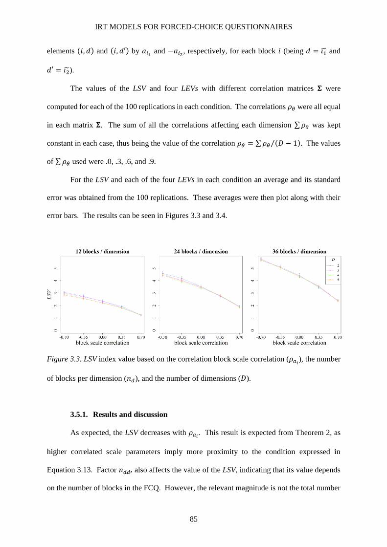
IRT MODELS FOR FORCED-CHOICE QUESTIONNAIRES
85
elements (𝑖, 𝑑) and (𝑖, 𝑑′) by 𝑎𝑖1 and −𝑎𝑖2, respectively, for each block 𝑖 (being 𝑑 = 𝑖1 and
𝑑′ = 𝑖2).
The values of the LSV and four LEVs with different correlation matrices 𝚺 were
computed for each of the 100 replications in each condition. The correlations 𝜌𝜃 were all equal
in each matrix 𝚺. The sum of all the correlations affecting each dimension ∑𝜌𝜃 was kept
constant in each case, thus being the value of the correlation 𝜌𝜃 = ∑𝜌𝜃 (𝐷 − 1)⁄ . The values
of ∑𝜌𝜃 used were .0, .3, .6, and .9.
For the LSV and each of the four LEVs in each condition an average and its standard
error was obtained from the 100 replications. These averages were then plot along with their
error bars. The results can be seen in Figures 3.3 and 3.4.
Figure 3.3. LSV index value based on the correlation block scale correlation (𝜌𝑎𝑖), the number
of blocks per dimension (𝑛𝑑), and the number of dimensions (𝐷).
3.5.1. Results and discussion
As expected, the LSV decreases with 𝜌𝑎𝑖. This result is expected from Theorem 2, as
higher correlated scale parameters imply more proximity to the condition expressed in
Equation 3.13. Factor 𝑛𝑑𝑑′ also affects the value of the LSV, indicating that its value depends
on the number of blocks in the FCQ. However, the relevant magnitude is not the total number

IRT MODELS FOR FORCED-CHOICE QUESTIONNAIRES
86
Figure 3.4. LEV value based on the block scale correlation (𝜌𝑎𝑖), the number of blocks per
dimension (𝑛𝑑), the number of dimensions (𝐷), and the correlation sum per latent trait (∑𝜌𝜃).

IRT MODELS FOR FORCED-CHOICE QUESTIONNAIRES
87
of blocks in the questionnaire, but the number of blocks per dimension. On the other side, the
number of dimensions 𝐷 only affects the LSV slightly when the number of blocks is low. For
24 or more blocks per dimension its effect becomes negligible.
As Equation 3.29 states, the vector of squared singular values of a matrix 𝐗 is equal to
the vector of eigenvalues of its Gramian 𝐗′𝐗. Therefore, if 𝚺 is an identity matrix, the LEV is
equal to the squared LSV. Thus, the values shown in the top row of Figure correspond to the
squares of the values in Figure 3.3. When the latent space correlations 𝜌𝜃 increase, the LEV
increases slightly as well, indicating that the measuring directions of the blocks tend to have
more variability, as illustrated in Figure 3.2. For 𝐷 = 2 and ∑𝜌𝜃 = .9, the value of 𝜌𝜃 is .9—
in this situation, depicted in panels C and F of Figure 3.2, the two dimensions tend to collapse,
making the LEV decrease drastically. These results clearly show the sensitivity of the LEV to
the latent space structure, which the LSV does not account for.
3.6. Simulation Study 2
We conducted another simulation study to test the predictive capability of the
dimensional sensitivity indices. The conditions were chosen in order to generate sufficient
variability in their values while keeping the parameters within a realistic range. Thus, we
expected that the results allowed to compare the quality of the latent trait estimations with the
indices.
We wanted to represent three widespread conditions of item pairing: one where high-
discrimination items have been paired among themselves (and the same for low-discrimination
items), one where the items have been purposely paired in such a way to try to maximize the
directional dispersion of the blocks, and an intermediate one where the items have been
randomly paired. These conditions could stand for three different ways of pairing the same
items, from worst (using a wrong criterion that would yield a low directional variability of the
blocks) to best (carefully pairing the items attending to the magnitude of their scales, in order

IRT MODELS FOR FORCED-CHOICE QUESTIONNAIRES
88
to maximize the directional variability of the blocks). In order to this, we used the procedure
described in Simulation study 1, where the correlation between scales could be manipulated to
simulate the effect of item pairing.
As seen before, the number of blocks per dimension also affects the values of the LSV
and LEV, so it was manipulated as well. The number of latent trait dimensions however affects
neither of them, so its value was kept constant to three, given it is the minimum number of
dimensions that solves the rotational underidentification of the MUPP-2PL (Morillo et al.,
2016). Finally, as the correlations between latent trait dimensions affect the LEV—and
presumably the accuracy of the estimation (Brown & Maydeu-Olivares, 2011)—it was
manipulated as well, following Morillo et al. (2016).
3.6.1. Design and method
The following factors were manipulated: (1) the number of blocks (𝑛), with levels 18
and 36 (i.e., 6 and 12 blocks per pair of dimensions, respectively); (2) the correlation between
the block scale parameters (𝜌𝑎𝑖) with levels -.7, .0, and .7, and (3) the latent trait correlations
(𝜌𝜃) with levels .00, .25, and .50. For each of the 18 conditions resulting from the complete
crossing of these three factors, 100 replications were generated. For each replication, 1,000
respondents to a DBP FCQ were simulated, using the following procedure. First, 1,000 latent
trait vectors were sampled from a trivariate normal distribution with a null vector as mean and
a covariance matrix 𝚺, where the variances were equal to one and all the covariances were
equal to the level of 𝜌𝜃. Second, 𝑛 blocks were generated; scale parameters were sampled with
the procedure and parameters described in Simulation study 1, choosing the off-diagonal
elements of the distribution log-variance parameter such that the correlation between the scales
was equal to 𝜌𝑎𝑖 . Intercept parameters were sampled from a univariate normal distribution,
with mean 0 and variance 0.25. For each replication, the LSV was computed from the block
scale parameters, and the LEV from these and the matrix 𝚺. Finally, a matrix of responses to

IRT MODELS FOR FORCED-CHOICE QUESTIONNAIRES
89
the FCQ was simulated, with the response probability for each person and block modeled by
the MUPP-2PL.
Latent trait estimates were computed using a MCMC procedure similar to Morillo et
al.’s (2016), but setting the structural parameters (block parameters and latent trait covariance
matrix) to their true values. 25.000 samples from the posterior distribution were drawn from
each of four independent chains. The first 10,000 samples from each chain were discarded as
burn-in, and one in 25 of the remaining 15,000 were kept, making a total amount of 2,400
samples from each posterior distribution. The �� convergence statistic (Gelman & Rubin, 1992)
was less than 1.02 for all parameters in all of the replications. From the posterior distribution
samples, the EAP estimate of each respondent latent trait vector was obtained.
3.6.2. Data analysis
The following statistics were computed for each replication:
(a) The mean reliability (𝜌𝜃��2 ) as an indicator of the estimate precision, computed
as the average of the squared correlations between the latent trait parameters and their EAP
estimators.
(b) The mean correlation bias (∆𝜃��𝑟) as an indicator of the distortion of the
dimensionality of the estimates, computed as the average difference between the correlations
of the true latent trait parameters and the correlations of the EAP estimates. (Note that
negatively biased correlations between the estimates indicate a trend to artificially induce
collinearity in the EAP estimates.)
For each of these statistics a three-way ANOVA with the three factors as independent
variables was conducted. To assess the capability of the LSV and LEV to forecast the
dimensionality of the estimates, their correlations with ∆𝜃��𝑟 were computed. Their
relationship with ∆𝜃��𝑟 was also explored graphically to make a more accurate interpretation.

IRT MODELS FOR FORCED-CHOICE QUESTIONNAIRES
90
All simulations, estimations and statistical analyses were performed using R software, version
3.1.2, except the analyses of variance, which were made with IBM SPSS version 20.
3.6.3. Results
3.6.3.1. Analysis of Variance
Given the statistical power of the simulation study, all effects were significant (α = .05)
in both analyses. Therefore, we focus the analysis of the results on the large-size effects,
according to Cohen’s (1988) criterion of a cutoff value of .14 for the 𝜂𝑃2 statistic.
Table 3.1.
Marginal means of the statistics and main effect sizes
of the three-way ANOVA.
𝜌��2 ∆𝜃��𝑟
Number of blocks (𝑛)
18 0.618 -0.211
36 0.741 -0.142
𝜂𝑃2 .759 .356
Block scale correlation (𝜌𝑎𝑖)
-.7 0.755 -0.076
0 0.705 -0.135
.7 0.579 -0.319
𝜂𝑃2 .819 .829
Latent trait correlations (𝜌𝜃)
.00 0.704 -0.216
.25 0.673 -0.193
.50 0.661 -0.120
𝜂𝑃2 .211 .431
Note. 𝜌��2 = Mean reliability; ∆𝜃��𝑟 = Mean
correlation bias; 𝜂𝑃2 = Observed effect size for the
main effect of each factor.

IRT MODELS FOR FORCED-CHOICE QUESTIONNAIRES
91
Table 3.1 shows the main effects marginal means estimated by the analyses, along with
their effect sizes. All major effects were large; on the contrary, all of the interaction effects
had sizes below .14, except for the interaction between 𝜌𝑎𝑖 and 𝜌𝜃 for the 𝜌��2 (𝜂𝑃
2 = .233). As
shown in Table 3.1, 𝜌��2 was higher for 𝑛 = 36 than 𝑛 = 18. The interaction between 𝜌𝑎𝑖 and 𝜌𝜃
for this statistic is shown in Figure 3.5. In general, 𝜌��2 decreased with the values of both 𝜌𝑎𝑖
and 𝜌𝜃. However, there was barely any difference for 𝜌𝑎𝑖 = -.7, while for 𝜌𝑎𝑖 = .7, 𝜌��2 was
lower the higher the value of 𝜌𝜃.
As for ∆𝜃��𝑟, its value was negative for all conditions. Its absolute value was greater
for 𝑛 = 18 than for 𝑛 = 36. It also increased with the value of 𝜌𝑎𝑖 , and decreased with the value
of 𝜌𝜃. Interestingly, the results for ∆𝜃��𝑟 went in the same direction as 𝜌��2 , except for the latter.
Also, contrary to 𝜌��2 , no relevant interaction effect was found between 𝜌𝑎𝑖, and 𝜌𝜃 (𝜂𝑃
2 = .069).
Figure 3.5. Interaction between the effects of the block scale correlation (𝜌𝑎𝑖) the latent trait
correlations (𝜌𝜃) on the mean reliability (𝜌��2 ). LTC = latent trait correlations.
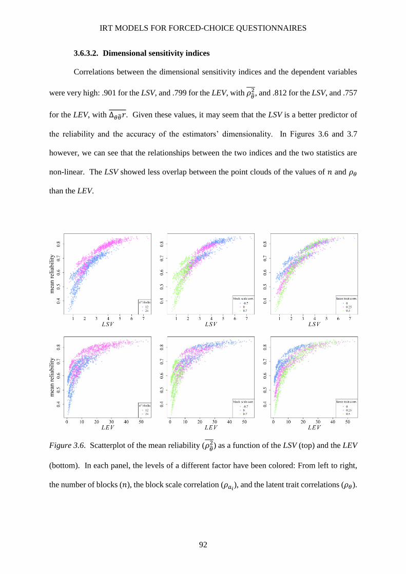
IRT MODELS FOR FORCED-CHOICE QUESTIONNAIRES
92
3.6.3.2. Dimensional sensitivity indices
Correlations between the dimensional sensitivity indices and the dependent variables
were very high: .901 for the LSV, and .799 for the LEV, with 𝜌��2 , and .812 for the LSV, and .757
for the LEV, with ∆𝜃��𝑟. Given these values, it may seem that the LSV is a better predictor of
the reliability and the accuracy of the estimators’ dimensionality. In Figures 3.6 and 3.7
however, we can see that the relationships between the two indices and the two statistics are
non-linear. The LSV showed less overlap between the point clouds of the values of 𝑛 and 𝜌𝜃
than the LEV.
Figure 3.6. Scatterplot of the mean reliability (𝜌��2 ) as a function of the LSV (top) and the LEV
(bottom). In each panel, the levels of a different factor have been colored: From left to right,
the number of blocks (𝑛), the block scale correlation (𝜌𝑎𝑖), and the latent trait correlations (𝜌𝜃).
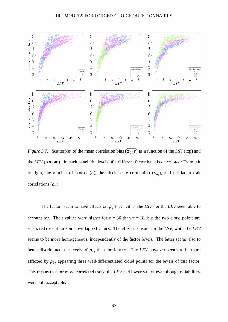
IRT MODELS FOR FORCED-CHOICE QUESTIONNAIRES
93
Figure 3.7. Scatterplot of the mean correlation bias (∆𝜃��𝑟) as a function of the LSV (top) and
the LEV (bottom). In each panel, the levels of a different factor have been colored: From left
to right, the number of blocks (𝑛), the block scale correlation (𝜌𝑎𝑖), and the latent trait
correlations (𝜌𝜃).
The factors seem to have effects on 𝜌��2 that neither the LSV nor the LEV seem able to
account for. Their values were higher for 𝑛 = 36 than 𝑛 = 18, but the two cloud points are
separated except for some overlapped values. The effect is clearer for the LSV, while the LEV
seems to be more homogeneous, independently of the factor levels. The latter seems also to
better discriminate the levels of 𝜌𝑎𝑖 than the former. The LEV however seems to be more
affected by 𝜌𝜃, appearing three well-differentiated cloud points for the levels of this factor.
This means that for more correlated traits, the LEV had lower values even though reliabilities
were still acceptable.

IRT MODELS FOR FORCED-CHOICE QUESTIONNAIRES
94
Regarding ∆𝜃��𝑟, both indices similarly discriminated the conditions for 𝜌𝑎𝑖 = .7, and
were insensitive to the levels of 𝑛 and 𝜌𝜃. In the case of the LEV, for the combination of 𝑛 = 18
with 𝜌𝜃 = .50 there were replicas with a very close-to-zero ∆𝜃��𝑟 (being its value even positive
in some of them), that had a relatively low LEV nevertheless, in the range of about 5 to 15.
This effect also happened for the LSV (with values between 2 and 4), though less pronounced.
Table 3.1 shows that this condition was very favorable for recovering non-distorted
correlations. However, as seen in the lower row of Figure 3.4, for correlations like these, which
sum up to 1 for each latent trait, the LEV started to get lower.
3.6.4. Discussion
We can reach to three main conclusions from the results of the analyses of variance.
First, when we approach the situation expressed Theorems 1 and 2 (i.e., the block scale
parameters are more positively correlated), the estimates are less reliable. The correlations
among the latent trait estimates are also more distorted in this situation, being more negative
than the correlations between the true parameters. Second, increasing the number of blocks
measuring each dimension not only improves the reliability of the estimates, but reduces the
distortion of their correlations. Finally, a positive correlation between the latent traits
undermines the reliability, but gives estimates that better respect the structure of the latent
space. This implies that the marginal information of the latent trait estimates is somewhat
lower, while the estimation errors are less correlated. This is consistent with the theoretical
predictions, as the directional distribution of the blocks improves with positive correlations.
However, the blocks MBSs get lower with increasing latent trait correlations, thus undermining
the empirical reliabilities.
Regarding the dimensional sensitivity indices, both of them are more strongly related
with the mean correlation bias than with the reliability. This result was expected, given that
both indices are supposed to inform of the latent space distortion. The LSV has a higher positive
IRT MODELS FOR FORCED-CHOICE QUESTIONNAIRES
95
correlation with the mean correlation bias than the LEV, so it seems to be a better predictor of
the latent space distortion, in principle. However, the non-linearity among the relationships of
these indices explains this phenomenon. The LEV is in fact less affected by variables that are
irrelevant to the dimensional sensitivity of the FCQ, namely, the latent trait correlations and
the questionnaire length. This allows a clearer cutoff for a quality criterion.
Although this simulation proves the effect of item pairing on the quality of the
estimations, we should highlight the limitations to the external validity of the results. The
dimensional sensitivity of a FCQ may be manipulated in some other ways apart from the
correlation between the block scale parameters. In the simulation studies we have kept the
marginal distributions constant, although both their central tendency and variability may affect
the results as well. Other manipulations may represent empirical situations more faithfully,
which may yield to better understanding on the behavior of the FCQs and the dimensional
sensitivity indices we have proposed.
3.7. General discussion
In this study we have proposed a way to design FCQs robust against the SD bias. The
DBP design involves the use of bidimensional, homopolar-direct blocks; these conditions are
arguably necessary—though not sufficient—for controlling this bias effectively. However, we
have proven that the MUPP-2PL model is likely to be empirically underidentified for a
questionnaire designed under these criteria. In sight of these results, several points deserve
special attention.
3.7.1. DBP design of forced-choice questionnaires
One may argue that the DBP conditions are not strictly necessary to design a SD-robust
FCQ. Indeed, when a FCQ combines homopolar and heteropolar blocks, the directional
variability of the blocks is much better and thus poses no issues of dimensional restriction. The
condition of only homopolar blocks exclusively comes from the consideration that there is a

IRT MODELS FOR FORCED-CHOICE QUESTIONNAIRES
96
socially desirable pole on each trait scale. That is, social desirability is a monotonical function
of the latent trait value.
There is evidence that for extremely high levels of desirable traits, the outcome may
actually be negative; this phenomenon has been termed the too-much-of-a-good-thing effect
(Pierce & Aguinis, 2013). For example, Conscientiousness is considered one of the most valid
and most general predictors of job performance (Barrick, Mount, & Judge, 2001). However,
for very high levels, the relationship with performance becomes negative (Le et al., 2011).
Arguably, this is caused by paying too much attention to small details in detriment of more
important goals (Mount, Oh, & Burns, 2008), and adhering too rigidly to rules, thus inhibiting
adaptation to changes (Le Pine, Colquitt, & Erez, 2000). Previous research also states that job
applicants’ implicit theories may account for this curvilinear relationship, and thus those
applicants may avoid endorsing response categories that are too high on a trait continuum
(Kuncel & Tellegen, 2009).
In conclusion, we may hypothesize that, for a high location in the socially desirable
pole of a scale, inverses items may actually be more desirable than direct ones. Pairing such
inverse items with direct items may lead to SD-robust blocks. Therefore, one could assemble
SD-robust FCQs without restricting the choice to homopolar blocks. Exploring this possibility
is a challenge that may be addressed by future research.
3.7.2. MUPP-2PL empirical underidentification
Simulation study 2 leads to the conclusion that the distribution of the scale parameters
may be close to the empirical underidentification. In such a circumstance, the distortion in the
IRT estimates are similar to those affecting the ipsative scores reported by Meade (2004).
However, when the items are carefully paired, such that the correlation of the block scales is
low (or even negative), both the reliability and the correlations of the latent traits are good
enough, even with as low as 12 blocks per dimension. These results go against Brown and

IRT MODELS FOR FORCED-CHOICE QUESTIONNAIRES
97
Maydeu’s (2011, p. 489) assertion that 12 blocks per dimension would give below-standard
precisions, despite the quasi-equivalence of the MUPP-2PL and the TIRT models.
There are two factors that may explain these divergent conclusions. In first place, they
make this particular assertion from a FCQ intended to measure a five-dimensional latent space.
As we saw in Simulation study 2, higher correlations lead to lower reliabilities. Given the
values of the correlations used in their Simulation study 2 (Brown & Maydeu-Olivares, 2011,
p. 486), we can expect the reliabilities they obtain to be even lower. In fact, there is a negative
relationship between the reliability of each dimension and the sum of its correlations (see the
results for actual reliability in Table 7, p. 488).
More important than that is the difference between the scale parameter distributions
used. There are relevant differences in the absolute values: The mean of the marginal
distributions were 1.433 in our study; in theirs (p.479) they were 1.6993 when the factor
loadings are translated into the logistic IRT metric (the mean sample values for the two
dimensions were 1.532 and 1.506 respectively, see Table 1 in Brown & Maydeu-Olivares,
2011, p. 477). Even though the expected values are higher in theirs, it is the correlation among
these parameters which plays a critical role in this phenomenon. As the authors points out,
when factor loadings of utilities are similar, the model cannot be identified in
respect to factor covariances—one factor collapses. So, looking at these old
simulations now . . . . I would have made factor loadings much more different
in +/+ condition. (A. Brown, personal communication, March 28, 2014).
In fact, the factor loadings they used for their simulations, when translated to IRT metric, have
an expected correlation of .785 (see Footnote 1) being .666 their sample correlation. This is
even closer to the empirical underidentification than the one we used in Simulation study 2.
3 Both the mean of the marginal distributions and the correlation were estimated by simulation, using 107
replications (all Monte Carlo errors < 5×10⁻⁵).

IRT MODELS FOR FORCED-CHOICE QUESTIONNAIRES
98
One important conclusion from this is that, when assembling FCQs following a DBP
design, one must take care to get as far as possible from the empirical underidentification. One
way to achieve this is by pairing some low-discrimination and high-discrimination items in the
same block and, in other blocks addressing the same dimensions, high-discrimination with low-
discrimination items. The resulting FCQ should have enough variability of the block directions
to avoid that they are close to being proportional (as in Equation 3.13). This recommendation
becomes especially relevant when the choices are limited by the pool of items to be paired, as
these will already set an upper bound to the marginal information that can be achieved in each
latent dimension. Thus, the only way to achieve lower estimation errors and less dimensionally
distorted latent trait estimates is by pairing the items wisely to maximize the directional
dispersion of the questionnaire information.
On the other hand, note that, despite these caveats, correlations among latent trait
estimates tend to be more negative than they should. For this reason, using the EAP estimators
as input variables for other models should be done carefully, since their correlations will almost
certainly be distorted. When designing a FCQ for a certain application, the test practitioner or
the researcher may want to have a clear idea of the application it is intended for beforehand—
depending on it, they may be more interested in maximizing the reliability, the construct
validity of the scores (by reducing the correlational distortion among them) or both.
3.7.3. Dimensional sensitivity indices
The proposed dimensional sensitivity indices show reasonable properties to predict the
distortion in the latent trait correlations. When the test designer has prior knowledge on the
items that will be used to create a questionnaire (e.g. the factor loadings in applications with
Likert-type scales) they can use it to estimate the LSV. If knowledge about the latent space
structure is also available, it would be advisable to obtain an estimate of the LEV. As a quality
criterion, we propose cutoffs of about 3 for the LSV and 10 for the LEV. These values,

IRT MODELS FOR FORCED-CHOICE QUESTIONNAIRES
99
according to our results, give a lower bound of the mean latent trait correlation distortions of
about -.2. (Note that in Figures 3.6 and 3.7 these values screen out all the conditions where
BSC = -.7).
Two things are noteworthy regarding the dimensional sensitivity indices however:
First, these indices are useful to provide evidence that a FCQ is well designed. However, even
for well-designed DBP questionnaires they may give below-standard values; this may lead to
false rejections of FCQs that actually have a proper design. This is especially true when there
are few blocks per dimension, as seen in the results of Simulation study 2. Second, it should
be noted that the two indices are rather general; neither of them provides an accurate insight
about the estimation quality for more local aspects of the latent space. They also disregard the
information provided by the block intercept parameters, which may be critical when we want
to maximize the questionnaire quality in certain regions of the latent space. Also, it may be
interesting to propose indexes that focus on diagnosing the quality of the questionnaire for
specific latent dimensions.
3.7.4. Generalization of the results
The algebraic equivalence between the MUPP-2PL and the MCLM model opens doors
to a possible extrapolation of the results presented here to the latter model. The results
presented here generalize Ackerman’s assertion to other situations that may also affect other
realizations of the MCLM. Moreover, the quasi-equivalence to the TIRT model allows a
possible generalization of some of these results to it, at least regarding two-item blocks.
The possibility of applying these results to formats with more than two items per block
as well can be a future research line. Indeed, Brown (2016) reports identification issues when
using latent factor models with certain special properties, and gives an example of a FCQ with
three triplets measuring three latent dimensions. Our results give a rationale for the case of

IRT MODELS FOR FORCED-CHOICE QUESTIONNAIRES
100
paired blocks, and may explain that a DPB design yields to convergence issues in certain
scenarios (e.g., Simulation study 1 in Brown & Maydeu-Olivares, 2011).
Of course, whether these generalizations are valid or not is still an open question. For
other models like the original MUPP (Stark et al., 2005) for example, it is unknown how the
variability in the discrimination parameters can affect the empirical identification of the model.
This may be also a future research line.

IRT MODELS FOR FORCED-CHOICE QUESTIONNAIRES
101
References
Ackerman, T. A. (1994). Creating a test information profile for a two-dimensional latent space.
Applied Psychological Measurement, 18(3), 257–275.
doi:10.1177/014662169401800306
Barrick, M. R., Mount, M. K., & Judge, T. A. (2001). Personality and performance at the
beginning of the new millennium: What do we know and where do we go next?
International Journal of Selection & Assessment, 9(1/2), 9–30. doi:10.1111/1468-
2389.00160
Brown, A. (2016). Item response models for forced-choice questionnaires: A common
framework. Psychometrika, 81(1), 135–160. doi:10.1007/s11336-014-9434-9
Brown, A., & Maydeu-Olivares, A. (2011). Item response modeling of forced-choice
questionnaires. Educational and Psychological Measurement, 71(3), 460–502.
doi:10.1177/0013164410375112
Chernyshenko, O. S., Stark, S., Prewett, M. S., Gray, A. A., Stilson, F. R., & Tuttle, M. D.
(2009). Normative scoring of multidimensional pairwise preference personality scales
using IRT: Empirical comparisons with other formats. Human Performance, 22(2),
105–127. doi:10.1080/08959280902743303
Christiansen, N. D., Burns, G. N., & Montgomery, G. E. (2005). Reconsidering forced-choice
item formats for applicant personality assessment. Human Performance, 18(3), 267–
307. doi:10.1207/s15327043hup1803_4
Clemans, W. V. (1966). An analytical and empirical examination of some properties of ipsative
measures. In Psychometric Monograph. Richmond, VA: Psychometric Society.
Retrieved from https://www.psychometricsociety.org/sites/default/files/pdf/MN14.pdf
IRT MODELS FOR FORCED-CHOICE QUESTIONNAIRES
102
Cornwell, J. M., & Dunlap, W. P. (1994). On the questionable soundness of factoring ipsative
data: A response to Saville & Willson (1991). Journal of Occupational &
Organizational Psychology, 67(2), 89–100. doi:10.1111/j.2044-8325.1994.tb00553.x
Eckart, C., & Young, G. (1936). The approximation of one matrix by another of lower rank.
Psychometrika, 1(3), 211–218.
Gelman, A. E., & Rubin, D. B. (1992). Inference from iterative simulation using multiple
sequences. Statistical Science, 7(4), 457–472. doi:10.1214/ss/1177011136
Gentle, J. E. (2007). Matrix algebra: theory, computations, and applications in statistics. New
York: Springer.
Harman, H. H. (1970). Modern Factor Analysis (2nd. ed. rev). Chicago London: The
University of Chicago Press.
Hooper, A. C. (2007). Self-presentation on personality measures in lab and field settings: A
meta-analysis. University of Minnesota, Ann Arbor, Ml.
Kendall, M. (1979). The advanced theory of statistics (4th ed). London: Charles Griffin &
Company Limited.
Kuncel, N. R., & Tellegen, A. (2009). A Conceptual and Empirical Reexamination of the
Measurement of the Social Desirability of Items: Implications for Detecting Desirable
Response Style and Scale Development. Personnel Psychology, 62(2), 201–228.
doi:10.1111/j.1744-6570.2009.01136.x
Le, H., Oh, I.-S., Robbins, S. B., Ilies, R., Holland, E., & Westrick, P. (2011). Too much of a
good thing: Curvilinear relationships between personality traits and job performance.
Journal of Applied Psychology, 96(1), 113–133. doi:10.1037/a0021016
Le Pine, J. A., Colquitt, J. A., & Erez, A. (2000). Adaptability to changing task contexts: Effects
of general cognitive ability, conscientiousness, and openness to experience. Personnel
Psychology, 53(3), 563–593. doi:10.1111/j.1744-6570.2000.tb00214.x

IRT MODELS FOR FORCED-CHOICE QUESTIONNAIRES
103
Lord, F. M., & Novick, M. R. (1968). Statistical theories of mental test scores. Addison-Wesley
Pub. Co.
Maydeu-Olivares, A., & Brown, A. (2010). Item response modeling of paired comparison and
ranking data. Multivariate Behavioral Research, 45(6), 935–974.
doi:10.1080/00273171.2010.531231
McCloy, R. A., Heggestad, E. D., & Reeve, C. L. (2005). A silk purse from the sow’s ear:
Retrieving normative information from multidimensional forced-choice items.
Organizational Research Methods, 8(2), 222–248. doi:10.1177/1094428105275374
McKinley, R. L., & Reckase, M. D. (1982). The use of the general Rasch model with
multidimensional item response data. Retrieved from http://eric.ed.gov/?id=ED227162
Meade, A. W. (2004). Psychometric problems and issues involved with creating and using
ipsative measures for selection. Journal of Occupational and Organizational
Psychology, 77(4), 531–551. doi:10.1348/0963179042596504
Morillo, D., Leenen, I., Abad, F. J., Hontangas, P., De la Torre, J., & Ponsoda, V. (2016). A
dominance variant under the Multi-Unidimensional Pairwise-Preference framework:
Model formulation and Markov Chain Monte Carlo estimation. Applied Psychological
Measurement, 40(7), 500–516. doi:10.1177/0146621616662226
Mount, M. K., Barrick, M. R., Scullen, S. M., & Rounds, J. (2005). Higher-order dimensions
of the Big Five personality traits and the Big Six vocational interest types. Personnel
Psychology, 58(2), 447–478. doi:10.1111/j.1744-6570.2005.00468.x
Mount, M. K., Oh, I.-S., & Burns, M. (2008). Incremental validity of perceptual speed and
accuracy over general mental ability. Personnel Psychology, 61(1), 113–139.
doi:10.1111/j.1744-6570.2008.00107.x
Pierce, J. R., & Aguinis, H. (2013). The too-much-of-a-good-thing effect in management.
Journal of Management, 39(2), 313–338. doi:10.1177/0149206311410060

IRT MODELS FOR FORCED-CHOICE QUESTIONNAIRES
104
Reckase, M. D. (1985). The difficulty of test items that measure more than one ability. Applied
Psychological Measurement, 9(4), 401–412. doi:10.1177/014662168500900409
Reckase, M. D. (2009). Multidimensional item response theory. New York: Springer.
Reckase, M. D., & McKinley, R. L. (1991). The discriminating power of items that measure
more than one dimension. Applied Psychological Measurement, 15(4), 361–373.
doi:10.1177/014662169101500407
Stark, S., Chernyshenko, O. S., & Drasgow, F. (2005). An IRT approach to constructing and
scoring pairwise preference items involving stimuli on different dimensions: The Multi-
Unidimensional Pairwise-Preference model. Applied Psychological Measurement,
29(3), 184–203. doi:10.1177/0146621604273988
Tarmast, G. (2001). Multivariate log–normal distribution. Presented at the ISI Proceedings:
Seoul 53rd Session, Seoul. Retrieved from http://bfi.cl/papers/Ghasem%201998%20-
%20Multivariate%20log-normal%20distribution.PDF
van der Linden, D., te Nijenhuis, J., & Bakker, A. B. (2010). The general factor of personality:
A meta-analysis of Big Five intercorrelations and a criterion-related validity study.
Journal of Research in Personality, 44(3), 315–327. doi:10.1016/j.jrp.2010.03.003
Zhang, J., & Stout, W. (1999). The theoretical DETECT index of dimensionality and its
application to approximate simple structure. Psychometrika, 64(2), 213–249.

IRT MODELS FOR FORCED-CHOICE QUESTIONNAIRES
105
Chapter 4: Testing the invariance assumption of the MUPP-2PL model
Abstract
The formulation of the MUPP-2PL model for multidimensional forced-choice questionnaires
makes two assumptions, that we call measurement and independence assumption. Their
combination leads to the invariance assumption, which implies that the block parameters can
be predicted from the parameters of the items applied in a single-stimulus or graded-scale
format. This study tests the invariance assumption empirically, comparing the parameter
estimates of both formats. We applied a total of 226 items designed to address the Big Five
personality dimensions to a sample of 705 undergraduate students. These same items were
paired in bidimensional forced-choice blocks and applied to a subsample of 396 of the previous
participants. We fit a bi-factor model to the items first, in order to estimate the condition of
sufficient unidimensionality. Then, a general model with the items and blocks was fit using
the Maximum Likelihood estimation with robust error estimates. We tested the equivalence of
the block parameter estimates and their predictions from the item parameters estimating a
restricted model for each parameter and applying a Likelihood Ratio test, computing the
strictly-positive Satorra-Bentler chi-square statistic. The assumption was found to hold
reasonably well, especially for the scale (i.e., discrimination) parameters. In the cases it was
violated, we explored the likely factors that lead to violations of the invariance assumption in
the different parameters. We conclude discussing the practical implications of the results, and
discussing the formulation of accurate hypotheses for testing the violations of the invariance
assumption.
Keywords: forced-choice questionnaires, invariance, IRT, Likelihood Ratio test, MUPP-2PL.

107
Chapter 4:
Testing the invariance assumption of the
MUPP-2PL model
Forced-choice Questionnaires (FCQs) are a type of psychological measurement
instruments used in the evaluation of non-cognitive traits such as personality, preferences and
attitudes (see e.g., Saville & Willson, 1991). However, its use has been limited to very specific
applications due to the ipsativity of the direct scores they yield (Cattell, 1944). Ipsativity is a
property that has three consequences: (1) the violation of the Classical Test Theory assumptions
(Hicks, 1970), (2) a distortion of the reliability and construct validity, and (3) the impossibility
of making between-person comparisons (Cornwell & Dunlap, 1994).
Some authors have recently proposed Item Response Theory (IRT) models as an
alternative to direct scoring. These would allow obtaining normative estimates of the trait
levels. The MUPP model (Stark, Chernyshenko, & Drasgow, 2005) was the first of these
proposals; it is characterized mainly by being a model for two-item blocks, and by assuming
that each item’s measurement model is an ideal point model. The Thurstonian IRT model
(TIRT; Brown & Maydeu-Olivares, 2011), based on Thurstone's Law of Comparative

IRT MODELS FOR FORCED-CHOICE QUESTIONNAIRES
108
Judgment (1927), followed in chronological order. It is applicable to blocks with more than
two items, and assumes a dominance measurement model—the probability of agreement with
each response option follows a cumulative normal probability function.
The MUPP-2PL model (Morillo et al., 2016) is a variant of the MUPP; as such, it
applies to two-item blocks as well. It differs from the original MUPP in that the probability of
agreement with each response option is modeled by a dominance function: it assumes that a 2-
parameter logistic (2PL; Birnbaum, 1968) curve models the responses to each item. As a
consequence, this model is a special case of the more general Bradley-Terry-Luce model
(Bradley & Terry, 1952; Luce, 1959). Given the similarity between a logistic model and a
cumulative normal probability model (Haley, 1952), the MUPP-2PL and the TIRT models are
almost equivalent when applied to paired items (Brown, 2016; Morillo et al., 2016).
The assumptions the MUPP-2PL model is based on can be defined as (1) the
measurement assumption, and (2) the independence assumption (Morillo et al., 2016).
According to the first one, the probability that person 𝑗 agrees with item 𝑖𝑝 (where 𝑝 ∈ {1,2}
stands for the item position within the block) would be given by
P (𝑥𝑖𝑝𝑗 = 1|𝛉𝑗) = ϕL (𝑎𝑖𝑝 (𝜃𝑖��𝑗 − 𝑏𝑖𝑝)), (4.1)
where 𝑥𝑖𝑝𝑗 is a random variable indicating the agreement of 𝑗 with item 𝑖𝑝 (with a value of 1 if
they agree, and 0 if they disagree), 𝛉𝑗 the coordinate vector of 𝑗 in the 𝐷-dimensional latent
space 𝛉 assessed by the instrument, ϕL(∙) the logistic function, 𝜃𝑖��𝑗 the component of 𝛉𝑗 in the
dimension 𝑖�� (measured by item 𝑖𝑝), and 𝑎𝑖𝑝 and 𝑏𝑖𝑝 the characteristic parameters of 𝑖𝑝. These
parameters can be interpreted, respectively, as a scale parameter and a location parameter; 𝑎𝑖𝑝
would indicate how sensitive or discriminant 𝑖𝑝 is to differences in 𝜃𝑖��, while 𝑏𝑖𝑝 would be the
point in 𝜃𝑖�� where P (𝑥𝑖𝑝𝑗 = 1|𝛉𝑗) = .5 (i.e., a point of indifference). Note that the fact that

IRT MODELS FOR FORCED-CHOICE QUESTIONNAIRES
109
𝑖𝑝 only measures 𝜃𝑖�� is implicit in the measurement assumption—each item in a forced-choice
(FC) block is unidimensional.
The independence assumption implies that the decisions on the agreement with each
response option are independent events. Note that this does not imply a statistical
independence of the two decision events; i.e., it does not imply that the probability of choosing
each response category is given by the joint probability of the independent decision events.
That could lead to incompatible outcomes. Rather, it means that the response probability is a
combination of the two independent probabilities, as the two agreement decisions are taken
independently of one another. Mathematically, this assumption is expressed as
P𝑖(𝑦𝑖𝑗 = 𝑝|𝛉𝑗) =P(𝑥𝑖𝑝𝑗 = 1|𝛉𝑗)P(𝑥𝑖𝑞𝑗 = 0|𝛉𝑗)
P(𝑥𝑖𝑝𝑗 = 1|𝛉𝑗)P(𝑥𝑖𝑞𝑗 = 0|𝛉𝑗)+P(𝑥𝑖𝑝𝑗 = 0|𝛉𝑗)P(𝑥𝑖𝑞𝑗 = 1|𝛉𝑗), (4.2)
where 𝑦𝑖𝑗 is a variable indicating the item chosen as a response (with a value of 𝑝 if item 𝑖𝑝 is
chosen), and 𝑥𝑖𝑞𝑗 (with 𝑞 ∈ {1,2}, 𝑞 ≠ 𝑝) a random variable indicating the agreement of 𝑗 with
item 𝑖𝑞 (with a value of 1 if they agree, and 0 if they disagree), being 𝑖𝑞 the item not chosen as
a response in the pair. Combining both assumptions, the probability of a person 𝑗 to select item
𝑖1 in block 𝑖 made up by items 𝑖1 and 𝑖2, would be given by (Morillo et al., 2016)
P𝑖(𝑦𝑖𝑗 = 1|𝛉𝑗) = ϕL(𝑎𝑖1𝜃𝑖1𝑗 − 𝑎𝑖2𝜃𝑖2𝑗 + 𝑑𝑖), (4.3)
where 𝑑𝑖 is the intersection parameter of 𝑖:
𝑑𝑖 = 𝑎𝑖2𝑏𝑖2 − 𝑎𝑖1𝑏𝑖1. (4.4)
(Note that, unless the design implies repeating items in several blocks, the location parameters
of the items 𝑏𝑖1 and 𝑏𝑖2 are underidentified when presented in a FC format.)
The measurement assumption implies that if an item 𝑖𝑝 were presented independently
in a dichotomous response format, the probability of 𝑗 of agreeing with it would also be given
by Equation 4.1. It follows then that it is possible to present 𝑖1 and 𝑖2 in a dichotomous format
and test whether the parameter of the FC block are equivalent to the parameters of the

IRT MODELS FOR FORCED-CHOICE QUESTIONNAIRES
110
dichotomous items. It also follows from the two MUPP-2PL assumptions that 𝑎𝑖𝑝 is
independent of which other item 𝑖𝑝 is paired with, and that 𝑑𝑖 is a linear combination of the
two independent location parameters 𝑏𝑖1 and 𝑏𝑖2. We call this the invariance assumption, as it
follows that the item and block parameters are invariant to both the format (FC versus
dichotomous) and the within-block context (i.e., which other item a certain item is paired with).
The invariance assumption is prevalent in the design of forced-choice instruments (see,
e.g., Stark et al., 2005), albeit largely untested; the literature has not subjected this assumption
to abundant scrutiny so far. Lin and Brown (2017) performed a retrospective study on massive
data from FCQs applied to personnel selection. Applying the TIRT model, they compared the
parameters in two formats: A partial-ranking task with four items per block (most/least like
me), and a complete-ranking task with three items per block (after dropping one item from each
block). They found that the parameters largely fulfilled the invariance assumption. They also
identified possible sources of bias that might result in a violation of the invariance assumption
and interpreted them as within-block context effects—variations of the item parameters due to
the other item(s) in the same block. However, we should highlight that (1) they did not compare
the FC format with the items individually applied in a graded-scale (GS) format, and (2) one
can argue that context effects are just one amongst many possible sources of lack of invariance.
4.1. A test of the invariance assumption with graded scale items and forced-choice blocks
The traditional format of presenting non-cognitive items in questionnaires is the GS or
Likert format. This format implies a series of responses graded in their level of agreement with
the statement of the item. The Graded Response model (GRM; Samejima, 1968) can be applied
to the data from a GS questionnaire. The additional response categories in the scale (compared
to a dichotomous format) provide additional information that leads to more accurate latent trait
estimates (Lozano, García-Cueto, & Muñiz, 2008). According to the GRM, the response
probability of person 𝑗 to each of the 𝑚 + 1 response categories of item 𝑖𝑝 is given by

IRT MODELS FOR FORCED-CHOICE QUESTIONNAIRES
111
P (𝑥𝑖𝑝𝑗 = 𝑘|𝛉𝑗) =
{
1 − ϕL (𝑎𝑖𝑝
∗ 𝜃𝑖��𝑗 + 𝑔𝑖𝑝𝑘+1) if 𝑘 = 0
ϕL (𝑎𝑖𝑝∗ 𝜃𝑖��𝑗 + 𝑔𝑖𝑝𝑘) − ϕL (𝑎𝑖𝑝
∗ 𝜃𝑖��𝑗 + 𝑔𝑖𝑝𝑘+1) if 0 < 𝑘 < 𝑚
ϕL (𝑎𝑖𝑝∗ 𝜃𝑖��𝑗 + 𝑔𝑖𝑝𝑘) if 𝑘 = 𝑚
, (4.5)
where 𝑥𝑖𝑝𝑗 is a random variable that indicates the response of 𝑗 to the item 𝑖𝑝, 𝑘 ∈ [0,𝑚], 𝑘 ∈
ℤ is the value of 𝑥𝑖𝑝𝑗 indicating a response category, 𝑎𝑖𝑝∗ is the scale parameter of item 𝑖𝑝, and
𝑔𝑖1𝑘 is the intercept parameter for the probability of choosing category 𝑘 or higher in item 𝑖𝑝
(the rest of the symbols defined as in Equations 4.1 and 4.2). Note that when 𝑚 = 1 and there
are two response categories, then Equation 4.5 is reduced to the 2PL model expressed in
Equation 4.1, with 𝑔𝑖𝑝1 = 𝑔𝑖𝑝 = −𝑎𝑖𝑝∗ 𝑏𝑖𝑝.
When 𝑚 > 1, we may consider a recoding of the response 𝑥𝑖𝑝𝑗 to 𝑥′𝑖𝑝𝑗, such that for
an arbitrary response category 𝑘′, 0 < 𝑘′ ≤ 𝑚, 𝑥′𝑖𝑝𝑗 = 0 if 𝑥𝑖𝑝𝑗 < 𝑘′, and 𝑥′𝑖𝑝𝑗 = 1 if 𝑥𝑖𝑝𝑗 ≥
𝑘′. That is, a threshold 𝑘′ can be applied to the responses of the GS item 𝑖𝑝 such that 𝑥′𝑖𝑝𝑗 is
coded as 1 if 𝑥′𝑖𝑝𝑗 is equal to or higher than 𝑘′, and 0 otherwise. This recoding implies
representing the responses to the Likert-type items in a dichotomous format.
According to the GRM, when dichotomizing a GS item, parameter 𝑎𝑖𝑝∗ is expected to
remain unchanged (Samejima, 1968). The location parameter of the dichotomized item
response for threshold 𝑘′ is given by
𝑏𝑖𝑝𝑘′ = −𝑔𝑖𝑝𝑘′ 𝑎𝑖𝑝∗⁄ . (4.6)
Applying Equation 4.6 to Equation 4.4, the intercept parameter 𝑑𝑖 of block 𝑖 can be predicted
from a 𝑑𝑖𝑘′ parameter computed from its items 𝑖1 and 𝑖2, which is expressed as
𝑑𝑖𝑘′∗ = 𝑔𝑖1𝑘′ − 𝑔𝑖2𝑘′. (4.7)
Therefore, we can assume an expected parametric equivalence between a FC block and its
constituent items, given by 𝑎𝑖𝑝 = 𝑎𝑖𝑝∗ and 𝑑𝑖 = 𝑑𝑖𝑘′
∗ for a given threshold category 𝑘′.

IRT MODELS FOR FORCED-CHOICE QUESTIONNAIRES
112
We must make a caveat here, since none of the 𝑏𝑖𝑝𝑘′ parameters can be considered
equivalent to the actual 𝑏𝑖𝑝. As we stated before, the latter represents the point in the 𝜃𝑖��
continuum where P (𝑥𝑖𝑝𝑗 = 1|𝛉𝑗) = .5 in Equation 4.1, when such a statement is presented as
a dichotomous item. When we perform a dichotomization of a GS format as stated above, the
𝑘′ threshold category chosen does not necessarily imply that any of the 𝑏𝑖𝑝𝑘′ parameters
coincide with the 𝑏𝑖𝑝 parameter from the dichotomous presentation as given by Equation 4.6.
We consider however that the equivalence given by the assumptions that lead to Equation 4.6
justify considering and assessing the linear combination of item intercept parameters, as given
in Equation 4.7, as a proxy for the block intercept parameter.
4.2. Aim of the study
Items in personality questionnaires are usually applied in a GS format. In addition, they
hardly ever fit a unidimensional model—rather, personality researchers develop broadband
items that fit a bi-factor model accounting for specific-content facets. To develop a FCQ we
may use the GS item parameters as proxies of the expected block parameters. This may help
us pair the items following proper design criteria, as well as predict the properties of the
resulting questionnaire. However, such a procedure assumes invariance of the block
parameters.
The purpose of this study is thus to test the invariance assumption of the MUPP-2PL
model. In order to this, we will compare the parameters of a set of items designed to measure
personality variables, applying them in the two aforementioned formats: FC, and GS. The
following hypotheses will be tested: (1) the scale parameters of the items (𝑎𝑖𝑝) are independent
of the format (FC or GS), and (2) the intersection parameters of the FC blocks (𝑑𝑖) can be
accurately predicted from a linear combination of the intercept parameters of its items (𝑔𝑖𝑝𝑘)
applied in the GS format.

IRT MODELS FOR FORCED-CHOICE QUESTIONNAIRES
113
Furthermore, we will explore the likely sources of bias that induce violations of the
invariance assumption. We will aim to identify sources of bias at three levels: individual item,
FC block, and questionnaire. Whenever possible, we will try to give tentative explanations to
these phenomena, and discuss further research designs that may allow formulating and testing
precise hypotheses about the violations of the invariance assumption.
4.3. Method
4.3.1. Materials
A dataset consisting of responses to a GS questionnaire and a FCQ was used for this
study. Both instruments shared a large number of items and were answered by a common
group of participants, so they were suitable to verify these hypotheses. The contents of this
dataset are described below.
4.3.1.1. Instruments.
Graded-scale questionnaire. It consisted of 226 GS items presented in a five-point
Likert scale (completely disagree – disagree – neither agree nor disagree – agree – completely
agree). The items were designed to measure the dimensions of the Big Five model (McCrae
& John, 1992), following a bi-factor model. This model assumes a general dimension
representing the substantive trait, as well as six specific dimensions representing residual
variances of item clusters, associated with their content (Holzinger & Swineford, 1937).
Forty-four items were applied for each of the five traits. 122 of these items were direct
(i.e., positively keyed), and 98 were inverse (i.e., negatively keyed; see Chapter 2); polarity
was aimed to be balanced among the different traits, with 22 to 26 direct items and 18 to 22
inverse items per trait. The remaining six items were directed items, applied with the intention
of controlling the quality of each participant’s responses (Maniaci & Rogge, 2014). The items
were distributed in two booklets, with 113 items each, with the directed items at positions 26,
57 and 88, and 23, 55 and 87 in the first and second booklet, respectively.

IRT MODELS FOR FORCED-CHOICE QUESTIONNAIRES
114
Forced-choice questionnaire. A third booklet consisted of 98 FC bidimensional
blocks. Out of them, 79 were made up from items from the GS questionnaire (except for 13
pairs, which contained a direct item from the GS booklets, paired with an inverse item not
included in that instrument). There were also sixteen additional blocks made up by items from
a different application, and three directed blocks (at positions 25, 43 and 76) to control for
response quality. Table 4.1 summarizes the frequency distribution of the FC blocks by pair of
traits. Out of the 79 blocks with items from the GS questionnaire, 24 were formed by two
direct items (homopolar blocks); the remaining 55 were heteropolar, consisting of a direct and
an inverse item, being the direct one always in the first position.
Table 4.1.
Distribution of the FC blocks by trait.
Item 2
Item 1
Neuroticism Extraversion Agreeableness Openness Conscientiousness
Neuroticism
- 3 3 3 3
Extraversion
5 - 5 3 5
Agreeableness
4 3 - 4 5
Openness
5 5 4 - 4
Conscientiousness
5 3 3 4 -
4.3.1.2. Participants
705 undergraduate students from the first and third courses in the Faculty of Psychology
(Autonomous University of Madrid) answered the GS questionnaire on optical mark reader-
ready response sheets. Eight response vectors were dropped due to having too many missing
responses (more than 68), and two more because of failing the directed items (more than one
error). Of the remaining 695, 396 also responded to the FCQ on another optical mark reader-
ready sheet. No response vectors were dropped due to missing responses (only 12 vectors had

IRT MODELS FOR FORCED-CHOICE QUESTIONNAIRES
115
just one missing response), but four were deleted due to failing one or more directed blocks,
leaving 392 valid vectors.
4.3.2. Data analysis
4.3.2.1. Estimation of the latent trait models
The questionnaires were analyzed with multidimensional IRT models using the robust
maximum likelihood (MLR) method (Yuan & Bentler, 2000). 64-bit Mplus 7.0 software
(Muthén & Muthén, 1998-2012) for Windows was used for all analyses. Package
MplusAutomation 0.7-1 (Hallquist & Wiley, 2018) for 64-bit R 3.4.3 (R Core Team, 2017)
was used to automate some of the analysis procedures.
Graded-scale questionnaire. Since the items were designed attending to a bi-factor
model, it was straightforward that unidimensional models would not fit the data. However,
unidimensionality is a necessary condition for the measurement assumption of the MUPP-2PL
to hold. A unidimensional model may be estimated albeit not fitting the data, obtaining
relatively unbiased parameters, as long as the explained common variance (ECV; Ten Berge
& Sočan, 2004) of the general dimension in the bi-factor model is not too low (Rodriguez,
Reise, & Haviland, 2016). Therefore, an exploratory bi-factor model was also estimated for
each dimension in order to diagnose the quality of the unidimensional parameter estimates. Six
specific dimensions and a general one were specified, and an iterative Schmid-Leimann
rotation was applied (Abad, Garcia-Garzon, Garrido, & Barrada, 2017). Taking the scale
parameters on the general dimension as a benchmark for comparison, the correlation, mean
relative bias, and root mean square bias (RMSB) of the unidimensional scale parameters were
computed. The item ECV (I-ECV) index (Stucky, Thissen, & Orlando Edelen, 2013) was also
computed, as a measure of unidimensionality for each item. This index is given by the
proportion of the item common variance explained by the general dimension. Items where
most of the common variance is attributable to this will have an I-ECV close to one; highly

IRT MODELS FOR FORCED-CHOICE QUESTIONNAIRES
116
multidimensional items on the other hand, with common variance highly due to specific facets,
will have I-ECV values close to zero. Given that we assumed the unidimensional models
would fit the data significantly worse than their bi-factor counterparts would, we omitted
testing the significance of the nested model comparisons.
Tests of the invariance assumption. Once the unidimensional models were fit and
their quality assessed (no items had to be dropped due to misspecification), a model was fit to
the item and block responses altogether. Due to computational limitations, models with each
triplet of dimensions were fit in a first place, which included correlated uniquenesses between
each block and its two corresponding GS items. Given that the ML estimation and its variants
don’t allow for correlated uniqueness, these were set by using a two-tier model approach (Cai,
2010), where a common specific dimension was defined where both an item and the FC block
it was in loaded. The loadings on these specific factors were set to 1 for the items, to 1 for the
blocks where that item appeared in the first position, and to -1 for the blocks where it appeared
in the second position.
The resulting unique covariances in those models were non-significant and negligible
in the vast majority of cases, so fitting a model with independent uniquenesses and all the Big-
Five trait dimensions was attempted. However, as had also happened in the tests with
dimension triplets, the full-dimensional model had convergence issues with Extraversion.
Therefore, the items tapping Extraversion and the blocks containing an Extraversion item were
dropped. The responses to the remaining 47 blocks and the 86 GS items included in those were
finally fitted to a model with the remaining four dimensions.
For this model, the block parameter values predicted from the items, 𝑎𝑖𝑝∗ and 𝑑𝑖𝑘′
∗ were
computed. For the intercept parameters, the four possible values of 𝑘′ were used. The block
parameter estimates were correlated with their predictions, and the prediction error was

IRT MODELS FOR FORCED-CHOICE QUESTIONNAIRES
117
obtained for each parameter. The mean error, mean relative error, and root mean square error
(RMSE) were computed for each prediction type.
A constrained model was fit for each possible restriction given by the invariance
assumption: Equal scales for a block and each of its corresponding GS items, and a constraint
on the block and item intercepts given by Equation 4.7 (using the four possible values of 𝑘′).
This would result in six contrasts per block, for a total of 282 constrained models. However,
given that the GS-item parameters were not available for 8 items (out of the 13 taken from a
previous application as explained above, excluding five of them measuring Extraversion), only
the first scale parameter of the corresponding blocks could be tested for invariance, and
therefore 242 constrained models were estimated.
For each of the constrained models, a likelihood ratio test against the unrestricted model
was performed as follows: a strictly positive 𝜒𝑆−𝐵2 statistic (Satorra & Bentler, 2010) was first
computed using the procedure explained by Asparouhov and Muthén (2010). Using a
confidence level of .05, the Bonferroni correction for multiple comparisons was applied to
these tests, giving a value of ∝= . 05 242⁄ = 2.07 × 10⁻⁴. The parameters for which the p-
value of the likelihood ratio test was less than ∝ were considered non-invariant.
4.3.2.2. Exploration of the violations of the invariance assumption
In order to identify possible sources of non-invariance, several factors were considered
and consequently explored. Invariance was studied in terms of significance of the parameter
likelihood ratio test and the absolute deviation from the prediction. At the item level, we
explored whether violations of the measurement assumption lead in turn to violations in the
invariance assumption: Given the items were designed following a bi-factor model, it could be
expected that item multidimensionality (i.e. high loadings on the specific facet dimension)
would affect the invariance assumption through a violation of the MUPP-2PL measurement

IRT MODELS FOR FORCED-CHOICE QUESTIONNAIRES
118
assumption. Also at the item level, item properties (trait measured and polarity) were explored
as possible sources of invariance.
At the block level, we explored the effects of the item properties (dimension and
polarity) when paired together. The properties of a certain item by itself can only affect the
block parameters that depend on that item. Therefore, effects on the parameters that should
depend only on the other item must be necessarily violations of the independence rather than
the measurement assumption.
At the questionnaire level, we studied whether there was any generality that could
explain deviations from the model prediction for all the blocks. For example, FC-format
specific biases affecting could have a differential effect on the parameters as a function of the
item position. Such deviations should be regarded as a general violation of the measurement
assumption. Finally, we analyzed whether there was any association among the invariance of
the different parameter types.
4.4. Results
4.4.1. Dimensionality assessment of the GS questionnaire
The results of assessing the dimensionality of each trait measured by the GS items are
shown in Table 4.2. The ECV was rather low, informing a weak degree of unidimensionality,
especially for the Conscientiousness dimension. However, under certain circumstances, the
parameter estimates from the unidimensional model may be similar enough to the bi-factor
estimates even when unidimensionality is not too strong, even when the unidimensional model
clearly misfits the data (Reise, 2012)4.
Table 4.2 shows that the unidimensional scale estimates correlated strongly with their
bi-factor counterparts, giving evidence of a reasonably good approximation. The histogram in
4 Note that the claims of this author about the percentage of uncontaminated correlations cannot be
directly applied to the present context, as this index makes sense only within the context of confirmatory bi-factor
analysis. However, given the resulting ECVs, the estimates from the unidimensional models were considered apt
to be compared to the bi-factor model estimates, in order to assess their bias.

IRT MODELS FOR FORCED-CHOICE QUESTIONNAIRES
119
Table 4.2.
Diagnostic statistics of the unidimensional GS models, compared to the bi-factor
models.
Dimension ECV (%) Correlation Mean relative bias RMSB
Neuroticism 48.21 .990 -0.098 0.270
Openness to Experience 45.48 .984 -0.051 0.269
Agreeableness 48.52 .988 -0.079 0.207
Conscientiousness 34.44 .987 -0.026 0.218
Note. ECV = Explained common variance; RMSB = Root mean square bias.
Figure 4.1. Distribution of the unidimensional scale parameter estimates of the GS
items, with respect of the general factor scale parameters in the bi-factor models.

IRT MODELS FOR FORCED-CHOICE QUESTIONNAIRES
120
Figure 4.1 shows that the relative bias (in absolute value) was between 0 and 40% in the
majority of cases, with a 69% below 20%. However, some of the values may have been too
biased, being this bias as high as an 84% in a few cases.
Figure 4.2. Scatter plot of the GS items scale parameter estimates, on the general
factor of the bi-factor models and on the common factor in the unidimensional
models.
Figure 4.2 shows the scatter plot of the scale parameter estimates on the unidimensional
model against the corresponding estimates in the general dimension of the bi-factor model. We
can see that the unidimensional estimates had a general bias trend toward zero (i.e. a negative
relative bias). The positive, low-value parameters, on the other hand, had a positive bias trend.

IRT MODELS FOR FORCED-CHOICE QUESTIONNAIRES
121
Figure 4.3 plots the relative bias against the I-ECV, as an indicator of the item relative
unidimensionality. A trend line, computed with a loess smoother (Cleveland & Devlin, 1988)
with a span parameter of .75, is overlaid on the scatter plot. We can clearly identify the two
effects: On one side, the general shrinking trend of around a 10-15% that affected all the items,
regardless of polarity or dimensionality (i.e., an underestimation, in absolute value); on the
other, the stretching trend (or absolute value overestimation) of the items with a low I-ECV.
Arguably, the low discriminating items were the ones mainly affected by multidimensionality,
therefore their positive relative bias (mainly the direct ones, which dominate the
multidimensional end of the spectrum).
Figure 4.3. Scatter plot of the GS items scale parameter relative bias, on the bi-factor
item unidimensionality. I-ECV = item explained common variance. + = positive
(direct item); - = negative (inverse item).

IRT MODELS FOR FORCED-CHOICE QUESTIONNAIRES
122
Summing up, some of the item scale estimates in the unidimensional models might be
too biased for the acceptable standards, which should not be higher than about 15% (Muthén,
Kaplan, & Hollis, 1987). However, they approximated relatively well the ordering of the bi-
factor scale estimates, and we considered them appropriate for the subsequent tests of the
invariance assumption. Nevertheless, we will need to consider these results when interpreting
the comparison of the GS-item parameter estimates with their FC-block counterparts.
4.4.2. Tests of the invariance assumption
The correlations of the block parameter estimates with their predictions from the item
estimates are given in Table 4.3, along with the descriptive statistics of the prediction errors
(columns Correlations through RMSE). Firstly, we can see that the correlations were very high
in all the cases; all of them were above .900 except for the intercept estimates predicted using
the first threshold category. The third threshold category yielded the highest correlation with
the block intercept estimates. Both the mean error and the RMSE of the intercept estimates
Table 4.3.
Summary of results of the invariance assumption tests.
Parameters
Estimate statistics Non-invariant parameters
Correlations Mean error MRE RMSE Count %
Scales .928 -0.132 -0.209 0.355 2 2.33
Intercept (Threshold 1) .870 0.737 -0.335 1.307 13 33.33
Intercept (Threshold 2) .905 0.712 -0.446 1.312 15 38.46
Intercept (Threshold 3) .936 0.521 -0.077 0.780 12 30.77
Intercept (Threshold 4) .908 0.108 -0.157 0.481 10 25.64
Note. MRE = Mean relative error. RMSE = Root mean square error.

IRT MODELS FOR FORCED-CHOICE QUESTIONNAIRES
123
were consistently lower the higher the threshold category was. The mean error was always
positive for the intercept estimates, in contrast to that of the scale parameters, which was
negative. The mean relative error was negative for all cases, manifesting a generalized
underestimation of the block parameters in absolute value. For the intercept estimates, the third
category yielded the lowest mean relative error and, followed by the fourth one. The lowerst
RMSE in contrast was for the fourth category, while it was highest for the first and second one.
Figure 4.4. Scatter plot of the FC-block scale parameter estimates against the
corresponding GS-item estimates. The linear regression trend is shown in yellow. Non-
invariant scale parameters are annotated with the block code.
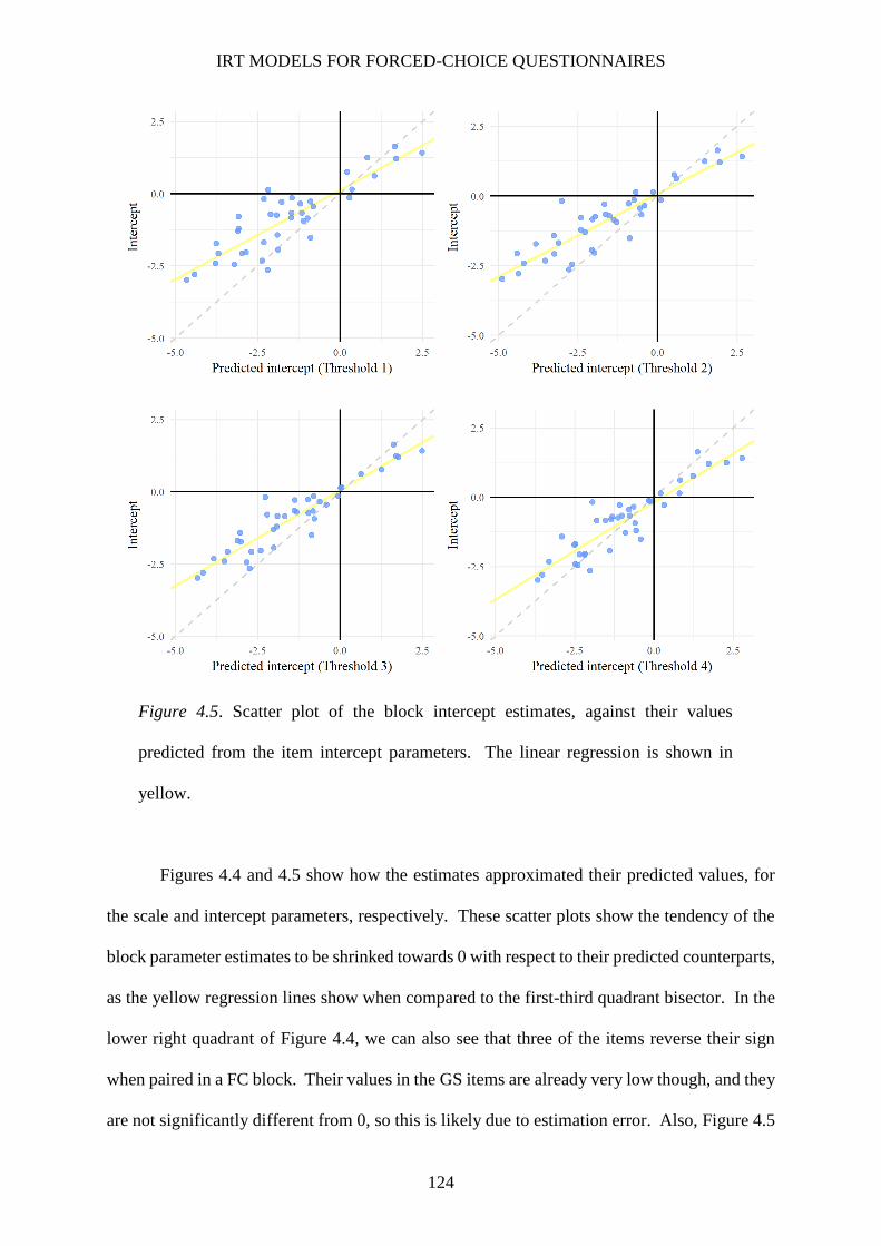
IRT MODELS FOR FORCED-CHOICE QUESTIONNAIRES
124
Figure 4.5. Scatter plot of the block intercept estimates, against their values
predicted from the item intercept parameters. The linear regression is shown in
yellow.
Figures 4.4 and 4.5 show how the estimates approximated their predicted values, for
the scale and intercept parameters, respectively. These scatter plots show the tendency of the
block parameter estimates to be shrinked towards 0 with respect to their predicted counterparts,
as the yellow regression lines show when compared to the first-third quadrant bisector. In the
lower right quadrant of Figure 4.4, we can also see that three of the items reverse their sign
when paired in a FC block. Their values in the GS items are already very low though, and they
are not significantly different from 0, so this is likely due to estimation error. Also, Figure 4.5

IRT MODELS FOR FORCED-CHOICE QUESTIONNAIRES
125
Table 4.4.
Likelihood ratio test statistics of the constrained models.
Block Trait Polarity
Scale 1 Scale 2
Intercept
1 2 1 2 Threshold 1 Threshold 2 Threshold 3 Threshold 4
2 Ne Ag + - 4.265 0.041 4.777 0.973 1.826 0.018
3 Co Ne + + 0.169 13.569 22.846 * 20.248 * 0.781 26.151 *
4 Ne Ag + - 0.698 0.699 0.015 1.556 0.000 0.847
5 Ag Op + - 5.693
6 Op Ne + - 3.363 0.000 22.008 * 43.794 * 2.868 6.674
7 Ne Op + + 0.099 0.008 2.624 2.295 7.616 23.668 *
10 Ne Co + + 1.041 0.652 13.644 7.948 8.705 15.025 *
12 Op Co + + 0.104 0.002 0.465 3.441 1.212 4.470
13 Co Op + + 1.348 4.221 3.492 17.281 * 14.777 * 11.227
14 Ag Co + + 8.297 6.531 0.881 2.005 0.300 0.020
15 Ag Co + - 12.815
16 Op Ag + + 0.000 1.041 2.870 2.102 9.132 9.788
19 Ne Co + - 7.889
20 Op Ne + - 0.167 1.574 7.772 17.802 * 22.843 * 30.441 *
21 Op Co + - 1.950 0.122 13.006 28.849 * 23.758 * 4.177
23 Co Ne + - 0.242 3.264 1.950 30.193 * 18.454 * 27.928 *
24 Co Op + - 2.640 5.480 6.374 4.381 5.259 3.327
27 Op Ne + - 8.053 0.030 1.728 0.377 0.054 3.756
28 Ag Co + - 1.398 0.009 3.492 0.242 0.119 2.590
31 Ag Ne + - 5.134 4.310 43.299 * 24.019 * 14.391 * 12.382
32 Ag Co + + 6.328 1.251 31.139 * 51.424 * 38.602 * 10.792
40 Op Co + - 7.470 0.216 8.832 0.145 3.905 0.294
41 Ne Co + - 11.509
42 Op Ag + - 10.722 0.853 21.150 * 6.823 11.462 1.339
47 Ne Op + - 10.504 0.497 6.830 1.677 1.366 0.190
48 Co Ne + - 6.011 4.612 5.199 14.056 * 17.741 * 16.432 *
50 Co Op + - 0.939 5.427 0.033 9.103 11.148 8.357
51 Co Ag + - 9.630
53 Op Ag + - 6.845
54 Op Co + - 6.777 1.160 55.315 * 112.783 * 73.753 * 120.913 *
56 Ne Ag + + 4.071 5.572 19.170 * 69.386 * 53.257 * 14.807 *
57 Ag Op + - 6.396
58 Co Ag + + 2.342 0.000 16.840 * 0.128 4.143 1.892
59 Ag Ne + - 3.484 9.199 0.662 10.178 19.252 * 19.584 *
61 Ag Op + + 0.982 2.312 0.930 15.908 * 13.339 7.297
64 Ag Op + - 12.368 1.380 0.067 0.309 0.126 6.317
65 Co Op + - 1.216 3.725 7.926 3.754 5.119 0.064
66 Op Ne + + 1.054 4.382 14.746 * 40.338 * 38.894 * 14.396 *
67 Op Ne + - 1.162 0.649 8.776 7.711 4.930 0.169
68 Ne Op + + 6.703 5.239 32.031 * 20.390 * 32.124 * 0.060
69 Ag Ne + + 1.673 0.563 35.046 * 18.378 * 13.353 8.642
71 Op Ag + - 4.791
72 Ag Ne + - 2.761 1.447 22.953 * 13.443 10.677 2.256
73 Co Ag + - 2.178 0.115 5.849 3.716 4.006 2.503
76 Ag Co + - 0.329 6.730 0.750 4.650 0.899 0.186
77 Co Ne + + 27.545 * 5.641 4.086 0.007 0.045 1.289
79 Co Ne + - 0.985 14.054 * 20.062 * 12.814 9.107 8.092
Note. Ne = Neuroticism; Ag = Agreeableness; Op = Openness;
Co = Conscientiousness. * = significant at ∝= 2.07 × 10⁻⁴.

IRT MODELS FOR FORCED-CHOICE QUESTIONNAIRES
126
shows clearly how the third and fourth threshold categories yield better predictions of the block
intercept estimates, as seen in Table 4.3.
The results of the likelihood ratio tests of the constrained models are given in Table 4.4
and summarized in the last two columns of Table 4.3. The null hypothesis of model
equivalence was rejected for only two scale parameters. These are annotated in Figure 4.4 with
their block code, which shows that they have a clearly high, negative deviation from the
predicted value.
In the case of the intercept parameters, their predicted value was not invariant in 10 to
15 cases, depending on the item threshold category considered. The fourth one had the lowest
number of non-invariant parameters, followed by the third one with 12. The second one had
the highest number. The intercept estimate was invariant for all the threshold categories in 17
out of the 39 blocks for which the intercept parameter could be predicted (43.6%). Only in
three of them the intercept parameter was found to be non-invariant for all the categories. The
rest of the blocks had non-invariant intercept parameters in one to three threshold categories.
4.4.3. Exploration of the violations of the invariance assumption
4.4.3.1. Scale parameters
The problem of the likely sources of non-invariance was difficult to address for the
scale parameters, due to the high rate of invariance. Explorations based on the statistical
decision of invariance could not be done, but the value of the prediction error could be explored
in relation to some factors. At the item level, it was plotted against its I-ECV. Visual inspection
revealed no association between the two magnitudes. At the block level, the prediction errors
were also plotted against the I-ECV of the pairing item, revealing no association either. At the
questionnaire level, there only seemed to be the aforementioned general shrinking effect of the
scale values. This could indicate an overall scaling factor affecting the items when presented
in an FC format.

IRT MODELS FOR FORCED-CHOICE QUESTIONNAIRES
127
4.4.3.2. Intercept parameters
Regarding the invariance of the intercept parameters, threshold category used for the
prediction seemed to play a role in its violation. The second category was the one that yielded
less invariant parameters, while the fourth one yielded the more, with only 10 non-invariant
parameters. This pattern was consistent across traits and polarities, as Table 4.5 shows.
Plotting the prediction error of the non-invariant intercept parameters in relation to the
properties of the items and blocks can help study their possible effects on the invariance. This
Table 4.5.
Number of non-invariant intercept parameters per item
trait and block polarity.
Threshold
category
Number of parameters
By trait Total Item 1 Item 2
Neuroticism 1 9 2 7
2 10 2 8
3 8 2 6
4 9 3 6
Openness 1 5 4 1
2 8 5 3
3 6 4 2
4 4 3 1
Agreeableness 1 7 4 3
2 5 4 1
3 4 3 1
4 2 1 1
Conscientiousness 1 5 3 2
2 7 4 3
3 6 3 3
4 5 3 2
By polarity Total Homo. Hetero.
Total 1 13 7 6
2 15 8 7
3 12 5 7
4 10 5 5
Note. Homo. = number of homopolar blocks;
Hetero. = number of heteropolar blocks.

IRT MODELS FOR FORCED-CHOICE QUESTIONNAIRES
128
plot is shown in Figure 4.6. This figure illustrates how most of the intercept parameters had a
positive prediction error, regardless of the traits or polarities of the items involved, or the
threshold category. The fourth category was an exception, as there was an equal number of
positive and negative errors among the non-invariant parameters. Moreover, there was an
association between prediction error sign and polarity for this threshold category, as most of
the negative errors were in homopolar blocks (i.e., with a direct item in second position), while
most of the positive errors were in heteropolar blocks.
In Figure 4.6 we can also study how consistent the test results are across categories in
more detail. Error sign was inconsistent across threshold categories for two blocks (blocks 3
and 56). In most cases, the test was significant either for only one (blocks 7, 10, 58, 61, 42,
72, and 79) or for two categories (blocks 13, 69, 6, 21, and 59). Only two of them were
completely consistent across threshold categories, being significant and with the same sign for
the four of them (blocks 66 and 54), and six (blocks 32, 68, 20, 23, 31, and 48) were consistent
for three of the categories.
Considering these results, the analysis at the item level shows that the traits addressed
may play a role in the violations of the invariance assumption. Neuroticism items were the
most present in blocks where the intercept parameter was non-invariant, followed by Openness.
The less numerous ones were the items tapping Agreeableness. Regarding item
multidimensionality, the intercept error was relatively constant across the different values of
the items I-ECV indicator. Therefore, multidimensionality of the items had no apparent
association with the non-invariance of the intercept parameters.
At the block level, the item position seemed to interact with the trait: Most of the items
tapping Neuroticism in non-invariant blocks were in the second position; in the first position
however, there were less items tapping Neuroticism than other traits. Openness items, on the
other hand, were more prevalent in the first position among those with non-invariant intercept

IRT MODELS FOR FORCED-CHOICE QUESTIONNAIRES
129
Figure 4.6. Deviation of the non-invariant block intercept parameters with respect to their
predicted values from the item intercept parameters.

IRT MODELS FOR FORCED-CHOICE QUESTIONNAIRES
130
parameters. Regarding polarity, given the questionnaire design (with all inverse items in
second place) its effect at the item and block levels could not be studied separately. However,
none of the block polarities had a clear superior effect on the lack of invariance than the other.
Finally, at the questionnaire level, we can see that there is an apparent shrinking effect on the
intercept parameters, similar to the finding in the scale parameters. This may imply a violation
of the measurement assumption given by a scaling factor.
4.5. Discussion
From the results above, we can conclude that, in general, the invariance assumption is
fulfilled in the FC format. Significance testing is highly controversial nowadays, and many
researchers advocate for an analysis of the effect size of the differences (Peng, Chen, Chiang,
& Chiang, 2013; Wilkinson, 1999). In our study, apart from the high rates of invariance, we
found high correlations between the parameters of the two formats, but for some parameters
the difference between the predicted and the estimated values were of a relatively high
magnitude. Nevertheless, we could identify certain phenomena that seem to be involved in the
violations of the invariance assumption. There was a general trend of the parameters to be
underestimated (in absolute value), as the mean relative errors show. Though assuming the GS
items were unidimensional exerted a shrinking effect on their parameters, the block parameters
themselves were even more shrunk with respect to the item parameters in the unidimensional
models. This result points to a likely general violation of the measurement assumption in the
form of a scaling factor, which affects both the scale and the intercept parameters. This
violation would affect all the parameters in a similar fashion, and could be estimated when
assessing the invariance, leading to a hypothesis of partial or conditional invariance.
Apart from that, some of the parameters did not pass the invariance test, yielding
evidence of violations of the invariance assumption. The intercept parameters were the most
affected, whereas only two scale parameters were non-invariant. Due to this low rate of non-

IRT MODELS FOR FORCED-CHOICE QUESTIONNAIRES
131
invariance, the violations of invariance on the scale parameters were difficult to interpret.
Apart from the hypothetical scale shrinking discussed above, no violation of the measurement
assumption seemed to play a specific role in these parameters, given that item
multidimensionality and prediction error were unrelated.
Regarding the intercept parameters, we have seen that the violations of the invariance
assumption depends at least in part on the threshold category used to predict the intercept
parameter values. In fact, only a few estimates deviated from the prediction in a consistent
manner. Arguably, given the central response category was an indifference category (i.e.,
neither agree nor disagree), the more centered a threshold category 𝑘′ was in the GS items, the
closer the location parameters 𝑏𝑖𝑝𝑘′ must have been to the location parameter 𝑏𝑖𝑝 of that item
when presented in a dichotomous format. Therefore, one would think that central categories
should be more reliable predictors. Contrary to this, our results showed that the higher the
category, the better the predictions were, being the third and (specially) the fourth category the
best ones. If higher threshold categories give better predictions of the block intercept
parameter, a violation of the measurement assumption must be taking place, implying the
location parametrs are actually closer to those categories and therefore are negatively biased
when paired in a FC block.
We also found indications that some properties of the items might be affecting the
invariance of the intercept parameters. Neuroticism and Openness seemed to be more involved
in the non-invariant intercept parameters. Moreover, violations of invariance were more
prevalent with Neuroticism items in the second position and Openness items in the first one,
suggesting a complex interaction effect among the two latent traits, item position within the
block, and a possible response bias. Given that most of the intercept parameters were positively
deviated with respect to their prediction, it is likely that such a bias tends to create an attraction
effect on the first item in the block.

IRT MODELS FOR FORCED-CHOICE QUESTIONNAIRES
132
There is another possible explanation however, which would imply violations of both
the measurement and independence assumption. As Figure 4.5 shows, a majority of the
intercept values were negative. Given the aforementioned underestimation of the absolute
values, it is not surprising that most of the non-invariant values had a positive prediction error;
indeed, only four of the intercept estimates that resulted non-invariant for some threshold
category were positive and, unsurprisignly, their predition error was negative. These were
blocks 3, 7, 10, and 13 (see Figure 4.6). However, we have seen that the actual item location
may be negatively biased in the FC blocks. Considering the violations of the invariance, there
are two factors that lead to think the fourth threshold category predictions are more accurate:
First, this category has the least number of non-invariant parameters. Second, it is the only
category that yields evenly distributed positive and negative prediction errors among those.
The remaining threshold categories, however, give a vast majority of positively deviated block
intercepts, which could be explained by the questionnaire-level violation of the measurement
assumption: the combined effects of the scaling factor and the location bias. Finally, a block-
specific effect of the items would induce a violation of the independence assumption, leading
to an increased attractiveness of one item or the other.
If we focus on the fourth threshold category, we see that polarity seems to be associated
with the prediction error sign, as four out of five of the negative errors occur in homopolar
blocks (i.e. were the second item is direct), and the opposite happens in heteropolar blocks.
This would imply that the second item would tend to be relatively more attractive in homopolar
direct blocks, while in heteropolar blocks, the direct item would be relatively less attractive.
In conclusion, if we accounted for the hypothetic general violation of the measurement
assumption (scaling factor and item location bias), the resulting non-invariant parameters
would probably be more interpretable as violations of the independence assumption, possibly
related to the item polarities and measured traits.

IRT MODELS FOR FORCED-CHOICE QUESTIONNAIRES
133
4.6. Conclusions
We have provided evidence that we can assume invariance between the GS and the FC
formats. This fact has a great practical relevance, since it enables building FC blocks based on
the parameters of the individual items. Given that there are many applications of personality
questionnaires in GS formats, our results legitimate the design of FC blocks using the already
known parameters of the items as a proxy for the block parameters. In addition to the obvious
reduction in costs of reusing prior applications of GS questionnaires, this may be useful in
optimizing certain design criteria of FCQs. In addition, if the violations of the invariance
assumption happened to have negligible impact on the measurement, the application of such a
method would be rather straightforward.
Nevertheless, taking into account the possible violations of the invariance assumption
should be paramount for research purposes. Three phenomena may have a relevant effect on
the invariance. First, if solid evidence is found of a shrinking effect, this would be detrimental
to the information of the FCQ (Morillo et al., 2016) and should be consequently considered.
However, it is a constant effect across blocks, and thus should be relatively easy to predict.
Nevertheless, we could obtain a more accurate prediction of this effect by accounting for item
multidimensionality. Extending the MUPP-2PL model in order to consider specific-facet
content would be an improvement in this sense.
Second, we found evidence for a likely bias on the intercept parameters: The high
threshold category values seemed to be better predictors of their values, pointing to a negative
bias of the item location parameters when paired in a FC block. However, this phenomenon
might be interpreted instead as a positive bias in the GS items, such as an acquiescent response
style (Messick, 1966). The exploration of this bias may be an interesting research line, given
the FC format is often claimed to neutralize some response styles endemic to the GS format.

IRT MODELS FOR FORCED-CHOICE QUESTIONNAIRES
134
Applying methods specifically aimed for this purpose, such as random intercept item factor
analysis (Maydeu-Olivares & Coffman, 2006), could help in this sense.
Finally, there is some evidence that blocks tapping certain dimensions and with certain
polarity patterns may be more sensitive to violations of the invariance assumption. These
violations are a rich source of hypotheses on their own. For example, one could apply
experimental FC blocks designed to induce or mitigate non-invariance, and test the subsequent
predictions.
This study has some limitations worth highlighting. Firstly, the available dataset did
not allow for an accurate manipulation of all the relevant factors. Researchers should overcome
two limitations in further studies: (1) To design FCQs that balance the order of the inverse item
in heteropolar blocks, and (2) to calibrate the parameters of the whole item set in both formats.
Using a different response format for the items could also be advantageous, such as an even
number of GS response categories, or a dichotomous format. More complete response vectors
would also be desirable, as the present one was lacking a large amount of responses for the FC
blocks in comparison with the items.
Secondly, the Neuroticism items complicated the interpretation of the results somehow.
We may safely assume that Neuroticism represents the undesirable pole of its dimension (with
Emotional stability in the desirable one), while the remaining traits would be interpreted as
desirable. As stated in Chapter 2, the polarity of a latent dimension is arbitrary, and therefore
one can revert it without any consequence from the modelling point of view. Reframing the
Neuroticism scale as Emotional stability would benefit the interpretation of the parameter
deviations, as we could always identify the positive pole with the desirable one.
Finally, it is worth pointing the problems found when estimating the models with the
Extraversion trait. We could not find convergence due to the latent correlation matrix
becoming singular, as the correlations between the dimension of Extraversion and the others

IRT MODELS FOR FORCED-CHOICE QUESTIONNAIRES
135
approached 1. This may suggest some property of the FC format affecting specifically this
dimension. Whatever the actual explanation is, it should not be overlooked, if we want the
results to be fully extrapolated to the Big Five model, and to other theoretical models the FC
format may be applied to.
Wrapping up, this study introduces a methodology that allows testing the assumptions
of the MUPP-2PL model for paired FC blocks. The application of this method may open up
further research lines, as the ones stated previously. Furthermore, the comparison between FC
blocks and GS could allow for disambiguating between the MUPP-2PL and the TIRT models;
although both models predict similar results when applied to FC blocks, it is not so when the
parameters are compared across response formats. While the invariance in the MUPP-2PL
model is given by the equality of the parameters in an IRT metric, in the TIRT it is given by
their equality in a factorial metric. In conclusion, we expect this proposal to contribute to
developing and enriching the field of study of FCQs to a significant degree.

IRT MODELS FOR FORCED-CHOICE QUESTIONNAIRES
136
References
Abad, F. J., Garcia-Garzon, E., Garrido, L. E., & Barrada, J. R. (2017). Iteration of partially
specified target matrices: Application to the bi-factor case. Multivariate Behavioral
Research, 52(4), 416–429. doi:10.1080/00273171.2017.1301244
Asparouhov, T., & Muthén, B. O. (2010). Computing the strictly positive Satorra-Bentler chi-
square test in Mplus. Retrieved from
https://www.statmodel.com/examples/webnotes/SB5.pdf
Birnbaum, A. (1968). Some latent trait models and their use in inferring an examinee’s ability.
In F. M. Lord & M. R. Novick (Eds.), Statistical Theories of Mental Test Scores.
Reading, Massachusetts: Addison-Wesley Pub. Co.
Bradley, R. A., & Terry, M. E. (1952). Rank analysis of incomplete block designs: I. The
method of paired comparisons. Biometrika, 39(3/4), 324. doi:10.2307/2334029
Brown, A. (2016). Item response models for forced-choice questionnaires: A common
framework. Psychometrika, 81(1), 135–160. doi:10.1007/s11336-014-9434-9
Brown, A., & Maydeu-Olivares, A. (2011). Item response modeling of forced-choice
questionnaires. Educational and Psychological Measurement, 71(3), 460–502.
doi:10.1177/0013164410375112
Cai, L. (2010). A two-tier full-information item factor analysis model with applications.
Psychometrika, 75(4), 581–612. doi:10.1007/s11336-010-9178-0
Cleveland, W. S., & Devlin, S. J. (1988). Locally weighted regression: An approach to
regression analysis by local fitting. Journal of the American Statistical Association,
83(403), 596. doi:10.2307/2289282
Cornwell, J. M., & Dunlap, W. P. (1994). On the questionable soundness of factoring ipsative
data: A response to Saville & Willson (1991). Journal of Occupational &
Organizational Psychology, 67(2), 89–100. doi:10.1111/j.2044-8325.1994.tb00553.x

IRT MODELS FOR FORCED-CHOICE QUESTIONNAIRES
137
Haley, D. C. (1952). Estimation of the dosage mortality relationship when the dose is subject
to error, Technical Report No. 15 (Office of Naval Research Contract No. 25140, NR-
342– 02). Stanford University: Department of Statistics.
Hallquist, M. N., & Wiley, J. F. (2018). MplusAutomation: An R package for facilitating large-
scale latent variable analyses in Mplus. Structural Equation Modeling: A
Multidisciplinary Journal, 0(0), 1–18. doi:10.1080/10705511.2017.1402334
Hicks, L. E. (1970). Some properties of ipsative, normative, and forced-choice normative
measures. Psychological Bulletin, 74(3), 167–184. doi:10.1037/h0029780
Holzinger, K. J., & Swineford, F. (1937). The Bi-factor method. Psychometrika, 2(1), 41–54.
doi:10.1007/BF02287965
Lin, Y., & Brown, A. (2017). Influence of context on item parameters in forced-choice
personality assessments. Educational and Psychological Measurement, 77(3), 389–
414. doi:10.1177/0013164416646162
Lozano, L. M., García-Cueto, E., & Muñiz, J. (2008). Effect of the number of response
categories on the reliability and validity of rating scales. Methodology, 4(2), 73–79.
doi:10.1027/1614-2241.4.2.73
Luce, R. D. (1959). Individual choice behavior: A theoretical analysis. New York: Wiley.
Rerpinted by Dover Publications.
Maniaci, M. R., & Rogge, R. D. (2014). Caring about carelessness: Participant inattention and
its effects on research. Journal of Research in Personality, 48, 61–83.
doi:10.1016/j.jrp.2013.09.008
Maydeu-Olivares, A., & Coffman, D. L. (2006). Random intercept item factor analysis.
Psychological Methods, 11(4), 344–362. doi:10.1037/1082-989X.11.4.344

IRT MODELS FOR FORCED-CHOICE QUESTIONNAIRES
138
McCrae, R. R., & John, O. P. (1992). An introduction to the Five-Factor Model and its
applications. Journal of Personality, 60(2), 175–215. doi:10.1111/j.1467-
6494.1992.tb00970.x
Messick, S. (1966). The psychology of acquiescence: an interpretation of research evidence.
ETS Research Bulletin Series, (1), 1–44. doi:10.1002/j.2333-8504.1966.tb00357.x
Morillo, D., Leenen, I., Abad, F. J., Hontangas, P., De la Torre, J., & Ponsoda, V. (2016). A
dominance variant under the Multi-Unidimensional Pairwise-Preference framework:
Model formulation and Markov Chain Monte Carlo estimation. Applied Psychological
Measurement, 40(7), 500–516. doi:10.1177/0146621616662226
Muthén, B., Kaplan, D., & Hollis, M. (1987). On structural equation modeling with data that
are not missing completely at random. Psychometrika, 52(3), 431–462.
doi:10.1007/BF02294365
Muthén, L. K., & Muthén, B. O. (1998). Mplus user’s guide. Seventh edition. Los Angeles,
CA: Muthén & Muthén.
Peng, C.-Y. J., Chen, L.-T., Chiang, H.-M., & Chiang, Y.-C. (2013). The impact of APA and
AERA guidelines on effect size reporting. Educational Psychology Review, 25(2), 157–
209. doi:10.1007/s10648-013-9218-2
R Core Team. (2017). R: A language and environment for statistical computing. Vienna,
Austria: R Foundation for Statistical Computing. Retrieved from https://www.R-
project.org/
Reise, S. P. (2012). The rediscovery of bifactor measurement models. Multivariate Behavioral
Research, 47(5), 667–696. doi:10.1080/00273171.2012.715555
Rodriguez, A., Reise, S. P., & Haviland, M. G. (2016). Evaluating bifactor models: Calculating
and interpreting statistical indices. Psychological Methods, 21(2), 137–150.
doi:10.1037/met0000045

IRT MODELS FOR FORCED-CHOICE QUESTIONNAIRES
139
Samejima, F. (1968). Estimation of latent ability using a response pattern of graded scores. ETS
Research Report Series, 1968(1). doi:10.1002/j.2333-8504.1968.tb00153.x
Satorra, A., & Bentler, P. M. (2010). Ensuring positiveness of the scaled difference chi-square
test statistic. Psychometrika, 75(2), 243–248. doi:10.1007/s11336-009-9135-y
Saville, P., & Willson, E. (1991). The reliability and validity of normative and ipsative
approaches in the measurement of personality. Journal of Occupational Psychology,
64(3), 219–238. doi:10.1111/j.2044-8325.1991.tb00556.x
Stark, S., Chernyshenko, O. S., & Drasgow, F. (2005). An IRT approach to constructing and
scoring pairwise preference items involving stimuli on different dimensions: The Multi-
Unidimensional Pairwise-Preference model. Applied Psychological Measurement,
29(3), 184–203. doi:10.1177/0146621604273988
Stucky, B. D., Thissen, D., & Orlando Edelen, M. (2013). Using logistic approximations of
marginal trace lines to develop short assessments. Applied Psychological Measurement,
37(1), 41–57. doi:10.1177/0146621612462759
Ten Berge, J. M., & Sočan, G. (2004). The greatest lower bound to the reliability of a test and
the hypothesis of unidimensionality. Psychometrika, 69(4), 613–625.
doi:10.1007/BF02289858
Thurstone, L. L. (1927). A law of comparative judgment. Psychological Review, 34(4), 273–
286. doi:10.1037/h0070288
Wilkinson, L. (1999). Statistical methods in psychology journals: Guidelines and explanations.
American Psychologist, 54(8), 594–610. doi:10.1037/0003-066X.54.8.594
Yuan, K.-H., & Bentler, P. M. (2000). Three likelihood-based methods for mean and
covariance structure analysis with nonnormal missing data. Sociological Methodology,
3, 165–200. doi:10.1111/0081-1750.00078

141
Chapter 5:
General conclusions
The present dissertation has introduced the MUPP-2PL model, a variant of the MUPP
model (Stark et al., 2005) with a dominance measurement assumption. In the first study, we
have introduced the model and a MCMC algorithm for the Bayesian joint estimation of the
structural and incidental parameters. We have tested the MUPP-2PL model and its estimation
through the algorithm under simulation conditions and with empirical data, and compared the
results with the TIRT model (Brown & Maydeu-Olivares, 2011).
In the second one, we have applied this methodology to the study of empirical issues
that may affect the validity of the measures. More precisely, we have demonstrated that the
model may be empirically underidentified in the conditions needed to control bias due to
response styles. We have demonstrated that the measures can be distorted due to a dimensional
restriction of the latent space the instrument is designed to measure.
In the third and last study, we have tested the invariance assumption underlying the
MUPP-2PL model. We have found evidence that the assumption largely holds on empirical

IRT MODELS FOR FORCED-CHOICE QUESTIONNAIRES
142
grounds, and explored the conditions under which it may not. Furthermore, we have laid the
foundations for a methodology for future studies testing hypotheses regarding the violations of
this assumption.
We have discussed these three studies separately from one another. However, we may
also arrive to some general conclusions from the results of the three studies and the
relationships among them. Next, we present a summary of the most relevant findings of these
studies, with a brief discussion of their implications. Following it, we discuss the limitations
of this dissertation and future research lines stemming from the present findings.
5.1. Summary of the most relevant findings
1. A variant of the MUPP model (Stark et al., 2005) under a dominance measurement
assumption can be formulated and identified; it has been called the MUPP-2PL model. This
model is more parsimonious than the original MUPP model. In addition, it may be more
appropriate than the original when the latent agreement to the items in a block is a monotonical
function of the trait level.
2. When data represents responses to a multidimensional pairwise FC questionnaire,
both the MUPP-2PL and the TIRT model (Brown & Maydeu-Olivares, 2011) can be applied.
Under these conditions, the two models are quasi-equivalent. Scaling factor aside, their
parameters and estimation methods are interchangeable with negligible consequences.
3. A Bayesian procedure for estimating structural and incidental parameters jointly is
feasible. The method is based on Markov-Chain Monte Carlo simulation, and an
implementation in R (R Core Team, 2017) has been developed. Despite its high computational
intensiveness, it gives highly accurate results. These results are satisfactory even under two
allegedly unfavorable conditions: without unidimensional blocks, and without blocks with
different polarity combinations (i.e., heteropolar blocks).
4. The new Bayesian estimation procedure outperforms the estimation method

IRT MODELS FOR FORCED-CHOICE QUESTIONNAIRES
143
proposed for the TIRT model, based on analysis of bivariate information through confirmatory
factor analysis (Brown & Maydeu-Olivares, 2012). Particularly, it yields more accurate
estimation errors for the incidental parameters, a better estimation of the latent space
correlational structure, and more reasonable estimates when empirical information is scant.
Arguably, the first result is due to the joint estimation of structural and incidental parameters,
the second to the use of full information, and the third to the Bayesian features of the algorithm.
5. The direct bidimensional pairs (DBP) design for FC questionnaires, intended to
control for bias associated with response styles, may suffer from an empirical
underidentification we may call dimensional restriction. This condition necessarily leads to
(a) a notable reduction of the reliability, and (b) distortion of the correlations among the latent
trait estimates, in the form of negative bias. These properties are the same attributed to ipsative
scores. Similar to them, the distortion of the latent trait estimates will be worse the more
positive the actual latent dimension correlations are.
6. A FC instrument designed under the DBP principle, although not fulfilling the
conditions for the empirical underidentification, may be close enough to it to have
identification issues. We may refer to the distance of the instrument information matrix to the
empirical underidentification as its dimensional sensitivity. This property can be quantified,
and its magnitude estimated using two proposed indices: the least singular value (LSV), and
the least eigenvalue (LEV).
7. We have proposed cutoff criteria for these two indices, which are useful to assess
the property of dimensional sensitivity of an instrument. However, neither the LSV nor the
LEV capture all the relevant phenomena related to the dimensional restriction of a DBP FC
instrument. Therefore, these indices should not be used for attempting to maximize the
dimensional sensitivity.
8. The invariance assumption of the MUPP-2PL model can be tested using a nested

IRT MODELS FOR FORCED-CHOICE QUESTIONNAIRES
144
model comparison method. We have showcased the Likelihood Ratio test applied to the dataset
of empirical responses to a FC questionnaire measuring the Big-Five personality model
(McCrae & John, 1992).
9. This method has provided evidence in favor of the invariance assumption of the
MUPP-2PL model parameters. Therefore, estimates from the graded response model
(Samejima, 1968), applied to a graded-scale instrument made up by the individual items of the
FCQ, may yield accurate predictions of the MUPP-2PL model parameters.
10. The item scale estimates especially fulfill the invariance assumption. Therefore,
their predictions can be used to estimate the dimensional sensitivity of a pairwise
multidimensional FC instrument using the LSV and LEV, attending to its item pairings.
11. The violations of the invariance assumption seem to follow at least partially
predictable patterns. Global translation and/or scaling transformations may affect the whole
FC format, while individual block parameters may deviate from their predictions due to factors
such as item dimensions or polarities.
5.2. Limitations and future research lines
The most important limitation is probably the fact that all the theoretical developments
are only applicable to pairwise FC instruments. However, we believe that these contributions
are relevant enough for two reasons: On one hand, this format is widely popular and is used in
many instruments; on the other, our results lay the foundations for future theoretical
developments on other formats with more than two items. Similarly, the connections to the
most important IRT models for FC instruments, the MUPP and the TIRT models, allows
considering the generalizability of these results. For example, the MUPP model is known to
suffer from underidentification issues (Ponsoda, Leenen, De la Torre, Morillo, & Hontangas,
2013). The relationship between the two models allows hypothesizing that their properties
may be also related, although it is not clear yet whether they will be comparable. Similar

IRT MODELS FOR FORCED-CHOICE QUESTIONNAIRES
145
theoretical developments may also be applied to other response formats besides the pairwise
preference (e.g. with more than two items per block). Independently of the number of items
per block, the TIRT model is empirically underidentified under certain conditions (that imply
homopolar blocks with items all tapping different dimensions) which yield a rank-restricted
loading matrix (Brown, 2016a). The high similarity of this property to the dimensional
restriction condition described in Chapter 3 leads to consider that one will likely find, for these
response formats, very similar results.
There are also other pending issues before we can be confident of the robustness of FC
instruments against motivated distortion. The DBP design is not a sufficient condition for
controlling response styles. At least several questions that have not been addressed here may
be relevant: How to pair the items according to their preference indices, and what impact this
pairing may have on the model properties. In addition, we must test the invariance assumption
under different experimental conditions; in Chapters 1 and 4, we only used a straight-take
condition with a very restricted sample (undergraduate students). Following Waters (1965),
we need studies conducted under assorted high-stakes conditions and/or with different target
populations in order to safely generalize the results. Finally, the design of bias-robust
instruments with heteropolar blocks would be a challenging project, as discussed in Chapter 3.
Another promising application of our results is in building multidimensional FC
computerized adaptive tests of non-cognitive traits. In order to exploit the full capabilities of
the FC method, an adaptive instrument should be able to assemble blocks on-line. A major
restraint for this is the underidentification of the item location parameters. An interesting
research line would be to build FC questionnaires with items previously calibrated in a GS
format, which overcomes that limitation. However, the fulfillment of the invariance
assumption is a necessary condition for that. As discussed in Chapter 4, an experimental design
(varying the pairings in location, dimension tapped, polarity, etc.) may also allow testing for

IRT MODELS FOR FORCED-CHOICE QUESTIONNAIRES
146
specific hypotheses of non-invariance. This would in turn yield insights about pairing
conditions to avoid.
It is also worth considering that in Chapter 4 we tested the invariance assumption on a
design with blocks of mixed polarities. Those results are not straightforwardly extrapolable to
the DBP-design case, even less if dimensional sensitivity is compromised. However, it is worth
highlighting that the dimensional restriction of an instrument does not imply a distortion in the
structural parameter estimates. If the underidentification is local to incidental parameters, it
may be possible that block parameters can be still accurately recovered. This would allow
calibrating items for adaptive testing even under unfavorable conditions without much concern.
The Bayesian estimation procedure introduced in Chapter 2, and used in the second
simulation study of Chapter 3, gave very accurate results. However, there are some drawbacks
and possible future developments. First, no model fit indices have been introduced yet;
ongoing developments in the field of Bayesian statistics may allow proposing and testing such
indices. Second, the intensive consumption of computational resources of the algorithm may
be greatly optimized. Using compiled code and/or graphical computing would imply a great
improvement in terms of computation time. Other optimization strategies that may be explored
are on-line convergence testing, stopping-rule optimizations, and better adaptive sampling, all
of which would improve its implementation.
The Bayesian joint estimation method introduced in Chapter 1 could not be applied in
Chapter 3 to test the invariance assumption. Apart from the lack of model fit indices, another
obstacle was the need for a general modeling framework that allows specifiying restrictions
and nesting. Fortunately, nowadays there are several open source initiatives offering solutions
to these kind of problems, such as the R packages lavaan (Rosseel, 2012) and mirt (Chalmers,
2012). In the near future, we would like to join this movement by developing a new version
of the MCMC algorithm that is ready to use with such state-of-the-art modeling software.

147
Capítulo 6:
Conclusiones generales
Esta tesis ha presentado el modelo MUPP-2PL, una variante del modelo MUPP (Stark
et al., 2005) bajo un supuesto de medida de dominancia. En el primer estudio, hemos
presentado el modelo y un algoritmo MCMC para la estimación Bayesiana conjunta de los
parámetros estructurales e incidentales. Hemos puesto a prueba el modelo MUPP-2PL y su
estimación a través de dicho algoritmo, tanto en condiciones de simulación como con datos
empíricos, y hemos comparado sus resultados con el modelo TIRT (Brown & Maydeu-
Olivares, 2011).
En el segundo, hemos aplicado esta metodología al estudio de cuestiones empíricas que
pueden afectar a la validez de las medidas. Concretamente, hemos demostrado que, bajo las
condiciones necesarias para controlar los sesgos debidos a estilos de respuesta, el modelo puede
estar empíricamente indeterminado. Hemos demostrado que el espacio latente que el
instrumento está diseñado para medir puede sufrir de una restricción dimensional, dando lugar
a distorsión en las medidas.

IRT MODELS FOR FORCED-CHOICE QUESTIONNAIRES
148
En el tercer y último estudio, hemos contrastado el supuesto de invariancia que subyace
al modelo MUPP-2PL. Hemos hallado evidencia empírica de que el supuesto se cumple en
gran medida, y hemos explorado las condiciones bajo las cuales puede no cumplirse. Además,
hemos propuesto una metodología para contrastar las hipótesis acerca de las violaciones de este
supuesto en futuros estudios.
Hemos interpretado los resultados de estos tres estudios por separado. Sin embargo,
también podemos llegar a algunas conclusiones generales a partir de los tres y las relaciones
entre ellos. A continuación, presentamos un resumen de los hallazgos más relevantes, con una
breve discusión de sus implicaciones. Después, comentamos las limitaciones de esta tesis y
las futuras líneas de investigación derivadas de los hallazgos expuestos.
6.1. Resumen de los hallazgos más importantes
1. Se puede formular e identificar una variante del modelo MUPP (Stark et al., 2005)
bajo el supuesto de medida de dominancia; esta variante se le ha denominado modelo MUPP-
2PL. Este modelo es más parsimonioso que el MUPP original. Además, puede ser más
apropiado que el original cuando el nivel latente de acuerdo con los ítems de un bloque es una
función monótona del rasgo latente.
2. Tanto el modelo MUPP-2PL como el modelo TIRT (Brown & Maydeu-Olivares,
2011) se pueden aplicar a las respuestas a un cuestionario de elección forzosa multidimensional
por pares. En estas condiciones, ambos modelos son cuasiequivalentes. Obviando el factor de
escala, sus parámetros y métodos de estimación se pueden intercambiar sin consecuencias
significativas.
3. Es factible aplicar un procedimiento Bayesiano de estimación conjunta de los
parámetros estructurales e incidentales. Dicho procedimiento se basa en simulación de
Markov-Chain Monte Carlo, y hemos desarrollado una implementación en R (R Core Team,
2017). A pesar de su alto coste computacional, proporciona resultados de muy alta precisión.

IRT MODELS FOR FORCED-CHOICE QUESTIONNAIRES
149
Éstos son satisfactorios incluso bajo dos condiciones presuntamente desfavorables: sin bloques
unidimensionales y sin bloques con diferentes combinaciones de polaridad (i.e., bloques
heteropolares).
4. El nuevo procedimiento Bayesiano de estimación supera al método de estimación
propuesto para el modelo TIRT, basado en análisis factorial confirmatorio de información
bivariada (Brown y Maydeu-Olivares, 2012). En particular, produce errores de estimación más
precisos para los parámetros incidentales, una mejor estimación de las correlaciones del espacio
latente, y estimaciones más razonables condiciones de escasez de información empírica.
Asumimos que el primer resultado se debe a la estimación conjunta de los parámetros, el
segundo al uso de información completa, y el tercero a las características Bayesianas del
algoritmo.
5. El diseño de pares bidimensionales directos (DBP; por direct bidimensional pairs)
para cuestionarios de elección forzosa, propuesto para el control de los sesgos debidos a estilos
de respuesta, puede dar lugar a una indeterminación empírica, que hemos denominado
restricción dimensional. Esta condición conduce necesariamente a (a) una importante
reducción de la fiabilidad, y (b) un sesgo negativo en las correlaciones entre las estimaciones
de rasgo latente. Estas propiedades son las mismas que se atribuyen a las puntuaciones
ipsativas. Al igual que en éstas, la distorsión de las estimaciones de rasgo latente empeoran
cuanto más positivas son las correlaciones reales entre las dimensiones latentes.
6. Un instrumento de elección forzosa con diseño DBP, aun no cumpliendo la
condición para la indeterminación empírica, puede estar lo suficientemente cerca de ésta como
para tener problemas de identificación. Podemos referirnos a la distancia entre la matriz de
información del instrumento y la indeterminación empírica como sensibilidad dimensional.
Esta propiedad puede cuantificarse y se puede estimar su magnitud utilizando los dos índices
propuestos: el menor valor singular (LSV; por least singular value) y el menor autovalor (LEV;

IRT MODELS FOR FORCED-CHOICE QUESTIONNAIRES
150
por least eigenvalue).
7. Estos dos índices son útiles para evaluar la propiedad de sensibilidad dimensional
de un instrumento, y hemos propuesto puntos de corte mínimos para los mismos. Sin embargo,
ninguno de los dos puede dar cuenta de todos los fenómenos relevantes asociados a la
restricción dimensional de un instrumento de elección forzosa con diseño DBP. Por lo tanto,
estos índices no deben utilizarse para intentar maximizar la sensibilidad dimensional.
8. El supuesto de invariancia del modelo MUPP-2PL puede contrastarse utilizando
un método de comparación de modelos anidados. Hemos mostrado el uso de la razón de
verosimilitudes aplicada a las respuestas empíricas a un cuestionario de elección forzosa para
el modelo de personalidad Big-Five (McCrae & John, 1992).
9. Este método ha proporcionado evidencia favorable al supuesto de invarianza de los
parámetros del modelo MUPP-2PL. Por lo tanto, se pueden obtener predicciones precisas de
los parámetros del modelo MUPP-2PL para un cuestionario de elección forzosa partiendo de
las estimaciones del modelo de respuesta graduada (Samejima, 1968) aplicadas a un
cuestionario con los ítems aplicados individualmente en formato de escala graduada.
10. Las estimaciones de los parámetros de escala de los ítems cumplen el supuesto de
invarianza con alta precisión. Por lo tanto, las predicciones a partir de los ítems de escala
graduad pueden utilizarse para estimar la sensibilidad dimensional de un instrumento de
elección forzosa multidimensional por pares utilizando el LSV y el LEV, según el
emparejamiento de los ítems.
11. Las violaciones del supuesto de invarianza parecen seguir patrones parcialmente
predecibles al menos. Parece haber fenómenos de traslación y/o escalado que afectan al
formato de elección forzosa en general. Los parámetros de los bloques individuales pueden
desviarse de sus predicciones debido a factores como los rasgos o las polaridades de sus ítems
constituyentes.

IRT MODELS FOR FORCED-CHOICE QUESTIONNAIRES
151
6.2. Limitaciones y líneas de investigación futuras
La limitación más importante de esta tesis es probablemente el hecho de que todos los
desarrollos teóricos son aplicables solamente a instrumentos de elección forzosa por pares. Sin
embargo, creemos que estas contribuciones son suficientemente relevantes por dos razones:
Por un lado, este formato es muy popular y se utiliza en muchos instrumentos; por otro, nuestros
resultados sientan las bases para futuros desarrollos teóricos en otros formatos de respuesta con
más de dos ítems. De igual modo, las relaciones del modelo MUPP-2PL con los modelos de
teoría de respuesta al ítem más importantes para cuestionarios de elección forzosa, los modelos
MUPP y TIRT, permiten considerar la generalizabilidad de estos resultados. Por ejemplo, se
sabe que el modelo MUPP padece problemas de indeterminación (Ponsoda, Leenen, De la
Torre, Morillo y Hontangas, 2013). La relación entre los dos modelos permite hipotetizar que
sus propiedades también pueden estar relacionadas, aunque aún no está claro que sean
comparables. También pueden aplicarse desarrollos teóricos similares a otros formatos de
respuesta distintos de las preferencias por pares (por ejemplo, con más de dos ítems por
bloque). Independientemente del número de elementos por bloque, el modelo TIRT está
empíricamente indeterminado bajo ciertas condiciones (que implican bloques homopolares con
ítems de diferentes dimensiones), las cuales dan lugar a una matriz de pesos de rango
incompleto (Brown, 2016a). La alta similitud de esta propiedad con la condición de restricción
dimensional descrita en el Capítulo 3 nos lleva a asumir que, muy probablemente, se
encontrarán resultados muy similares para estos formatos de respuesta.
Hay también otras cuestiones pendientes, antes de que podamos confiar en la robustez
de los instrumentos de elección forzosa frente a los intentos de distorsión de las respuestas.
Cabe reseñar que el diseño DBP no es una condición suficiente para el control de los estilos de
respuesta. Varias preguntas, que no han sido abordadas aquí, pueden ser relevantes: Cómo
emparejar los ítems según sus índices de preferencia, y qué impacto puede tener el

IRT MODELS FOR FORCED-CHOICE QUESTIONNAIRES
152
emparejamiento en las propiedades del modelo. Además, debemos contrastar el supuesto de
invariancia bajo diferentes condiciones experimentales; en los Capítulos 1 y 4, sólo se utilizó
una condición de honestidad con una muestra muy restringida (estudiantes de grado). De
acuerdo con Waters (1965), necesitamos estudios bajo condiciones diversas de altas
consecuencias y/o con diferentes poblaciones objetivo, para poder generalizar los resultados
fiablemente. Por último, un proyecto ambicioso puede ser diseñar instrumentos resistentes a
los sesgos de respuesta con bloques heteropolares, como argumentamos en el Capítulo 3.
La construcción de tests adaptativos informatizados multidimensionales de elección
forzosa para la medida de rasgos no cognitivos es otra aplicación prometedora de estos
resultados. Para aprovechar al máximo las capacidades del método de elección forzosa, un
instrumento adaptativo debería ser capaz de ensamblar los bloques sobre la marcha. Una
limitación importante para esto es la indeterminación de los parámetros de posición de los
ítems. Una línea de investigación interesante sería la construcción de cuestionarios de elección
forzosa con ítems previamente calibrados en formato de escala graduada, superando dicha
limitación. Sin embargo, el cumplimiento del supuesto de invariancia es una condición
necesaria para ello. Como se argumentó en el Capítulo 4, un diseño experimental (variando
los emparejamientos de ítems por posición, rasgo, polaridad, etc.) también permitiría contrastar
hipótesis específicas de violación de la invarianza. Esto, a su vez, arrojaría luz sobre
condiciones de emparejamiento que deberían evitarse.
Es importante también tener en cuenta que en el Capítulo 4 contrastamos el supuesto
de invarianza en un diseño con polaridades de bloque mixtas. Estos resultados no son
directamente extrapolables al caso del diseño DBP, menos aún si la sensibilidad dimensional
se ve comprometida. Sin embargo, la restricción dimensional de un instrumento no implica
necesariamente una distorsión en las estimaciones de los parámetros estructurales. Si la
indeterminación empírica es local a los parámetros incidentales, es posible que los parámetros

IRT MODELS FOR FORCED-CHOICE QUESTIONNAIRES
153
de bloque puedan aún ser recuperados con precisión. Esto permitiría calibrar ítems para tests
adaptativos, incluso bajo condiciones desfavorables, sin mayores consecuencias.
El procedimiento de estimación Bayesiana presentado en el Capítulo 2, y utilizado en
el segundo estudio de simulación del Capítulo 3, dio resultados muy precisos. Sin embargo,
existen algunos inconvenientes, así como posibles desarrollos futuros. En primer lugar, no se
ha propuesto aún ningún índice de ajuste del modelo; la evolución actual en el campo de las
estadística Bayesiana puede permitir proponer y probar estos índices. En segundo lugar, el
consumo intensivo de recursos computacionales del algoritmo puede ser optimizado en gran
medida. El uso de código compilado y/o computación gráfica implicaría una mejora sustancial
en tiempo de cálculo. Otras estrategias de optimización a explorar, que mejorarían su
implementación, son la evaluación de la convergencia en línea, la optimización de las reglas
de parada, o mejoras en el muestreo adaptativo.
El método de estimación Bayesiana conjunta presentado en el Capítulo 1 no pudo
aplicarse en el Capítulo 3 al problema del contraste de invariancia. Aparte de la falta de índices
de ajuste del modelo, otro obstáculo era la necesidad de un marco general de modelado que
permitiese especificar restricciones y modelos anidados. Por suerte, a día de hoy existen
iniciativas de código abierto que ofrecen soluciones a este tipo de problemas, tales como los
paquetes de R lavaan (Rosseel, 2012) y mirt (Chalmers, 2012). En el futuro próximo,
desearíamos unirnos a este movimiento, desarrollando una nueva versión del algoritmo MCMC
que pueda usarse directamente con este software de modelado de última generación.

IRT MODELS FOR FORCED-CHOICE QUESTIONNAIRES
155
References
Allport, G. W., Vernon, P. E., & Lindzey, G. (1960). Study of values: A scale for measuring
the dominant interests in personality (3rd edition). Boston, MA: Houghton Mifflin
Company.
Andrich, D. (1989). A probabilistic IRT model for unfolding preference data. Applied
Psychological Measurement, 13(2), 193–216. doi:10.1177/014662168901300211
Andrich, D. (1995). Hyperbolic cosine latent trait models for unfolding direct responses and
pairwise preferences. Applied Psychological Measurement, 19(3), 269–290.
doi:10.1177/014662169501900306
Andrich, D., & Luo, G. (1993). A hyperbolic cosine latent trait model for unfolding
dichotomous single-stimulus responses. Applied Psychological Measurement, 17(3),
253–276. doi:10.1177/014662169301700307
Baron, H. (1996). Strengths and limitations of ipsative measurement. Journal of Occupational
& Organizational Psychology, 69(1), 49–56. doi:10.1111/j.2044-8325.1996.tb00599.x
Bartlett, C. J., Quay, L. C., & Wrightsman, L. S. (1960). A comparison of two methods of
attitude measurement: Likert-type and forced choice. Educational and Psychological
Measurement, 20(4), 699–704. doi:10.1177/001316446002000405
Bartram, D. (2005). The Great Eight competencies: A criterion-centric approach to validation.
Journal of Applied Psychology, 90(6), 1185–1203. doi:10.1037/0021-9010.90.6.1185
Bartram, D. (2007). Increasing validity with forced-choice criterion measurement formats.
International Journal of Selection and Assessment, 15(3), 263–272.
doi:10.1111/j.1468-2389.2007.00386.x
Bartram, D., Brown, A., Fleck, S., Inceoglu, I., & Ward, K. (2006). OPQ32 Technical Manual
[Monograph]
IRT MODELS FOR FORCED-CHOICE QUESTIONNAIRES
156
Baumgartner, H., & Steenkamp, J.-B. E. M. (2001). Response styles in marketing research: A
cross-national investigation. Journal of Marketing Research, 38(2), 143–156.
Birnbaum, A. (1968). Some latent trait models and their use in inferring an examinee’s ability.
In F. M. Lord & M. R. Novick (Eds.), Statistical Theories of Mental Test Scores.
Reading, Massachusetts: Addison-Wesley Pub. Co.
Block, J. (1961). The Q-sort method in personality assessment and psychiatric research.
Springfield, IL: Charles C. Thomas.
Borman, W. C. (1975). Effects of instructions to avoid halo error on reliability and validity of
performance evaluation ratings. Journal of Applied Psychology, 60(5), 556–560.
doi:10.1037/0021-9010.60.5.556
Bowen, C.-C., Martin, B. A., & Hunt, S. T. (2002). A comparison of ipsative and normative
approaches for ability to control faking in personality questionnaires. International
Journal of Organizational Analysis (1993 - 2002), 10(3), 240. doi:10.1108/eb028952
Bradley, R. A., & Terry, M. E. (1952). Rank analysis of incomplete block designs: I. The
method of paired comparisons. Biometrika, 39(3/4), 324. doi:10.2307/2334029
Brown, A. (2016a). Item response models for forced-choice questionnaires: A common
framework. Psychometrika, 81(1), 135–160. doi:10.1007/s11336-014-9434-9
Brown, A. (2016b). Thurstonian scaling of compositional questionnaire data. Multivariate
Behavioral Research, 00–00. doi:10.1080/00273171.2016.1150152
Brown, A., Inceoglu, I., & Lin, Y. (2017). Preventing rater biases in 360-degree feedback by
forcing choice. Organizational Research Methods, 20(1), 121–148.
doi:10.1177/1094428116668036
Brown, A., & Maydeu-Olivares, A. (2011). Item response modeling of forced-choice
questionnaires. Educational and Psychological Measurement, 71(3), 460–502.
doi:10.1177/0013164410375112

IRT MODELS FOR FORCED-CHOICE QUESTIONNAIRES
157
Brown, A., & Maydeu-Olivares, A. (2012). Fitting a Thurstonian IRT model to forced-choice
data using Mplus. Behavior Research Methods, 44(4), 1135–1147.
doi:10.3758/s13428-012-0217-x
Brown, A., & Maydeu-Olivares, A. (2013). How IRT can solve problems of ipsative data in
forced-choice questionnaires. Psychological Methods, 18(1), 36–52.
doi:10.1037/a0030641
Calderón Carvajal, C., & Ximénez Gómez, C. (2014). Análisis factorial de ítems de respuesta
forzada: Una revisión y un ejemplo. Revista Latinoamericana de Psicología, 46(1), 24–
34. doi:10.1016/S0120-0534(14)70003-2
Cattell, R. B. (1944). Psychological measurement: Normative, ipsative, interactive.
Psychological Review, 51(5), 292–303. doi:10.1037/h0057299
Cermak, W., Lieberman, J., & Benson, H. P. (1982). An integrated approach to the analysis of
binary choice data. Applied Psychological Measurement, 6(1), 31–40.
doi:10.1177/014662168200600103
Chalmers, R. P. (2012). mirt: A multidimensional item response theory package for the R
environment. Journal of Statistical Software, 48(6). doi:10.18637/jss.v048.i06
Chernyshenko, O. S., Stark, S., Drasgow, F., & Roberts, B. W. (2007). Constructing personality
scales under the assumptions of an ideal point response process: Toward increasing the
flexibility of personality measures. Psychological Assessment, 19(1), 88–106.
doi:10.1037/1040-3590.19.1.88
Chernyshenko, O. S., Stark, S., Prewett, M. S., Gray, A. A., Stilson, F. R., & Tuttle, M. D.
(2009). Normative scoring of multidimensional pairwise preference personality scales
using IRT: Empirical comparisons with other formats. Human Performance, 22(2),
105–127. doi:10.1080/08959280902743303

IRT MODELS FOR FORCED-CHOICE QUESTIONNAIRES
158
Christiansen, N. D., Burns, G. N., & Montgomery, G. E. (2005). Reconsidering forced-choice
item formats for applicant personality assessment. Human Performance, 18(3), 267–
307. doi:10.1207/s15327043hup1803_4
Clemans, W. V. (1966). An analytical and empirical examination of some properties of ipsative
measures. In Psychometric Monograph. Richmond, VA: Psychometric Society.
Retrieved from https://www.psychometricsociety.org/sites/default/files/pdf/MN14.pdf
Closs, S. J. (1996). On the factoring and interpretation of ipsative data. Journal of Occupational
& Organizational Psychology, 69(1), 41–47. doi:10.1111/j.2044-8325.1996.tb00598.x
Converse, P. D., Pathak, J., Quist, J., Merbedone, M., Gotlib, T., & Kostic, E. (2010). Statement
desirability ratings in forced-choice personality measure development: Implications for
reducing score inflation and providing trait-level information. Human Performance,
23(4), 323–342. doi:10.1080/08959285.2010.501047
Coombs, C. H. (1950). Psychological scaling without a unit of measurement. Psychological
Review, 57(3), 145–158. doi:10.1037/h0060984
Coombs, C. H. (1960). A theory of data. Psychological Review, 67(3), 143–159.
doi:10.1037/h0047773
Cornwell, J. M., & Dunlap, W. P. (1994). On the questionable soundness of factoring ipsative
data: A response to Saville & Willson (1991). Journal of Occupational &
Organizational Psychology, 67(2), 89–100. doi:10.1111/j.2044-8325.1994.tb00553.x
Drasgow, F., Chernyshenko, O. S., & Stark, S. (2010). 75 years after Likert: Thurstone was
right! Industrial & Organizational Psychology, 3(4), 465–476. doi:10.1111/j.1754-
9434.2010.01273.x
Drasgow, F., Stark, S., Chernyshenko, O. S., Nye, C. D., Hulin, C. L., & White, L. A. (2012).
Development of the Tailored Adaptive Personality Assessment System (TAPAS) to
support Army personnel selection and classification decisions. DTIC Document.

IRT MODELS FOR FORCED-CHOICE QUESTIONNAIRES
159
Retrieved from
http://oai.dtic.mil/oai/oai?verb=getRecord&metadataPrefix=html&identifier=ADA56
4422
Dunnette, M. D., McCartney, J., Carlson, H. C., & Kirchner, W. K. (1962). A study of faking
behavior on a forced-choice self-description checklist. Personnel Psychology, 15(1),
13–24. doi:10.1111/j.1744-6570.1962.tb01843.x
Edwards, A. L. (1954). Edwards Personal Preference Schedule. Oxford, England:
Psychological Corp.
Ghiselli, E. E. (1954). The forced-choice technique in self-description. Personnel Psychology,
7(2), 201–208. doi:10.1111/j.1744-6570.1954.tb01593.x
Gordon, L. V. (1951). Validities of the forced-choice and questionnaire methods of personality
measurement. Journal of Applied Psychology, 35(6), 407–412. doi:10.1037/h0058853
Heggestad, E. D., Morrison, M., Reeve, C. L., & McCloy, R. A. (2006). Forced-choice
assessments of personality for selection: Evaluating issues of normative assessment and
faking resistance. Journal of Applied Psychology, 91(1), 9–24. doi:10.1037/0021-
9010.91.1.9
Hicks, L. E. (1970). Some properties of ipsative, normative, and forced-choice normative
measures. Psychological Bulletin, 74(3), 167–184. doi:10.1037/h0029780
Hontangas, P. M., de la Torre, J., Ponsoda, V., Leenen, I., Morillo, D., & Abad, F. J. (2015).
Comparing traditional and IRT scoring of forced-choice tests. Applied Psychological
Measurement, 39, 598–612. doi:10.1177/0146621615585851
Horn, J. L., & Cattell, R. B. (1965). Vehicles, ipsatization, and the multiple-method
measurement of motivation. Canadian Journal of Psychology/Revue Canadienne de
Psychologie, 19(4), 265–279. doi:10.1037/h0082918

IRT MODELS FOR FORCED-CHOICE QUESTIONNAIRES
160
Jackson, D. N., Wroblewski, V. R., & Ashton, M. C. (2000). The impact of faking on
employment tests: Does forced choice offer a solution? Human Performance, 13(4),
371–388. doi:10.1207/S15327043HUP1304_3
Johnson, C. E., Wood, R., & Blinkhorn, S. F. (1988). Spuriouser and spuriouser: The use of
ipsative personality tests. Journal of Occupational Psychology, 61(2), 153–162.
doi:10.1111/j.2044-8325.1988.tb00279.x
Lin, Y., & Brown, A. (2017). Influence of context on item parameters in forced-choice
personality assessments. Educational and Psychological Measurement, 77(3), 389–
414. doi:10.1177/0013164416646162
Luce, R. D. (1959). Individual choice behavior: A theoretical analysis. New York: Wiley.
Rerpinted by Dover Publications.
Martin, B. ., Bowen, C.-C., & Hunt, S. . (2002). How effective are people at faking on
personality questionnaires? Personality and Individual Differences, 32(2), 247–256.
doi:10.1016/S0191-8869(01)00021-6
Maydeu-Olivares, A., & Böckenholt, U. (2005). Structural equation modeling of paired-
comparison and ranking data. Psychological Methods, 10(3), 285–304.
doi:10.1037/1082-989X.10.3.285
Maydeu-Olivares, A., & Brown, A. (2010). Item response modeling of paired comparison and
ranking data. Multivariate Behavioral Research, 45(6), 935–974.
doi:10.1080/00273171.2010.531231
McCloy, R. A., Heggestad, E. D., & Reeve, C. L. (2005). A silk purse from the sow’s ear:
Retrieving normative information from multidimensional forced-choice items.
Organizational Research Methods, 8(2), 222–248. doi:10.1177/1094428105275374

IRT MODELS FOR FORCED-CHOICE QUESTIONNAIRES
161
McCrae, R. R., & John, O. P. (1992). An introduction to the Five-Factor Model and its
applications. Journal of Personality, 60(2), 175–215. doi:10.1111/j.1467-
6494.1992.tb00970.x
McFadden, D. (1973). Conditional logit analysis of qualitative choice behavior. In P. Zarembka
(Ed.), Frontiers in Econometrics (pp. 105–142). New York: Academic Press.
Meade, A. W. (2004). Psychometric problems and issues involved with creating and using
ipsative measures for selection. Journal of Occupational and Organizational
Psychology, 77(4), 531–551. doi:10.1348/0963179042596504
Merenda, P. F., & Clarke, W. V. (1963). Forced-choice vs free-response in personality
assessment. Psychological Reports, 13(1), 159–169. doi:10.2466/pr0.1963.13.1.159
O’Neill, T. A., Lewis, R. J., Law, S. J., Larson, N., Hancock, S., Radan, J., … Carswell, J. J.
(2016). Forced-choice pre-employment personality assessment: Construct validity and
resistance to faking. Personality and Individual Differences.
doi:10.1016/j.paid.2016.03.075
Ones, D. S., Viswesvaran, C., & Schmidt, F. L. (1993). Comprehensive meta-analysis of
integrity test validities: Findings and implications for personnel selection and theories
of job performance. Journal of Applied Psychology, 78(4), 679–703. doi:10.1037/0021-
9010.78.4.679
Paulhus, D. L. (1984). Two-component models of socially desirable responding. Journal of
Personality and Social Psychology, 46(3), 598–609. doi:10.1037/0022-3514.46.3.598
Paulhus, D. L. (1991). Measurement and control of response bias. In Measures of Personality
and Social Psychological Attitudes (pp. 17–59). Elsevier.
Pavlov, G., Maydeu-Olivares, A., & Fairchild, A. J. (2018). Effects of applicant faking on
forced-choice and likert scores. Organizational Research Methods,
1094428117753683. doi:10.1177/1094428117753683

IRT MODELS FOR FORCED-CHOICE QUESTIONNAIRES
162
Ponsoda, V., Leenen, I., De la Torre, J., Morillo, D., & Hontangas, P. M. (2013). Identification
in models for pairwise preference data: Relating the Multi-Unidimensional Pairwise
Preference model and the Thurstonian IRT model. Presented at the International
Meeting of the Psychometric Society, Arnhem (NL)
Poropat, A. E. (2009). A meta-analysis of the five-factor model of personality and academic
performance. Psychological Bulletin, 135(2), 322–338. doi:10.1037/a0014996
R Core Team. (2017). R: A language and environment for statistical computing. Vienna,
Austria: R Foundation for Statistical Computing. Retrieved from https://www.R-
project.org/
Rasch, G. (1961). On the general laws and the meaning of measurement in psychology. In
Proceedings of the Fourth Berkeley Symposium on Mathematical Statistics (Vol. 4, pp.
321–334).
Roberts, J. S., Donoghue, J. R., & Laughlin, J. E. (2000). A general item response theory model
for unfolding unidimensional polytomous responses. Applied Psychological
Measurement, 24(1), 3–32. doi:10.1177/01466216000241001
Rosseel, Y. (2012). lavaan: An R package for structural equation modeling. Journal of
Statistical Software, 48(2). doi:10.18637/jss.v048.i02
Rorer, L. G. (1965). The great response-style myth. Psychological Bulletin, 63(3), 129–156.
doi: 10.1037/h0021888
Ryan, A. M., & Ployhart, R. E. (2014). A century of selection. Annual Review of Psychology,
65(1), 693–717. doi:10.1146/annurev-psych-010213-115134
Salgado, J. F., Anderson, N., & Tauriz, G. (2015). The validity of ipsative and quasi-ipsative
forced-choice personality inventories for different occupational groups: A
comprehensive meta-analysis. Journal of Occupational and Organizational
Psychology, 88(4), 797–834. doi:10.1111/joop.12098

IRT MODELS FOR FORCED-CHOICE QUESTIONNAIRES
163
Saltz, E., Reece, M., & Ager, J. (1962). Studies of forced-choice methodology: Individual
differences in social desirability. Educational and Psychological Measurement, 22(2),
365–370. doi:10.1177/001316446202200209
Samejima, F. (1968). Estimation of latent ability using a response pattern of graded scores. ETS
Research Report Series, 1968(1). doi:10.1002/j.2333-8504.1968.tb00153.x
Saville, P., & Willson, E. (1991). The reliability and validity of normative and ipsative
approaches in the measurement of personality. Journal of Occupational Psychology,
64(3), 219–238. doi:10.1111/j.2044-8325.1991.tb00556.x
Scott, W. A. (1968). Comparative validities of forced-choice and single-stimulus tests.
Psychological Bulletin, 70(4), 231–244. doi:10.1037/h0026262
Seybert, J. (2013). A new item response theory model for estimating person ability and item
parameters for multidimensional rank order responses (PhD). University of South
Florida. Retrieved from http://scholarcommons.usf.edu/etd/4942
Sisson, E. D. (1948). Forced choice—The New Army Rating. Personnel Psychology, 1(3),
365–381. doi:10.1111/j.1744-6570.1948.tb01316.x
Smith, L. H. (1965). A critique of ipsative measures with special reference to the Navy
Activities Preference Blank (No. STB-65-16). San Diego, CA: Naval Personnel
Research Activity.
Staff, Personnel Research Section. (1946). The forced choice technique and rating scales. In
The American Psychologist (Vol. 1, p. 267). Philadelphia, PA. Retrieved from
http://psycnet.apa.org/record/2005-07843-001
Stark, S., Chernyshenko, O. S., & Drasgow, F. (2005). An IRT approach to constructing and
scoring pairwise preference items involving stimuli on different dimensions: The Multi-
Unidimensional Pairwise-Preference model. Applied Psychological Measurement,
29(3), 184–203. doi:10.1177/0146621604273988

IRT MODELS FOR FORCED-CHOICE QUESTIONNAIRES
164
Stark, S., Chernyshenko, O. S., Drasgow, F., Nye, C. D., White, L. A., Heffner, T., & Farmer,
W. L. (2014). From ABLE to TAPAS: A new generation of personality tests to support
military selection and classification decisions. Military Psychology, 26(3), 153–164.
doi:10.1037/mil0000044
Stark, S., Chernyshenko, O. S., Drasgow, F., & White, L. A. (2012). Adaptive testing with
multidimensional pairwise preference items: Improving the efficiency of personality
and other noncognitive assessments. Organizational Research Methods, 15(3), 463–
487. doi:10.1177/1094428112444611
Stephenson, W. (1936). The inverted factor technique. British Journal of Psychology. General
Section, 26(4). doi:10.1111/j.2044-8295.1936.tb00803.x
Takane, Y. (1989). Analysis of covariance structures and probabilistic binary choice data.
Advances in Psychology, 60, 139–160. doi:10.1016/S0166-4115(08)60234-4
Takane, Y. (1996). An item response model for multidimensional analysis of multiple-choice
data. Behaviormetrika, 23(2), 153–167. doi:10.2333/bhmk.23.153
Takane, Y. (1998). Choice model analysis of the “pick any/n” type of binary data. Japanese
Psychological Research, 40(1), 31–39. doi:10.1111/1468-5884.00072
Tenopyr, M. L. (1988). Artifactual reliability of forced-choice scales. Journal of Applied
Psychology, 73(4), 749–751. doi:10.1037/0021-9010.73.4.749
Thurstone, L. L. (1927a). A law of comparative judgment. Psychological Review, 34(4), 273–
286. doi:10.1037/h0070288
Thurstone, L. L. (1927b). Psychophysical analysis. The American Journal of Psychology,
38(3), 368–389. doi:10.2307/1415006
Travers, R. M. W. (1951). A critical review of the validity and rationale of the forced-choice
technique. Psychological Bulletin, 48(1), 62–70. doi:10.1037/h0055263

IRT MODELS FOR FORCED-CHOICE QUESTIONNAIRES
165
Tsai, R.-C., & Böckenholt, U. (2001). Maximum Likelihood estimation of factor and ideal
point models for paired comparison data. Journal of Mathematical Psychology, 45(6),
795–811. doi:10.1006/jmps.2000.1353
van der Linden, D., te Nijenhuis, J., & Bakker, A. B. (2010). The general factor of personality:
A meta-analysis of Big Five intercorrelations and a criterion-related validity study.
Journal of Research in Personality, 44(3), 315–327. doi:10.1016/j.jrp.2010.03.003
Vasilopoulos, N. L., Cucina, J. M., Dyomina, N. V., Morewitz, C. L., & Reilly, R. R. (2006).
Forced-choice personality tests: A measure of personality and cognitive ability? Human
Performance, 19(3), 175–199. doi:10.1207/s15327043hup1903_1
Villanova, P., Bernardin, H. J., Johnson, D. L., & Danmus, S. A. (1994). The validity of a
measure of job compatibility in the prediction of job performance and turnover of
motion picture theater personnel. Personnel Psychology, 47(1), 73–90.
doi:10.1111/j.1744-6570.1994.tb02410.x
Wang, W.-C., Qiu, X.-L., Chen, C.-W., Ro, S., & Jin, K.-Y. (2017). Item response theory
models for ipsative tests with multidimensional pairwise comparison items. Applied
Psychological Measurement, 014662161770318. doi:10.1177/0146621617703183
Waters, L. K. (1965). A note on the “fakability” of forced-choice scales. Personnel Psychology,
18(2), 187–191. doi:10.1111/j.1744-6570.1965.tb00277.x
Yousfi, S., & Brown, A. (2014, July). Optimal forced-choice measurement for workplace
assessments. Presented at the The 9th Conference of the ITC: Global and Local
Challenges for Best Practices in Assessment, San Sebastián.
Zavala, A. (1965). Development of the forced-choice rating scale technique. Psychological
Bulletin, 63(2), 117–124. doi:10.1037/h0021567

167
Appendices:
Chapter 2 supplementary materials
Appendix A:
MUPP-2PL model information function
Given the algebraical equivalence with the MCLM, the information function of the MUPP-
2PL model can be straightforwardly obtained by applying the appropriate constraints to that of
the former model. Ackerman (1994) derived the information function for the bidimensional
case of the MCLM. Considering only bidimensional items, and applying his Equation 2.7 to
the multidimensional case of the MUPP-2PL results in
I(𝛉𝑗) = ∑
[ 𝑎1𝑖
2 P𝑖(𝛉𝑗)Q𝑖(𝛉𝑗) 𝑎1𝑖𝑎2𝑖P𝑖(𝛉𝑗)Q𝑖(𝛉𝑗) ⋯ 𝑎1𝑖𝑎𝐷𝑖P𝑖(𝛉𝑗)Q𝑖(𝛉𝑗)
𝑎2𝑖𝑎1𝑖P𝑖(𝛉𝑗)Q𝑖(𝛉𝑗) 𝑎2𝑖2 P𝑖(𝛉𝑗)Q𝑖(𝛉𝑗) ⋯ 𝑎2𝑖𝑎𝐷𝑖P𝑖(𝛉𝑗)Q𝑖(𝛉𝑗)
⋮ ⋮ ⋱ ⋮𝑎𝐷𝑖𝑎1𝑖P𝑖(𝛉𝑗)Q𝑖(𝛉𝑗) 𝑎𝐷𝑖𝑎2𝑖P𝑖(𝛉𝑗)Q𝑖(𝛉𝑗) ⋯ 𝑎𝐷𝑖
2 P𝑖(𝛉𝑗)Q𝑖(𝛉𝑗)]
𝑛𝑖=1 , (A.1)
where, if d stands for the latent dimension, 𝑎𝑑𝑖 = 𝑎𝑖1 if 𝑑 = 𝑖1, 𝑎𝑑𝑖 = −𝑎𝑖2 if 𝑑 = 𝑖2, and 0
otherwise. P𝑖(𝛉𝑗) is short-hand notation for P𝑖(𝑌𝑖𝑗 = 1|𝛉𝑗) in Equation 2.2, and Q𝑖(𝛉𝑗) = 1 −
P𝑖(𝛉𝑗) = P𝑖(𝑌𝑖𝑗 = 2|𝛉𝑗).

IRT MODELS FOR FORCED-CHOICE QUESTIONNAIRES
168
Appendix B:
Bayesian Estimation algorithm for the MUPP-2PL model estimation
B.1. MCMC sampling scheme
We implemented a fixed-scan Metropolis-within-Gibbs algorithm (Chib & Greenberg,
1995; Geyer, 2011; Patz & Junker, 1999b) to obtain a sample from the full posterior distribution
in Equation 2.6. The sampling scheme is an iterative process, which starts from some initial
values for the latent trait, scale, and intercept parameters; each iteration t (t = 1, 2, …, M)
consists of four successive steps. In each step the parameters of a particular type are updated
by drawing from their conditional distribution. An R 3.0.2 routine of this algorithm is available
from the authors upon request.
B.1.1. Step 1 (drawing 𝚺𝜽(𝒕)
)
As explained before, 𝚺𝜃is restricted to a correlation matrix. Due to this restriction, 𝚺𝜃(𝑡)
cannot be directly sampled from a known distribution (Liu, 2008). Instead, we propose to use
a Metropolis step as suggested by Liu (2008):
A generalized candidate prior ��𝜃∗ is drawn from a generalized candidate proposal
distribution
��𝜃∗ ∼ Inv −Wishart(𝑁 + 𝐷, 𝛆′𝛆), (B.1)
where 𝛆 is a N × D matrix such that
𝛆 = {𝜀𝑗1, … , 𝜀𝑗𝑑 , … , 𝜀𝑗𝐷; ∑ 𝜀𝑗𝑑2𝑁
𝑗=1 = 1; ∀𝑑 ∈ [1, 𝐷]}, (B.2)
𝜃𝑗𝑑(𝑡−1)
= 𝐸−1𝜀𝑗𝑑; ∀𝑗 ∈ [1, 𝑁], ∀𝑑 ∈ [1, 𝐷], (B.3)
and 𝐸 is a D × D expansion parameter matrix such that ��𝜃 = 𝐸𝚺𝜃𝐸.
��𝜃∗ is transformed to 𝚺𝜃
∗ through
𝚺𝜃∗ = 𝐸−1��𝜃
∗𝐸−1. (B.4)
Candidate sample 𝚺𝜃∗ is accepted with probability

IRT MODELS FOR FORCED-CHOICE QUESTIONNAIRES
169
𝜋 = min {1, (|𝚺𝜃∗ |
|𝚺𝜃(𝑡−1)
|)
(𝐷+.5)
}. (B.5)
If 𝚺𝜃∗ is accepted, then 𝚺𝜃
(𝑡) = 𝚺𝜃∗ ; otherwise, 𝚺𝜃
(𝑡) = 𝚺𝜃(𝑡−1)
.
Note that there the tuning parameter in equations A1 and A5 (Liu, 2008) has been
omitted here for simplicity, as it is set to a zero matrix.
B.1.2. Step 2 (drawing 𝛉(𝒕)).
For each person j (j = 1, …, N), a D-dimensional latent trait vector 𝛉𝑗(𝑡)
is sampled from
the full conditional distribution, which can be shown to be proportional to
𝑓(𝜽𝑗|𝜮𝜃(𝑡), 𝜽1
(𝑡), … , 𝜽𝑗−1(𝑡) , 𝜽𝑗+1
(𝑡−1), … , 𝜽𝑁(𝑡−1), 𝒂(𝑡−1), 𝒅(𝑡−1), 𝒀)
∝ 𝑓(𝛉𝑗|𝚺𝜃(𝑡))𝑓(𝐘𝑗∙|𝛉𝑗, 𝐚
(𝑡−1), 𝐝(𝑡−1)). (B.6)
Then, applying the property of independence accorss respondents, the likelihood of the j-th
examinee’s response vector, conditional on the parameter samples 𝐚(𝑡−1) and 𝐝(𝑡−1) is
𝑓(𝐘𝑗∙|𝛉𝑗 , 𝐚(𝑡−1), 𝐝(𝑡−1)) = ∏ [P
𝑖
2−𝑦𝑖𝑗(𝛉𝑗)Q𝑖𝑦𝑖𝑗−1(𝛉𝑗)]
𝑛𝑖=1 . (B.7)
As the distribution in Equation B.6 is not recognized as an easy-to-sample-from
standard distribution, a random-walk Metropolis step (Tierney, 1994) is implemented as
follows:
A candidate 𝛉𝑗∗ is drawn from a D-dimensional multivariate normal proposal distribution
𝛉𝑗(𝑡)~N(𝛉𝑗
(𝑡−1), 𝑐𝑗2𝐈𝐷), (B.8)
where 𝐈𝐷 is a D-dimensional identity matrix and 𝑐𝑗2 is a tuning factor needed to obtain
reasonable acceptance rates as suggested by Gelman, Roberts, and Gilks (1996). The latter
constant is adapted in the burn-in phase of the algorithm (Rosenthal, 2011); we suggest an
initial value of 0.25 for 𝑐𝑗2 (∀𝑗 ∈ [1, 𝑁]).
The candidate 𝛉𝑗∗ is accepted with probability

IRT MODELS FOR FORCED-CHOICE QUESTIONNAIRES
170
𝜋 = min {1,𝑓(𝛉𝑗
∗|𝚺𝜃(𝑡))𝑓(𝐘𝑗∙|𝛉𝑗 , 𝐚
(𝑡−1), 𝐝(𝑡−1))
𝑓(𝛉𝑗(𝑡−1)
|𝚺𝜃(𝑡))𝑓(𝐘𝑗∙|𝛉𝑗 , 𝐚
(𝑡−1), 𝐝(𝑡−1))}. (B.9)
If 𝛉𝑗∗ is accepted, then 𝛉𝑗
(𝑡) = 𝛉𝑗∗; otherwise, 𝛉𝑗
(𝑡) = 𝛉𝑗(𝑡−1)
.
B.1.3. Step 3 (drawing 𝐚(𝒕)).
For each block i (i = 1, …, n), the two scale parameters are sampled from the full
conditional distribution
𝑓 (𝑎𝑖1 , 𝑎𝑖2|𝚺𝜃(𝑡), 𝛉(𝑡), 𝑎11
(𝑡), … , 𝑎(𝑖−1)1(𝑡) , … , 𝑎(𝑖+1)1
(𝑡−1) , 𝑎𝑛1(𝑡−1),
𝑎12(𝑡), … , 𝑎(𝑖−1)2
(𝑡) , … , 𝑎(𝑖+1)2(𝑡−1) , 𝑎𝑛2
(𝑡−1), 𝐝(𝑡−1), 𝒀) (B.10)
∝ 𝑓(𝑎𝑖1)𝑓(𝑎𝑖2)𝑓(𝐘∙𝑖|𝛉(𝑡), 𝑎𝑖1 , 𝑎𝑖2 , 𝑑𝑖
(𝑡−1)),
where
𝑓(𝐘∙𝑖|𝛉(𝑡), 𝑎𝑖1 , 𝑎𝑖2 , 𝑑𝑖
(𝑡−1)) = ∏ [P𝑖
2−𝑦𝑖𝑗(𝛉𝑗(𝑡))Q
𝑖
𝑦𝑖𝑗−1(𝛉𝑗(𝑡))]𝑁
𝑗=1 (B.11)
is the likelihood of the response vector associated with the i-th block.
Similar to the previous step, in order to draw from the distribution in Equation B.10 a
random-walk Metropolis step is implemented as follows:
A candidate (𝑎𝑖1 , 𝑎𝑖2)∗ is drawn from the bivariate normal distribution
(𝑎𝑖1 , 𝑎𝑖2)∗~N((𝑎𝑖1 , 𝑎𝑖2)
(𝑡−1), 𝑐𝑎𝑖2 𝐈2), (B.12)
where 𝐈2 is a bidimensional identity matrix and 𝑐𝑎𝑖2 is again a tuning factor, which is
adaptively modified during the burn-in phase. We suggest initializing this constant at 0.15.
The obtained candidate (𝑎𝑖1 , 𝑎𝑖2)∗ is accepted with probability
𝜋 = min{1,𝑓((𝑎𝑖1 ,𝑎𝑖2)
∗)𝑓(𝐘∙𝑖|𝛉
(𝑡), (𝑎𝑖1 , 𝑎𝑖2)∗, 𝑑𝑖
(𝑡−1))
𝑓((𝑎𝑖1 ,𝑎𝑖2)(𝑡−1)
)𝑓(𝐘∙𝑖|𝛉(𝑡), (𝑎𝑖1 , 𝑎𝑖2)
(𝑡−1), 𝑑𝑖
(𝑡−1))
}. (B.13)

IRT MODELS FOR FORCED-CHOICE QUESTIONNAIRES
171
If (𝑎𝑖1 , 𝑎𝑖2)∗ is accepted, then (𝑎𝑖1 , 𝑎𝑖2)
(𝑡)= (𝑎𝑖1 , 𝑎𝑖2)
∗; otherwise, (𝑎𝑖1 , 𝑎𝑖2)
(𝑡)=
(𝑎𝑖1 , 𝑎𝑖2)(𝑡−1)
.
B.1.4. Step 4 (drawing 𝐝(𝒕)).
The intercept parameter 𝑑𝑖 for each block i is drawn from the corresponding full
conditional distribution, given by
𝑓(𝑑𝑖|𝚺𝜃(𝑡), 𝛉(𝑡), 𝐚(𝑡), 𝑑1
(𝑡), … , 𝑑𝑗−1(𝑡) , 𝑑𝑗+1
(𝑡−1), … , 𝑑𝑁(𝑡−1), 𝐘)
∝ 𝑓(𝑑𝑖)𝑓 (𝐘∙𝑖|𝛉(𝑡), (𝑎𝑖1 , 𝑎𝑖2)
(𝑡), 𝑑𝑖), (B.14)
where f (Y∙i|θ(t), (ai1 , ai2)
(t), di) is given by Equation B.11.
A sample from the latter distribution is obtained through the following random-walk
Metropolis step:
A candidate 𝑑𝑖∗ is drawn from the univariate normal distribution
𝑑𝑖∗~N(𝑑𝑖
(𝑡−1), 𝑐𝑑𝑖2 ), (B.15)
with 𝑐𝑑𝑖2 an adapting tuning factor, for which we suggest an initial value of 0.30.
The obtained candidate 𝑑𝑖∗ is accepted with probability
𝜋 = min{1,𝑓(𝑑𝑖
∗)𝑓(𝐘∙𝑖|𝛉(𝑡), (𝑎𝑖1 , 𝑎𝑖2)
(𝑡), 𝑑𝑖
∗)
𝑓(𝑑𝑖(𝑡−1)
)𝑓(𝐘∙𝑖|𝛉(𝑡), (𝑎𝑖1 , 𝑎𝑖2)
(𝑡), 𝑑𝑖
(𝑡−1))
}. (B.16)
If 𝑑𝑖∗ is accepted, then 𝑑𝑖
(𝑡) = 𝑑𝑖∗; otherwise, 𝑑𝑖
(𝑡) = 𝑑𝑖(𝑡−1)
.
B.2. Initialization of the chains
The previous scheme draws sample t from the stationary distribution assuming that
sample t-1 belongs to that very distribution. In order to this, reasonable starting values must be
obtained for the samples. This ensures that stationarity is achieved in a finite number of
iterations.
Starting values for the individual’s latent traits are obtained from a heuristic

IRT MODELS FOR FORCED-CHOICE QUESTIONNAIRES
172
approximation based on traditional ipsative scoring. An individual’s score on a dimension is
calculated by summing up the chosen items measuring that dimension, with direct items
contributing a value of +1 and inverse items a value of −1. Then, these scale scores are
standardized per dimension across persons. Next, random noise from a D-dimensional
multivariate normal distribution is added to the D-dimensional vector of standardized scale
scores. This distribution has zero means and a covariance matrix that makes the resulting initial
values have correlations approximately equal to 0. The result is then again standardized and
used as the initial value for the person’s latent trait vector.
The starting values for the scale parameters are drawn from their prior distribution. The
intercept parameters for the n blocks are initialized using the following procedure: First, the
proportion of endorsement of the first item in each block is obtained; subsequently these
proportions are standardized across all blocks; then, random noise from a normal distribution
with mean 0 and variance 0.25 is added to each standardized proportion; and finally the
obtained values are standardized again.


![NOTE The Forced Choice of Dignified Disposal: Government ...2017] The Forced Choice of Dignified Disposal 309 abortion services must actually promote the government’s interest in](https://static.fdocuments.net/doc/165x107/5ed96da7f59b0f56f45f792f/note-the-forced-choice-of-dignified-disposal-government-2017-the-forced-choice.jpg)