ISTANBUL TECHNICAL UNIVERSITY GRADUATE SCHOOL OF …m.sc. thesis may 2012 istanbul technical...

Electronics and Communication Engineering Department

Electronics Engineering Programme

Anabilim Dalı : Herhangi Mühendislik, Bilim

Programı : Herhangi Program

ISTANBUL TECHNICAL UNIVERSITY GRADUATE SCHOOL OF SCIENCE

ENGINEERING AND TECHNOLOGY

M.Sc. THESIS

MAY 2012

LEARNING HOW TO SELECT AN ACTION:

FROM BIFURCATION THEORY TO THE BRAIN INSPIRED

COMPUTATIONAL MODEL

Berat DENIZDURDURAN

M.Sc. THESIS

MAY 2012

ISTANBUL TECHNICAL UNIVERSITY GRADUATE SCHOOL OF SCIENCE

ENGINEERING AND TECHNOLOGY

LEARNING HOW TO SELECT AN ACTION:

FROM BIFURCATION THEORY TO THE BRAIN INSPIRED

COMPUTATIONAL MODEL

Berat DENIZDURDURAN

(504101203)

Electronics and Communication Engineering Department

Electronics Engineering Programme



Thesis Advisor: Assoc. Prof. Dr. Neslihan Serap ŞENGÖR

MAYIS 2012

İSTANBUL TEKNİK ÜNİVERSİTESİ FEN BİLİMLERİ ENSTİTÜSÜ

NASIL EYLEM SEÇİLECEĞİNİ ÖĞRENME:

DALLANMA TEORİSİNDEN BEYİN ESİNLENMELİ

HESAPLAMALI MODELE

YÜKSEK LİSANS TEZİ

Berat DENİZDURDURAN

(504101203)

Elektronik ve Haberleşme Mühendisliği Anabilim Dalı

Elektronik Mühendisliği Programı



Tez Danışmanı: Doç. Dr. Neslihan Serap ŞENGÖR

v

Thesis Advisor : Assoc. Prof. Dr. Neslihan Serap SENGOR...........................

Istanbul Technical University

Jury Members : Prof. Dr. Serdar ÖZOĞUZ .............................

Istanbul Technical University

Prof. Dr. Ertan YURDAKOŞ ..............................

Istanbul University

Berat DENIZDURDURAN, a M.Sc. student of ITU Graduate School of Science,

Engineering and Technology with student ID 504101203, successfully defended

the thesis entitled “LEARNING HOW TO SELECT AN ACTION: FROM

BIFURCATION THEORY TO THE BRAIN INSPIRED COMPUTATIONAL

MODEL”, which he prepared after fulfilling the requirements specified in the

associated legislations, before the jury whose signatures are below.

Date of Submission : 04 May 2012

Date of Defense : 29 May 2012

To my parents,

vii

FOREWORD

First and foremost, I would like to thank to my supervisor of this project, Assoc. Prof.Dr. Neslihan Serap Sengor for the valuable guidance and advice. She couraged megreatly to work on computational neuroscience. I also would like to thank to membersof Neuroscience Modelling and Researh Group, especially Assist. Prof. Dr. OzkanKarabacak for supporting me during my M.Sc. studies.

The mobile robot Khepera II used for simulations and implementations belong to I.T.U.Artificial Intelligence and Robotics Laboratory. I would like to thank the laboratorystaff and especially the coordinator Assist. Prof. Dr. Sanem Sarel Talay for theirguidance and for their sharing knowledge.

Also, I would like to take this opportunity to thank to the Thursday Group in Facultyof Medicine at Istanbul University for offering us to participate their journal club. Itgave us an opportunity to participate and learn about the networks in the brain, thefundamental concepts and syndromes in behavioral neurology.

Finally I would like to thank my collegue, Ömer Deniz Akyıldız, for his unstoppablejokes during the time I studied.

This work is partially supported by I.T.U. BAP project no: 55522, and TUBITAKproject no: 111E264.

May 2012 Berat DENIZDURDURAN(Electronics Engineer)

ix

TABLE OF CONTENTS

Page

FOREWORD........................................................................................................... ixTABLE OF CONTENTS........................................................................................ xiABBREVIATIONS ................................................................................................. xiiiLIST OF TABLES .................................................................................................. xvLIST OF FIGURES ................................................................................................xviiSUMMARY ............................................................................................................. xxiÖZET .......................................................................................................................xxiii1. INTRODUCTION .............................................................................................. 12. DYNAMICAL SYSTEMS.................................................................................. 5

2.1 Definition of Dynamical Systems................................................................... 52.1.1 Phase portrait .......................................................................................... 82.1.2 Equilibrium (fixed point) and periodic orbit (limit cycle) ...................... 9

2.2 Bifurcation Theory ......................................................................................... 102.2.1 Andoronov-Hopf bifurcation.................................................................. 122.2.2 Fold bifurcation (saddle node for maps)................................................. 16

3. SELECTING AN ACTION ............................................................................... 193.1 Modelling Action Selection............................................................................ 203.2 Related Diseases............................................................................................. 25

4. LEARNING TO SELECT AN ACTION.......................................................... 294.1 Bifurcation Analysis ....................................................................................... 30

4.1.1 One-Parameter bifurcation analysis........................................................ 304.1.2 Two-Parameter bifurcation analysis ....................................................... 34

4.2 Reinforcement Learning................................................................................. 354.2.1 Adaptation of the efficiency of sensory input......................................... 374.2.2 Adaptation of dopamine effect on striatum ............................................ 394.2.3 Proposed method .................................................................................... 41

5. AN APPLICATION: FORAGING TASK ........................................................ 435.1 The Task and Environment ............................................................................. 455.2 Simulation Results.......................................................................................... 48

6. CONCLUSIONS AND DISCUSSIONS............................................................ 55REFERENCES........................................................................................................ 57APPENDICES......................................................................................................... 63

APPENDIX A.1 ................................................................................................... 65CURRICULUM VITAE......................................................................................... 69

xi

ABBREVIATIONS

AS : Action SelectionBG : Basal GangliaGDB : Goal-Directed BehaviourRL : Reinforcement LearningPD : Parkinson’s DiseaseHD : Huntington’s DiseaseDA : DopamineTDE : Temporal Difference LearningStr : StriatumSTN : Subthalamic NucleusSNr : Substantia Nigra pars ReticulataSNc : Substantia Nigra pars CompactaGPi : Globus Pallidus internaGPe : Globus Pallidus externaThl : ThalamusFB : Fold Bifurcation

xiii

LIST OF TABLES

Page

Table A.1 : Parameters for Medium Spinny neuron............................................... 65

xv

LIST OF FIGURES

Page

Figure 2.1 : Lorenz attractor, ρ = 28, σ = 10, β = 8/3...................................... 6Figure 2.2 : a. An example of phase portrait with Hodgkin-Huxley neuron

model. b. Evolution of the solution by time. ...................................... 9Figure 2.3 : a. Phase portrait of an equilibrium point b. Phase portrait of a

limit cycle............................................................................................ 10Figure 2.4 : The phase portrait of the given system when bifurcation

parameter is Iapp < 5.6518. Red dot indicates the equilibrium point. 12Figure 2.5 : The phase portrait of the given system when bifurcation

parameter reaches the critical point, Iapp=5.6518. Red cycleindicates the stable limit cycle. ........................................................... 13

Figure 2.6 : The phase portrait of the given system when bifurcationparameter passes the critical point, Iapp > 5.6518.............................. 13

Figure 2.7 : Illustration of Fold Bifurcation.......................................................... 17Figure 3.1 : Basal Ganglia Circuit......................................................................... 21Figure 3.2 : Tangent hyperbolic function. ............................................................. 23Figure 3.3 : Wc = 0.8, Wr = 0.3 and Wd = 1. Legend of the colors;

green: first salience, red: second salience, blue: third salience,magenta: first-second salience, yellow: first-third salience,cyan: second-third salience, black: all-selected salience, grey:non-selected salience, respectively. Legend is same as in Figure3.4 and 3.5........................................................................................... 25

Figure 3.4 : Wc = 0.8, Wr = 0.1 and Wd = 1. ........................................................ 26Figure 3.5 : Wc = 0.8, Wr = 0.8 and Wd = 1. ........................................................ 27Figure 4.1 : a. The circles denote the unstable fixed point, dots denote the

stable ones. System has two different stable fixed points withdifferent locations. One of them corresponds to not-selecting anaction (near “0”), the other one correponds to selecting an action(near “1”). b. Change of value of the eigenvalues with parameterWc. There one eigenvalue is fixed at “1”, three ones are “<1” andtwo ones are “>1” in FB point. ........................................................... 31

xvii

Figure 4.2 : Demostrations are same as in Figure 4.1 a. System has twodifferent stable fixed points between the two FB. One of themcorresponds to not-selecting an action (near “0”), the other onecorreponds to selecting an action (near “1”). In this situation,system has a bi-stable phase portrait which is represented by FB. b.Change of value of the eigenvalues with parameter Wc. As it canbe followed in Figure 4.1b, FB conditions are satisfied betweentwo Bifurcation points, see Section 2.2. ............................................. 33

Figure 4.3 : One parameter bifurcation diagram according to the Wr with theparameter of Wc = 0.2......................................................................... 34

Figure 4.4 : Two parameter bifurcation diagram for Wr and Wc. .......................... 35Figure 4.5 : Two parameter bifurcation diagram for Wd and Wc. .......................... 36Figure 4.6 : Temporal difference learning process for Wc..................................... 39Figure 4.7 : Temporal difference learning process for Wr..................................... 41Figure 5.1 : Simulation environment..................................................................... 46Figure 5.2 : The architecture of the model realizing goal- directed behaviour. .... 47Figure 5.3 : Robot foraging on an unfamiliar environment is illustrated with

a priori saliencies, n: negative for light, p: positive for light, A:Khepera II, B: Obstacle, C, D: Potential food, E: Nest, F: Light. ...... 49

Figure 5.4 : Robot foraging on an unfamiliar environment is illustrated withduring learning, P: Process of Learning, ∗: negative for nest, †:nest but not enough for deposit, ϕ: deposit it to the nest.................... 50

Figure 5.5 : Robot foraging on an unfamiliar environment is illustrated withafter learning, P: Process of Learning, ∗: negative for nest, †: nestbut not enough for deposit, ϕ: deposit it to the nest. .......................... 50

Figure 5.6 : Simulation results for searching phase during learning process.After 80th iteration, learning process ends for the search saliencebut the given illustration is continued till the 500th iteration.Reward is 1.8 for this coefficient. ....................................................... 51

Figure 5.7 : Simulation results for pick up and carrying phase. After 550th

iteration, learning process ends for this phase. Reward is 2.2 forthis coefficient. ................................................................................... 51

Figure 5.8 : Simulation results for learning to find the nest and depositphase. After 1700th iteration, learning process ends for findingthe salience so in figure 1800th iteration are shown. Reward is 3for this coefficient. .............................................................................. 52

Figure 5.9 : Circles illustrate the robot, heavy food and potential food,respectively in descending order. NN means ’Not a Nest’ and thelight illustrates the nest position. ’Set “0” FP’ and ’Set “1” FP’show the which fixed point is occured in corresponding situation. .... 53

xviii

Figure A.1 : Bifurcation diagram with significant phase portraits. (SE: StableEquilibrium, UE: Unstable Equilibrium, HB: Hopf Bifurcation,SP: Stable Periods, UP: Unstable Periods, TR: Torus Bifurcation)a.Iapp =17.3, system shows bursting generation near Torusattractor which can be shown in b., c. Iapp =21.6, system showsbursting generation near Torus attractor which can be shown ind., e. System generates only one spike in unstable equilibriumpoint, f. The behaviour of the neuron is unstable, it creates regularspikes without frequency adaptation, g. Iapp =0.6, it is too smallto generate any spikesIapp =346.7, same as in f. but small amplitude. 67

xix

LEARNING HOW TO SELECT AN ACTION:FROM BIFURCATION THEORY TO THE BRAIN INSPIRED

COMPUTATIONAL MODEL

SUMMARY

The computational models of cognitive processes affirm our understanding ofthe ongoing mechanisms and robot models are a further step in computationalneuroscience. The main point of this thesis is to show the potential use of robotmodels for tasks requiring high order processes like action selection and reinforcementlearning.

Neurophysiological experimental results suggest that basal ganglia take part inselecting an action amongst different choices based on the saliencies of eachpossibility. There are computational models based on these experimental results foraction selection. This work focuses on modification of action selection by dopaminerelease and a computational model capable of adapting it behaviour with parameterchange is proposed. In this work, the aim is to investigate the effectiveness of thecortico-striato-thalamic model in a scenario based on rat’s behavior, so behavior of arat is simulated on the mobile robot Khepera II. The proposed model has the ability ofselecting the appropriate actions under changing environmental conditions, thus it issuitable to implement learning to become familiar with a new environment.

The differences between the sensory systems of the mobile robots and the rat isresolved in order to mimic the behavior of a rat. The mobile robot is trained to learnto recognize the food and the place of the nest and it is capable of completing the taskeven though the conditions in the environment changes. In all of 30 trials, mobile robotrecognizes the food approximately in 6 or 7 steps and also approximately at its 4th trialthe robot learns the place of the nest and deposits the food there.

The ultimate goal of this thesis is to investigate the high-order process, goal-directedbehaviour, and to utilize the reinforcement learning to determine the choices andusing a simpler model of cortico-striato-thalamic circuit for action selection. Thecontribution of this thesis is to focus on bifurcation analysis of the dynamicalsystem proposed for goal-directed behaviour. Based on this bifurcation analysis,we investigated the updating of action selections during reinforcement learning, andexplain how this updating effects the dynamic systems behaviour. So an explanationof Basal Ganglia circuit for action selection is given, and these results are implementedon a mobile robot to solve a foraging task.

xxi

NASIL EYLEM SEÇILECEGINI ÖGRENME:DALLANMA TEORISINDEN BEYIN ESINLENMELI

HESAPLAMALI MODELE

ÖZET

En ilkel canlılardan en gelismis primat kabul edilen insana kadar dogru zamandadogru kararlar verebilme yetenegini üstlenen beyin bölgesi temelde aynı yapılardanolusmaktadır. Insan beynini üstün kılan neokorteksin bu devreyi referans alarakevrimlestigi iddia edilmektedir. En temel hayati kararlardan duyguların da devreyegirdigi karmasık kararlarda bilim insanlarının isaret ettigi beyin alt yapısı basal gangliaçekirdekleridir. Yapılan çalısmalar göstermektedir ki birden fazla döngü ile iç içegeçmis bu bölge beynin birçok bölgesine aksonlarla baglanmısken birçok bölgedende uyarılar almaktadır. Basal ganglia devresine iliskin herbir döngüyü baglantıaldıgı bölgelere bakarak fonksiyonel olarak sınıflandırabilmek mümkün oldugu gibibu döngülerin birbirleriyle de sıkı bir iliski içinde oldugunu söylemek mümkündür.Karar verme üst baslıgı altında ilgilenilen yaklasım eylem seçimidir. Eylem seçimibirden fazla seçenegin oldugu durumlarda ortam sartlarına da bakarak en dogrueyleme yönelmemiz olarak tanımlanabilir. Bilissel süreçlere iliskin gelistirilmishesaplamalı (matematiksel) modellerin amacı canlıların davranıslarında rol alan bumekanizmaları açıklamaya çalısmaktır. Bu modeller özellikle son yıllarda insansırobot çalısmalarında da kullanılmaktadır. Bu çalısmada vurgulanmak istenen ise kararverme ve pekistirmeli ögrenmeye iliskin bilissel süreçlerin hesaplamalı modellerininrobotik uygulamalarını gerçeklestirmektir. Bu çalısmada özellikle motor hareketlerdensorumlu oldugu düsünülen dorsal korteks-basal ganglia-talamus devresi ile ilgilenilmisve bu bölgenin fonksiyonel yapısı sistem seviyesinde gelistirilen bir matematikselmodel ile açıklanmak istenmistir. Gelistirilen model lineer olmayan dinamik sistemlerdisiplininde ele alınıp ele alınan devreye sistem seviyesinde yaklasan bir modeldir.

Hesaplamalı sinirbilim son yıllarda birçok disiplinden bilim insanının ilgilenmeyebasladıgı bir disiplin haline gelmistir. Insan beyninden esinlenerek gelistirilenmakine ögrenmesi algoritmalarından daha hızlı ve daha verimli yazılım teknikleri için"beyin gibi programlama" tekniklerine kadar özellikle mühendislerin ilgilendigi birçokkonunun temelini olusturmaya, bilim insanlarının meraklarının bu yöne çekilmesinesebep olmustur. Günümüzün çözülememis en büyük sorularından birinin beyninnasıl isledigi olusu, bu soruna mühendislik bakıs açısıyla da bakılmasını zorunlu halegetirmistir. Beynin isleyisine iliskin matematiksel modeller ve bu modellerin testedilmesi güçlü yazılım tekniklerine ve de matematiksel bakıs açısına sahip olunmasınıgerektirmektedir.

Ele alınan bu tezde, beynin isleyisine iliskin en popüler sorulardan biri olaneylem seçimini nasıl veririz, bu bilissel süreci kontrol eden beyne iliskin devreyimodelleyebilir miyiz ve modelimizi nasıl test ederiz sorularıyla baslandı. Amacayönelik davranıslar ve pekistirmeli ögrenmeye dair bilissel süreçlerin hesaplamalı

xxiii

modelleri merkezi sinir sisteminin fonksiyonel birimleri ile sinir tasıyıcılarına dairbulgulara dayanmaktadır. Yapılan çalısmalar göstermistir ki, bulunulan ortamdanalınan çesitli uyaranlara baglı olarak farklı seçenekler içerisinden yapılan seçimlerdebasal ganglia çekirdeklerinin önemli bir rolü vardır.

Nörofizyolojik bulgular basal ganglia çekirdeklerinin eylem seçiminde görevalmasının yanında özellikle ödüle dayalı ögrenme ile de sıkı bir iliskisinin oldugunuisaret etmektedir. Bu bulgulara dayanarak, gelistirilen matematiksel model ilezamansal fark ögrenme algoritması birlikte ele alınmıs ve dinamik sistemleryaklasımında gelistirilmis olan modelin dallanma analizleri yapılarak basal gangliaçekirdeklerinde ögrenmenin nasıl gerçeklestigine iliskin bir metot gelistirilmistir.Model ve gelistirilen ögrenme metotu tıpkı nörofizyolojik bulgularında isaret ettigigibi basal ganglia çekirdeklerinin en önemlisi olan striatumun ve striatuma etkieden dopamin hormonunun ögrenmedeki etkisini modelleyebilmektedir. Ödül vedogru karar arasında kurulan iliski dopamine karsı düsen parametre ile kontroledilebilmektedir.

Modelin gelistirilmesi ve dallanma analizlerinin yapılmasından sonra hesaplamalısinirbilim literatüründe özellikle son yıllarda önem kazanan robotik bir uygulamaile test edilmesi amaçlanmıstır. Gelistirilen matematiksel modelin robotu kuraltabanlı bir kodlama ile degil de tamamen modelin kararlarına bakılarak yönlendirmesiamaçlanmıstır. Test ortamında en temel üç hayati eylem ele alınmıstır. Bilinmedikbir ortamda bir farenin hayatta kalabilmesi için gerekli olan bu üç eylem, ortamiçerisinde yem bulmak için hareket edebilme, önüne çıkan engellerden kaçınma yada yem oldugunu düsündügü cisimleri alma, ve eger yem bulduysa güvenilir bulduguyuvasına bu yemi tasıma olarak sınıflandırılabilir. Robot testimizde robot için debu üç eylem yeniden organize edilmis ve tekerleklere iliskin motorları çalıstırıportam içerisinde rastgele hareket etme, engel, yem ve tasıyamayacagı kadar agırolan yem arasındaki farkları ayırdedebilme ve potansiyel yemini kaldırma ve yineen son olarak ısıkla isaretlenmis yuvasına dönme olarak dizayn edilmistir. Robotüzerinde kullanılan uzaklık ve ısık sensörleri farenin dıs dünyayı tanıyabilmesi,duyumsayabilmesi için kullandıgı koku alma ve görme duyularını sembolize etmeye,anlamlandırmaya çalısmaktadır. Yapılan 30 simülasyon göstermistir ki, bu çalısmadakullanılan hesaplamalı model ve pekistirmeli ögrenme algoritması robota yem olaraktanıtmaya çalıstıgımız silindirleri, engellerin oldugu bir ortamda, yaklasık 6. ya da 7.denemesinde tanımıs sürecin devamında yani yemi ögrendikten sonra yuvasını ise 3.ya da 4. denemesinde ögrenebilmistir. Beklenildigi üzere robot bu 30 testin tamamınıögrenmeyle neticelendirmemis, degisen ortam sartlarına baglı olarak ögrenememe ilede karsılasmıstır.

Gelistirilmis olan bu robotik test ortamı matematiksel model, bu modele iliskindallanma analizleri ve pekistirmeli ögrenme aynı anda ele alınarak çözülmüstür.Test ortamı kurulurken görevlerin çok daha zorlu olmasındansa modelin ve ögrenmemetotunun islerliginin görsellestirilmesi amaçlandıgı için robota iliskin görev basittutulmustur. Modelin ve ögrenme metodunun bu test ortamından basarı ile test edilmisolması çok daha karmasık testlerin de çözülebilecegine iliskin bir ilk adım olarakdüsünülmektedir.

xxiv

Gelistirilen matematiksel model beyne iliskin alt yapılara ve alt yapıların birbirleriyleolan iliskisi gözönüne alınarak modellenmistir. Matematiksel modellerin bilisselbilimdeki en önemli özelliklerinden biri de modellere bakarak tam tersine ele alınanbeyne iliskin alt yapılar hakkında yorumlar yapabilmenin mümkün olabilmesidir.Ele alınmıs olan bu matematiksel model daha önce de vurgulandıgı gibi birçoközel fonksiyonları karsılayabilme yetenegine sahiptir, tıpkı dopamin ile ögrenmearasında bir iliskiye isaret edebilmesi gibi. Matematiksel modelin bir digerözelligi de ele alınan beyne iliskin basal ganglia çekirdeklerinin fonksiyonelolarak bozulmasında görülen davranıssal bozukluklara da isaret edebilmesidir.Dopamin azlıgının günümüzün en önemli rahatsızlıklarından biri olan Parkinson ileiliskilendirilmesi ve Parkinson hastalarında belirgin olarak görülen eylem seçimineiliskin görülen kararsızlık matematiksel model tarafından da karsılanabilmektedir.Benzer sekilde dopamin fazlalıgının sebep oldugunun bilindigi genetik bir rahatsızlıkolan Huntington hastalıgının da modeldeki dopamin kontrol edilerek isaret edilebildigigösterilmistir. Eylem seçimine iliskin elde edilen sonuçlar tıpkı Huntingtonhastalıgında oldugu gibi aynı anda birden fazla eylemin çok kolay bir sekildeseçilebilmesini gösterebilmektedir.

Bu çalısma ile, nöral yapılara dayanarak gelistirilen hesaplamalı modellerin robotikuygulamalarının, bilissel süreçlerin anlasılmasının yanı sıra makine ögrenmesi için degerçeklestirilecek çalısmalara yeni bakıs açısı kazandırabilecegine dair bir örnek teskiletmesi amaçlanmıstır.

xxv

1. INTRODUCTION

The computational models of cognitive processes based on neural substructures affirm

our understanding of the ongoing mechanisms during these high order processes. Thus,

computational models of neural systems can be regarded as tools for understanding the

cognition. Obtaining these models and showing their effectiveness would stimulate

studies in cognitive science and inspire developing further tools for machine learning.

These models also inspire new approaches and techniques for implementing intelligent

systems. The comprehensive studies in computational neuroscience provides an

overview on the research conducted with brain-inspired intelligent systems and

range from building Very-large-scale integrated circuit (VLSI), to the cognitive

robotic’s application further to the medical robotics. All became important topics in

contemporary neuroscience. The aim of these researches can be stated as creating

a new approach in understanding the human brain studies. Eventually, brain-inspired

systems will become a tool to the next generation technology once its secret is revealed

and its potential is understood.

One of the interesting questions of contemporary neuroscience is how primates make

appropriate decisions at the right time, literally defined as Action Selection (AS).

Informally speaking, AS is the challenge of the next step to create the best choices

considering the list of available actions. As we are interested in AS from the

perspective of computational neuroscience, we have to answer another question to

understand AS. Which part of brain or what kind of network has a role in selection

of the approriate action for motor control? Neurophysiological experimental results

suggest that basal ganglia (BG) plays crucial role in AS while dopamine (DA) modifies

this process [1]. There are computational models based on these experimental results

for AS [1–7].

AS is a part of high order cognitive process which is called Goad-Directed Behaviour

(GDB). Amongst wide spectrum of high order cognitive processes such as planning,

1

selective attention, decision making; GDB has driven a specific attention and numerous

computational models have been proposed for AS [2, 3, 8] and reinforcement learning

(RL) [1, 4], which together constitute GDB. The neural substructures taking part

in GDB are in general orbito and medial prefrontal cortex, dorsolateral prefrontal

cortex, BG and related regions of thalamus, so the computational models consider the

interaction of these neural substructures [1–9]. Not only behavioral disorders such as

addiction and neurodegenerative diseases as Parkinson’s Disease (PD), Huntington’s

Disease (HD) are modeled based on the models of BG [10, 11] but also different

cognitive processes as feature detection are modeled [6].

Since the information processes in brain are dynamic, the proposed model is

constituted with discrete-time dynamical systems [12]. The brief notions for dynamical

systems and bifurcation theory will be given in Chapter 2. As the role of BG circuits in

AS is well-known, motivated by these studies, a computational model is proposed for

AS which includes both direct, indirect and hyperdirect pathway. The proposed model

for AS will be discussed in Chapter 3. This work focuses on modification of AS by

dopamine (DA) release and the proposed computational model is capable of adaptation

with parameter change. The adaptation ability of the proposed model will be exploited

with bifurcation analysis and the modification of the parameters will be carried out by

RL.

The dynamical system considered for AS in the model is analyzed using with XPPAUT

to discuss the effect of DA on AS. These analyses reveal that the DA effect on the

selection processes. Based on the results of this bifurcation analysis, the role of RL

on AS is discussed. In chapter 4, we will focus on the learning architecture for BG

circuits by means of temporal difference learning (TDL) and bifurcation theory. After

the whole model’s architecture is set up and analysis is carried out, in Chapter 5, we

will give our results where we tested our model with a robot application. The model

is implemented on mobile robot and foraging task is realized where an exploration

in an unfamiliar environment with training in the world is accomplished. Here, an

implementation of GDB on Khepera II mobile robot will be presented. The main

point of this work is to show the potential use of robot models for tasks requiring high

order processes like GDB. Thus, this work fulfills its aim of showing the efficiency of

2

brain-inspired computational models in controlling intelligent agents. The model and

the approach of analyzing it could also be informative in understanding the effect of

DA in physiological disorders as PD and HD.

3

2. DYNAMICAL SYSTEMS

Computational neuroscience studies, involving different point of views, have provided

key insights into brain structures. As the information processing in primate brain points

out the formation of brain function is dynamic [12], so we proposed a computational

model based on nonlinear dynamical systems theory. In this chapter we will introduce

brief notions for dynamical systems [12–15] which are required to follow the work

carried out in this thesis.

2.1 Definition of Dynamical Systems

Dynamical system is defined with two sets, one is set of states, the other is set for

time, and the evolution of its states are described to be a deterministic process [12–15].

In dynamical system, the next state variable depends on time and its previous value.

In brief, there exists a law that defines the system’s evolution from the past states

to the future states which depends on time. There are a number of events that can

be defined as dynamical systems, such as: economical, social, physical and even

neurological processes [14]. To give an example for dynamical systems considered in

brain studies, the well-known neuron model, Hodgkin-Huxley with a modified version

for Medium Spinny neurons in Striatum will be considered in this thesis, see Appendix

A.1. This system has four-dimensional ordinary differential equations where one of its

states describes the membrane potential of neuron [16]. The other equations define

the dynamics of K+ persistent and Na+ transient ion channels probability of being

open and closed. All four state variable simulates the real neuron behaviour. The

computational model of a neuron, simulating its behaviour, defines the dynamical

processes which depend on initial states. The state variables of dynamical systems,

in this case neurons, are evaluated with a rule of the continuation to converge to one

of the possible state spaces. Even the analysis of the nonlinear dynamical system

is difficult, dynamical system theory allows us to describe the complex structures

5

in real life. As we mentioned above, since the real-life is a dynamical system, the

comprehensive studies to explain the natural processes is typically constituted with

nonlinear dynamical systems.

Although dynamical systems have key role in the development of pioneered

technologies, chaos has became prominent in the beginning of the latter half of 20th

century [14]. In 1960s, with the progress of the computer technology, Edward Lorenz

discovered the strange attractor when he studied the convection rolls in atmosphere.

This interesting experiments allow us to understand the chaotic notions in mathematics

[17]. The solution of the system he developed never converges to any equilibrium or

limit cycles even the iteration step is increased too much, thereby even the system is

deterministic long-term prediction in these systems is imposibble [18]. For example a

simple dynamical system named Lorenz System has a strange solution and when this

solution is plotted on, it is called Lorenz Attractor. Behaviour of this system depends

on initial conditions. Solution of the dynamical system giving Lorenz Attractor is

given in Figure 2.1. As it can be followed in Figure 2.1, solution of the system

Figure 2.1: Lorenz attractor, ρ = 28, σ = 10, β = 8/3.

depends on initial conditions which make the system more sophisticated. Information

processing in brain is another complicated example for dynamical system. As we deal

with computational neuroscience, the further details of the dynamical systems will be

given via modified Hodgkin-Huxley neuron models [16]. The equations for modified

Hogdkin-Huxley can be found in Appendix A.1. Now we will shortly give definition of

6

some quantities, following from [13]. The figures that we will give below are simulated

in XPPAUT [19] and in house built in MATLAB codes.

Definition 2.1 State Space: The state space, X , is a set of possible solutions of the

given system [13] �

An example of a state in state space can be seen in Figure 2.1. These possible solutions

describe the current position of a given system and with state space we can see the

evolution of to solution of the system.

Definition 2.2 Time: The transition between the past states to the future states can be

defined as an evolution of the given systems. These evolutions depend on time t ∈ T ,

where T is a number set [13]�

We can consider the dynamical systems where the time can be continuous (real) T =

ℜ1 or discrete (integer) T =Z and we can define these systems such as continuous-time

and dicrete-time dynamical systems, respectively. The model that we deal with (see

Section 3) will be defined as a discrete-time dynamical system on the other hand

Hodgkin-Huxley neuron model is a continuous-time dynamical system as you can see

the phase portrait in Figure 2.2. Discrete-time dynamical systems are much more easy

to solve rather than the continuous-time dynamical systems.

Definition 2.3 Evolution Operator: In a dynamical system, to determine the next

state of the system at time t, xt , system evaluates it using the initial state, xo, and state

transition law, ϕ which is called evolution operator (in continuous-time case it can be

called flow,ϕt∈T ) �

ϕt : X → X (2.1)

where system starts an initial state, xo, and transforms to the next state, xt , at time t:

xt = ϕtxo (2.2)

As the dynamical system is a deterministic process, there are two natural properties for

evolution operator:

ϕ0 = id (2.3)

where id can be defined as identity map on X , id x = x for all x ∈ X . This property of

the evolution operator means that the system’s state does not change "spontaneously"

7

and second property is:

ϕt+s = ϕ

t ◦ϕs (2.4)

It can be also written as:

ϕt+sx = ϕ

t(ϕsx) (2.5)

for all x ∈ X , and t,s ∈ T . According to this property, we can define the system as an

"autonomous" which means that behaviour of the system does not change in time.

In discrete-time case, system can be defined only one map , f = ϕ1, called "time-one

map". We can generate the next state by using the "time-one map", such as:

ϕ2 = ϕ

1 ◦ϕ1 = f ◦ f = f 2 (2.6)

In this case, the second iterated map, f 2 is computed by using "time-one map".

Similarly:

ϕk = f k (2.7)

for all k > 0.

After explaining the evolution operator, now we can define the dynamical systems,

formally as:

Definition 2.4 A dynamical system is a set of time T , a set of state X , and a set of

evolution operators ϕ t : X → X with satisfying the Equation 2.3 and 2.4 [13] �

2.1.1 Phase portrait

A formal definition of orbits (trajectories) can be given as follows:

Definition 2.5 Or(x0) = x ∈ X : x = ϕ tx0 f or all t ∈ T such that ϕ tx0 is de f ined �

Orbits of a continuous-time system are curves while in discrete-time systems are

sequences of points. The composition of orbits constitutes the phase portrait. Let

us consider the behaviour of the neuron to explain the phase portrait in Figure 2.2.

The typical behaviour of the neuron is quescient or spiking, in special cases bursting.

Here, we can see the bursting behaviour of the neuron while the given system’s phase

portrait seems like a torus [20]. This phase portrait is obtained with in a special case,

see Appendix A.1. From the computational neuroscience point of view, the state of this

8

Figure 2.2: a. An example of phase portrait with Hodgkin-Huxley neuron model. b.Evolution of the solution by time.

behaviour is constituted with a resting and spiking modes between a transition period

which can be called bursting [12].

2.1.2 Equilibrium (fixed point) and periodic orbit (limit cycle)

The classification of all possible orbits can be gives as: equilibrium (in discrete-time

fixed points), periodic orbits (limit cycles) and strange attractors [14]. We can describe

the equilibrium (fixed point) that phase space maps into itself either as time approaches

infinity or as time approaches negative infinity and the formal definition as follows for

continuous time:

Definition 2.6 x′= f (x) : x is an equilibrium if f (x) = 0 �

while in discrete-time it is defined as follows:

Definition 2.7 xn+1 = f (xn) : x is a fixed point if x = f (x) [13] �

An example of equilibrium point can be seen in Figure 2.3a. In two-dimensional

manifold, a periodic orbits (in discrete-time limit cycles) can be defined as a closed

trajectory when the other trajectories spirals into it in all circumstances (see Figure

2.3b). To give a formal definition for continuous-time case:

Definition 2.8 L0 : for all x0 ∈ L0 is a periodic orbit if ϕ t+T0x0 = ϕ tx0 for all t ∈ T �

9

Figure 2.3: a. Phase portrait of an equilibrium point b. Phase portrait of a limit cycle.

while in discrete-time case:

Definition 2.9 x0, f (x0), f 2(x0), ..., f N0(x0) = x0 where f = ϕ1 and the period T0 = N0

�

2.2 Bifurcation Theory

Bifurcation theory is an approach to investigate the nonlinear dynamical systems in

order to explain different types of qualitative changes occuring in the given systems

[21]. This strategy allows mathematicians to produce different structural behaviour

of the systems by varying the significant parameters. The bifurcations can occur

both continuous and discrete time (it is also called iterated maps) dynamical systems.

We can consider the dynamical systems showing qualitative change depending on

parameter changes in continuous time representation as:

x = f (x,α) (2.8)

while in the discrete-time:

x 7→ f (x,α) (2.9)

where the phase variables are denoted by x ∈ Rn, and the parameters are denoted by

α ∈ Rm [13]. According to the bifurcation theory, the phase portrait of the system

varies with the parameter variations. In this situation, there are two possibilities. One

10

of them is topologically equivalent system to the original one and the other possibility

is the change in the topology.

Definition 2.10 If the topological equivalence is broken with parameter change and

phase portrait changes than it is called bifurcation [13] �

The bifurcation point is described as a critical point where the systems topology

change. A bifurcation analysis, where the continuous-time dynamical systems is

considered, can be found in Appendix A.1.

Even there are different classifications of bifurcation, the most common approach

to define the bifurcation classification is based on codimension concept described in

geometric topology. On a manifold where codimension 1, then this corresponds to the

dimension of topological disconnection by a submanifold [21]. Most of well-known

bifurcation types are codimension 1 bifurcations such as Saddle-Node (a.k.a. Fold),

Andronov-Hopf, Fold limit cycle, Neimark-Sacker (a.k.a torus) or Flip (a.k.a period

doubling) bifurcations.

The numerical methods finding the bifurcation in a given dynamical systems

require difficult continuation methods. To deal with issue, software packages

(AUTO, MATCONT, XPPAUT, PyDSTool) are used which include implementation

of algorithms for bifurcation. These algorithms consist of different bifurcation

conditions, differential equation solvers (such as Runga-Kutta, Newton-Raphson

Method) and numerical continuation methods. The bifurcation analysis of the given

system starts with finding an equilibrium point or periodic orbit. Then, the algorithms

in these software packages tries to follow these special attractors by varying significant

parameters while using numerical continuation methods. Software programme detects

the codimension 1 bifurcations during this branch of solutions [22].

In order to explain the bifurcation theory, we consider two different systems

in continuous-time and discrete-time and only some specific bifurcations will be

considered, seperately. We will introduce two bifurcations with conditions, one

for continuous-time (with Medium Spinny neuron model) and one for discrete-time

dynamical systems (with the computational model that we proposed).

11

2.2.1 Andoronov-Hopf bifurcation

We can explain the Andronov-Hopf bifurcation via the qualitative changes in ordinary

differential equations. In Andronov-Hopf bifurcation, a stable equilibrium turns

unstable while a limit cycle borns from this bifurcation point [13]. In bifurcation

point, stable equilibrium loses its stability via occuring a pair of purely imaginary

eigenvalues. There exists two different types of Andoronov-Hopf bifurcation.

According to the stability of limit cycle which borns in critical point, the bifurcation is

called with supercritical (stable limit cycle) or subcritical (unstable limit cycle) [13].

We handled with modified version of Hodgkin-Huxley neuron model to explain the

bifurcation in continuous-time dynamical systems. In order to explain the supercritical

Andronov-Hopf bifurcation, we focused on phase portraits in the plane. Subcritical

Andronov-Hopf bifurcation can be found in [23]. As you can see in Figure 2.4, system

has a stable equilibrium point (red dot) for bifurcation parameter Iapp < 5.6518 (details

in Appendix A.1) where the system always converge to this stable equilibrium point.

Figure 2.4: The phase portrait of the given system when bifurcation parameter isIapp < 5.6518. Red dot indicates the equilibrium point.

As you can see in Figure 2.5, when we increased the bifurcation parameter through the

critical point, Iapp=5.6518, the stable equilibrium point turns into unstable equilibrium

point (which is located in the middle of red cycle) while a stable limit cycle (red

12

cycle) borns which means the system’s phase portrait shows the qualitative changes

for supercritical Andronov-Hopf bifurcation.

Figure 2.5: The phase portrait of the given system when bifurcation parameter reachesthe critical point, Iapp=5.6518. Red cycle indicates the stable limit cycle.

After this critical point, system’s phase portrait can be seen in Figure 2.6. As it can be

followed, system has one stable limit cycle and all trajectories converge to this limit

cycle even it starts with in inside of limit cycle (red line) or outside of it (blue line).

Figure 2.6: The phase portrait of the given system when bifurcation parameter passesthe critical point, Iapp > 5.6518.

There some conditions to be satistified for occurence of Andronov-Hopf bifurcation.

Now we will explain these conditions.

13

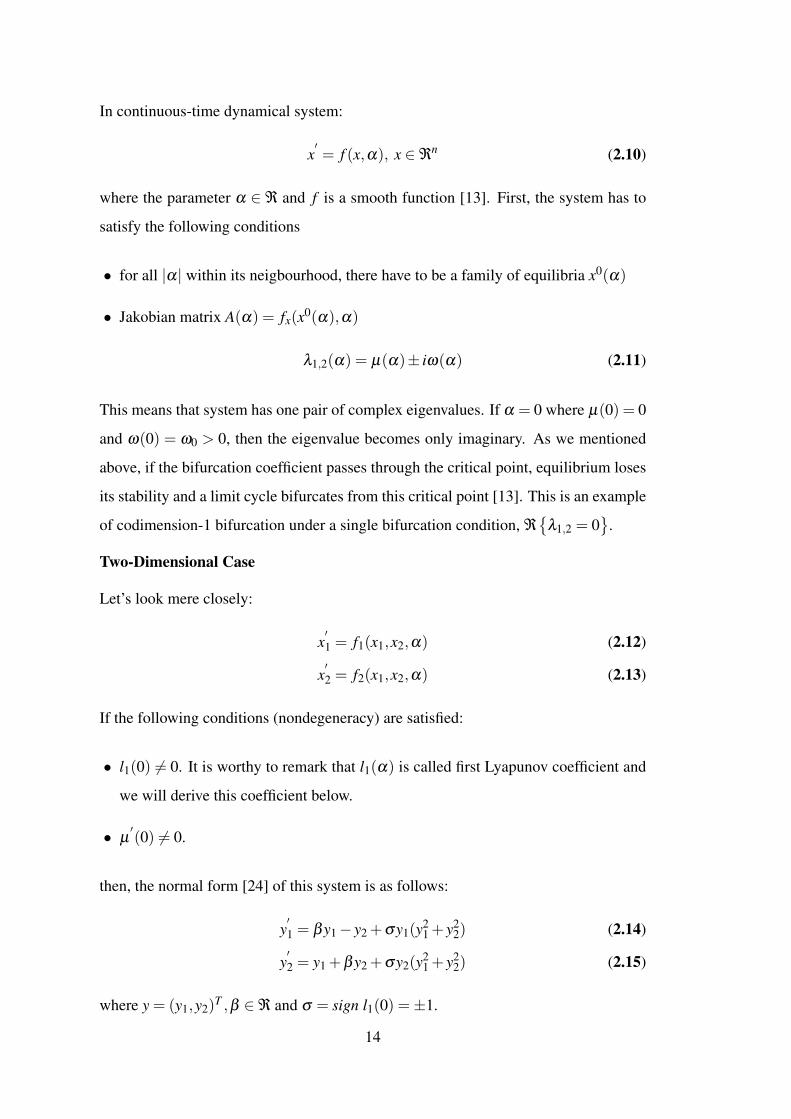
In continuous-time dynamical system:

x′= f (x,α), x ∈ℜ

n (2.10)

where the parameter α ∈ ℜ and f is a smooth function [13]. First, the system has to

satisfy the following conditions

• for all |α| within its neigbourhood, there have to be a family of equilibria x0(α)

• Jakobian matrix A(α) = fx(x0(α),α)

λ1,2(α) = µ(α)± iω(α) (2.11)

This means that system has one pair of complex eigenvalues. If α = 0 where µ(0) = 0

and ω(0) = ω0 > 0, then the eigenvalue becomes only imaginary. As we mentioned

above, if the bifurcation coefficient passes through the critical point, equilibrium loses

its stability and a limit cycle bifurcates from this critical point [13]. This is an example

of codimension-1 bifurcation under a single bifurcation condition, ℜ{

λ1,2 = 0}

.

Two-Dimensional Case

Let’s look mere closely:

x′1 = f1(x1,x2,α) (2.12)

x′2 = f2(x1,x2,α) (2.13)

If the following conditions (nondegeneracy) are satisfied:

• l1(0) 6= 0. It is worthy to remark that l1(α) is called first Lyapunov coefficient and

we will derive this coefficient below.

• µ′(0) 6= 0.

then, the normal form [24] of this system is as follows:

y′1 = βy1− y2 +σy1(y2

1 + y22) (2.14)

y′2 = y1 +βy2 +σy2(y2

1 + y22) (2.15)

where y = (y1,y2)T ,β ∈ℜ and σ = sign l1(0) =±1.

14

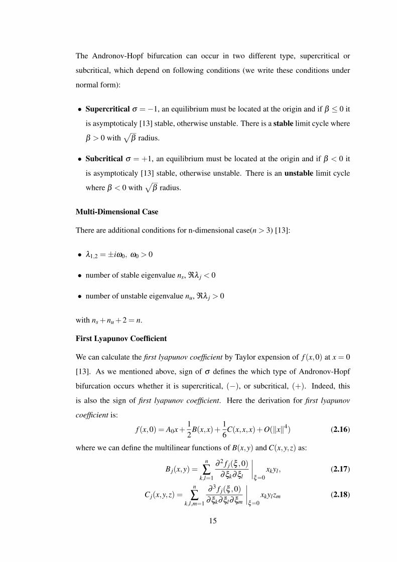
The Andronov-Hopf bifurcation can occur in two different type, supercritical or

subcritical, which depend on following conditions (we write these conditions under

normal form):

• Supercritical σ =−1, an equilibrium must be located at the origin and if β ≤ 0 it

is asymptoticaly [13] stable, otherwise unstable. There is a stable limit cycle where

β > 0 with√

β radius.

• Subcritical σ = +1, an equilibrium must be located at the origin and if β < 0 it

is asymptoticaly [13] stable, otherwise unstable. There is an unstable limit cycle

where β < 0 with√

β radius.

Multi-Dimensional Case

There are additional conditions for n-dimensional case(n > 3) [13]:

• λ1,2 =±iω0, ω0 > 0

• number of stable eigenvalue ns, ℜλ j < 0

• number of unstable eigenvalue nu, ℜλ j > 0

with ns +nu +2 = n.

First Lyapunov Coefficient

We can calculate the first lyapunov coefficient by Taylor expension of f (x,0) at x = 0

[13]. As we mentioned above, sign of σ defines the which type of Andronov-Hopf

bifurcation occurs whether it is supercritical, (−), or subcritical, (+). Indeed, this

is also the sign of first lyapunov coefficient. Here the derivation for first lyapunov

coefficient is:

f (x,0) = A0x+12

B(x,x)+16

C(x,x,x)+O(‖x‖4) (2.16)

where we can define the multilinear functions of B(x,y) and C(x,y,z) as:

B j(x,y) =n

∑k,l=1

∂ 2 f j(ξ ,0)∂ξk∂ξl

∣∣∣∣ξ=0

xkyl, (2.17)

C j(x,y,z) =n

∑k,l,m=1

∂ 3 f j(ξ ,0)∂ξk∂ξl∂ξm

∣∣∣∣ξ=0

xkylzm (2.18)

15

where j = 1,2...,n. Let q ∈ Cn, complex eigenvector of A0 ⇒ iω0 : A0q = iω0q and

for adjoint eigenvector p ∈ Cn : AT0 p = −iω0 p with 〈p,g〉 = 1. The first lyapunov

coefficient is:

l1(0)=1

2ω0Re[〈p,C(q,q, q)〉−2

⟨p,B(q,A−1

0 B(q, q))⟩+⟨

p,B(q(2iω0In−A0)−1B(q, q))

⟩]

(2.19)

Here we will also explain the bifurcation theory with discrete-time dynamical system

where we adress the computational model that we suggest.

2.2.2 Fold bifurcation (saddle node for maps)

In discrete-time dynamical systems (iterated maps), we can define the Fold bifurcation

(saddle-node for maps, limit point) in the generated map as a birth of two fixed

points (one stable the other unstable). Qualitative changes occur when the bifurcation

parameter passes through the bifurcation point (critical point). If the bifurcation

parameter reaches the critical point, system has an eigenvalue, λ = 1. This is

the general condition for Fold bifurcations in all dimensions [13]. Lets consider a

discrete-time dynamical system

x 7→ f (x,α), x ∈ℜn (2.20)

where α ∈ℜ and f is a smooth function. So,

• For α = 0 there exists a fixed point x0 = 0

• Jakobian matrix A0 = fx(0,0) with µ1 = 1

When the bifurcation point reaches the critical point, a fixed point bifurcates to two

different fixed points, one of them will be stable and the other one will be unstable. The

opposite of this situation can also be happen which means that a stable and unstable

fixed point collapses and only one stable fixed point occur. This phenemenon can be

seen in Figure 2.7

This is another example of codimension-1 bifurcation (µ1 = 1) where bifurcation

occurs in one-parameter sets of smooth maps. The literal conditions (nondegenerecy

16

Figure 2.7: Illustration of Fold Bifurcation.

conditions) for 1-dimensional case are as follows:

fx(0,0) = 1 (2.21)

α(0) =12

fxx(0,0) 6= 0 (2.22)

fα(0,0) 6= 0 (2.23)

To explain the quadratic coefficient, we consider the normal form for Fold bifurcation:

y 7→ β + y+σy2 (2.24)

where y ∈ℜ, β ∈ℜ and σ = sign α(0) =±1. In the normal form, if σβ > 0 there is

not any fixed points in the given system. In contrast, σβ < 0, system has one stable

and one unstable fixed point where y1,2 = ±√−σβ . At critical point, β = 0, there is

only one fixed point, y0 = 0,λ1 = 1.

Multi-Dimensional Case

There are additional conditions for n-dimensional case(n≥ 2):

• λ1 = 1

• number of stable eigenvalue ns,∣∣λ j∣∣< 1

• number of unstable eigenvalue nu,∣∣λ j∣∣> 1

with ns +nu +1 = n.

17

Quadratic Coefficients

The derivation of quadratic coefficient, α0, which is involved in the second

nondegenerancy conditions, and it can be calculated by Taylor expension as follows:

f (x,0) = A0x+12

B(x,x)+O(‖x‖3) (2.25)

where we can define the multilinear functions of B(x,y) as:

B j(x,y) =n

∑k,l=1

∂ 2 f j(ξ ,0)∂ξk∂ξl

∣∣∣∣ξ=0

xkyl, (2.26)

where j = 1,2...,n. Let q ∈ ℜn, critical eigenvector of A0 : A0q = q, 〈q,g〉 = 1 and

standart inner product 〈p,g〉= pT q with p ∈ℜn : AT0 p = p,〈p,g〉= 1. The quadratic

coefficient is:

α0 =12〈p,B(q,q)〉= 1

2d2

dτ2 〈p, f (τq,0)〉∣∣∣∣τ=0

(2.27)

18

3. SELECTING AN ACTION

When the brain collected input from more than one sensory modalities, it often

processes with high and accurate performance in one or more of the neural subsystems.

As there exists large sensory input from the environment, it is now accepted that

each data possible to distribute to relevant subsystems. In the presence of different

input modalities, it is claimed that making a decision is one of the tough processes in

the brain. Comprehensive information processing ability in brain provides making

a decision for availiable competitive actions by mediating related networks and

formations in brain. The studies in neuroscience literature show that the BG circuits

play key role in these formations [2, 10, 25].

The BG circuits are situated in the midbrain which means that this group of nuclei are

the ancient part of the mammalian brain [26] due to the selecting an appropriate action

is necessary for staying alive. In addition, from the point of evolutionary biology, BG

circuits can be claimed as a window of cerebral cortex. In BG, unilateral or reciprocal

connections exist through the cerebral cortex, cerebellum, thalamus, and other brain

regions. BG circuits are associated with in a wide range of brain functions, such as

perception, learning, memory forming, besides being effective in motor functions [2,

8, 10, 25, 27–30]. Their functions in cognitive processes as AS, GDB and selective

attention have been studied throughly in recent years [2, 3, 27, 31, 32].

Models of AS processes in BG range from conductance-based models, through spiking

neural networks, to system-level models [33]. Existence of at least five different loops

of cortex-basal ganglia-thalamus has been suggested in [10]. Each loop is assigned

different cognitive tasks but they have interconnection between each other, where

these connections are claimed to be designed in a spiral frame [34]. The principle

substructures of BG circuit are proposed to be comprised of input nuclei, Striatum (Str)

and Subthalamic Nucleus (STN), and output nuclei, Substantia Nigra pars Reticulate

(SNr) and Globus Pallidus internal (GPi). The major input station in BG is Str and this

19

subcortical area is divided into subsections where two DA receptors are must effective.

One of these receptors is D1 subtype and this regions project primarily to the output

nuclei of BG to inhibit them. These output nuclei SNr and GPi in turn inhibit the cortex

through Thalamus (Thl). This pathway is direct pathway:

Cortex (Excites) → Striatum−D1 (Inhibits) → Snr/Gpi (Inhibits) → T halamus

(Excites) → Cortex (Excites) → Brainstem

Whereas in the indirect pathway D2 receptors are effective and they have inhibitory

effect on Globus Pallidus external (GPe) to disinhibit STN through GPi. The indirect

pathway is:

Cortex (Excites) → Striatum−D2 (Inhibits) → Gpe (Inhibits) → ST N (Excites)

→ Snr/Gpi (Inhibits) → T halamus (Excites) → Cortex (Excites) → Brainstem

Based on these neurophysiological facts, many BG models now exist, all having

different approaches especially in explaining the correlation of direct and indirect

pathway. One approach considers the direct pathway as a main part of selection

mechanism and claims that indirect pathway antagonize the direct pathway by

suppressing unwanted movements [32, 35, 36]. To investigate these correlation in the

Str, direct pathway is added in the previous model in [7]. Here, to give an insight for

BG network, Figure 3.1 is given:

As we mentioned above, there are at least five different loops in BG for assigned

different cognitive tasks. Now, we will explain which loop of BG we consider and how

we modeled this loop by means of discrete-time dynamical system approach. The main

contribution of this work is to extend the model that proposed in [7] including the direct

and hyperdirect pathway to explain the DA effect on AS. The extended model helps

us to explain the BG circuit’s switchboard-like selection mechanism [2, 27] by using

nonlinear dynamical approach with the bifurcation analyses which will be discussed in

Chapter 4. Here, we will explain the model focusing on DA effect.

3.1 Modelling Action Selection

The sub-regions of neural system communicate with each other by interconnection

neurons and realize any process via neurotransmitters along neural pathways. To

20

Figure 3.1: Basal Ganglia Circuit.

understand the mechanism giving rise to cognitive processes, we have to consider the

neurotransmitter systems. As neurotransmitters have constitutive effect on cognitive

processes, DA release has a modification role in BG. Amongst eight different

dopaminergic pathway, nigrostriatal pathway modulates AS process in BG [37].

Striatonigral pathway (prefrontal loops in Basal Ganglia) is associated with motor

control and related to dopaminergic pathway [28]. Dysfunction of this pathway causes

disorders such as PD and HD [10, 38–40]. A proposed corticostriatal neural network

model by Amos [41] is achieved to investigate the mental disorders by using Wisconsin

Card Sort Test. The perseveration of Schizophrenic and Huntington’s patients are

demonstrated and suggested that the problem is caused due to unsystematic errors of

matching in the Str where the DA modification is well-known today.

Besides different brain areas that produce DA, one of the transmission of DA starts

from Substantia Nigra pars Compacta (SNc) through the Str. These regions are the

part of the basal ganglia-thalamus-cortex circuits [10]. Retrograde and anterograde

tracing studies have shown that the basal ganglia-thalamus-cortex circuits and a.k.a.

21

striatonigrostrital pathways have important role in AS and learning phenomena, as

we mentioned above. There are a number of computational models evaluating

the neurophysiologic work on BG and related neural substrates taking part in AS

[2, 5, 7–9, 32, 33]. and also some others where cognitive processes are investigated

considering the robot models [42, 43]. The cortico-striato-thalamic model considered

in this work for implementation of GDB is based on these neurophysiological facts and

is capable to explain how primates make appropriate choices and learn associations

between environmental stimuli and proper actions [7].

In [10], different regions of BG are considered for different neural circuits, but

principle substructures are proposed to be Str, STN, GPi and GPe, SNr and SNc. Due

to the reason that the relationship between these substructures, for example cortex and

Thl is very complex, the model used in this work consider only a subgroup of these

relations which are important for action selection, so it is simpler. The connections

considered in the model are illustrated in Figure 3.1. A part of this computational

model of AS, where only indirect pathway is considered, has been shown to realize a

sequence learning task [7]. Here, we have been extended the model in [7] by including

direct and hyperdirect pathway to mimic the modulatory effect of DA release on Str.

We aim to model the modulatory effect of DA on AS with a computational model

which can establish sufficient functionality to exhibit relevant behaviour in embodied

robotics. The computational model has been developed at the system level [7] as in

the well-known work of Prescott et. al. [42]. In [42], saliencies that exist in a tight

competition effectively switch the behaviour of the computational BG model realizing

the AS mechanism in the embodied architecture. The saliencies which control the

behavior of the mobile robot are generated in the motivational and sensory sub-systems

as a priori coefficients in [42]. Although the work in [42] is important as it shows that

the biologically plausible models of the BG can be used for the control of physical

devices, it is only a first step as it lacks the ability of determining saliencies by a

learning process. We focus especially on this aspect and proposed a model [7] capable

of generating an adaptive process where the parameters of the model modify the

behaviour of BG circuit taking part in AS. In order to make the model functional and

realize it in embodied robotics’ task, the neural substructures, that are related to the

22

BG circuit we consider, are discussed as a mass model. Furthermore, each neural

substructure acts according to the tangent hyperbolic function, f (.):

f (x) = 0.5(tanh(3(x−0.45))+1) (3.1)

Since the output of the neuronal activity can be defined as an all or none, we used the

tangent hyperbolic function to fulfill these phenomenon, see Figure 3.2. Based on the

Figure 3.2: Tangent hyperbolic function.

discussion as mentioned above, a representation of BG circuit with its connection to

related neural substructures are started with Cortex the following difference equations:

S(k) =WcI(k) (3.2)

Ctx(k+1) = f (λCtx(k)+T hl(k)+S(k)) (3.3)

The input substructure of the model is Cortex which transmits the sensory data to the

Str, Thl and STN. The main effect on cortex is due to excitatory signal from Thl which

corresponds to the result of selection process. It is worthy remark that the variables Ctx

and T hl stand for vectors corresponding to cortex and Thl constituents of prefrontal

loop in BG, respectively. The dimensions of these vectors are determined by the

number of actions to be selected, in this case, the vectors belong to ℜ3 as there are

three actions to be selected that we consider in our robot task. S(k) constitutes the

salience matrice, and Wc matrice that we call efficiency of sensory input, I(k), denotes

the parameters which impress the environmental senses. Wc is the main bifurcation

parameter in our system, we will discuss it in Chapter 4. An action is selected, when

23

the value of one of the cortex variable becomes almost one. This corresponds to firing

of related neural structure, as we mentioned above.

The interconnections between substructures Str, GPe, STN and SNr/GPi, that are

respectively denoted by Str, GPe, Stn, GPi are modelled with same approach as

follows:

Str(k+1) =Wr f (Ctx(k)) (3.4)

GPe(k+1) = f (−Str(k)) (3.5)

Stn(k+1) = f (Ctx(k)−GPe(k)) (3.6)

GPi(k+1) =Wd f (Stn(k)−Str(k)) (3.7)

T hl(k+1) = f (Ctx(k)−Gpi(k)) (3.8)

There are two more bifurcation parameters in the model where Wr denotes the effect

of DA release on Str and Wd denotes the correlation between the direct and indirect

pathways in the circuit. These parameters are effective in selection mechanism, so

bifurcation analysis, considering these coefficients, will be given in Chapter 4.

To show the model is capable selecting an action, as give in Figure 3.3. Since the output

of the system corresponds to Ctx component, each dots represent one of which cortex

variable is firing at the given input . Axises denote the values of three components

of salience matrice, respectively. This figure is obtained by solving the Equation

3.2-3.8 in-house MATLAB with initial conditions are generated randomly. When there

exist three actions to be selected, three dimensional salience-space comprises different

subspaces where Wc, Wr and Wd reshapes this space. As the DA release has a key role

in AS, we will show its effect on the computational model of BG. Once we select a

priori coefficients which means that a basal DA release exists in the BG, a classification

of three subregions are obtained.

In Figure 3.3a there are subregions of salience-space where only one of each salience

determine the action to be selected. This means, model selects an appropriate action

if the relative salience value is in one of these regions. In Figure 3.3b, two salience

combinations out of three determine the action to be selected. The all or none selection

regions is given in Figure 3.3c.

24

Figure 3.3: Wc = 0.8, Wr = 0.3 and Wd = 1. Legend of the colors; green: first salience,red: second salience, blue: third salience, magenta: first-second salience,yellow: first-third salience, cyan: second-third salience, black: all-selectedsalience, grey: non-selected salience, respectively. Legend is same as inFigure 3.4 and 3.5.

3.2 Related Diseases

Deficit or excessive level of DA in the D1 and D2 receptors in Str causes several

behavioral disorders, such as PD and HD [10,38–40]. The direct and indirect pathway

have an antagonistic functions in BG and DA modulates them. D1 type DA receptors

are effective in direct pathway where DA excites the inhibitory effects of Str in

Gpi/SNr. This means that Str inhibits Gpi/SNr, so Gpi/SNr activity is decreased and

in turn Thl activity is increased which causes a disinhibition in motor activity (one of

the possible action selection). On the other hand, D2 type DA receptors are situated in

indirect pathway. If the DA release increases then there would be less activity in GPe

through Str. Less indirect pathway activity means again increased motor activity. If the

balance of the direct and indirect pathway breaks, selecting an action process becomes

easy or difficult for body which points out the important behavioural disorders.

The model that we propose can be further used to establish a framework for

understanding the cause of physiological diseases related with BG circuits. Based on

the bifurcation analysis that we will explain in Chapter 4, the proposed model provides

us results to discuss these disorders. With bifurcation analysis, the proposed model

shows that the DA effects on the Str causes the transition of the salience-space. The

25

transition of parameter demonstrates that there is an association between subcortical

dysfunctions and DA effects on Str in BG circuit. These simulation results are

consistent with neurophysiological experiments [10, 38–40].

It is now accepted that loss of dopaminergic neurons in SNc induces the dysfuntion on

Str which causes less activity in direct pathway, in contrast more activity in indirect

pathway [38]. As the level of the DA has a role in different physiological disorders, it

is well-known that loss of DA level in BG circuit causes PD which means difficulty in

accomplishing an action as in Figure 3.4. As it is followed from Figure 3.4c, selecting

an action became more difficult (increased black dots).

Figure 3.4: Wc = 0.8, Wr = 0.1 and Wd = 1.

HD is another neurophysiological disorder which is related with BG circuit [39, 40].

The key sypmtoms of HD are difficulty in muscle coordination, excessive motor

behaviours and cognitive decline with psychiatric issues. HD typically causes an

abnormal involuntary movements, difficulty in initiating appropriate actions and

inhibiting inappropriate actions, which is the first step of this disorder and is called

with chorea [39]. In addition, HD has several impact on cognitive abilities such as

planning, cognitive flexibility and rule acquisition [40].

Even how the BG damage causes the HD is not fully understood, it is now accepted

that excessive DA level in BG circuit has role in HD which means choosing more than

one action at a time, as it can be seen in Figure 3.5. In contrast with Figure 3.4c,

selecting an action become very easy (increased grey dots in Figure 3.5c).

26

Figure 3.5: Wc = 0.8, Wr = 0.8 and Wd = 1.

So, to avoid this undecisive situations, RL has been implemented to the model and

once the learning is completed, system selects the right decision at the right time in

all circumstances. We will continue to explain the learning architecture in proposed

model next chapter.

27

4. LEARNING TO SELECT AN ACTION

Goal-Directed behaviour comprises two different concepts; Action Selection and

Learning as mentioned above. For many years, neuroscientists were strictly thinking

that BG circuits have role in motor behaviour control only. The motivation of this

approach was based on the motor control damaged patients who have certain symptoms

in their BG substructures [44]. However, recently, there are different works showing

the role of BG in different cognitive and emotional functioning such as reward related

learning, habit forming, GDB and RL [45, 46]. In this chapter, we will focus on how

we constitute the learning and AS together based on the structures of the BG circuits

and we will suggest an algorithm to explain the GDB in primates.

The main focus of our approach is to bring the dorsal loop of Cortico-Striato-Thalamic

circuits and TDL together. The reason that we use TDL is there are works relating

learning process in the brain with temporal difference, especially in BG circuit

[1, 4]. Indeed, due to the reason that recent studies show the learning in BG is

somehow exactly same as RL, we considered the TDL in constituting the GDB [1].

The interaction between the different loops in BG take part in different cognitive

functions beside motor control. Also effect of dopaminergic modifications on learning

is well-known in neuroscience literature nowadays [1, 47, 48]. So, we especially

focused on the DA effect in Str during the modelling process by means of bifurcation

theory. Since the main aim of this work is to adress the relationships between AS

and RL, TDL has been implemented into the model considering these bifurcation

analysis. As the model is expected to find correct (appropriate) choice after learning is

accomplished, we investigate the model by considering the Bifurcation Theory before

the implementation of TDL.

For more than fifteen years, nonlinear dynamical systems have been important part of

neurocomputational modelling and have consistently became a common tool for the

computational neuroscientists to explain the networks in brain. Nonlinear dynamical

29

system approach for modeling the neural structures gives us the possibility to control

the system with bifurcation parameters. After obtaining the whole architecture of the

model’s behaviour by means of the bifurcation analysis, we implemented the RL into

the model. Therefore, in this work, we considered the neurocomputational model

of BG Circuit with bifurcation theory and RL together, and suggested an algorithm

to constitute the learning architecture. We explain the switchboard like mechanism

[2, 27] in BG Circuit with Fold Bifurcation (FB). This investigation confirmed that

the given model can be modified to obtain appropriate behaviour if it satisfies FB

conditions. To realize this modification, RL is utilized and with RL the parameters

of the system corresponding to bifurcation parameters are updated to model learning

to select appropriate actions in an unfamiliar environment. Thus, first, the bifurcation

analysis will be completed based on different bifurcation parameters, then the TDL

will be explained with further details. Finally, we will conclude this chapter with how

bifurcation analysis and RL are brought the idea of the selection process in BG circuits.

4.1 Bifurcation Analysis

Neurocomputational model for AS circuit given with Equation 3.4-3.8 is investigated

using bifurcation analysis and this investigation confirmed that the given model

can be modified to obtain appropriate behaviour. Here, we will start to explain

the bifurcation analysis with the one parameter bifurcations, then we will use

two-parameter bifurcation analysis to explain the structure of the model.

4.1.1 One-Parameter bifurcation analysis

First of all, we used the one parameter bifurcation analysis of the system given in

Equation 3.4-3.8 according to parameter Wc in neurocomputational model of BG

circuit, here we found FB (the explanation of FB can be found in Section 2.2) in this

system. In the context of AS, system has to be able to select an action depending on

initial conditions or saliencies. Besides there may exist two or more than two actions

to be selected, we use FB to explain the structure of this selection process. Due to two

different fixed points existing in the system at the same time, one of them corresponds

to the "not to choose" the choice and in contrast, the other one corresponds to "choose".

30

Starting these analysis with different parameter values have a role to change the

bifurcation points and it is obvious that also this continuation allows us to explain

the different fixed points locations. We will use this property in the system to explain

the AS process in the context of the given task which can be found in Section 5. The

model satisfies the fold (saddle-node, tangent) bifurcation conditions (see Section 2.2)

where one stable and one unstable fixed points exist in the generated map even may

be at the same time or different locations. The location of the different stable fixed

points depend on parameter values. In the critical points which are FB points, one of

the fixed point disappears and may be at the same time or with some delay another

fixed point borns. As we mentioned above, we can reshape the bifurcation diagram

with using different parameter values. First, we will investigate that the system given

in Equation 1 undergoes one FB, this means the second unstable fixed point borns after

the first fixed point disappears and then the unstable one disappears during the second

stable one borns, consecutively and this explanation gives rise to the switchboard like

mechanism in AS circuit. The bifurcation diagram can be found in Figure 4.1 with

eigenvalues during the bifurcation parameter is iterated.

Figure 4.1: a. The circles denote the unstable fixed point, dots denote the stable ones.System has two different stable fixed points with different locations. Oneof them corresponds to not-selecting an action (near “0”), the other onecorreponds to selecting an action (near “1”). b. Change of value of theeigenvalues with parameter Wc. There one eigenvalue is fixed at “1”, threeones are “<1” and two ones are “>1” in FB point.

31

As it can be followed in the Figure 4.1, in the generated map, system have different

stable fixed points which describe to select and not to select an action, respectively.

There exist one stable fixed point which is near “0” and then it disappears and later

reappears around “1” while the bifurcation parameter Wc ∈ [0,1]. As the bifurcation

parameter reaches FB when Wc=0.21, the unstable fixed point collapses with stable

one and disappears while another stable fixed point around “0.98” borns. Thus there

exist a region where unstable fixed point is observed.

At the critical point where bifurcation parameter Wc=0.21, the eigenvalue conditions

of being outside the unit circle for unstable and being inside the unit circle for stable

case are satisfied as it can be seen in Figure 4.1. The stable fixed point near “0” means

that system cannot select an action, on the other hand the stable fixed point at “0.98”

means that the system selects an action. Even though we expect to see two stable fixed

points, there exists only one.

As we mentioned below, we can reshape this bifurcation diagram using different

parameter values. We will use this approach to explain the significant situation in the

given task, see Section 5. Here, the system has two different FB at different locations

as it can be seen in Figure 4.2. The parameter values can be seen in both Figure

4.1 and 4.2. The difference betweens two maps are; first the FB numbers and then

the bi-stable phase portrait occurs in the second situation. We can see the two FB

with following the eigenvalues in Figure 4.2. Between the two FB, following system

satisfies the eigenvalue conditions for FB. We can give more precise knowledge about

this situation; in Figure 4.1b black circles which show the first conditions of FB (see

Section 2.2) start to reach “1” during the second stable fixed points birth not the process

of the first stable fixed point disappear, and this means system has only one FB during

the second stable fixed point birth because the conditions of FB. On the other hand,

same as the explanation in first case, one of the eigenvalue, which is denoted by black

circles in Figure 4.2b, fixed at “1” while the process of first unstable-stable fixed points

collapse and the second stable-unstable fixed points collapse.

It is worthy to remark that between the significant bifurcation parameter values (Wc ∈

[−0.22,0.403]), there exist two stable fixed points at the same bifurcation parameter

value. This situation allows us to use these two different fixed points for different

32

Figure 4.2: Demostrations are same as in Figure 4.1 a. System has two different stablefixed points between the two FB. One of them corresponds to not-selectingan action (near “0”), the other one correponds to selecting an action (near“1”). In this situation, system has a bi-stable phase portrait which isrepresented by FB. b. Change of value of the eigenvalues with parameterWc. As it can be followed in Figure 4.1b, FB conditions are satisfiedbetween two Bifurcation points, see Section 2.2.

tasks as it will be explained in Section 5. Around the bifurcation point there are two

domains of fixed points between “-0.22” and “0.403”. When we fix the parameters

in this region, the proposed model decides to select/or not select an action depending

on the initial conditions. This explains how the system given by Equation 3.4-3.8

accomplishes AS according to the input value Wc. So to observe the effect of input

value Wc while changing Wr, another example can be found in Figure 4.3.

Before start the explanation about two bifurcation analysis, we want to show the

significant paramater values effect on system’s behaviour as the modification of Wr

can also change the dynamic behaviour of the system. As shown in Figure 4.3, in the

beginning, system has only one fixed point but there is a region where non-convergent

solutions (quasi-periodic) began and changing the value of the parameter further causes

system to settle down at another fixed point. The quasi-periodic behavior corresponds

to the case where search is carried, so the dynamic systems behavior is not settled to

a fixed point. As it can be seen in Figure 4.3, the other bifurcation parameter (in this

case, Wr) has a role in changing the dynamic behaviour of the system. So, we will

33

Figure 4.3: One parameter bifurcation diagram according to the Wr with the parameterof Wc = 0.2.

continue to explain the dynamic behaviour of the system with using two-parameter

bifurcation analysis.

4.1.2 Two-Parameter bifurcation analysis

We aim to model the modulatory effect of DA on AS with a computational model

which can establish sufficient functionality to exhibit relevant behaviour in embodied

robotics. As it is explained in Section 3.1, Wr corresponds to the DA effect on

Str and Wd the correlation between the direct and indirect pathways in the circuit.

These parameters are effective in selection mechanism, so bifurcation analysis with

considering these coefficients is important to constitute the learning algorithm in

the model. To observe the effect of input value Wc while changing Wr, the two

parameter bifurcation diagram given in Fig. 4.4 is obtained. Here while Wr < 0.23 and

Wc ∈ [0,1] there is one stable fixed point and while keeping Wc ∈ [0,1] but changing

Wr ∈ [0.23,0.51] non convergent solutions (quasi-periodic) begin till another stable

fixed point appears. This quasi-periodic solutions mean that system cannot decide

which action to select. How the system’s salience-space is rehaped can be explained

with this bifurcation analysis. As it can be seen in Figure 3.3-3.5, with different

parameter values, different salience-space configuration is formed. The ability of the

system to select an action is increased or decreased with these parameters. Based on

34

Figure 4.4: Two parameter bifurcation diagram for Wr and Wc.

the discussion in Section 3, DA release on Str has a significant role to explain the

selection process in brain. This analysis explains the DA effect on Str: when the

stable fixed point is located around “0” even the input value is high enough, system

cannot select an action (This is shown in Figure 3.4, where the area of the selection is

decreased in Figure 3.4a, and the non-selection area is increased in Figure 3.4c) where

the DA level is less to select a desired action. On the other hand when the DA release

is increased, system selects the action in all circumstances which corresponds to HD

(This is shown in Figure 3.5, where the area of the selection is increased in Figure 3.5c,

and the non-selection area is dicreased in Figure 3.5c).

There exists another bifurcation parameter, Wd , which corresponds to correlation of

the direct and indirect pathways in the BG circuit. The bifurcation analysis for Wd

shows that the model’s behaviour becomes unstable when Wd ∈ [0.67,0.75] (Figure

4.5). If this connection increases constantly, system possibly selects an undesired

action and it means that indirect pathway cannot antogonizes the direct pathway to

select an appropriate action.

4.2 Reinforcement Learning

Reinforcement learning is a learning formation with respect to the interaction between

agent and environment [49]. Based on this interaction, agents make the appropriate

decisions by evaluating the consequences of these decisions. These evaluations

depend on different perspectives such as; past experiences, new conditions or

35

Figure 4.5: Two parameter bifurcation diagram for Wd and Wc.

reward/punishment expectations. The main architecture of RL depends on trial/error

learning with essential reward predictions [4, 31]. In RL, the ultimate goal is to

reach the minimization of the error in expectation through the maximization of value

for reward which are calculated over time. The evaluation to find the appropriate

output of network in RL depends on value assignment about given situation with

reward/punishment formation rather than consider by any teacher’s assessments. The

basic definition of RL can be given with reward/punishment formation in which the

network is matched the association between reward/punishment and stimuli/actions.

Each action, agents decide, creates a reinforcement by means of particular situation and

this is explicitly a result of unsupervised learning: not from a teacher’s assessments,

from the basis of reinforcement they receive themselves.

The experimental studies on animals, psychologists have focused on more than a

century have an important impact in constitution of TDL framework. The studies

on the TDL theory have been started with Rescorla-Wagner where the Pavlovian

conditioning is considered adressing the correlation of learning theme and associative

stimulus [50]. Most of studies starting with this theory point the explanation of how

human brain evaluates the error prediction. In comtemporary neuroscience, as many

studies have suggested [31, 51], the midbrain, significantly nigrostriatal DA pathways,

is the adress of these learning phenomena. We can claim that TDL is a learning

framework where the Pavlovian conditioning experiments is the base of it. There exist

different studies both in experimental and computational neuroscience to understand

36

the DA release and its effect on significant brain networks and these studies point out

the reward related learning and also drug addiction [1, 11]. This is the reason why

we have been used TDL within computational model of AS circuit. Besides different

disciplines considering RL for the problems they deal with, the principle case that we

are interested in RL is Machine-Learning. We can summarize the framework of TDL

in Machine-Learning with two discriptions: Actor-Critics and Q-Learning [49].

We have been focused on neural circuits with the aspect of mathematical and

computational models, where we deal with how we can explain the learning

mechanism with unsupervised learning approaches. The main focus of our work

is inherented in RL, particularly in TDL. We have defined the AS as making

an appropriate decision at the right time, see Section 3.1. Facing with rewards

or punishment can cause significant effects on decision-making which means the

appropriate actions depend on the adaptation of the conditional changes in existing

environment. The ultimate goal of our work by which the reward or punishment

has a role to make an appropriate decision is to represent the neural formation of

learning. The TDL we use to handle with finding the appropriate decision is based

on neurobiological and psychological experiments, as mentioned above. In addition,

this approach can give an insight of modification process in synapsis [52].

We will discuss the process of TDL within our study. So, we will start to explain

the learning process of the salience differences which depends on the adaptation of

the efficiency of sensory input matrix, Wc. Then, we will continue with sequential

learning where we thereafter consider the DA effect on Str, Wr. Before concluding this

chapter, the whole architecture of the learning process in our work will be given with

pseudocode that we have been suggested. We have been simulated the model with

TDL in MATLAB before implementing on the robot.

4.2.1 Adaptation of the efficiency of sensory input

The parameters of the dynamical system corresponding to neurotransmitters are

modified with TDL. Here, we will explain the efficiency of sensory input (Wc)

adaptation through TDL to determine the proper action. To modulate the AS circuit

37

(see Section 3.1), the adaptation equations start with as follows:

Wc =Wc +ηcδ (k)c f (ctx(k))S(k) (4.1)

Here, the learning rate ηc = 0.2, δ denotes the error in expectation, f (ctx(k))

represents the output value of the AS circuit and S(k) represents the multiplication

of input value, I(k), and efficiency of this input value, Wc.

The reward function is determined by using AS circuit’s output. If the system find the

desired action, this function is set to “1” for reward otherwise “-1” for punishment.

Then, system evaluates the error in expectation with following equations same as

traditional TDL:

δc(k) = rc +µVc(k+1)−Vc(k) (4.2)

Error in expectation δ depends on the value assigner which is attained to the selected

action and future expectation with reward or punishment. The step size of learning

depends on discount factor, µ . The generated expectation value is based on value

assigner of the action which is also updated as follows:

Vc(k) =Wvc(k)S(k) (4.3)

Vc(k+1) =Vc(k)+µcδc(k)S(k) (4.4)

Once the saliencies are established, the AS circuit determines an action. This selected

action and the reward obtained for it interacts with the learning and the selection

process in AS restarts at each time step. The simulation results of the adaptation

process for efficiency of sensory input, Wc, can be seen in Figure 4.6. As it can be

seen in Figure 4.6, error in expectation converges the zero when the reward function is

“1” , otherwise the error in expectation diverges the zero. Once the error in expectation

reaches approximately “0”, Wc (efficiency of sensory input) is fixed at the (Wc=0.5).

This final Wc value corresponds to the significant meaning for our system’s behaviour.

As it can be seen in Figure 4.1.a, if the Wc value is bigger than the bifurcation point,

system has only one fixed point to determine the action to be selected.

After this learning process, system is able to distinguish the differences between the

actions to be selected. In order to compare the learning effect on AS process, the

38

Figure 4.6: Temporal difference learning process for Wc.

efficiency of sensory input matrices for beginning and for after learning process is

given as following:

W beginningc =

0.1 0 00 0.1 00 0 0.1

,W a f terc =

0.5235 0.1314 0.02250.0233 0.5311 0.02230.0236 0.1316 0.5226

(4.5)

The differences between each matrices show that the value on the diagonal of Wc are

set up the latter of FB point (Figure 4.1). There less significant changes occur rest of

the matrices’ components but these modificition can be omitted due to the system’s

architecture as mentioned in Section 2.1.

As it can be followed in Figure 4.6, system evaluates an error in expectation every

step time which depends on reward/punishment value. The difference between the

error in expectation in each step time is the result of the differences between the

reward/punishment and expectations. If the expectation of the value assigner is not

similar to the given reward or punishment, system evaluates significantly bigger error.

4.2.2 Adaptation of dopamine effect on striatum

We have extended the learning process in AS circuit by adapting parameter Wr which

corresponds to DA effect on Str. The main reason of this learning process is to

mimic the modulatory effect of this neurotransmitter in BG circuit. Based on the

bifurcation diagrams for the Wc and Wr parameters (see Section 4.1), we are able

to explain not only the importance of DA on determining the saliencies but also

39

differences between each salience circumstances. The ability of the system to decide

the action’s importance can be controlled with DA parameter, Wr. The bifurcation

analysis and learning idea depend on the DA effect on learning process, whereas the

psychological experimental results show the importance of this neurotransmitter in

primate’s brain. The modification of the Wr parameter starts once the TDL for Wc

parameter is accomplished. The TDL equations for Wr parameter is similar to the

modulation of Wc parameter with certain differences. The equation for the modification

of Wr parameter as follows:

Wr =Wr +ηrδr(k) f (Ctx(k))Str(k) (4.6)

where ηr denotes discount factor, Str(k) denotes Str as mentioned in Section 2.1. The

error in expectation:

δr(k) = rr +µrVr(k+1)−Vr(k) (4.7)

where µr = 0.2 in this case. The value assigner equations are:

Vr(k) =Wvr(k)Str(k) (4.8)

Vr(k+1) =Vr(k)+µrδr(k) f (Ctx(k)) (4.9)

Once the TDL process for Wr is accomplished, system is able to decide the importance

of each action. It is worthy to remark that learning process of Wc is important for

the competition of saliencies between each other, in contrast after the learning process

of Wr, system focuses on each saliencies respectively and understand the importance

of them. The differences between the beginning and after learning for Wr for each

salincies can be found as follows:

W beginningr =

[0.0560 0.0613 0.0301

],W a f ter

r =[0.8559 0.7641 0.7540

](4.10)

The simulation result of TDL for Wr parameter can be seen in Figure 4.7.

The concepts of this learning process is same as the learning for Wc. Once the learning

is accomplished, the error in expectation converges “0” where these errors depend on

the reward/punishment value. In Figure 4.7, it can be seen that the Wr=0.8 which is

the desired value due to the our main aim as discussed in Section 4.1. In this case,

40

Figure 4.7: Temporal difference learning process for Wr.

system has two different fixed points at the same time, so system is able to decide to

which fixed points based on the importances of occuring case (see Figure 4.2).

4.2.3 Proposed method

The algorithm we have been proposed for learning is constituted from bifurcation

analysis both in one-parameter and two-parameter through TDL for Wr and Wc

parameter, as explained above. Considering these two concepts together helps us

to propose an approach to understand how primates make appropriate choices under

different circumstances. It seems intuitively obvious that exploration of a new maze

would lead to be a first step of our method to be tested.

41

Algorithm 1 Calculate Wc and Wr

Require: These codes work on Webots 6.0.0 and all of the pseudecodes are given withC Programming Synopsis.

Ensure: You should include the related library at the beginning of your codes, such asif you want to use the distance sensors you should call the distance sensors library.

Require: 0 <Wc < 1∧Wd < 0.67Ensure: µ = fx(0,0) = 1∀|µstable|< 1∧∀|µunstable|> 1nstable +nunstable +1 = ns⇐WcIwhile Error > |0.04| do

for ( do i=0;i<51;i++)p (MotorCortex)

p1..3[i+1] = L_ f unc(lambda2∗ p1..3[i]+m1..3[i]+ s1..3)m (T halamus)

m1..3[i+1] = L_ f unc(p1..3[i]−d1..3[i])r (striatum)

r1..3[i+1] =Wr1..3∗L_ f unc(p1..3[i])e (GlobusPallidusExternal)

e1..3[i+1] = L_ f unc(−r1..3[i])n (SubthalamicNuclues)

n1..3[i+1] = L_ f unc(p1..3[i]− e1..3[i])d (GlobusPallidusInternal)

d1..3[i+1] = L_ f unc(Wd ∗n1..3[i]− r1..3[i])

end forN⇐Ctx(k)if N < 0.85 then

Rewardc⇐ 1else

Rewardc⇐−1end ifValuec(:,kk+1)⇐ valc ∗ I′

Errorc(:,kk)⇐ Rewardc + γc ∗Valuec(:,kk+1)−Valuec(:,kk)valc⇐ valc +nuc ∗Errorc(:,kk)∗S(k)Wc⇐Wc +nuc ∗ [Errorc(:,kk)]′ ∗Wc.∗ f (N).∗S(k)if Wc > 0.403 then

Rewardr⇐−1else

Rewardr⇐ 1end ifValuer(:,kk+1)⇐ valr ∗Str(:,k)Errorr(:,kk)⇐ Rewardr + γr ∗Valuer(:,kk+1)−Valuer(:,kk)valr⇐ valr +nur ∗Errorr(:,kk)∗ f (N)Wr⇐Wr +nur ∗ [Errorr(:,kk)]′ ∗Wr.∗ f (N)∗Str(:,k)kk⇐ kk+1

end while

42

5. AN APPLICATION: FORAGING TASK

In order to explain the efficiency of brain-inspired computational model summarized

in Chapter 4 and investigated in Chapter 5, we have been tested our model on robotic

application which is considered in cognitive robotics’ topics. In the framework

of cognitive robotics, the principle aim is to model the animal’s cognition while

information processing in robot mimics the formations of brain as opposed to Artificial

Intelligence approaches [53, 54]. The cognitive robotics applications have capability

to demostrate a wide range of brain formations, such as processing of perception,

attention, planning, motor behaviours and perhaps even about their instrinsic states

[42, 43, 53]. Recently, the applications of these cognitive processes have been

increased throughly in computational neuroscience since the autonomous devices

became important for medicine devices or elder services.

In cognitive robotics, the interaction between the agents and environment is the

challenging step that has to be solved. On the contrary of usual artificial intelligence

algorithms, specifically supervised learning, brain-inspired mathematical models

embody the unsupervised learning while mimicking the information processing in

brain. Since the ultimate goal of cognitive robotics is creating an intelligent agent

which act in the real world, brain-inspired computational models have a capability to

demostrate the sensation, action selection and motor behaviour at the same time. The

computational model that we suggested above serves to demonstrate these abilities

under competitive situations.

For more than ten years, cognitive robotics applications have been studied to explain

the cognition processes in brain where the neural substructures and the connections

between them are considered [42, 53, 54]. In the well-known work of Prescott et.al.

[42] a robot model for action selection is given in the embodied architecture. This

robot model mimics the behaviour of a rat in an unfamiliar environment and it is

based on mathematical model of basal ganglia which is inspired by neurophysiologic

43

studies [2, 8]. In [42], saliencies that exist in a tight competition effectively switch

the behaviour of the computational BG model realizing the AS mechanism in the

embodied architecture. The saliencies which control the behavior of the mobile robot

are generated in the motivational and sensory sub-systems as a priori cofficients in [42].

Although the work in [42] is important as it shows that the biologically plausible

models of the BG can be used for the control of physical devices, it is only a first

step as it lacks the ability of determining saliencies by a learning process. In this

thesis, we focused especially on this aspect and extended the proposed model [7] which

capable of generating an adaptive process where the parameters of the model modify

the behaviour of BG circuit taking part in AS.

In this thesis, the idea is to accustom the work in [42], and develop it further by

implementing reinforcement learning to determine the saliencies which influence the

choice of the rat. Thus, it is shown that robot implementation of neural circuits which

are capable of realizing reinforcement learning is possible. It has to be emphasized that

a more complex cognitive process than action selection, i.e., goal-directed behavior

is implemented on a mobile robot, Khepera II. It is shown that basal ganglia take

part in selecting an action amongst different choices based on the saliencies of each

possibility. It is worthy to remark that again, the process of learning has not been

considered in [42], where the choices depend only on a priori saliencies where

they need busy signals to avoid the inconvenience situations. So the saliencies

are reconsidered and priority of one over the other is determined according to the

environmental conditions with reinforcement learning. It is shown that a simpler model

of the cortico-striato-thalamic circuit considered for action selection can fulfill the

expected behaviour based on these saliencies. Thus, the improvement of this work

over [42], is the utilization of reinforcement learning to determine the choices and

this is provided by using a simpler model of cortico- striato-thalamic circuit for action

selection [7].

In this chapter, we present the fundamental concepts about the task that we solved.

Then, the description of the whole architecture of the model and the experiments that

show the differences between the a priori situation and learning process. After that, we

will continue to explain the simulation results for the implementation of the proposed

44

model on the mobile robot Kheperea II. Before concluding, the dopamine effect on the

learning process will be given.

5.1 The Task and Environment

The task of the robot is inspired from [42] where the robot mimics the behaviour of a

rat’s search for food in an unfamiliar environment. The action selection task that we

considered in this thesis based on this scenario depends on three saliencies which are

search-detection, pick up-carry the food and return to the nest. We have been extended

the task suggested in [42]. The task is planned such that as the feeling of fear ceases,

the rat begins to search for food and during random search, learns to recognize food

supplies and picks up the food and carries it to the nest. In an unfamiliar environment

the rat’s first feeling is to fear and action choice is not to move, but sometime later their

need for food becomes irresistible and they begin to feel hunger. As time goes by, they

start to feel more confident and the feeling of fear ceases. These two feelings, fear and

hunger are intrinsic processes for the rats. Hunger depends on time and fear depends

on environmental conditions which may be the existence of lights, foreign animals

or noises. The differences between the sensory systems of the mobile robots and the

rat have to be resolved in order to mimic the behavior of a rat. In rat’s, the central

nervous system is responsible in recognizing the food and differentiating it from other

objects. They use their eyes and/or olfactories while mobile robots use the distance or

light sensors to recognize the objects. Khepera II has eight different light and distance

sensors, the location of these sensors and also the obstacle, light location and potential

food can be seen in Figure 5.1.

In our context, at the beginning of the experiment reinforcement learning forces the

robot to move by giving reward. If the robot starts to move, which means the first

salience recognition is accomplished, a randomly seeking a food process starts. Robot

evaluates the situation by means of reinforcement learning. If robot finds a food in

front of it but not pick it up, reinforcement learning reinforces the robot to pick it up.

The idea is same for the third salience which is called deposit the food into the nest.

Each situation that robot meet causes a new calculation for the salience matrice which

is comprised with random numbers in the beginning of the experiment. The inputs

45

Figure 5.1: Simulation environment.

are defined by multiplying salience matrice and sensory informations. There are three

different sensory informations; distance sensors’ value, pcyl , gripper sensors’ value,

pgrip, and light sensors’ value, pnest . Robot distance, gripper and light sensors give

natural numbers between “0" to “1050” which means absence or presence of related

object. These numbers are scaled from “0” to “1” so the variables corresponding to

distance of cylinder or obstacle, gripper position and distance of the nest are denoted

by rational numbers. You can see the input matrices, for at the beginning of the

experiments as follows:

S =W beginningc I =

a11 a12 a13a21 a22 a23a31 a32 a33

pcylpgrippnest

=

0.0023 0.0021 0.00450.0034 0.0091 0.00120.0056 0.0019 0.0088

pcylpgrippnest

(5.1)

The complete architecture of the model can be found in Figure 5.2.

Based on the structure of Khepera II mobile robot, the distance and light sensors

are used to collect data from environment. As it can be followed from Figure 5.1,

Khepera II mobile robot has 8 distance and light sensors, respectively. These data

collected from sensors form the model input vector, I = [pcyl pgrip pnest ]T , which is

weighted by coefficient matrice, Wc, to define the saliencies S = WcI, as mentioned

above. The dimension of this matrix is determined by the number of action choices

and the saliencies build up the perceptual system. This matrix is modified through

46

Figure 5.2: The architecture of the model realizing goal- directed behaviour.

47

reinforcement learning process. In the problem considered, there are three saliencies

corresponding to search, recognizing the food and recognizing the nest and they are

formed with the data collected from sensors. Since there are three saliencies, S, built

by weighting three sensor information, I, the dimension of vectors and the matrices are

S, I ∈ℜ3 and Wc ∈ℜ3x3.

Once the saliencies are established, the cortico- striato-thalamic circuit determines an

action. This selected action and the reward obtained for it interacts with the learning

block and the selection process in action selection block restarts at each time step (see

Figure 5.2). During this process, Wc and Wr are adapted according to Equation 3.4-3.8

continuously, till the robot comes across heavy foods, potential foods, corners or nest

(which is assigned by light). During the learning process, saliencies determine the

action selected, and selected action is used to control the behaviour of robot. Unlike

the work of Prescott et al. [42], there is no need for a busy signal as the sensor data is

considered constantly.

The action selection adapted by reinforcement learning block is the contribution of

this work. In [42], the idea of behavioural selection is based only on certain targets

and the sensor data and it is designed on a rule based algorithm. Early studies of action

selection and reinforcement learning phenomena are proposed in different contexts for

separate tasks. However, both tasks are considered together in this thesis.

5.2 Simulation Results

Khepera II mobile robot is used to simulate the task of a rat searching for food in an

unfamiliar environment, recognizing the nest and carrying food there. We simulated

rats’ intrinsic feelings in a simple learning task. The robot is placed in any starting

point from which the rat could do any one of the three goal actions. Only one of the

goal actions is chosen on each trial, and the chosen action is searching in the beginning

of the experiment. The expectation is the robot will be able to make appropriate actions

due to the reinforcement learning. So by determining the priority of sensory stimulus

and effect of dopamine release on the striatum, the robot is able to give the right

decision at the right time.

48

Experiments such as those illustrated in Figure 5.3, 5.4 and 5.5 would clarify the

difference between each processes. The case in Figure 5.3 corresponds to the work

in [42] where the saliencies are determined a priori.

Figure 5.3: Robot foraging on an unfamiliar environment is illustrated with a priorisaliencies, n: negative for light, p: positive for light, A: Khepera II, B:Obstacle, C, D: Potential food, E: Nest, F: Light.

So robot begins to search instantly with the correct choice, it recognizes the obstacle

and food without mistake. When food is picked up by the robot, the light sensor begins

to search light source which is the indicator of the nest. Notice that for this process the

search continues until light sensors recognize the nest.

In Figure 5.4, there are no a priori determined saliencies, the robot learns the

environment with the choices it makes and the rewards it obtains. Thus it begins with

random search and it takes some trial and error steps till it finds food, picks it up and

carries to the nest. As it can be followed in Figure 5.4, robot starts to seek the potential

food in random place after the learning process for the first salience is accomplished.

In the sixth trial, robot recognized the food and in the fourth trials robot recognized the

nest. The trial number depends on the discount factor in temporal difference learning,

γ , which is explained in Chapter 4. It means that we can control the learning speed.

49

Figure 5.4: Robot foraging on an unfamiliar environment is illustrated with duringlearning, P: Process of Learning, ∗: negative for nest, †: nest but notenough for deposit, ϕ: deposit it to the nest.

Once the learning process is completed, it can immediately pick up the food and carry

it to nest as shown in Figure 5.5.

Figure 5.5: Robot foraging on an unfamiliar environment is illustrated with afterlearning, P: Process of Learning, ∗: negative for nest, †: nest but notenough for deposit, ϕ: deposit it to the nest.

As the robot is not moving at the beginning of the experiment depicted in Figure

5.4, the reinforcement learning block force it to move and begin to search. This is

provided by increasing coefficient “a11” through reinforcement learning. In Figure

5.6, the adaptation of coefficient “a11”, change in expectation error and reward are

50

given, respectively. Once “a11” is large enough and "search" salience is selected, robot

begins to move.

Figure 5.6: Simulation results for searching phase during learning process. After80th iteration, learning process ends for the search salience but the givenillustration is continued till the 500th iteration. Reward is 1.8 for thiscoefficient.

If Khepera II robot comes across to any one of the potential food, coefficient of “a22”

begins to increase. This is the learning phase of recognizing food. Results of this phase

are given in Figure 5.7. Once the robot learns to recognize food and picks it up, it has

Figure 5.7: Simulation results for pick up and carrying phase. After 550th iteration,learning process ends for this phase. Reward is 2.2 for this coefficient.

to begin searching the nest. In order to reach the nest the robot moves along the wall

and seeks for the light source when it finds it, reward is given. This reward modifies

the value of “a33” and when “a33” reaches a certain value, the robot learns the place

51

of the nest. There are six coefficients besides “a11”, “a22”, “a33” but these are not

necessary for the determination of saliencies, so they are kept constant. Learning to

deposit of food in the nest is same as the other learning routines and the results are

given in Figure 5.8.

Figure 5.8: Simulation results for learning to find the nest and deposit phase. After1700th iteration, learning process ends for finding the salience so in figure1800th iteration are shown. Reward is 3 for this coefficient.

After this learning process, the efficiency of input matrice as follows:

W a f terc =

0.7201 0.0021 0.00450.0034 0.7975 0.00120.0056 0.0019 1.2764

pcylpgrippnest

(5.2)

Once, the robot places the food to the nest, the search for food begins again, but as it

learned the food and the nest it picks up the first food it comes across and carries it to

the nest directly (see Figure 5.5). As the robot does not learn the coordinates of the

latest food it picked up, the searching process is made randomly.

In the beginning of these experiments, the differences between the corner and the

heavy food and potential food are not considered. We added obstacles and heavy

foods after the learning of the salience recognition is completed. First, system has

to understand the differences between the saliencies and then be able to recognize

the importance of individial circumstances. In other words, the robot learns when

exactly it has to move, recognize the cylinders, i.e., it has to stop and try to pick it up

whatever the weight is and finally recognizes the nest to deposit the food in any corner.

After this learning process, we considered the bifurcation analysis to learn to track the

52

differences between the potential food/heavy food and nest position, till the robot is

able to recognize the food and is able to match the light to the nest position. We solved

this problem by means of DA effect on Str, so in the beginning of the experiment the

Wr is fixed at “0.5” but at the end of this learning process it reaches “0.85”. When

robot finds a cylinder in front of it, it picks up and calculates the weight by evaluating

gripper aperture range. If it finds a heavy cylinder, robot immediately dismisses the

cylinder. In this case, the nonlinear system determining the robot actions is at the fixed

point near “0”. On the other hand, when the fixed point reaches “1” robot finds one of

the potential foods. The same idea is used for recognizing the nest position. If robot

finds a light source in any corner, system’s fixed point reaches “1” otherwise it is “0”.

In Figure 5.2, the illustration of this process can be found:

Figure 5.9: Circles illustrate the robot, heavy food and potential food, respectively indescending order. NN means ’Not a Nest’ and the light illustrates the nestposition. ’Set “0” FP’ and ’Set “1” FP’ show the which fixed point isoccured in corresponding situation.

53

6. CONCLUSIONS AND DISCUSSIONS

Even the role of the basal ganglia circuits in action selection have been extensively

studied, there is a very active research on basal ganglia circuits role in learning as

the neurophysiological experimental results indicate that these networks are related to

reward-related learning. Especially neuroscientists are focusing on striatal medium

spinny neurons and dopamine transmitters in the context of goal-directed or incentive

learning [55–57]. These experimental results show that the dopaminergic neurons’

activity in SNc becomes more active during the reward related situations [4, 58].

In [4,59], the authors of these papers claim that the idea of the error signal in temporal

difference learning and the training signal in striatal neurons have a significant

theoretical connection. The motivation of this thesis is based on these discussions.

In this thesis, the neurocomputational model for the basal ganglia circuit proposed

in [7] is improved to include both direct, indirect and hyperdirect pathways of basal

ganglia circuit. Furthermore the effect of dopamine release on the striatum is shown

to be captured with this model by bifurcation analysis. The bifurcation analysis are

obtained by XPPAUT and in house built MATLAB codes. Nonlinear dynamical system

approach to modeling the neural structures gives us the possibility of understanding

the phenomenon modeled by bifurcation analysis. So based on these bifurcation

analysis, the learning method for basal ganglia circuits is proposed. It is shown that

robot implementation of neural circuits which are capable of realizing reinforcement

learning is possible. Here, the model proposed in [7] is reconsidered and implemented

on mobile robot Khepera II to mimic the behaviour of a rat searching for food in an

unfamiliar environment. It has to be emphasized that a more complex cognitive process

than action selection, i.e., goal-directed behaviour is implemented on a mobile robot.

So, the work considered here improves [42], in two aspects, reinforcement learning

process is implemented on Khepera II with considering bifurcation analysis in Str and

goal-directed behaviour is realized. The task considered could be easily upgraded for

55

more complex scenarios. Here the choices of the robot are determined by saliencies

depending on sensor data and dopamine effect on Str.

The work presented here mainly depends on previous works presented in [7]. The

improvement of this work is implementing reinforcement learning in a robot model

which is not considered in [42]. Also, here the bifurcation analysis of the system

corresponding to BG circuit is given and learning is explained with these results. First

a model for the task of a rat learning to find food, recognize the nest and carry it to

nest in an unfamiliar environment given and realized in MATLAB and these results are

given in Chapter 4, then details of implementing the task on Khepera II are presented

in Chapter 5. Though the task considered is simple, the results are encouraging for

further trails, especially with more complicated scenarios. An ultimate goal would be

to develop the computational model of cortico-striato-thalamic circuit further where

the intrinsic variables of hunger and fear do change according to the on going process

in the limbic system. A simpler and easy to realize goal would be to adapt more

parameters in matrix with reinforcement learning.

This approach can be further used to establish a framework for understanding the cause

of physiological diseases related with BG circuits. The level of the dopamine has a

role in different physiological disorders as it is well-known that loss of dopamine level

in BG circuit causes Parkinson’s disease which means difficulty in accomplishing an

action as in Figure 3.4, on the other hand excessive dopamine level in BG circuit causes

Huntington’s disease which means choosing more than one action at a time, see Figure

3.5.

56

REFERENCES

[1] Dayan, P., 2009. Dopamine, Reinforcement Learning, and Addiction, Pharma-copsychiatry, 42, 56–65.

[2] Gurney, K., Prescott, T.J. and Redgrave, P., 2001. Computational Model ofAction Selection in the Basal Ganglia I: A New Functional Anatomy,Biological Cybernetics, 84(6), 401–410.

[3] Taylor, J.G. and Taylor, N.R., 2000. Analysis of Recurrent Cortico-BasalGanglia-Thalamic Loops for Working Memory, Biological Cybernetics,82(5), 415–432.

[4] Schultz, W., Dayan, P. and Montague, P., 1997. A Neural Substrate of Predictionand Reward, Science, 275, 1593–1599.

[5] Karabacak, O. and Sengor, N., 2006. A computational model for the effectof dopamine on action selection during Stroop test, Proceedings ofInternational Conference of Artificial Neural Networks (ICANN’06),volume4131, Lecture Notes in Computer Science, pp.485–494.

[6] Metin, S. and Sengor, N., 2010. A neurocomputational model of nicotine addictionbased on reinforcement learning, Proceedings of International Conferenceof Artificial Neural Networks (ICANN’10), Lecture Notes in ComputerScience, pp.228–233.

[7] Sengor, N.S., Karabacak, O. and Steinmetz, U., 2008. A Computational Model ofCortico-Striato-Thalamic Circuits in Goal-Directed Behavior, Proceedingsof International Conference of Artificial Neural Networks (ICANN’08),Springer- Verlag, pp.328–337.

[8] Gurney, K., Prescott, T.J. and Redgrave, P., 2001. Computational Model ofAction Selection in the Basal Ganglia II. Analysis and simulation ofbehaviour, Biological Cybernetics, 84(6), 411–423.

[9] Gillies, A. and Arbuthnott, G., 2000. Computational Models of the BasalGanglia., Movement Disorders, 15(5), 762–770.

[10] Alexander, G.E., Cruther, M.D. and DeLong, M.R., 1990. Basalganglia-thalamocortical circuits: Parallel substrates for motor,oculomotor, "prefrontal" and "limbic" functions, Progress in BrainResearch, 85, 119–146.

[11] Gutkin, B.S., Dehaene, S. and Changeux, J.P., 2000. A NeurocomputationalHypothesis for Nicotine Addiction, PNAS, 103(4), 1106–1111.

57

[12] Izhikevich, E.M., 2007. Dynamical Systems in Neuroscience, The Geometry ofExcitability and Bursting, The MIT Press.

[13] Kuznetsov, Y.A., 1998. Elements of Applied Bifurcation Theory, Second Edition,Springer-Verlag New York, Inc.

[14] Strogatz, S.H., 1994. Nonlinear Dynamics and Chaos, With Applications toPhysics, Biology, Chemistry and Engineering, Perseus Books Publishing,L.L.C.

[15] Khalil, H.K., 2002. Nonlinear Systems, Third Edition, Prentice-Hall, Inc.

[16] Hodgkin, A. and Huxley, A., 1952. A quantitative description of membranecurrent and its application to conduction and excitation in nerve, TheJournal of Physiology, 117, 500–544.

[17] Aulbach, B. and B., K., 2001. On Three Definitions of Chaos, NonlinearDynamics and Systems Theory, 1(1), 23–37.

[18] Lorenz, E., 1963. Deterministic nonperiodic flow, Journal of the AtmosphericSciences, 20, 130–141.

[19] Ermentrout, B., 2006, XPPAUT, http://www.scholarpedia.org/article/XPPAUT, scholarpedia.

[20] Burke, J., Desroches, M., Barry, A.M., Kaper, T.J. and Kramer, M.A.,2012. A showcase of torus canards in neuronal bursters, The Journal ofMathematical Neuroscience, 2(3).

[21] Guckenheimer, J. and Holmes, P., 1983. Nonlinear Oscillations, Dynamicalsystems and Bifurcations of Vector Fields, Springer.

[22] Ermentrout, B., 2002. Simulating, Analyzing, and Animating DynamicalSystems: A Guide to Xppaut for Researchers and Students.

[23] Izhikevich, E.M., 2000. Subcritical Elliptic Bursting of Bautin Type, SIAM J.Appl. Math., 60(2), 503–535.

[24] Murdock, J., 2006, Normal Forms, http://www.scholarpedia.org/article/Normal_forms, scholarpedia.

[25] Graybiel, A.M., 1998. The basal ganglia and chunking of action repertoires,Neurobiology of Learning and Memory, 70, 119–136.

[26] Cajal, R.y., 1899. Comparative Study of the Sensory Areas of the Human Cortex,Santiago.

[27] Redgrave, P., Prescott, T. and Gurney, K., 1999. The basal ganglia: A vertebratesolution to the selection problem?, Neuroscience, 89, 1009–1023.

[28] Haber, S.N., 2010. The reward circuit: Linking primate anatomy and humanimaging, Neuropsychopharmacology Reviews, 35, 4–26.

58

[29] Saeb, S., Weber, C. and Triesh, J., 2009. Goal-directed learning of features andforward models, Neural Networks, 22, 586–592.

[30] Houk, J., Bastianen, C., Fansler, D., Fishbach, A., Fraser, D. and Reber,P.J., R.S.S.L., 2007. Action selection and refinement in subcortical loopsthrough basal ganglia and cerebellum, Phil. Trans. R. Soc. B, 362(1485),1573–1583.

[31] Dayan, P. and Daw, N., 2008. Decision theory, reinforcement learning and brain,Cognitive, Affective and Behavioral Neuroscience, 8(4), 429–453.

[32] Frank, M.J., 2011. Computational models of motivated action selection incorticostriatal circuits, Current opinion in Neurobiology, 21, 381–386.

[33] Gurney, K.N., 2009. Computational Models in Neuroscience, From Membranes toRobots, Computational Modelling in Behavioural Neuroscience, 107–136.

[34] Haber, S.N., Fudge, J.L. and McFarland, N.R., 2000. Striatonigrostriatalpathways in primates form an ascending spiral from the shell to thedorsolateral striatum, Journal of Neuroscience, 20(6), 2369–2382.

[35] Mink, J.W., 1996. The basal ganglia: Focused selection and inhibition ofcompeting motor programs, Progress in Neurobiology, 50, 381.

[36] Albin, R.L., Young, A.B. and Penney, J.B., 1989. The functional anatomy ofbasal ganglia disorders, Trends in Neurosciences, 12, 366.

[37] Byrne, J.H., 1997. Neuroscience Online: An Electronic Textbook forthe Neurosciences, Department of Neurobiology and Anatomy, TheUniversity of Texas Medical School at Houston.

[38] Wiecki, T.V. and Frank, M.J., 2010. Neurocomputational models of motor andcognitive deficits in Parkinson’s disease, Progress in Brain Research, 183,275–297.

[39] Montoya, A., Price, B.H., Menear, M. and Lepage, M., 2006. Brain imagingand cognitive dysfunctions in Huntington’s disease, Journal of PsychiatryNeuroscience, 31(1), 21–29.

[40] Crossman, A.R., 2000. Functional anatomy of movement disorders, Journal ofAnatomy, 196, 519–525.

[41] Amos, A., 2000. A Computational Model of Information Processing in the FrontalCortex and Basal Ganglia, Journal of Cognitive Neuroscience, 12(3),505–519.

[42] Prescott, T.J., Gonzalez, F.M.M., Gurney, K., Humphries, M.D. and Redgrave,P., 2006. A robot model of the basal ganglia: Behavior and intrinsicprocessing, Neural Networks, 19, 31–61.

59

[43] Girard, B., Tabareau, N., Pham, Q.C., Berthoz, A. and Slotine, J.J.,2008. Where neuroscience and dynamic system theory meet autonomousrobotics: A contracting basal ganglia model for action selection, NeuralNetworks, 21(4), 628–641.

[44] Seger, C.A., 2006. The Basal Ganglia in Human Learning, Neuroscientist, 12(4),285–290.

[45] Humphrys, M., 1997. Action Selection Methods Using Reinforcement Learning,Ph.D. thesis, Cambridge, Trinity Hall.

[46] Cohen, M.X. and Frank, M.J., 2009. Neurocomputational models of basalganglia function in learning, memory and choice, Behavioural BrainResearch, 199, 141.

[47] Frank, M.J., 2005. Dynamic dopamine modulation in the basal ganglia:A neurocomputational account of cognitive deficits in medicated andnon-medicated Parkinsonism., Journal of Cognitive Neuroscience, 17, 51.

[48] Smith-Roe, S.L. and Kelley, A.E., 2000. Coincident activation of nmda anddopamine d1 receptors within the nucleus accumbens core is required forappetitive instrumental learning, Journal of Neuroscience, 20, 7737.

[49] Dayan, P. and Watkins, C.J.C.H., 2006. Reinforcement Learning: AComputational Perspective, John Wiley and Sons, Ltd.

[50] Rescorla, R.A. and Wagner, A.R., 1972. A theory of Pavlovian conditioning:Variations in the effectiveness of reinforcement and nonreinforcement,Classical Conditioning II, 64–99.

[51] Bullock, D., Tan, C.O. and John, Y.J., 2009. Computational perspectiveson forebrain microcircuits implicated in reinforcement learning, actionselection, and cognitive control, Neural Network, 22, 757–765.

[52] Dayan, P. and Abbott, L.F., 2001. Theoretical Neuroscience: Computational andMathematical Modeling of Neural Systems, The MIT Press.

[53] Webb, B., 2000. What does robotics offer animal behavior?, Animal Behavior, 60,545–558.

[54] Fleischer, J.G. and Edelman, G.M., 2009. Brain-based devices, IEEE Roboticsand Automation Magazine, 33–41.

[55] Dayan, P. and Balleine, B.W., 2002. Reward, motivation, and reinforcementlearning, Neuron, 35(2), 285–298.

[56] Hollerman, J.R., Tremblay, L. and Schultz, W., 2000. Involvement of basalganglia and orbitofrontal cortex in goal-directed behavior, Progress inBrain Research, 126, 193–215.

[57] Kimura, M., 1995. Role of basal ganglia in behavioral learning, NeuroscienceResearch, 22(4).

60

[58] Schultz, W., Apicella, P. and Ljungberg, T., 1993. Responses of monkeydopamine neurons to reward and conditioned stimuli during successivesteps of learning a delayed response task, Journal Of Neuroscience, 13(3).

[59] Montague, P.R., Dayan, P. and Sejnowski, T.J., 1996. A framework formesencephalic dopamine systems based on predictive hebbian learning,Journal Of Neuroscience, 16(5).

61

APPENDICES

APPENDIX A.1 : Medium Spinny Neuron Model

63

APPENDIX A.1

Table A.1: Parameters for Medium Spinny neuron

Column A Column B Column C Column DIapp = 0 gLstr = 0.3 gKstr = 36 gNastr = 120

gLCaStr = 0.001 vLstr =−54.6 vKstr =−77 vNastr = 55Cm = 1 vCastr = 140 gCastr = 0.4 gKstrv1 = 2.8

gAHPstr = 11 epsstr = 0.0001 kCastr = 20 kLstr = 5zCa = 2 F = 96485 R = 8314 q = 310

CaMe = 2.0 vSpS p =−60 tetag1 = 30 tetag = 15al f astr = 0.01 betastr = 1.43 wD1 = 1 wD2 = 1

sigmas = 8 tetas =−42.97 gD1Ca = 1 gD1Na = 3

Current equations for Medium Spinny Neuron as follows:

ILstrD = gLstr(vc− vLstr) (A.1)

IKstrD = gKstrmc4(vc− vKstr) (A.2)

INastrD = gNastrnc3kc(vc− vNastr) (A.3)

ILCastrD = ((gLCastrlc2vcz2CaF2)/(Rq))((CaMeexp(−vczCaF/(Rq))− tc) (A.4)

/(1− exp(−vczCaF/(Rq))))IAHPstrD = gAHPstr(vc− vKstr)(tc/(tc+ kLstr)) (A.5)

ICastrD = gCastrssnszstrvc2(vc− vCastr) (A.6)

IKv1strD = gKstrv1nc2kc(vc− vKstr) (A.7)

ID1 = gD1CamsnszstrLvc2(vc− vCastr) (A.8)

+gD1Namsnszstrvc3(vc− vNastr)

State variables for Medium Spinny Neuron as follows:

vc′ = (−ILstrD− IKstrD− INastrD− ICastrD− ILCastrD (A.9)−IAHPstrD− IKv1strD + I−app− ID1)/Cm

nc′ = (msnszstr(vc)−nc)/taumstr(vc) (A.10)mc′ = (nsnszstr(vc)−mc)/taunstr(vc) (A.11)kc′ = (hsnszstr(vc)− kc)/tauhstr(vc) (A.12)

lc′ = (msnszstrL(vc)− lc)/taumstrL(vc) (A.13)tc′ = epsstr(ILCastrD− kCastrtc) (A.14)

65

Gate equations for Medium Spinny Neuron as follows:

msnszstr(x) = (−40− x)/(−40− x+1.1exp(−(14x+360)/90)−1.1exp((−x)/18))(A.15)

nsnszstr(x)= (−55−x)/((−55−x)+5.545exp(−(9x+440)/80)−5.545exp((−x)/80))(A.16)

hsnszstr(x) = (0.0027exp(−x/20+(−35− x)/10)+0.0027exp(−x/20))/(0.0027exp(−x/20+(−35− x)/10)+0.0027exp(−x/20)+1) (A.17)

ssnszstr(x) = 1/(1+ exp(−(x− tetas)/sigmas)) (A.18)

tauhstr(x) = (exp((−35− x)/10)+1)/(0.0027exp((−x)/20+(−35− x)/10)+0.0027exp((−x)/20)+1) (A.19)

taumstr(x) = (exp((−40− x)/10)−1)/(0.1(−40− x)+0.108exp((−40− x)/10−x/18)−0.108exp(−x/18)) (A.20)

taumstrL(x) = (exp((−10− x)/10)−1)/(0.1(−10− x)+1.2exp((−10− x)/10−x/50)−1.2exp(−x/50)) (A.21)

taunstr(x) = (exp((−55− x)/10)−1)/(0.01(−55− x)+0.0549exp(−(9x+440)/80)−0.0549exp((−x)/80)) (A.22)

msnszstrL(x) = (−28− x)/(−28− x+10exp(−(14x+252)/70)−10exp((−x)/14))(A.23)

Bifurcation diagram for Medium Spinny Neuron is given in Figure A.1.

66

Figu

reA

.1:B

ifur

catio

ndi

agra

mw

ithsi

gnifi

cant

phas

epo

rtra

its.

(SE

:Sta

ble

Equ

ilibr

ium

,UE

:Uns

tabl

eE

quili

briu

m,H

B:H

opf

Bif

urca

tion,

SP:

Stab

lePe

riod

s,U

P:U

nsta

ble

Peri

ods,

TR

:To

rus

Bif

urca

tion)

a.I a

pp=1

7.3,

syst

emsh

ows

burs

ting

gene

ratio

nne

arTo

rus

attr

acto

rw

hich

can

besh

own

inb.

,c.

I app

=21.

6,sy

stem

show

sbu

rstin

gge

nera

tion

near

Toru

sat

trac

tor

whi

chca

nbe

show

nin

d.,

e.Sy

stem

gene

rate

son

lyon

esp

ike

inun

stab

leeq

uilib

rium

poin

t,f.

The

beha

viou

rof

the

neur

onis

unst

able

,it

crea

tes

regu

lars

pike

sw

ithou

tfre

quen

cyad

apta

tion,

g.I a

pp=0

.6,i

tis

too

smal

lto

gene

rate

any

spik

esI a

pp=3

46.7

,sam

eas

inf.

buts

mal

lam

plitu

de.

67

CURRICULUM VITAE

Name Surname: Berat Denizdurduran

Adress: ITU Electronics & Communications Dep. Neuroscience Research andModelling Group, Room No: 1117, 34469, Maslak, Istanbul, Turkey

E-Mail: [email protected]

B.Sc.: Electronics Eng., Istanbul Technical University

M.Sc.: Electronics Eng., Istanbul Technical University

Professional Experience and Rewards:Barcelona Cognition, Brain and Technology Summer School 2011 Travel GrantInvited research assistant in Blue Brain Project at Ecole Polytechnique Federal de

Lausanne (EPFL).List of Publications and Patents:

Denizdurduran, B.: "Analyzing Different Neuron Models with XPPAUT,"The 4th International Student Conference on Advanced Science and Technology,2010, Izmir, Turkey.

Denizdurduran, B., Sengor, N.S.: "A Biophysical Network Model for Action Se-lection," Bernstein Conference Computational Neuroscience/Neurotechnology andNeurex Annual Meeting, 2011, Freiburg, Germany.PUBLICATIONS/PRESENTATIONS ON THE THESIS

Denizdurduran B., Sengor N. S., 2012: A Realization of Goal-DirectedBehavior, Implementing a Robot Model Based on Cortico-Striato-Thalamic Circuits.Proceedings of the 4th International Conference on Agents and Artificial Intelligence,February 6-8, 2012 Algarve, Portugal.Denizdurduran B., Sengor N. S., 2011: Implementation of Cortico-Striato-Thalamic

Circuits on Robot. 10th National Neuroscience Meetings, February 9-12, 2011Istanbul, Turkey.

69

ISTANBUL TECHNICAL UNIVERSITY GRADUATE SCHOOL OF …m.sc. thesis may 2012 istanbul technical...

Documents

Transcript of ISTANBUL TECHNICAL UNIVERSITY GRADUATE SCHOOL OF …m.sc. thesis may 2012 istanbul technical...