Isogeometric analysis of fiber reinforced composites using ...

Available online at www.sciencedirect.com

ScienceDirect

Comput. Methods Appl. Mech. Engrg. 362 (2020) 112845www.elsevier.com/locate/cma

Isogeometric analysis of fiber reinforced composites usingKirchhoff–Love shell elements

J. Schultea, M. Dittmanna, S.R. Eugsterc, S. Heschb, T. Reinickeb, F. dell’Isolad, C. Hescha,∗

a Chair of Computational Mechanics, University of Siegen, Siegen, Germanyb Chair of Product Development, University of Siegen, Siegen, Germany

c Institute for Nonlinear Mechanics, University of Stuttgart, Stuttgart, Germanyd Department of Structural and Geotechnical Engineering, Sapienza University of Rome, Rome, Italy

Received 4 June 2019; received in revised form 18 September 2019; accepted 11 January 2020Available online xxxx

Abstract

A second gradient theory for woven fabrics is applied to Kirchhoff–Love shell elements to analyze the mechanics of fiberreinforced composite materials. In particular, we assume a continuous distribution of the fibers embedded into the shell surface,accounting for additional in-plane flexural resistances within the hyperelastic regime. For the finite element discretization weapply isogeometric methods, i.e. we make use of B-splines as basis functions omitting the usage of mixed approaches. Thehigher gradient formulation of the fabric is verified by a series of numerical examples, followed by suitable validation stepsusing experimental measurements on organic sheets. A final example using a non-flat reference geometry demonstrates thecapabilities of the presented formulation.c⃝ 2020 Elsevier B.V. All rights reserved.

Keywords: Second gradient elasticity; Woven fabrics; Isogeometric analysis

1. Introduction

1.1. Strain gradient continua and fabric materials

Classical Cauchy continuum formulations have been extended in a variational consistent manner towards generalhigher gradient theories in the pioneering and most fundamental work of Mindlin [1], see also the work ofGermain [2] and Toupin [3,4] as well as Eringen [5–7]. A series of publications establish a link between themicrostructure and the macroscopic formulation as generalized continua, see [8–12] among others, see also [13–17]for more details on the mathematical structure. Specific mechanical problems like elastic nets have been addressedby Steigmann et al. [18–21], for application on panthographic structures see dell’Isola et al. [22,23].

In this contribution we focus on fiber reinforced materials. The constitutive relation of this class of materialsis governed by the given microstructure. In this context, we consider the length scales of the embedded fibersas small compared to the surrounding continuum, such that the terminus “microstructure” can be justified here.

∗ Corresponding author.E-mail address: [email protected] (C. Hesch).

https://doi.org/10.1016/j.cma.2020.1128450045-7825/ c⃝ 2020 Elsevier B.V. All rights reserved.

http://www.elsevier.com/locate/cma

https://doi.org/10.1016/j.cma.2020.112845

http://www.elsevier.com/locate/cma

http://crossmark.crossref.org/dialog/?doi=10.1016/j.cma.2020.112845&domain=pdf

mailto:[email protected]

https://doi.org/10.1016/j.cma.2020.112845

2 J. Schulte, M. Dittmann, S.R. Eugster et al. / Computer Methods in Applied Mechanics and Engineering 362 (2020) 112845

Fig. 1. DIC measurement of a 25 [mm] specimen in 45 configuration, colors indicate local stretches in horizontal direction in [mm/m].(For interpretation of the references to color in this figure legend, the reader is referred to the web version of this article.)

In particular, we embed a model of a woven fabric as presented in the work of Steigmann [21] to account forthe in- and out-of-plane flexural resistances of the fibers in addition to the first gradient anisotropic effects of thefibers. To obtain the corresponding constitutive information, classical homogenization techniques are often applied,usually restricted to the first gradient anisotropic contributions. In particular, full field homogenizations are usuallybased on a finite element discretized unit cell (see, e.g. in Fish [24] for a comprehensive review on multiscalemethods) and have been applied to composites, among many others, in Wang et al. [25], see also the references inMishnaevsky [26]. Basic ideas on the homogenization of continua with micromorphic mesostructure can be foundin the Hirschberger [27]. Current investigations on homogenization of continua with micromorphic attributes canbe found in Hutter [28].

The woven fabric is embedded in a thin sheet of matrix material and thus, it is apparent to embed the fabric in ashell formulation. To be specific, we show that the formulation of the woven fabric as proposed by Steigmann canbe embedded directly in the Kirchhoff–Love shell theory, such that the in-plane flexural resistances of the fibers istaken into account. Further discussions on higher-order contributions for the constitutive modeling of compositesare presented in Asmanoglo & Menzel [29,30], using the framework as provided in the preliminary work of Spencer& Soldatos [31] and Soldatos [32].

B-spline based shape functions are employed for the spatial discretization, emanating from the field of ComputerAided Design (CAD). The corresponding finite element framework is widely known as isogeometric analysis (IGA),see Hughes et al. [33] and Cottrell et al. [34]. IGA allows to control the differentiability of the shape functions andthus, is suitable for higher gradient continua, see Fischer et al. [35] for applications on strain gradient elasticity.Here, we focus on Kirchhoff–Love shell formulations, analyzed in recent years using the concept of IGA, see,among many others, Kiendl et al. [36,37]. For general aspects including convergence results on strain gradientKirchhoff–Love shells see Balobanov et al. [38].

1.2. Material under investigation

The numerical model proposed in this contribution has to be verified using suitable analytical results and validatedusing experimental data. In particular, the applicability of the numerical model will be demonstrated using aprototypical thermoplastic composite laminate, also known under the terminus organic sheet. Fig. 1 shows a digitalimage correlation (DIC), where we can observe strain gradient effects. In particular, the stiffness of the fibers againstin-plane bending gives rise to specific deformation pattern, since the in-plane bending term results in an additionalpenalization on any change of the fiber flexure, as can be observed in the patterns of the DIC measurement comparedto the straight red line drawn into the figure. Similar effects have been investigated intensively for pantographicstructure, see, e.g. dell’Isola et al. [22,23] and references therein.

Since the organic sheets are small in thickness direction compared to its length and width, we considera Kirchhoff–Love like shell formulation. The kinematics of this particular formulation focusing on additionaldeformation measures for the second gradient material model is introduced in Section 2. Based on this extendedkinematic, the variational formulation is presented in Section 3. Within this section, the strain energies, stressresultants and the subsequent localization along with the arising boundary conditions are derived, which completes

J. Schulte, M. Dittmann, S.R. Eugster et al. / Computer Methods in Applied Mechanics and Engineering 362 (2020) 112845 3

the model. The spatial discretization is given in Section 4, followed by numerical examples in Section 5. We firstinvestigate in this section suitable verification steps of the numerical framework to ensure that the isogeometricalanalysis is capable to reproduce certain analytical results. Afterwards, the model is validated against experimentalresults of the organic sheet. Eventually, conclusions are drawn in Section 6.

2. Shell kinematics

We consider the fiber reinforced composite as a three-dimensional body, whose points in the Euclidean three-space E3 are addressed by the convected coordinates (θ1, θ2, θ3) ∈ B ⊂ R3. The reference placement X : B0 → E3

is the embedding1

X(θ i ) = r(θα) + θ3 N(θα) , (1)

where r := r(θα) is the parametrization of the reference mid-surface Ω ⊂ E3, which comes along with the covariantbasis Aα and the unit normal vector field N defined by

Aα := r ,α and N :=A1 × A2

∥A1 × A2∥, (2)

where r ,α :=∂ r∂θα . Note that common operations defined on E3 are extended for vector and tensor fields in a

pointwise fashion. For instance, the scalar field ∥A1 × A2∥ is determined by ∥A1 × A2∥(θα) := ∥A1(θα)× A2(θα)∥,where we applied the cross product × of E3 together with the standard Euclidean norm ∥v∥ :=

√(v · v), v ∈ E3

induced by the inner product · of E3. In the reference placement (1), the coordinates are chosen such thatθ3

∈ [−h/2, h/2] denotes the coordinate in thickness direction with h as the thickness of the body.The deformation of the body is described by the function x : B → E3, which incorporates the Kirchhoff

hypothesis by the kinematical ansatz

x(θ i ) = r(θα) + θ3n(θα). (3)

Here, r := r(θα) is the parametrization of the deformed mid-surface ω ⊂ E3, which comes along with the covariantbasis aα and the unit normal vector field n defined by

aα = r ,α and n =a1 × a2

∥a1 × a2∥. (4)

The kinematical restriction (3) allows to describe the body’s deformation exclusively by the geometry of the mid-surface ω. Therefore, we introduce some important geometric objects that play a central role in the developmentof the mechanical theory. For a concise treatment of surface geometry, we refer to [39]. The co- and contravariantmetric coefficients of ω are defined by

aαβ := aα · aβ and [aαβ(θα)] := [aαβ(θα)]−1 , (5)

where the square brackets indicate the component matrix. Consequently, it holds that aαβaβµ= δµ

α . The contravariantbasis aα is introduced by the relation aα

· aβ = δαβ and can therefore be expressed as aα

= aαβ aβ , which in turnleads to aαβ

= aα·aβ . By definition of the cross-product, we can rewrite ∥a1×a2∥

2= [(a1 ·a1)(a2 ·a2)−(a1 ·a2)2] =

det(aαβ). The partial derivatives of the covariant base vectors and the normal vectors can be expressed using theGauss and Weingarten equations

r ,αβ = aα,β = Γ σαβ aσ + bαβn and n,α = −bαβ aβ , (6)

where we use the Christoffel symbols of the second kind Γ σαβ and the covariant components of the curvature tensor

bαβ defined by

Γ σαβ := aσ

· aα,β and bαβ := aα,β · n. (7)

Note that (6)1 can also be expressed as

aα,β = Γαβσ aσ+ bαβn , (8)

1 Greek and Latin indices range in the sets 1, 2 and 1, 2, 3, respectively. Moreover, we will apply Einstein summation convention forrepeated upper and lower indices.


where

Γαβσ = aσ · aα,β = aλ· aα,βaλσ = Γ λ

αβaλσ (9)

denotes the Christoffel symbols of the first kind. Analogously, we can define the above introduced objects andrelations also for the reference mid-surface Ω using the co- and contravariant metric coefficients Aαβ and Aαβ , thecontravariant base vectors Aα , the Christoffel symbols of the second kind Γ σ

αβ , as well as the covariant componentsof the curvature tensor Bαβ .

The surface-deformation gradient F, defined by dr = F dr , can be computed by inserting dθα= dθβ Aβ · Aα

=

r ,β dθβ· Aα

= dr · Aα into the expression dr = r,α dθα= aα( dr · Aα) = (aα ⊗ Aα) dr and is consequently given

by

F = aα ⊗ Aα. (10)

The covariant base vectors gi = x,i of the three-dimensional body in the deformed configuration are

gα(θ i ) = aα(θα) + θ3n,α(θα) and g3(θ i ) = n(θα) (11)

and Gi = X ,i in the reference configuration

Gα(θ i ) = Aα(θα) + θ3 N ,α(θα) and G3(θ i ) = N(θα). (12)

The covariant metric coefficients gi j = gi · g j of the three-dimensional body in the deformed configuration aredetermined as

gαβ(θ i ) = aαβ(θα) − 2θ3bαβ(θα) + (θ3)2n,α(θα) · n,β(θα) ,

gα3(θ i ) = g3α(θ i ) = 0 ,

g33(θ i ) = 1 ,

(13)

where we applied the definitions (5) and (6)2 together with the properties n · n = 1, aα · n = 0 and n,α · n = 0.Analogously, we obtain the covariant metric coefficients G i j = Gi · G j in the reference configuration

Gαβ(θ i ) = Aαβ(θα) − 2θ3 Bαβ(θα) + (θ3)2 N ,α(θα) · N ,β(θα) ,

Gα3(θ i ) = G3α(θ i ) = 0 ,

G33(θ i ) = 1 .

(14)

Neglecting the quadratic term in Eqs. (13) and (14) yields

gαβ(θ i ) = aαβ(θα) − 2θ3bαβ(θα) and Gαβ(θ i ) = Aαβ(θα) − 2θ3 Bαβ(θα) (15)

assuming a linear behavior through the thickness of the body. Due to the block structure of the metric coefficientmatrices, the contravariant base vectors gi and Gi in the deformed and the reference configuration can be computedas

gα= gαβ gβ, g3

= g3 = n, [gαβ(θ i )] = [gαβ(θ i )]−1 , (16)

and

Gα= Gαβ Gβ, G3

= G3 = N, [Gαβ(θ i )] = [Gαβ(θ i )]−1 , (17)

respectively. Similar to the surface-deformation gradient F, the deformation gradient of the three-dimensional bodyF is

F = gi ⊗ G i , (18)

which is easily obtained by dx = x,i dθ i= gi ( dX · Gi ) = (gi ⊗ G i ) dX = F dX .

2.1. Deformation measures

The right Cauchy–Green deformation tensor for the surface is

C := FT F = Cαβ Aα⊗ Aβ , (19)


where we have defined Cαβ(aαβ(θα)) := aαβ(θα). Introducing the difference

Sλαβ := Γ λ

αβ − Γ λαβ and Sαβλ := Sσ

αβaσλ = Γαβλ − Γ σαβaσλ , (20)

it is convenient to define the second covariant derivative of the deformation with respect to the referenceconfiguration as

r |αβ := r ,αβ − Γ σαβ aσ = (Γ σ

αβ − Γ σαβ)aσ + bαβn

= Sσαβ aσ + bαβn = Sαβσ aσ

+ bαβn.(21)

Thus, we obtain

(r |αβ − Bαβn) ⊗ Aα⊗ Aβ

= aσ ⊗ Sσ− n ⊗ κ (22)

with

Sσ:= Sσ

αβ Aα⊗ Aβ and κ := καβ Aα

⊗ Aβ= (Bαβ − bαβ)Aα

⊗ Aβ , (23)

where in-plane and out-of-plane curvatures can be addressed by eight and four components, respectively. By thedefinitions (5) and (7), it can readily be seen that aαβ , Sσ

αβ and καβ are invariant under superimposed rigid bodymotions, a proof can be found in Appendix A.

In the following, we will introduce some deformation measures for the embedded fibers which all can beconsidered as functions of aαβ , Sσ

αβ , καβ and θα . An extensive discussion about these fiber deformation measures canbe found in Appendix B following Steigmann and dell’Isola [20]. For the two families of embedded fibers, whichare characterized by their constant orthogonal vector fields in the reference configuration M and L, the squaredfiber stretches are given by

λ21 :=

aαβ Lα Lβ

Aµν LµLνand λ2

2 :=aµν MµMν

Aµν MµMν. (24)

The change in the angle between the fibers is given by

ϕ := acos

(Aαβ Lα Mβ√

Aµν LµLν Aσρ Mσ Mρ

)− acos

(aαβ Lα Mβ√

aµν LµLνaσρ Mσ Mρ

). (25)

Moreover,

K1 := −καβ Lα Lβ

Aµν LµLν, K2 := −

καβ Mα Mβ

Aµν MµMνand K3 := −

καβ Lα Mβ√Aµν LµLν Aσρ Mσ Mρ

, (26)

representing the out-of-plane bending and twist of the fibers. Finally,

gL :=Lα Lβ Sαβσ

Aµν LµLνaσ , gM :=

Mα Mβ Sαβσ

Aµν MµMνaσ and Γ :=

Lα Mβ Sαβσ√Aµν LµLν Aσρ Mσ Mρ

aσ , (27)

represent the combined effects of gradients of the fiber stretch and in-plane bending.For the matrix material, the right Cauchy–Green tensor reads

C = FT

F = gi j Gi⊗ G j , (28)

whose covariant components coincide with the metric components of Eq. (13); note that higher order terms in θ3

are neglected. Due to the dependence of the metric coefficients (15) on the first and second fundamental form, itis convenient to introduce the components of the right Cauchy–Green tensor as Ci j (aαβ(θα), καβ(θα), θ3) = gi j (θ i ).The kinematical restriction in Eq. (3) does not allow for any change in thickness direction. For a fixed θ3

= θ3,the surface elements of the embedded surfaces in the reference and the deformed configurations X(θα, θ3) andx(θα, θ3), respectively, are

da(θα, θ3) = ∥g1(θα, θ3) × g2(θα, θ3)∥ dθ1 dθ2=

√det(gαβ(θα, θ3)) dθ1 dθ2 , (29)

dA(θα, θ3) = ∥G1(θα, θ3) × G2(θα, θ3)∥ dθ1 dθ2=

√det(Gαβ(θα, θ3)) dθ1 dθ2. (30)


Consequently, the in-plane Jacobian determinant

J0(θ i ) :=

√det(C(θ i )) =

√det(gαβ(θα, θ3))det(Gαβ(θα, θ3))

(31)

can be interpreted as the areal dilatation, i.e. the ratio between the deformed and the reference area elements daand dA, respectively.

3. Variational formulation

For the matrix material we assume the strain energy function per unit reference volume Ψ iso(Ci j , θi ), for the fibers

per unit reference area Ψfib(aαβ, Sαβσ , καβ, θα). Moreover, we assume that the embedded fibers have a height of hfsuch that the space occupied by matrix material in the reference configuration is defined by X(θ i )|θ3

∈ ϖiso,where ϖiso =

[−

h2 , h

2

]\

(−

hf2 ,

hf2

). For the overall composite we obtain for the strain energy defined per unit

reference area of the surface

Ψ (aαβ, Sαβσ , καβ, θα) =

∫ϖiso

Ψ iso(Ci j (aαβ, καβ, θ3), θ i ) dθ3+ Ψfib(aαβ, Sαβσ , καβ, θα) , (32)

which allows us to write the internal energy as W int=∫Ω Ψ dA. For the finite element analysis, we will discretize

the virtual work expression, which for the composite material reads as

δW int=

∫Ω

[∫ϖiso

δΨ iso(Ci j (aαβ, καβ, θ3), θ i ) dθ3+ δΨfib(aαβ, Sαβσ , καβ, θα)

]dA. (33)

Noting that δCi j = δαi δ

β

j (δaαβ + 2θ3δκαβ) yields

δW int=

∫Ω

[(nαβ

iso + nαβ

fib )δaαβ + (mαβ

iso + mαβ

fib )δκαβ + mαβσ

fib δSαβσ

]dA , (34)

where we have made use of a series of abbreviations for the stress resultants; a first set obtained by integrationthrough thickness

nαβ

iso :=

∫ϖiso

∂Ψ iso

∂Cαβ

dθ3 and mαβ

iso :=

∫ϖiso

2θ3 ∂Ψ iso

∂Cαβ

dθ3 (35)

and a second set for the fiber contributions

nαβ

fib :=∂Ψfib

∂aαβ

, mαβ

fib :=∂Ψfib

∂καβ

and mαβσ

fib :=∂Ψfib

∂Sαβσ

(36)

directly related to the mid-surface, see Appendix C for further details. The variations of aαβ , καβ and Sαβσ can beexpressed in terms of δr(θα) = r ,ε(θα, ε0), which is the variational derivative of r2 induced by the one-parameterfamily r(θα, ε) for which r(θα, ε0) = r(θα) holds. The variation of the covariant base vectors as well as the partialderivatives thereof are δaα = δr ,α and δaα,β = δr ,αβ , respectively. The variation of the first fundamental form (5)can be written as

δaαβ = aα · δaβ + aβ · δaα . (37)

The variation of the out-of-plane curvature changes is due to (23) and (7) given by

δκαβ = −(δaα,β · n + aα,β · δn) , (38)

where the variation of the unit normal vector reads

δn =(I − n ⊗ n)(a1 × δa2 + δa1 × a2)

∥a1 × a2∥(39)

using the identity map I . Eventually, the variation of the in-plane curvature (20) gives rise to

δSαβσ = δaα,β · aσ + aα,β · δaσ − Γ λαβ(aλ · δaσ + aσ · δaλ). (40)

2 For details on the functional space of the admissible test functions see end of Section 3.2.


3.1. Strain energies

For the matrix material, we assume the existence of an incompressible neo-Hookean material, given by

Ψ iso=

12µ

(tr(Cαβ Gα

⊗ Gβ) +

(1

J0

)2

− 3)

=12µ

(CαβGαβ

+det(Gµν)

det(Cαβ)− 3

), (41)

with the shear modulus µ. This strain energy function is obtained from its three-dimensional version by assuminga plane stress distribution in the three-dimensional continuum together with a decoupling of in-plane and thicknessdeformations. Note that this is a correction on a constitutive level for the too restrictive kinematical ansatz (3),which does not allow for thickness deformation.

Remark 1. For a compressible material model, the plane stress condition cannot be inserted analytically, i.e. wehave to condense the corresponding conditions numerically. For details, we refer to Kiendl et al. [37].

Assuming rectangular cross-sections for the embedded fibers, we adopt the following strain energy function

Ψfib=

2∑α=1

aα

2(λα − 1)2

+a3

2tan(ϕ)2

+

3∑i=1

ki

2(Ki )2

+12

(g1(gL · gL ) + g2(gM · gM ) + g3(Γ · Γ )) (42)

where the constant material parameters ai are associated to the stretch and the change of angle between the fibers.In particular, aα = Eαhf correlates to Young’s modulus Eα of the particular fiber, whereas a3 = Ghf represents theshear stiffness of a shell continuum. Note that the fiber formulation does not take any Poisson effect into account,i.e. the Poisson’s ratio ν = 0 and thus, G =

12 E in a classical continuum. In the present formulation, G represents

the stiffness against twist between the fibers and is in general independent of the fiber stiffness. The out-of-planebending stiffness kα depends on the particular microstructure of the embedded fibers, i.e. on the second momentof area, such that kα = Eα Iα/bα . Here, bα denotes a representative in-plane length scale of the fiber, such that weobtain a bending stiffness of kα = Eαh3

f /12 for a continuously distributed fiber. Analogously, we obtain for thein-plane bending stiffness gα = Eαb2

αhf/12. Note that other microstructures are possible, although characteristicslike fiber height and width have to be discussed and validated for the particular geometry. Eventually, the termsassociated with k3 and g3 control the fiber torsion as well as the in-plane deformation captured by Tchebychevcurvatures and strain gradients, see Appendix B.

Remark 2. Assuming that the same fibers are used in both directions, the same material parameters can be appliedfor both fibers, i.e. a1 = a2, k1 = k2 and g1 = g2. Moreover, we note that the used strain measures of the fibercomponents associated with curvature terms account always for combined effects of the gradients of the fiber stretchand bending. Thus, the identification of the material parameters in terms of classical beam theory is limited, as wewill show in Section 5.

3.2. Localization

To identify and collect the resulting bending moments and normal stress contributions, we reorganize the virtualwork expression. First, we reorganize the variation of the curvature tensor as follows

δbαβ = n · δaα,β + aα,β · δn ,

= n ·[δaα,β − Γ σ

αβδaσ

],

(43)

where we make use of aσ ·δn = −n ·δaσ and n ·δn = 0 along with the Gauss and Weingarten relation (6)1. Takingthe second covariant derivative introduced in (21) into account yields

δbαβ = n ·[δr |αβ − Sσ

αβδaσ

]. (44)

Next, the covariant term Sαβσ = (Γ λαβ − Γ λ

αβ)aλσ gives rise to

δSαβσ = δΓαβσ − Γ λαβδaλσ , (45)


which yields after some tedious, but straight forward manipulations

δSαβσ = aσ · δr |αβ +[bαβn + Sλ

αβ aλ

]· δaσ . (46)

Note that we can rewrite the energy equivalently in terms of the contravariant form Sσαβ , which can be rewritten as

δSσαβ = aσ

· δr |αβ +[bαβaσλn − Sλ

αβ aσ]· δaλ , (47)

see Steigmann [21] for details. The above redefinition of the variation of the different strain measures in terms ofδaσ = δr ,σ and δr |αβ = δr ,αβ − Γ σ

αβδr ,σ allows us now to write the internal virtual work as

δΨ = Nα· δr ,α + Mαβ

· δr |αβ . (48)

Comparing (32) and (34) with (37), (44) and (46) yields

Nα=

[2(

∂Ψ

∂aαβ

)sym(αβ)

+

(∂Ψ

∂Sγ λα

)sym(γ λ)

Sβ

γλ

]aβ+[(

∂Ψ

∂Sγ λα

)sym(γ λ)

bγ λ +

(∂Ψ

∂κγ λ

)sym(γ λ)

Sαγλ

]n

(49)

and

Mαβ=

(∂Ψ

∂Sαβσ

)sym(αβ)

aσ −

(∂Ψ

∂καβ

)sym(αβ)

n. (50)

Here, the symmetric part of the derivative (•)symαβ is introduced, where the symmetry condition is applied withrespect to α and β, i.e.(

∂Ψ

∂Sαβσ

)sym(αβ)

=12

(∂Ψ

∂Sαβσ

+∂Ψ

∂Sβασ

). (51)

Next, we resolve the second covariant derivative

Mαβ· δr |αβ = Mαβ

· δr ,αβ − Mγ λΓ αγλ · δr ,α , (52)

such that we obtain for the virtual internal work

δΨ = Nα

· δr ,α + Mαβ· δr ,αβ , (53)

where

Nα

= Nα− Mγ λΓ α

γλ. (54)

Insertion in (34) and subsequent integration by parts yields

δW int=

∫Ω

[(N

α− Mαβ

,β ) · δr + Mαβ· δr ,β

],α

−

[N

α

,α − Mαβ

,αβ

]· δr dA. (55)

The results of the divergence theorem applied on the first term can be decomposed in normal and tangential direction,i.e. normal and tangential to the edges of the shell∫

∂Ω

[(N

α− Mαβ

,β ) · δr + Mαβ· δr ,β

]να dS =∫

∂Ω

(Nα

· δr)να − (Mαβ

,β · δr)να+(Mαβ· δr ,ν)νανβ + (Mαβ

· δr ,τ )νατβ dS(56)

where ν = να Aα is the rightward unit normal to ∂Ω and τ = τα Aα the tangential unit vector. Moreover,δr ,ν = ναδr ,α and δr ,τ = τ αδr ,α are the corresponding derivatives, decomposed in tangential and normal direction.A secondary integration by parts with subsequent application of the divergence theorem of the last term on the righthand side of (56) on the boundary ∂Ω of the shell yields∫

∂Ω

Mαβνατβ · δr ,τ dS =

∑∂2Ω

[Mαβνατβ]i · δr i −

∫∂Ω

(Mαβνατβ)′ · δr dS , (57)


where (•)′ = d(•)/ dS and the square brackets refer to the corner i at the boundary. Assuming that the principle ofvirtual work 0 = δW int

− δW ext is valid with respect to the corresponding functional spaces of admissible solutionand test functions defined at the end of this Section, the external contribution can be formulated as

δW ext=

∫Ω

g · δr dA +

∫Υ

t · δr + µ · δr ,ν dS +

∑i

f i · δr i . (58)

where the edge Υ is assumed to be an open set on ∂Ω and the vertices i ∈ Ξ = [1, . . . , n] are defined on ∂2Ω .Moreover, g denotes a distributed load, e.g. gravitational load. Eventually, we obtain the strong form of the secondgradient problem as

(Nα

− Mαβ

,β ),α + g = 0 on Ω , (59)

with boundary conditions at the edges

r = r on Υr ,

Nανα − Mαβ

,β να − (Mαβνατβ)′ = t on Υt ,

r ,ν = k on Υk ,

Mαβνανβ = µ on Υµ

(60)

and at the verticesr i = r i on Ξd ,[

Mαβνατβ

]i = f i on Ξ f

(61)

of the shell. As usual for fourth-order boundary value problems, we decompose the whole boundary twice. First,Υ = Υr ∪ Υt , with respect to Υr ∩ Υt = ∅, and second, Υ = Υk ∪ Υµ, with respect to Υk ∩ Υµ = ∅. Note thatΥr,t,k,µ are open sets on ∂Ω , and we have additionally Ξ = Ξ f ∪ Ξd with respect to Ξ f ∩ Ξd = ∅.

Eventually, we introduce the functional space of admissible solutions

S = r ∈ H2(Ω ) | r = r on Υr , r ,ν = k on Υk, r i = r i on Ξd , (62)

and the space of admissible trial or test functions

V = δr ∈ H2(Ω ) | δr = 0 on Υr , δr ,ν = 0 on Υk, δr i = 0 on Ξd , (63)

required for the principle of virtual work. Note that the enforcement of the gradient terms in the space of admissiblesolutions is not trivial, see Schuß et al. [40] for details.

4. Isogeometric discretization

Concerning the spatial discretization, the surface domain Ω is subdivided into a finite set of non-overlappingelements e ∈ N such that

Ω ≈ Ωh=

⋃e∈N

Ωe . (64)

Due to the use of the curvature coefficients in the presented model, the variational problem requires approximationfunctions which are globally at least C1-continuous. To meet this continuity requirement an isogeometric analysisapproach which employs Non-Uniform rational B-splines (NURBS) of order pα ≥ 2 can be applied. Therefore,polynomial approximations of the deformed geometry in the shell mid-surface geometry r and its variation δr aredefined as

rh=

∑I∈I

R I q I and δrh=

∑J∈I

R J δq J , (65)

respectively, where q I ∈ R3 and δq J ∈ R3. Introducing global shape functions R I: Ωh

→ R associated withcontrol points I ∈ I = 1, . . . , n, NURBS based shape functions read

R I:= R i (θ ) =

∏2α=1 Biα (θα)wi∑

j∏2

α=1 B jα (θα)w j, (66)


where Biα are univariate non-rational B-splines defined on a parametric domain which is subdivided by the knotvector [θα

1 , θα2 , . . . , θα

nα+pα+1], n = n1n2. The recursive definition of a single univariate B-spline is given as follows

Biαpα

(θα) =θα

− θαiα

θαiα+pα

− θαiα

Biαpα−1(θα) +

θαiα+pα+1 − θα

θαiα+pα+1 − θα

iα+1Biα+1

pα−1(θα) , (67)

beginning with

Biα0 (θα) =

1 if θiα ≤ θα < θα

iα+10 otherwise

. (68)

Moreover, w j are corresponding NURBS weights. For further details on the construction of NURBS based shapefunctions as well as the construction of local refinements related to the IGA concept, see e.g. Cottrell et al. [34],Bornemann and Cirak [41], Hesch et al. [42] and Dittmann [43].

The approximations of the tangent vectors and their respective variations read

ahα := rh

,α =

∑I∈I

R I,αq I and δah

α := δrh,α =

∑J∈J

R J,αδq J . (69)

Thus, the approximations of the normal vector and its variation are given as

nh:=

ah1 × ah

2

∥ah1 × ah

2∥and δnh

:=(I − nh

⊗ nh)(ah1 × δah

2 + δah1 × ah

2)∥ah

1 × ah2∥

. (70)

The approximations of the second covariant derivative and its variation read

ahα,β := rh

,αβ =

∑I∈I

R I,αβq I and δah

α,β := δrh,αβ =

∑J∈J

R J,αβδq J . (71)

Moreover, the membrane strains, the in- and out-of-plane curvature as well as their variations are discretized as

ahαβ = ah

α · ahβ and δah

αβ = ahα · δah

β + ahβ · δah

α , (72)

κhαβ = ah

α,β · nh and δκhαβ = δah

α,β · nh+ ah

α,β · δnh , (73)

Shαβσ = ah

α,β · ahσ − Γ h,λ

αβ ahσλ and δSh

αβσ = δahα,β · ah

σ + ahα,β · δah

σ − Γ h,λαβ δah

σλ . (74)

To complete the approximation of the strain measures, the discrete right Cauchy–Green tensor and its variation isgiven as follows

Chαβ = ah

αβ − 2θ3ahα,β · nh and δCh

αβ = δahαβ + 2θ3δκh

α,β . (75)

Now, using above approximations the discrete version of the internal virtual work given in (34) reads

δW int,h=

∫Ωh

[(nαβ

iso,h + nαβ

fib,h)δahαβ + (mαβ

iso,h + mαβ

fib,h)δκhαβ + mαβσ

fib,hδShαβσ

]dA , (76)

where discrete versions of the stress resultants for the matrix material are given as

nαβ

iso,h =

∫ϖiso

∂Ψ iso,h(Chi j )

∂Chαβ

dθ3 and mαβ

iso,h =

∫ϖiso

2θ3∂Ψ iso,h(Ch

i j )

∂Chαβ

dθ3 (77)

and for the fiber material as

nαβ

fib,h =∂Ψfib,h(ah

αβ, Shαβσ , κh

αβ)

∂ahαβ

,

mαβ



αβ)

∂κhαβ

,

mαβσ



αβ)

∂Shαβσ

.

(78)


Fig. 2. Computational mesh consisting of 3 × 2 cubic B-spline based elements.

Moreover, the discrete version of the external virtual work given in (58) reads

δW ext,h=

∫Ωh

g · δrh dA +

∫Υh

t · δrh+ µ · (να,hδrh

,α) dS +

∑i

f i · δrhi , (79)

where νh= να,h Aα is the discrete version of the rightward unit normal to ∂Ωh.

5. Numerical examples

In the following, we investigate several numerical examples that assess the accuracy and performance of theproposed second gradient model. First, we investigate a series of benchmark examples with respect to analyticalsolutions. We make use of the incompressible Neo-Hookean model given in (41) as well as a compressible versiongiven by

Ψ iso=

12µ(J−2/3tr(C) − 3) +

14κ(J 2

− 1 − 2ln(J )) (80)

for the matrix material and the model given in (42) for the fiber material.Secondly, we calibrate the combined matrix and fiber material with experimental measurements. Therefore, we

make use of a compressible Neo-Hookean model for the matrix material given in (80).Finally, a third example demonstrates the application of the model to a more complex, non-planar geometry

using the fitted set of material parameters obtained within the previous examples. Here, we focus on the influenceof the in-plane bending contributions of the fiber material.

5.1. Verification

In this section a step by step verification of the numerical framework is presented. Therefore, we conduct severalnumerical tests which allow us to investigate each effect of the fiber material separately. Unless otherwise defined,a shell of size l × b = 0.15 [m] × 0.1 [m] discretized by 3 × 2 cubic B-spline based elements is applied. Thecomputational mesh and the material setting are given in Fig. 2 and Table 1, respectively. Note that for each B-spline based mesh considered in this section, knot vectors of the structure [θα

1 = · · · = θαpα+1 < · · · < θα

nα+1 =

· · · = θαnα+pα+1] are applied.

5.1.1. Tensile testWe start our investigation with a tensile test to verify the behavior related to a stretching of the fibers, i.e. we

set a1 = a2 = hf E = 12 [kN/m] and neglect all other contributions of the fiber material. The left edge of a shell isfixed and the right edge is moved in e1-direction by u, see Fig. 3 for details.

In Fig. 4, the strain energy per unit reference area is depicted for the pure matrix material using a shell thicknessof h = 0.002 [m]. Moreover, strain energy densities for the pure fiber material with hf = 0.002 [m] as well


Table 1Material setting of the composite material.

Incompressible matrix materialShear modulus µ 2 [MPa]Thickness h − hf 0.001 [m]

Fiber materialYoung’s modulus E 6 [MPa]Thickness hf 0.001 [m]

Fig. 3. Tensile test. Problem setting. The lines illustrate the fiber structure.

Fig. 4. Tensile test. Strain energy density of the matrix material at displacement u = 0.15 [m].

as for the composite material using the setting from Table 1 are shown in Fig. 5. Therein fiber orientations ofα = [0, 15, 30, 45] are applied. Note that the fiber material in the 0 configuration does not experience lateralstrains under longitudinal displacement conditions at the right edge. Here, we obtain a constant energy density of6 [kJ/m2] which is in accordance with the analytical solution, i.e.

∑α aα(λα − 1)2/2 with λ1 = 2 and λ2 = 1.

Fig. 6 shows the load deflection result, where results for the pure matrix material, the pure fiber material andthe composite material are considered. Concerning the fiber material with a 0 fiber orientation, we obtain a loadof 1.2 [kN] which matches again with the analytical solution. This can be calculated in a straightforward mannerusing (49) and (60) by which we obtain a constant traction at the right boundary of t =

a1ul e1.

5.1.2. Shear testNext, we deal with a simple shear test. To be specific, the lower edge of a shell is fixed, the left and right edges

are fixed in e2-direction and the upper edge is moved in e1-direction by u as illustrated in Fig. 7. To verify theimplementation, numerical results using pure fiber material (hf = 0.002 [m]) have to match analytical solutions.Therefore, we set α = 0, a1 = a2 = 12 [kN] and a3 = hfµ = 4 [kN/m]. All other parameters are set equal to zero.

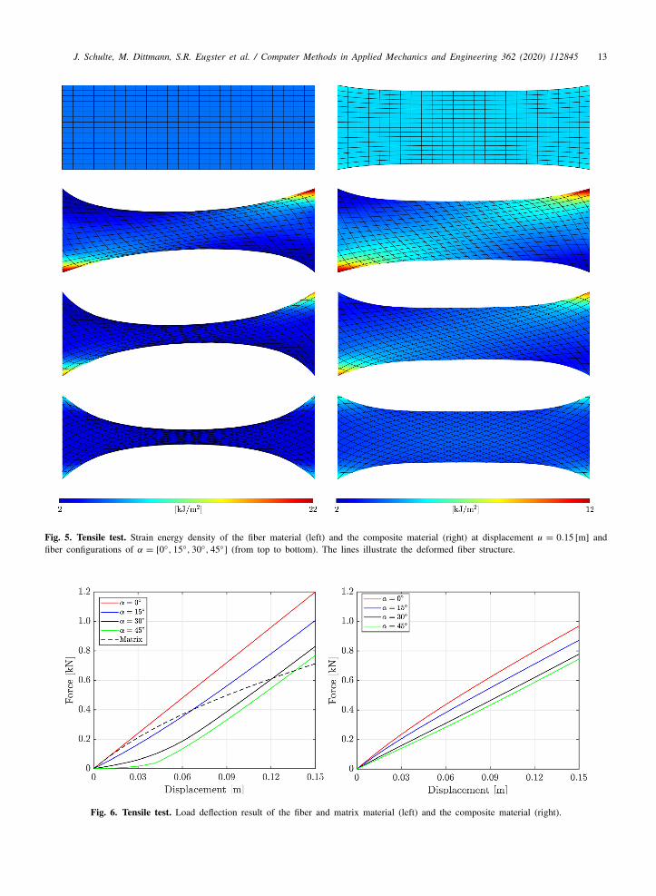
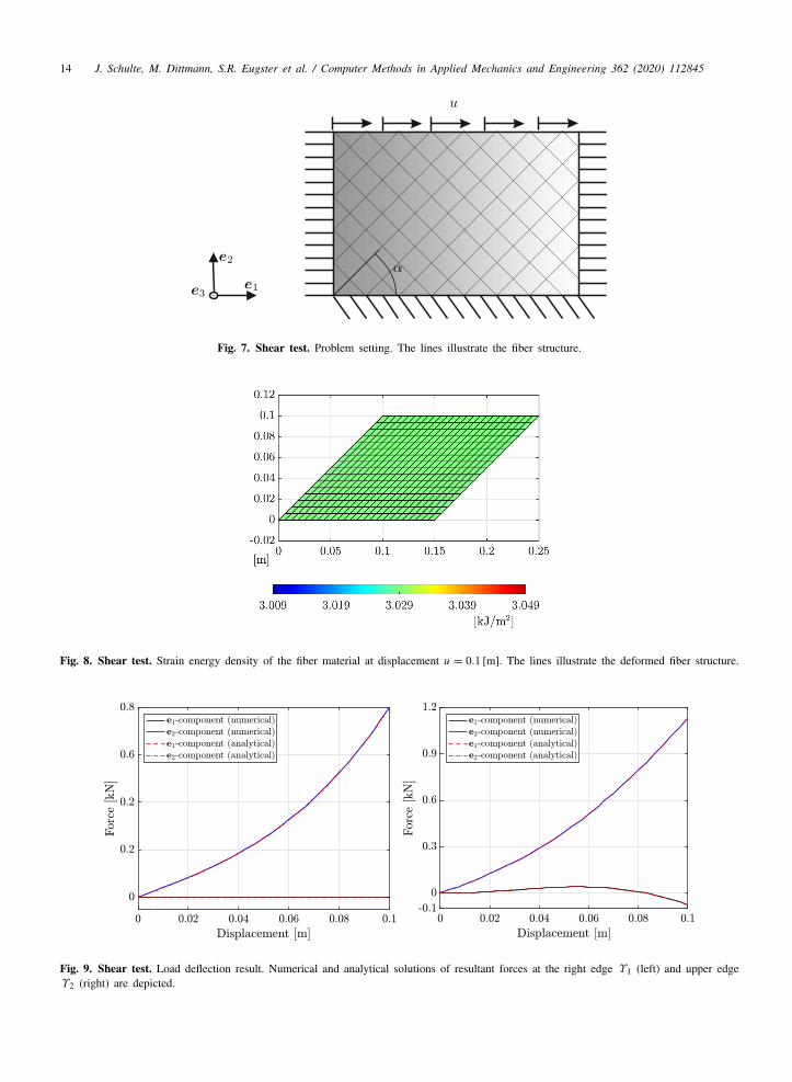
Figs. 8 and 9 show the distribution of the strain energy density and the load deflection result, respectively.Therein, we obtain a homogeneous strain energy density of 3029.3 [J/m2]. The obtained results are in accordanceto analytical solutions, see Appendix D for a detailed derivation.


Fig. 5. Tensile test. Strain energy density of the fiber material (left) and the composite material (right) at displacement u = 0.15 [m] andfiber configurations of α = [0, 15, 30, 45] (from top to bottom). The lines illustrate the deformed fiber structure.

Fig. 6. Tensile test. Load deflection result of the fiber and matrix material (left) and the composite material (right).


Fig. 7. Shear test. Problem setting. The lines illustrate the fiber structure.

Fig. 8. Shear test. Strain energy density of the fiber material at displacement u = 0.1 [m]. The lines illustrate the deformed fiber structure.

Fig. 9. Shear test. Load deflection result. Numerical and analytical solutions of resultant forces at the right edge Υ1 (left) and upper edgeΥ2 (right) are depicted.


Fig. 10. Out-of-plane bending test. Problem setting. The lines illustrate the fiber structure.

Fig. 11. Out-of-plane bending test. Configuration of the shell and strain energy distribution at different load steps. Pure matrix material(left) and pure fiber material (right) are applied. The lines illustrate the deformed fiber structure.

5.1.3. Out-of-plane bending testFor the out-of-plane bending test, the left edge of a shell is clamped and the right edge is subject to an external

out-of-plane torque µ = Me2 as shown in Fig. 10. In contrast to previous tests, the shell used for this test has alength of l = 1 [m] and a width of b = 0.1 [m] in the reference configuration, see Fig. 11. Using a thickness ofh = 0.002 [m] for pure matrix material and a thickness of hf = 0.002 [m] for pure fiber material, the area momentof inertia is obtained by I = bh3/12 = bh3

f /12 = 66.6667 [mm4]. The applied torque M = 2π E I/ l is chosen suchthat the shell describes a perfect circle in the asymptotic limit (see e.g. [36]) which holds for the fiber material bysetting α = 0, a1 = hf E = 12 [kN/m] and k1 = E I/b = 0.004 [Nm]. Moreover, for the matrix material we applythe compressible model given in (80) with µ = E/2 = 3 [MPa] and κ = E/3 = 2 [MPa] which corresponds toPoisson ratio of ν = 0.

In Fig. 11, the configuration of the shell is plotted along with the strain energy distribution for pure matrix andpure fiber material at different load steps. The results shown therein are obtained by 80 × 8 cubic B-spline basedelements. Moreover, Fig. 12 shows the convergence properties for both materials, where the error is determined asgap between the ends of the shell. Here, we observe a limit of convergence at a value of approximately 10−4 [m]for pure matrix material, whereas for pure fiber material an error of less than 2 · 10−8 [m] is obtained. Note thatthe limit of convergence using pure matrix material can be justified by known locking effects of Kirchhoff–Loveshell elements as it may occur even for high polynomial approximations, see e.g. [44–50]. In addition, the usageof an internal Newton–Raphson iteration within the implementation of a compressible Neo-Hookean model for thematrix material also limits the convergence.


Fig. 12. Out-of-plane bending test. Convergence results.

Fig. 13. In-plane bending test. Problem setting. The lines illustrate the fiber structure.

Next, a verification of the in-plane bending behavior of the fiber material is demonstrated. Therefore, we use theshell mesh defined for the out-of-plane bending test and set α = 0, a1 = hf E = 12 [kN/m] with hf = 0.002 [m]and g1 = g2 = E I/b = 10 [Nm] with I = hfb3/12 = 166 667 [mm4]. All other parameters of the fiber materialare set equal to zero. Moreover, we apply µ = Me3 as an external in-plane bending torque, see Fig. 13 for details.Again, the applied torque M = 2π E I/ l is chosen such that the shell describes a perfect circle in the asymptoticlimit, which is demonstrated in Fig. 14. Even if this result is not physically reasonable for a real composite due tothe material penetration, it verifies the implementation related to in-plane bending of pure fiber material.

5.1.4. In-plane bending test5.1.5. Torsion test

Eventually, we verify the numerical framework related to a torsional deformation of the fiber material, see Fig. 15.Therefore, the deformation is predetermined such that the shell undergoes a constant twist of ∂φ/∂ X1 = 1200 [/m]with X1 = X · e1. Moreover, the parameters of the fiber material are defined by hf = 0.002 [m] and k3 = µIp/b =

5.002 [Nm] with a polar moment of inertia Ip = bhf(b2+ h2

f )/12 = 166 733 [mm4]. Again, all other parameters areset equal to zero.

Strain energy densities obtained at ∆φ = 180 are depicted in Fig. 16 for different fiber configurations. Asexpected, we obtain a highly stressed region along the central axis of the shell especially in the 0 fiber configuration,whereas the fiber material does not contribute to the strain energy in the 45 configuration since the fibers are nottwisted. This is also evident in Fig. 17, where the twist of fiber is plotted for fiber configurations of α = 0 andα = 45. Concerning the 0 configuration, fibers in e1-direction undergo a twist of ∂φ/∂ X1 = 1200 [/m] atthe central axis of the shell. Moreover, analytical details related to the torsional test can be found in Appendix Everifying the numerical results shown in Fig. 16.

5.2. Calibration and validation

As introduced in Section 1.2, we investigate Tepex®dynalite 102-RG600(1)/47 from LANXESS as prototypicalcomposite material, consisting of 47% vol. of a woven fabric (roving glass) and polycaprolactam (PA 6) as matrix


Fig. 14. In-plane bending test. Configuration of the shell and strain energy distribution at different load steps using pure fiber material.The lines illustrate the deformed fiber structure.

Fig. 15. Torsion test. Problem setting. The lines illustrate the fiber structure.

material. The matrix material is hydrophilic with a maximum absorption of moisture between 2.6% and 3.4%. Forthe investigations presented here, a single layer material with layer thickness of 0.5 [mm] has been specificallymanufactured for this test, since multi-layered material with different fiber angles intermix various physical effectswithin the measurements.

The surrounding matrix material stiffens the woven fabric and connects the junctions of the fibers. The fiberswithin the composite material have significant bending stiffness due to the matrix material surrounding every singlestring within the fibers. Additional stiffening mechanisms are present depending on the actual weave of the wovenfabric, since the fibers are subject to frictional behavior at the junctions. These effects arise only for the combinedcomposite material and thus, cannot be separated within the experimental investigations, i.e. we always obtain amean value of the material characteristics.

Remark 3. The matrix material is in general governed by a far more complex constitutive behavior in the inelasticregime. Moreover, fibers and matrix might separate in the presence of large deformations, i.e. both materials canbe characterized by separately assigned deformation fields, coupled via corresponding constitutive laws. For now,we restrict ourself to the hyperelastic regime without fiber separation.


Fig. 16. Torsion test. Strain energy distribution of the fiber material at ∆φ = 180 using different fiber configurations α = [0, 15, 30, 45](from left to right and top to bottom). The lines illustrate the deformed fiber structure.

5.2.1. Experimental setupFor the tests on the fiber reinforced material, standard specimens with 125 [mm] × 25 [mm] and 125 [mm] ×

36 [mm] were prepared and pulled with 0.5 [mm/s] on a universal testing machine. To prevent slipping between thetesting machine and the specimen, considerable clamping forces are required. To preserve the underlying materialfrom fracturing due to the clamping forces, additional 20 [mm] cap strips (width is adjusted to the sample) madefrom the same material with fiber orientation rotated 45 against the orientation of the fibers of the samples wereglued at both sides at the ends of the specimen. Fig. 18 displays the clamping device for a 36 [mm] specimen.

For the digital image correlation measurements of the fiber reinforced material, the optical system Q400 fromLimess & Software GmbH was used. The evaluation of the images was done in Instra4D, version 4.1. For theanalysis, Instra4D generates a quadratic mesh within the region of interest with an element size of 5 pixels. At eachnode of the mesh, a facet of 29 pixels was applied, i.e. each facet is slightly larger compared to a single element ofthe correlation mesh. Note that at least one characteristic object of the speckle-pattern has to be inside every facet.


Fig. 17. Torsion test. Twist of fiber at ∆φ = 180 using a fiber configuration of α = 0 (left) and 45 (right). The lines illustrate thedeformed fiber structure.

Fig. 18. Clamping devise with 36 mm specimen, undeformed configuration.

To control the calculated strains, the position of each identified object in the current configuration was calculatedback into the reference configuration and compared with the original picture with a maximum tolerance of 0.3 pixel.

In Fig. 19, the measurements until failure of the 25 [mm] specimen with 30 fiber orientation are presented. Ascan be seen, a damage process starts after 0.4 [mm] corresponding to a load of 500 [N] and the fracture processbegins at a displacement of approximately 6 [mm]. In particular, the fibers start to rupture as indicated by thepost-fracture curves. Since we are interested in the elastic material behavior, we restrict the following diagrams tothe regions of interest.

5.2.2. ResultsTension test. We first elaborated tension tests with 0, 15, 30 and 45 fiber orientation. Here, experimental dataof 25 [mm] specimen are compared with numerical results using 34 × 10 cubic elements. Shear and bulk modulusused within the compressible model (80) for the PA 6 matrix material are assumed to be µ = 384.62 [N/mm2]and κ = 833.33 [N/mm2], respectively. This setting corresponds to Young’s modulus of Eiso = 1000 [N/mm2]and Poisson ratio of ν = 0.3. Moreover, for the glass fibers we assume Efib = 73 000 [N/mm2]. The thicknessof the material is h = 0.5 [mm], with 47% vol. of woven fabric, from which 50% are aligned in L and Mdirection, respectively. Thus, we obtain the material constants for the fiber stretch contributions via 0.5hEfib × 0.47as a1/2 = 8577.5 [N/mm], which corresponds to a combined Young’s modulus of 17 685 [N/mm2]. As can be seenin Fig. 20 for the 0 fiber orientation, the simulation fits perfectly the experiments.

The value for a3 = 250 [N/mm] is related to the interaction between the fibers and cannot be derived from otherconstants. Thus, we have fitted the value to the experimental observation obtained by a fiber orientation of 45,


Fig. 19. Experimental force–displacement curves for 25 mm specimen with 30 fiber orientation.

Fig. 20. Force–displacement curves of the tension test for 25 mm specimen with 0, 15, 30 and 45 fiber orientation (left to right, top todown). Simulation results are compared with experimental investigations. Additionally, simulation results without in-plane bending stiffness(Sim. wb) are shown to highlight the global effect of the non-classical in-plane curvature term.


Fig. 21. 4-point bending test, deformed configuration.

see Fig. 20 (right, bottom). The bending stiffness g1 = g2 on the other hand is related to Young’s modulus viag1/2 = Efib I/b = 893 500 [Nmm], where the second moment of inertia is I = b3hf/12 with hf = 0.47h. Note thatthis approach is only a motivation for choosing the material constants g1 and g2, since this allows us a comparisonwith analytical results as shown in Section 5.1.4. The values k1/2/3 do not contribute in these tension tests and g3 wasset to zero. Additional simulation results presented in Fig. 20 demonstrate the effects of the in-plane bending term,i.e. we set g1 = g2 = 0, to compare the results with an anisotropic Kirchhoff–Love shell formulation neglectingthe higher gradient terms.

This example shows that the bending stiffness has considerable effects on the global stiffness and is not negligible.The constitutive parameters chosen with respect to the different matrix and fiber materials and the respectivegeometry allow for a nearly perfect prediction of the macroscopic behavior of this material with microstructure.Only the parameter a3 is fitted, since the shear stiffness of the fibers depends on the weave of the fabric and theproduction process in terms of applied pressure, heat and cooling rate. This result illustrates the necessity to includehigher gradient terms in the model for fiber reinforced polymers.

Bending test. Next, we investigate the out-of-plane bending stiffness, hence we validate the values for k1 andk2. Therefore, a 4-point bending test as shown in Fig. 21 is conducted. For the experiments, a stack of 5specimen with 125 [mm] × 25 [mm] in 0 fiber configuration were used, such that we expect a stiffness of 5 timesk1/2 = Efib I/b = 78.949 [Nmm], where I = bh3

f /12 and hf = 0.47h. The support structure has a width of 40 [mm]between the inner brackets, and 30 [mm] between the outer and the inner brackets, such that the whole device hasa width of 100 [mm].

For the numerical validation, we discretize the shell with 50 × 10 cubic elements with prescribed displacementsin upward direction at the contact points of the support structure, such that the shell can slide over the bracket pointsand the system is subject to pure bending. The results in Fig. 22 demonstrate the consistency of the formulation withthe experimental observations until a displacement of about 15 [mm]. Afterwards, inelastic effects can be observed,resulting in a permanent deformation of the sample as can be observed in Fig. 23. After a displacement of 25 [mm],the sample starts to slip over the brackets.

Digital image correlation. Finally, we show in Fig. 24 (top) the results of the Digital image correlation for the25 [mm] specimen with 45 fiber orientation and a total displacement on the left boundary of 4.6 [mm]. Note


Fig. 22. Force–displacement curves of the out-of-plane bending test for a 25 [mm] specimen with 0 fiber orientation. Simulation resultsare compared with experimental investigations.

Fig. 23. 4-point bending test, permanent deformation of the sample after a full loading cycle.

that both sides are clamped in such a way that the displacement is prescribed and, additionally, the higher-orderboundary conditions are also set, preventing in-plane twist and torsion of the fibers. A direct comparison withsimulation results is not feasible, since the current model does not incorporate elastic softening or inelastic effectsof the polymeric matrix material. However, we want to highlight the strain gradient effects in terms of the resultingdeformation patterns. Therefore, the stiffness of the matrix material Eiso and the bending stiffness g1 and g2 isreduced by a factor of 500 to fit the globally reduced stiffness of the inelastic deformed composite.3 In both plotsin Fig. 24 the strain gradient effects result in the stiffness of the fibers against in-plane bending, which can beobserved at the crosspoint of the fibers as highlighted by the red line.

Using the same material setting, we compare next results for a 36 [mm] specimen in 30/60 configuration, seeFig. 25. As can be seen, the deformation patterns fit in general, although the fibers at the vertices of the samplealready start to fracture.

As final result of this section, we summarize the determined and validated material setting of our prototypicalcomposite material Tepex®dynalite 102-RG600(1)/47 in Table 2.

3 The bending stiffness of the pure fiber is nearly zero, but contribute considerably to the global stiffness if the fibers are embeddedwithin the matrix material. If the matrix is subject to inelastic effects, the bending stiffness is effected as well. Note that we have observedpronounced inelastic deformations by evaluating hysteresis curves. A detailed investigation of inelastic effects including plastification of thematrix material and fiber pullout is beyond scope of the current work, but will be part of a future contribution.


Fig. 24. DIC measurement of a 25 [mm] specimen in 45 configuration (top) and simulation results (bottom) at 4.6 [mm] total displacement,colors indicate local stretches in horizontal direction in [mm/m]. Black lines indicate the fiber direction in the current configuration. (Forinterpretation of the references to color in this figure legend, the reader is referred to the web version of this article.)

Fig. 25. DIC measurement of a 36 [mm] specimen in 60 configuration (top) and simulation results (bottom) at 4.6 [mm] total displacement,colors indicate local stretches in horizontal direction in [mm/m]. (For interpretation of the references to color in this figure legend, the readeris referred to the web version of this article.)

Remark 4. Warp and weft direction are given in 0 and 90 direction, respectively. Both exhibit a slightly differentmaterial behavior and are not perfectly aligned due to the production process. This can be calibrated using differentvalues for a1/2 and g1/2, which we omit here since the general behavior of this second gradient material is the keyissue in this paper.

5.3. Concluding example

This last example demonstrates the applicability of the proposed model to complex geometries with non-planarreference configurations. Therefore we consider a shaft of length 50 [mm] and radius 50/π [mm] as shown in Fig. 26,using the validated material setting given in Table 2. Additionally, we set g3 = 0 and k3 = 0. The discretization of theshaft consists of 200 cubic B-spline based elements. To obtain a closed cylinder, the extended Mortar method [40]is applied between the opposing edges in peripheral direction of the shell, maintaining G1-continuity, see alsoDittmann et al. [51,52] for more details. The displacement on the left in e2-direction of the cylinder is fixed in


Table 2Material setting of Tepex®dynalite 102-RG600(1)/47.

Compressible matrix material (PA 6)

Shear modulus µ 384.62 [N/mm2]Bulk modulus κ 833.33 [N/mm2]

Fiber material (roving glass)Tensile stiffness a1, a2 8577.5 [N/mm]Shear stiffness a3 250 [N/mm]In-plane bending stiffness g1, g2 893 500 [Nmm]Out-of-plane bending stiffness k1, k2 78.949 [Nmm]

Fig. 26. Concluding Example. Problem setting and computational mesh.

Fig. 27. Concluding Example. Strain energy density of the matrix material.

space, whereas the displacement on the right is fixed on the (e1, e3)-plane and rotated as illustrated in Fig. 26. Notethat no higher order boundary conditions according to (60)3 and (61) are applied.

First, we investigate a pure matrix material. After a prescribed angle of ∆φ = 3.3, the shell starts to buckle.The last state of equilibrium is obtained at an angle of ∆φ = 12.6, see Fig. 27. Note that e.g. an arc length methodcan be used to calculate further states in the geometrically unstable regime. In Fig. 28, the applied torque necessaryto obtain the prescribed twist at the right hand side of the shell versus the angle of twist ∆φ is plotted for the purematrix as well as for the composite material with different fiber orientations with and without the in-plane bendingterms.


Fig. 28. Concluding Example. Torque versus angle of twist. Displayed are the results for the pure matrix material, the composite and thecomposite without the additional in-plane contributions (composite*).

Next, the composite material is investigated. In Fig. 29, upper left, the strain energy for a 0 fiber configurationafter a prescribed twist of ∆φ = 90 is displayed. Note that the fiber orientation and not the computational mesh isshown. The corresponding torque is given again in Fig. 28. Several issues can be highlighted here. First, the higherorder boundary conditions as presented in (60)3 are not set and thus, the fibers can twist in-plane at the boundary.This can be observed very well in Fig. 29, upper left. If bending would be prohibited at the boundary, the fibershave to remain orthogonal with regard to the boundary. Since these additional boundary conditions are unknownto a first gradient theory or even to the classical Kirchhoff–Love shell theory which only considers the out- andnot the in-plane contributions, the proposed formulation is the only way to enforce this consistently within themechanical formulation. Second, the in-plane terms stabilize the shell against buckling. Fig. 30, upper left, showsthe results if the additional in-plane terms are not present, i.e. the material constants g1 and g2 are set to zero. Thus,we obtain the results for an anisotropic Kirchhoff–Love formulation, usual fitted via a first-gradient homogenizationprocess, showing large buckling modes. To illustrate this further, the strain energy of the in-plane contributions forthe deformed configuration (cf. Fig. 30, upper left) is plotted in Fig. 31. As can be observed, a dramatic increaseof the in-plane strain energy occurs for this heavily deformed configuration, hence, in the mechanical equilibriumthis buckling mode is not possible.

Additionally, results for 15, 30 and 45 fiber orientation are plotted (upper right, lower left and lower rightpicture in Figs. 29 and 30). The corresponding torque is plotted again in Fig. 28. Notably, a nearly constant strainenergy distribution can be observed in Fig. 29, lower right and upper left.

6. Conclusions

In this paper, we formulate a Kirchhoff–Love shell theory to account for in-plane bending flexure resistanceof embedded fibers. More specifically, the proposed formulation addresses in total additional twelve curvaturecomponents. Based on this set of deformation measures, we can now apply standard 3D constitutive laws to theshell continuum and combine them with the contribution of the woven fabric to describe composite materials inthe hyperelastic regime. Moreover, the localization allows us to identify the corresponding boundary terms, whichaccount for additional Dirichlet and Neumann contributions as required by fourth-order partial differential equation.

The verification and adjustment of the corresponding material parameters allows us to identify the physical effectsof the higher-order terms in this prototypical second gradient material. Based on this verification step, we can nowfor the first time calibrate and validate a second gradient formulation using experimental results for fiber reinforced


Fig. 29. Concluding Example. Strain energy density of the composite material with different fiber orientations α = [0, 15, 30, 45] (fromleft to right and top to bottom) plotted at the final deformation state marked in Fig. 28.

material. This material is composed of a first gradient polymeric material and a second gradient woven fabric madeof glass fiber.

Thus, we are now able to conduct simulations in the hyperelastic regime of this complex material behavior.Further developments will incorporate additional inelastic properties along with fracture mechanisms, as proposede.g. in Dittmann et al. [53,54] and Aldakheel et al. [55].

Acknowledgments

Support for this research was provided by the Deutsche Forschungsgemeinschaft (DFG), Germany undergrant HE5943/8-1. This support is gratefully acknowledged. The authors M. Dittmann and C. Hesch gratefullyacknowledge support by the DFG, Germany under grant DI2306/1-1. The authors gratefully acknowledge the helpof Heiko Bendler at the Institute of Mechanics (IFM) at the Karlsruhe Institute of Technology (KIT) to performthe experimental investigations on organic sheets. Finally, we thank an anonymous referee for detailed and helpfulcomments within the review process.

Appendix A. Frame invariance

To demonstrate the invariance of the introduced measures aαβ, κα,β, Sσα,β under superposed rigid body motions

we define rigid motions of the form

r+:= u + Qr , (81)

where u ∈ E3 and Q ∈ SO(3) is a rotation tensor with the property QT Q = I . Then, the first and second partialderivative read

a+

α = Qr ,α and a+

αβ = Qr ,αβ . (82)


Fig. 30. Concluding Example. Strain energy density of the composite material with different fiber orientations α = [0, 15, 30, 45] (fromleft to right and top to bottom) without in-plane contributions plotted at the final deformation state marked in Fig. 28.

Fig. 31. Concluding Example. Estimated strain energy density of the in-plane contribution using the deformed configuration in 30, upperleft.

Starting with the covariant metric coefficients one gets

a+

αβ = a+

α · a+

β = ( Qr ,α) · ( Qr ,β) = r ,α · QT Q =I

r ,β = aαβ (83)


which clearly holds also for the contravariant metric coefficients, i.e. (aαβ)+ = aαβ . With respect to this result, wecan show

S+

αβλ = Γ+

αβλ − Γ λαβa+

αλ = ( Qr ,λ) · ( Qr ,αβ) − Γ λαβaαλ = r ,λ · QT Q

=I

r ,αβ − Γ λαβaαλ = Sαβλ (84)

as well as

(Sσαβ)+ = S+

αβλ(aσλ)+ = Sαβλaσλ= Sσ

αβ , (85)

i.e. the frame invariance of the co- and contravariant in-plane curvature tensor is confirmed. Eventually, we obtainfor the out-of-plane curvature tensor

κ+

αβ = Bαβ − b+

αβ

= Bαβ − Qr ,αβ ·Qa1 × Qa2

∥ Qa1 × Qa2∥

= Bαβ −det( Qr ,αβ, Qa1, Qa2)√

det(a+

αβ)

= Bαβ − det( Q) =1

det(r ,αβ, a1, a2)√det(aαβ)

= καβ .

(86)

confirming again the frame invariance. Note that frame invariance of the deformation measures imply translationalas well as rotational invariance of the strain energy which in turn implies satisfaction for conservation of linear andangular momentum, see Hesch & Betsch [56] and Marsden & Ratiu [57] for further details.

Appendix B. Fiber deformation measures

To obtain more insight into the fiber deformation measures (24)–(27), we derive them in the following fromthe conception that the fibers are modeled as mathematical curves with appropriate kinematical and constitutivestructure to capture the mechanical properties of the reinforcement. Besides the applied formulation as functionsof aαβ , Sσ

αβ , καβ and θα , we show alternative representations in terms of stretch and curvature quantities given tomathematical curves.

The unit tangents to the fibers on ω are denoted by l and m. Since these vectors are necessarily tangent to themid-surface, they can be represented as

l = lαaα and m = mαaα. (87)

For the description of the fibers in the reference mid-surface Ω , we introduce the tangents L and M, which do notnecessarily have unit length but which are orthogonal to each other and can be written as

L = Lα Aα and M = Mα Aα. (88)

Since the fibers are convected as material curves, the tangent vectors are related by

λ1l = FL

∥L∥and λ2l = F

M∥M∥

(89)

where we made use of the fiber stretches

λ1 :=

FL∥L∥

=

√aαβ Lα Lβ√Aµν LµLν

and λ2 :=

F M∥M∥

=

√aαβ Mα Mβ√Aµν MµMν

. (90)

Therefore, the corresponding contravariant components are connected by

Lα= λ1∥L∥lα =

√aµν LµLνlα and Mα

= λ1∥M∥Mα=√

aµν MµMνmα. (91)

The change of angle between the fibers can be easily obtained as

ϕ := acos

(Aαβ Lα Mβ√


)− acos

(aαβ Lα Mβ√


). (92)


For initially orthonormal fibers, the first term is certainly π/2.To study the change of the tangent vectors l and m within the deformed mid-surface, we introduce the auxiliary

unit tangent vectors

p = n × l , q = n × m. (93)

Moreover, let l : B → E3 and m : B → E3 be such that

l(θα) = l(r(θα)) and m(θα) = m(r(θα)) . (94)

Then the gradients

∇ l(r) = l ,α ⊗ aα and ∇m(r) = m,α ⊗ aα (95)

are easily obtained by inserting dθα= dr · aα into the expressions dl = l ,α dθα

= l ,α( dr · aα) = (l ,α ⊗ aα) drand dm = m,α dθα

= (m,α ⊗ aα) dr , respectively. Since ∥l∥ = ∥m∥ = 1, we have l · l ,α = m · m,α = 0 and thepartial derivatives of the unit vectors l and m can be expressed in the right-handed orthonormal bases l, p, n andm, q, n as

l ,α = (l ,α · p) p + (l ,α · n)n and m,α = (m,α · q)q + (m,α · n)n. (96)

Using (87) together with the Gauss and Weingarten equation (6), the normal components in (96) can be expressedusing the covariant components of the mid-surface curvature bαβ as

l ,α · n = (lβ aβ),α · n = lβbβα and m,α · n = (mβ aβ),α · n = mβbβα. (97)

The change of the unit tangent vectors in tangential direction can therefore be represented by

∇ l(r)l = lα l ,α = ηl p + κl n and ∇m(r)m = mαm,α = ηm q + κm n (98)

with the normal fiber curvatures

κl := bαβlαlβ =bαβ Lα Lβ

aµν LµLνand κm := bαβmαmβ

=bαβ Mα Mβ

aµν MµMν(99)

and the geodesic curvatures

ηl := lα l ,α · p and ηm := mαm,α · q. (100)

The change of the unit tangent vectors of one fiber family in direction of the other fiber family leads to

∇ l(r)m = mα l ,α = φl p + τn and ∇m(r)m = mαm,α = φm q + τn , (101)

where we recognize the torsion and the respective Tchebychev curvatures, [18],

τ := bαβlαmβ=

bαβ Lα Mβ√aµν LµLνaσρ Mσ Mρ

, φl := mα(l ,α · p) , φm := lα(m,α · q). (102)

Similarly to (99) and (102), we can introduce the normal fiber curvatures κL , κM and the torsion τ on the referencemid-surface as

κL :=Bαβ Lα Lβ

Aµν LµLν, κM :=

Bαβ Mα Mβ

Aµν MµMνand τ :=

Bαβ Lα Mβ√Aµν LµLν Aσρ Mσ Mρ

. (103)

Because these definitions rely on unit tangent vectors, the normalization by ∥L∥ and ∥M∥ are involved in here.As deformation measures that captures the change in the normal curvature of the fibers, i.e. by out-of-plane

bending, we choose

K1 := −καβ Lα Lβ

Aµν LµLν= λ2

1κl − κL and K2 := −καβ Mα Mβ

Aµν MµMν= λ2

1κm − κM . (104)

The change in torsion by twisting the fibers is given by

K3 := −καβ Lα Mβ√

Aµν LµLν Aσρ Mσ Mρ= λ1λ2τ − τ . (105)


Finally, to describe the deformation of the fibers within the tangent planes of the mid-surfaces, like in-plane-bending,we introduce as strain measures

gL :=Lα Lβ Sαβσ

Aµν LµLνaσ , gM :=

Mα Mβ Sαβσ

Aµν MµMνaσ and Γ :=

Lα Mβ Sαβσ√Aµν LµLν Aσρ Mσ Mρ

aσ . (106)

For initially straight fibers, the deformation measures (106) can be represented as

gL = λ1ηl p + (L · ∇λ1)l , gM = λ2ηm q + (M · ∇λ2)mΓ = (L · ∇λ2)m + λ1λ2φm q = (M · ∇λ1)l + λ1λ2φl p ,

(107)

with the stretch gradients as ∇λ1 = λ1,α Aα and ∇λ2 = λ2,α Aα (see Equation (58) and (59) in [20]). We referto Section 2.4 of [20], where also the general precurved situation is analyzed. However, the restriction to straightfibers lies only in the representation (107), which should help to get more insight into strain measures (106). Infact, these strain measures obtained by the contraction of the fiber tangents of the reference mid-surface with thethird order tensor aσ ⊗ Sσ represent a combination of the gradients of the fiber stretch and in-plane-deformationof the fibers described by geodesic and Tchebychev curvatures.

Appendix C. Stress resultants

Applying the strain energy function of the matrix material given in (41) and using [Cαβ] = [Cαβ]−1 togetherwith

∂

∂Cµν

( 1

det(Cαβ)

)= −

1

det(Cαβ)2det(Cλσ )Cµν

= −Cµν

det(Cαβ)(108)

we get

∂Ψ iso

∂Cµν

=12µ

(Gµν

−det(Gµν)

det(Cαβ)Cµν

)(109)

that has to be integrated in thickness direction to obtain the stress resultants.The corresponding stress resultants of the first term (36)1 reads

nαβ

fib =∂Ψfib

∂λ1

∂λ1

∂aαβ

+∂Ψfib

∂λ2

∂λ2

∂aαβ

+∂Ψfib

∂ϕ

∂ϕ

∂aαβ

+∂Ψfib

∂Cσµ

∂Cσµ

∂aαβ

=a1(λ1 − 1)∂λ1

∂aαβ

+ a2(λ2 − 1)∂λ2

∂aαβ

+ 2a3tan(ϕ)

cos2(ϕ)∂ϕ

∂aαβ

+

(g1

(Lγ LλSγ λσ )(Lζ L ιSζ ιµ)(Aµν LµLν)2 + g2

(Mγ MλSγ λσ )(Mζ M ιSζ ιµ)(Aµν MµMν)2

+ g3(Lγ MλSγ λσ )(Lζ M ιSζ ιµ)


)∂Cσµ

∂aαβ

,

(110)

where we have made use of (42) as strain energy function of the fiber material and

gL · gL =(Lα Lβ Sαβσ )(Lγ LλSγ λµ)Cσµ

(Aµν LµLν)2 ,

gM · gM =(Mα Mβ Sαβσ )(Mγ MλSγ λµ)Cσµ

(Aµν MµMν)2 ,

Γ · Γ =(Lα Mβ Sαβσ )(Lγ MλSγ λµ)Cσµ

Aµν LµLν Aσρ Mσ Mρ.

(111)

Moreover, the relations

∂λ1

∂aαβ

=12

Lα Lβ√aσλLσ Lλ Aµν LµLν

,∂λ2

∂aαβ

=12

Mα Mβ√aσλMσ Mλ Aµν MµMν

(112)


and

∂ϕ

aαβ

=1√

1 −(aαβ Lα Mβ )2


(Lα Mβ√


−aαβ Lα Mβ

2(aµν LµLνaσρ Mσ Mρ)3/2 (aµν LµLν Mσ Mρ+ LµLνaσρ Mσ Mρ)

) (113)

as well as the partial derivative of the contravariant metric

∂Cσµ

∂aαβ

=∂Cσµ

∂Cαβ

= −CσαCβµ (114)

have been used. For the second term (36)2, the stress resultants of the out-of-plane bending moments reads

mαβ

fib = −k1 K1Lα Lβ

Aµν LµLν− k2 K2

Mα Mβ

Aµν MµMν− k3 K3

Lα Mβ√Aµν LµLν Aσρ Mσ Mρ

, (115)

whereas the third term (36)3 yields

mαβσ

fib =g1Lα Lβ(Lγ LλSγ λµ)

(Aµν LµLν)2 Cσµ+ g2

Mα Mβ(Mγ MλSγ λµ)(Aµν MµMν)2 Cσµ

+

g3Lα Mβ(Lγ MλSγ λµ)

Aµν LµLν Aσρ Mσ MρCσµ .

(116)

Appendix D. Analytics – shear test

Assuming a linear parametrization of the reference mid-surface

r = θ1e1 + θ2e2 with θ1∈ [0, l] and θ2

∈ [0, b] , (117)

the analytical solution for pure fiber material with a fiber configuration of α = 0 can be derived as follows. Notethat we obtain A1 = e1 and A2 = e2 due to (117). The isochoric deformed configuration of the mid-surface shownin Fig. 8 is described by

r(θ1, θ2) =

(θ1

+θ2ub

)e1 + θ2e2 , (118)

where u is the predefined displacement of the upper boundary, see Fig. 7. Now, applying (4), (5), (24) and (25) weobtain

λ1 = 1, λ2 =

√(ub

)2+ 1 and ϕ =

π

2− acos

⎛⎝ ub√( u

b

)2+ 1

⎞⎠ (119)

as fiber stretches and the change of angle between the fibers, respectively. Insertion of the strain measures into (42)and (60) yields

Ψfib=

a2

2

(√(ub

)2+ 1 − 1

)2

+a3

2tan

⎛⎝π

2− acos

⎛⎝ ub√( u

b

)2+ 1

⎞⎠⎞⎠2

(120)

and after some straightforward calculations

N1= a3Π

⎡⎣010

⎤⎦ and N2= a2

⎛⎝1 −1√( u

b

)2+ 1

⎞⎠⎡⎣ ub10

⎤⎦+ a3Π( u

b

)2+ 1

⎡⎣ 1−

ub

0

⎤⎦ , (121)


where the abbreviation

Π =

tan

(π2 − acos

(ub√

( ub )

2+1

))

cos

(π2 − acos

(ub√

( ub )

2+1

))2 . (122)

is applied. Eventually, using (60) we can evaluate the resultant forces at the right boundary Υ1 and upper boundaryΥ2 as

FΥ1 =

∫Υ1

[N1 N2] νΥ1 dS = N1b and FΥ2 =

∫Υ2

[N1 N2] νΥ2 dS = N2l , (123)

respectively, where νΥ1 = [1, 0]T and νΥ2 = [0, 1]T are corresponding unit normal vectors. Thus, for the finaldeformation state, i.e. u/b = 1, we obtain

Ψfib(u = 0.1 [m]) ≈ 3029.3J

m2 (124)

as homogeneous strain energy distribution and the forces at the boundaries are

FΥ1 (u = 0.1 [m]) =

⎡⎣ 0800

0

⎤⎦ [N] and FΥ2 (u = 0.1 [m]) ≈

⎡⎣−72.81127.2

0

⎤⎦ [N] . (125)

Appendix E. Analytics – torsion test

Assuming a linear parametrization of the reference mid-surface, cf. (117), with θ1∈ [0, l] and θ2

∈ [−b/2, b/2]such that A1 = e1 and A2 = e2, strain energy distributions for pure fiber material with different fiber configurationscan be evaluated as follows. The predefined deformation of the mid-surface shown in Figs. 16 and 17, respectively,is described by

r(θ1, θ2) = θ1e1 + θ2 cos(

πθ1

l

)e2 + θ2 sin

(πθ1

l

)e3 . (126)

Applying (4), (7)2 and (23)2 we obtain

κ11 = κ22 = 0 and κ12 = κ21 = −π√

(θ2π )2 + l2. (127)

Concerning different fiber configurations defined by α, the vector fields L and M in the reference configuration aregiven by

L1= cos(α), L2

= sin(α), M1= − sin(α), M2

= cos(α) . (128)

Eventually, insertion of these derivations into (26)3 and (42) yields

Ψfib=

k3

2(K3)2

=k3

2π2

(θ2π )2 + l2 (cos(α)2− sin(α)2)2 . (129)

Note that for the evaluation all material parameters are set equal to zero excepted k3. Obviously, for the α = 45

fiber configuration, the strain energy distribution related to a torsional deformation of the shell is identical to zero,whereas for each other configuration, the highest value is obtained at the central axis of the shell, i.e. at θ2

= 0.We obtain for the α = 0 fiber configuration

Ψfib(θ2= 0) ≈ 1097.06

Jm2 and Ψfib(θ2

= b/2) = Ψfib(θ2= −b/2) ≈ 523.25

Jm2 , (130)

for the α = 15 fiber configuration

Ψfib(θ2= 0) ≈ 822.8

Jm2 and Ψfib(θ2

= b/2) = Ψfib(θ2= −b/2) ≈ 392.44

Jm2 (131)


and for the α = 30 fiber configuration

Ψfib(θ2= 0) ≈ 274.27

Jm2 and Ψfib(θ2

= b/2) = Ψfib(θ2= −b/2) ≈ 130.81

Jm2 . (132)

References[1] R.A. Mindlin, Second gadient of strain and surface-tension in linear elasticity, Int. J. Solids Struct. 1 (1965) 417–438.[2] P. Germain, The method of virtual power in continuum mechanics. Part 2: Microstructure, SIAM J. Appl. Math. 25 (1973) 556–575.[3] R. Toupin, Elastic materials with couple-stresses, Arch. Ration. Mech. Anal. 11 (1962) 385–414.[4] R.A. Toupin, Theories of elasticity with couple stress, Arch. Ration. Mech. Anal. 17 (1964) 85–112.[5] A.C. Eringen, E.S. Suhubi, Nonlinear theory of simple microelastic solids, Internat. J. Engrg. Sci. 2 (1964) 189–203, 389–404.[6] A.C. Eringen, D.G.B. Edelen, On nonlocal elasticity, Internat. J. Engrg. Sci. 10 (1972) 233–248.[7] A.C. Eringen, Microcontinuum Field Theories I: Foundations and Solids, Springer, 1999.[8] A. Eringen, G. Maugin, Electrodynamics of Continua I: Foundations and Solid Media, Springer, Dordrecht, Heidelberg, London, New

York, 1990.[9] G. Maugin, A. Metrikine, Mechanics of Generalized Continua. One Hundred Years After the Cosserats, Springer-Verlag New York,

2010.[10] S. Forest, R. Sievert, Elastoviscoplastic constitutive frameworks for generalized continua, Acta Mech. 160 (2003) 71–111.[11] C. Hirschberger, E. Kuhl, P. Steinmann, On deformational and configurational mechanics of micromorphic hyperelasticity - Theory

and computation, Comput. Methods Appl. Mech. Engrg. 196 (2007) 4027–4044.[12] K. Saanouni, M. Hamed, Micromorphic approach for finite gradient-elastoplasticity fully coupled with ductile damage: Formulation

and computational aspects, Int. J. Solids Struct. 50 (2013) 2289–2309.[13] N. Kirchner, P. Steinmann, A unifying treatise on variational principles for gradient and micromorphic continua, Phil. Mag. 85 (2005)

3875–3895.[14] A. Javili, F. dell’Isola, P. Steinmann, Geometrically nonlinear higher-gradient elasticity with energetic boundaries, J. Mech. Phys. Solids

61 (12) (2013) 2381–2401.[15] P. Neff, The cosserat couple modulus for continuous solids is zero viz the linearized Cauchy-stress tensor is symmetric, ZAMM 86

(2006) 892–912.[16] P. Neff, J. Jeong, A new paradigm: the linear isotropic cosserat model with conformally invariant curvature energy,, ZAMM 44 (2009)

574–594.[17] F. Yang, A. Chong, D. Lam, P. Tong, Couple stress based strain gradient theory for elasticity, Int. J. Solids Struct. 39 (2002) 2731–2743.[18] D. Steigmann, A. Pipkin, Equilibrium of elastic nets, Philos. Trans. R. Soc. Lond. 335 (1991) 419–454.[19] D. Steigmann, Theory of elastic solids reinforced with fibers resistant to extension, flexure and twist, Int. J. Non-Linear Mech. 47

(2012) 734–742.[20] D. Steigmann, F. dell’Isola, Mechanical response of fabric sheets to three-dimensional bending, twisting, and stretching, Acta Mech.

Sinica (2015).[21] D. Steigmann, Equilibrium of elastic lattice shells, J. Eng. Math. 109 (2018) 47–61.[22] F. dell’Isola, I. Giorgio, M. Pawlikowski, N.L. Rizzi, Large deformations of planar extensible beams and pantographic lattices: heuristic

homogenization, experimental and numerical examples of equilibrium, Proc. R. Soc. A 472 (2185) (2016).[23] F. dell’Isola, P. Seppecher, M. Spagnuolo, E. Barchiesi, F. Hild, T. Lekszycki, I. Giorgio, L. Placidi, U. Andreaus, M. Cuomo, S.

Eugster, A. Pfaff, K. Hoschke, R. Langkemper, E. Turco, R. Sarikaya, A. Misra, M. De Angelo, F. D’Annibale, A. Bouterf, X. Pinelli,A. Misra, B. Desmorat, M. Pawlikowski, C. Dupuy, D. Scerrato, P. Peyre, M. Laudato, L. Manzari, P. Göransson, C. Hesch, S.Hesch, P. Franciosi, J. Dirrenberger, F. Maurin, Z. Vangelatos, C. Grigoropoulos, V. Melissinaki, M. Farsari, W. Muller, B. Abali, C.Liebold, G. Ganzosch, P. Harrison, R. Drobnicki, L. Igumnov, F. Alzahrani, T. Hayat, Advances in pantographic structures: design,manufacturing, models, experiments and image analyses, Contin. Mech. Thermodyn. 31 (2019) 1231–1282.

[24] J. Fish, Practical Multiscaling, John Wiley & Sons, 2013.[25] H. Wang, H. Zhou, J. Mishnaevsky, P. Brondsted, L. Wang, Single fibre and multifibre unit cell analysis of strength and cracking of

unidirectional composites, Comput. Mater. Sci. 46 (2009) 810–820.[26] L. Mishnaevsky, Computational Mesomechanics of Composites: numerical Analysis of the Effect of Microstructures of Composites of

Strength and Damage Resistance, Wiley-Interscience, 2007.[27] C.B. Hirschberger, A Treatise on Micromorphic Continua. Theory, Homogenization, Computation (Ph.D. thesis), Lehrstuhl für

Technische Mechanik, Technische Universität Kaiserslautern, 2008.[28] G. Hütter, Homogenization of a Cauchy continuum towards a micromorphic continuum, J. Mech. Phys. Solids 99 (2017) 394–408.[29] T. Asmanoglo, A. Menzel, A finite deformation continuum modelling framework for curvature effects in fibre-reinforced nanocomposites,

J. Mech. Phys. Solids 107 (2017) 411–432.[30] T. Asmanoglo, A. Menzel, A multi-field finite element approach for the modelling of fibre-reinforced composites with fibre-bending

stiffness, Comput. Methods Appl. Mech. Engrg. 317 (2017) 1037–1067.[31] A. Spencer, K. Soldatos, Finite deformations of fibre-reinforced elastic solids with fibre bending stiffness, Int. J. Non-Linear Mech.

42 (2007) 355–368.[32] K. Soldatos, Second-gradient plane deformations of ideal fibre-reinforced materials: implications of hyper-elasticity theory, J. Eng.

Math. 68 (2010) 99–127.

http://refhub.elsevier.com/S0045-7825(20)30026-8/sb1












































































[33] T. Hughes, J. Cottrell, Y. Bazilevs, Isogeometric analysis: CAD, finite elements, NURBS, exact geometry and mesh refinement, Comput.Methods Appl. Mech. Engrg. 194 (39–41) (2005) 4135–4195.

[34] J. Cottrell, T. Hughes, Y. Bazilevs, Isogeometric Analysis: Toward Integration of CAD and FEA, Wiley, 2009.[35] P. Fischer, M. Klassen, J. Mergheim, P. Steinmann, R. Müller, Isogeometric analysis of 2D gradient elasticity, Comput. Mech. 47 (3)

(2011) 325–334.[36] J. Kiendl, K. Bletzinger, J. Linhard, R. Wüchner, Isogeometric shell analysis with Kirchhoff–Love elements, Comput. Methods Appl.

Mech. Engrg. 198 (2009) 3902–3914.[37] J. Kiendl, M. Hsu, M. Whu, A. Reali, Isogeometric Kirchhoff-Love shell formulations for general hyperelastic materials, Comput.

Methods Appl. Mech. Engrg. 291 (2015) 280–303.[38] V. Balobanov, J. Kiendl, S. Khakalo, J. Niiranen, Kirchhoff-Love shells within strain gradient elasticity: Weak and strong formulations

and an H3-conforming isogeometric implementation, Comput. Methods Appl. Mech. Engrg. 344 (2019) 837–857.[39] P. Ciarlet, An Introduction to Differential Geometry with Aplications to Elasticity, Springer, 2005.[40] S. Schuß, M. Dittmann, S. Klinkel, B. Wohlmuth, C. Hesch, Multi-patch isogeometric analysis for Kirchhoff-Love shell elements,

Comput. Methods Appl. Mech. Engrg. 349 (2019) 91–116.[41] P. Bornemann, F. Cirak, A subdivision-based implementation of the hierarchical b-spline finite element method, Comput. Methods

Appl. Mech. Engrg. 253 (2013) 584–598.[42] C. Hesch, S. Schuß, M. Dittmann, M. Franke, K. Weinberg, Isogeometric analysis and hierarchical refinement for higher-order phase-field

models, Comput. Methods Appl. Mech. Engrg. 303 (2016) 185–207.[43] M. Dittmann, Isogeometric analysis and hierarchical refinement for multi-field contact problems (Ph.D. thesis), University of Siegen,

2017.[44] M. Ishaquddina, P. Raveendranath, J. Reddy, Flexure and torsion locking phenomena in out-of-plane deformation of Timoshenko curved

beam element, Finite Elem. Anal. Des. 51 (2012) 22–30.[45] F. Auricchio, L. Beirão da Veiga, J. Kiendl, C. Lovadina, A. Reali, Locking-free isogeometric collocation methods for spatial Timoshenko

rods, Comput. Methods Appl. Mech. Engrg. 263 (2013) 113–126.[46] L. Greco, M. Cuomo, An isogeometric implicit G1 mixed finite element for Kirchhoff space rods, Comput. Methods Appl. Mech.

Engrg. 298 (2016) 325–349.[47] R. Echter, M. Bischoff, Numerical efficiency, locking and unlocking of NURBS finite elements, Comput. Methods Appl. Mech. Engrg.

199 (5–8) (2010) 374–382.[48] K. Bletzinger, M. Bischoff, E. Ramm, A unified approach for shear-locking-free triangular and rectangular shell finite elements, Comput.

Struct. 75 (3) (2000) 321–334.[49] R. Bouclier, T. Elguedj, A. Combescure, Efficient isogeometric NURBS-based solid-shell elements: Mixed formulation and B-method,

Comput. Methods Appl. Mech. Engrg. 267 (2013) 86–110.[50] L. Greco, M. Cuomo, L. Contrafatto, A reconstructed local B formulation for isogeometric Kirchhoff-Love shells, Comput. Methods

Appl. Mech. Engrg. 332 (2018) 462–487.[51] M. Dittmann, S. Schuß, B. Wohlmuth, C. Hesch, Weak Cn coupling for multi-patch isogeometric analysis in solid mechanics, Internat.

J. Numer. Methods Engrg. 118 (2019) 678–699.[52] M. Dittmann, S. Schuß, B. Wohlmuth, C. Hesch, Crosspoint modification for multi-patch isogeometric analysis, Comput. Methods

Appl. Mech. Engrg. 360 (2020) 112768.[53] M. Dittmann, F. Aldakheel, J. Schulte, P. Wriggers, C. Hesch, Variational phase-field formulation of non-linear ductile fracture, Comput.

Methods Appl. Mech. Engrg. 342 (2018) 71–94.[54] M. Dittmann, F. Aldakheel, J. Schulte, F. Schmidt, M. Krüger, P. Wriggers, C. Hesch, Phase-field modeling of porous-ductile fracture

in non-linear thermo-elasto-plastic solids, Comput. Methods Appl. Mech. Engrg. 361 (2020) 112730.[55] F. Aldakheel, P. Wriggers, C. Miehe, A modified Gurson-type plasticity model at finite strains: Formulation, numerical analysis and

phase-field coupling, Comput. Mech. 62 (4) (2017) 815–833.[56] C. Hesch, P. Betsch, Transient 3D domain decomposition problems: Frame-indifferent mortar constraints and conserving integration,

Internat. J. Numer. Methods Engrg. 82 (2010) 329–358.[57] J. Marsden, T. Ratiu, Introduction to Mechanics and Symmetry, Springer, 2003.






































































Isogeometric analysis of fiber reinforced composites using ...

Documents

Transcript of Isogeometric analysis of fiber reinforced composites using ...