ISENTROPIC POTENTIAL VORTICITY

•  Read Section 1.9 in Bluestein Vol. II

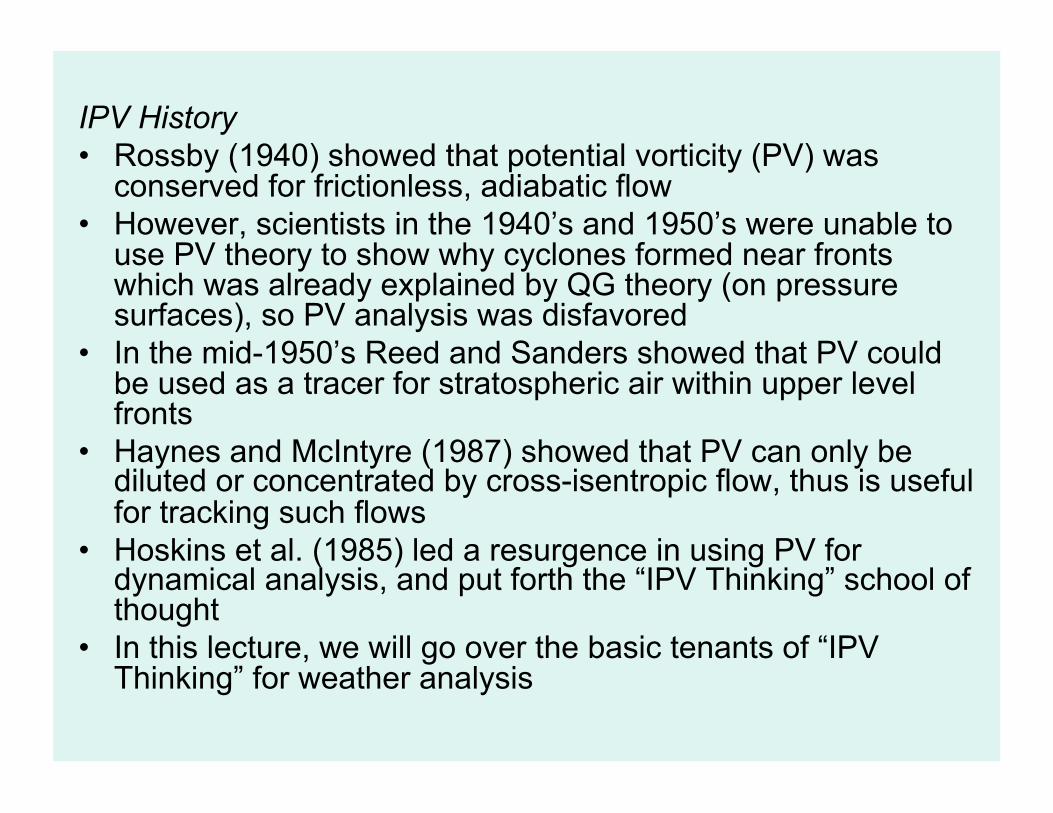
IPV History •  Rossby (1940) showed that potential vorticity (PV) was

conserved for frictionless, adiabatic flow •  However, scientists in the 1940’s and 1950’s were unable to

use PV theory to show why cyclones formed near fronts which was already explained by QG theory (on pressure surfaces), so PV analysis was disfavored

•  In the mid-1950’s Reed and Sanders showed that PV could be used as a tracer for stratospheric air within upper level fronts

•  Haynes and McIntyre (1987) showed that PV can only be diluted or concentrated by cross-isentropic flow, thus is useful for tracking such flows

•  Hoskins et al. (1985) led a resurgence in using PV for dynamical analysis, and put forth the “IPV Thinking” school of thought

•  In this lecture, we will go over the basic tenants of “IPV Thinking” for weather analysis

Derivation of IPV Start with Eulerian form of the vorticity equation in isentropic coordinates (assuming flow is adiabatic)

!

D "# + f( )Dt

= $ "# + f( ) % •V#( )

Let’s consider a parcel of air contained between two isentropes:

! + d!"

!"

suppose horizontal convergence

occurs !"

! + d!"p p

-dp -dp

The mass of the column M is given by M = -dp/g, so dp between the isentropes ! and ! + d! must be increased with convergence. The continuity equation in isentropic coordinates can be written as:"

!

DDt

"1g#p#$

%

& '

(

) * = " "

1g#p#$

%

& '

(

) * + •V$( )

With convergence, is positive, and the RHS increases (convergence)."

!

DDt

"1g#p#$

%

& '

(

) *

(1)

(2)

!

DDt

ln"( ) = #$ •V%

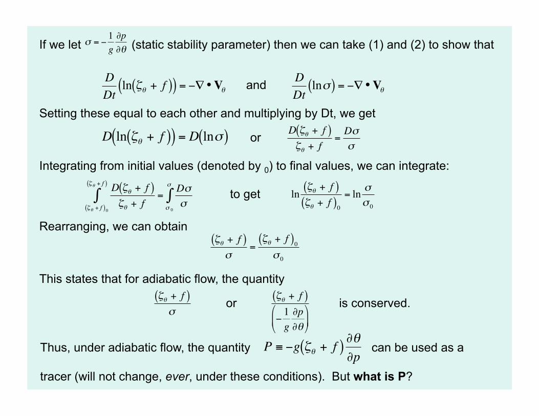
If we let (static stability parameter) then we can take (1) and (2) to show that

!

" = #1g$p$%

!

DDt

ln "# + f( )( ) = $% •V# and

Setting these equal to each other and multiplying by Dt, we get

!

D ln "# + f( )( ) = D ln$( ) or

!

D "# + f( )"# + f

=D$$

Integrating from initial values (denoted by 0) to final values, we can integrate:

!

D "# + f( )"# + f"# + f( )0

"# + f( )

$ =D%%% 0

%

$

!

ln"# + f( )"# + f( )0

= ln $$ 0

to get

!

"# + f( )$

="# + f( )0$ 0

Rearranging, we can obtain

This states that for adiabatic flow, the quantity

!

"# + f( )$

!

"# + f( )

$1g%p%#

&

' (

)

* +

or is conserved.

!

P " #g $% + f( ) &%&p

Thus, under adiabatic flow, the quantity can be used as a

tracer (will not change, ever, under these conditions). But what is P?

Isentropic Potential Vorticity

•  Following the motion, IPV will be conserved under adiabatic conditions (i.e. no mixing/friction, diabatic effects). If one parameter changes, then the others must adjust.

•  Called PV because there is the “potential” for generating vorticity by changing latitude or changing stability.

•  Since is negative for synoptic scale motions, PV is positive.

•  For synoptic scale motions, so

!

P = "g #$ + f( ) %$%p

!

"# =$v$x

+$u$y

%

& '

(

) * #

isentropic potential vorticity

(or Ertel’s PV)

relative vorticity

calculated on

isentropic surface

“earth’s” vorticity (latitude

dependent)

lapse rate of potential temperature

where

!

"#"p

!

"#"p

$ %10 K

100 hPa

!

P = " 10 m s-2( ) 10"4 s-1( ) " 10 K100 hPa

#

$ %

&

' (

1 hPa105 kg m s-2 m-2

#

$ %

&

' (

P =10"6m2 s-1 K kg-1 )1 PVU PVU = potential vorticity unit

!

P = "g #$ + f( ) %$%pImplications of IPV conservation

!"

! + d!"p

-dp

! + d!"

!"

-dp p

Convergence/Divergence ! Change relative vorticity (keeping latitude fixed) ! Change stability

Parcel changes latitude ! Change f and absolute vorticity (keeping stability constant) ! Change relative vorticity

Under constant stability, parcels moving south (north) will increase (decrease) in relative vorticity.

Under constant relative vorticity, parcels moving south (north) will increase (decrease) in stability.

IPV “Invertibility” •  One advantage of IPV thinking is that it is invertible - that is - if the

distribution if IPV(x,y,p) is known, then you know a lot about the distribution of !, u, v

•  The vorticity field tells you u and v as a function of x and y •  The static stability tells you about the vertical distribution of ! and

thus T •  The hydrostatic equation and the T field allows you to calculate the

distribution of #"•  Knowing # and u and v allows you to diagnose Vag, and thus $"•  However, you need to know more than just the IPV distribution to

actually calculate all of the above. In other words, you need to know how to relate the vorticity and static stability information, as well as know what the values are since the same IPV value can be reached with a number of combinations of vorticity and static stability.

•  This can be done given the following: 1.  The distribution of IPV is known 2.  The boundary conditions of the domain 3.  A balance condition can be applied that relates the mass and

momentum fields within the domain (e.g. geostrophic or gradient wind balance)

Values of IPV < 1.5 PVU are generally associated with tropospheric air

Values of IPV > 1.5 PVU are generally associated with stratospheric air

Fig. 1.137 Bluestein vol II

Globally averaged IPV in January

Note position of IPV = 1.5 PVU (red contour)

350 K isentrope pressure varies little with latitude, although it is in the stratosphere at high latitudes, and in the troposphere at low latitudes

300 K isentropic surface slopes much more, usually located in troposphere

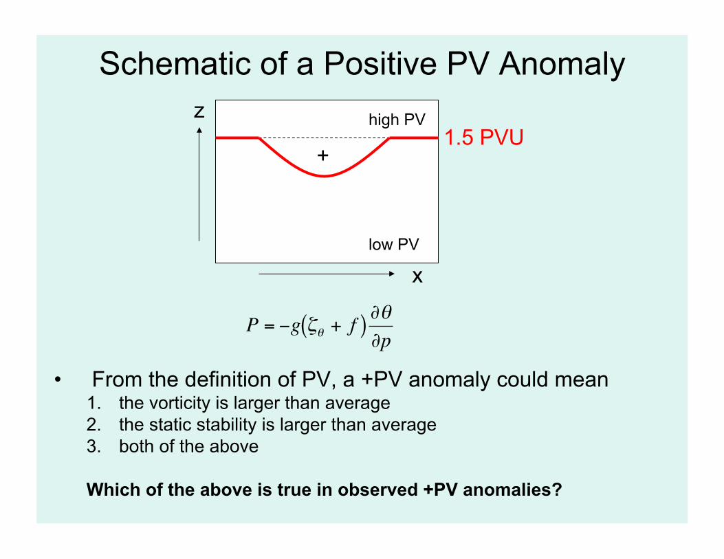
Schematic of a Positive PV Anomaly

•  From the definition of PV, a +PV anomaly could mean 1.  the vorticity is larger than average 2.  the static stability is larger than average 3.  both of the above

Which of the above is true in observed +PV anomalies?

z

x

1.5 PVU +

high PV

low PV

!

P = "g #$ + f( ) %$%p

Vertical Structure of a + IPV anomaly

Martin (2006) p. 281

In order to answer this question, let’s think of the structure of the atmosphere near a +PV anomaly

Imagine a +PV anomaly is completely resultant from a vorticity anomaly in thermal wind balance

Since the PV anomaly is is maximized in the upper troposphere, the winds must be maximized at that level.

Thus the winds must be increasing with height.

!

VT ="Vg

"p=

ˆ k f#$

"%"p

Vertical Structure of a + IPV anomaly

Given thermal wind balance, this implies that a relatively cold column of air must reside directly under the PV anomaly, with warm air surrounding it.

Martin (2006) p. 281 !

VT ="Vg

"p=

ˆ k f#$

"%"p

Vertical Structure of a + IPV anomaly

In the stratosphere above the +PV anomaly, due to thermal wind balance there must be warm air above the +PV anomaly, and cold air surrounding it.

Martin (2006) p. 281 !

VT ="Vg

"p=

ˆ k f#$

"%"p

Vertical Structure of a + IPV anomaly

Martin (2006) p. 281

Placing the isentropes in the figure answers our question: The +PV anomaly is represented by both a positive vorticity anomaly and a positive static stability anomaly.

IPV anomalies: kinematic and thermal structure

z

x

1.5 PVU +

high PV

low PV

z

x

-

high PV

low PV

!"

!+%!"

!+2%!"

!"

!+%!"

!+2%!"

A +PV anomaly has isentropic surfaces which bow towards the anomaly both in the troposphere and the stratosphere ! increased static stability

A -PV anomaly has isentropic surfaces which bow away the anomaly both in the troposphere and the stratosphere ! decreased static stability

"

"

"

#

#

#

#

#

#

"

"

"

Positive PV Anomaly Negative PV Anomaly

(into page) (out of page)

Gradients in PV are where the action occurs - jets, steep stability gradients, and tropopause “folds”

Cross section through a + UL IPV anomaly

Cross section through a – UL IPV anomaly

Positive PV Anomalies and Cyclogenesis

1.5 PVU +

!"

!+%!"

!+2%!"

!-%!"

z

x +$ -$

Suppose a traveling +PV anomaly crosses an area from west to east.

Isentropes must deform so as to take on the structure of a +PV anomaly.

Thus, adiabatic flow in a system-relative sense will enter the region of the +PV anomaly from the east and depart to the west.

The flow will follow the isentropes barring any diabatic effects, and will undergo isentropic upglide on the east side of the system, and isentropic downglide on the west side of the system.

Does this sound familiar?

Recall that the QG height tendency equation (ignoring friction and diabatic heating) is:

We can rewrite this as:

If we add d(ff0)/dt = 0 to the LHS of the equation we obtain:

Dividing both sides by f0 we obtain:

Relation between QG theory and IPV thinking

!

"2 +f02

#$2

$P 2

%

& '

(

) * $+$t

= , f0 V g •"1f0"2++ f

%

& '

(

) *

-

. /

0

1 2 +

f02

#$$P

,V g •"$+$P

%

& '

(

) *

!

""t

#2$+f02

%"2$"P 2

&

' (

)

* + = , V g •# #2$+ ff0 +

f02

%"2$"P 2

&

' (

)

* +

-

. /

0

1 2

!

""t

#2$+ ff0 +f02

%"2$"P 2

&

' (

)

* + = , V g •# #2$+ ff0 +

f02

%"2$"P 2

&

' (

)

* +

-

. /

0

1 2

!

""t

1f0#2$+ f +

f0%"2$"P 2

&

' (

)

* + = , V g •#

1f0#2$+ f +

f0%"2$"P 2

&

' (

)

* +

-

. /

0

1 2 (1)

Now, we will define QG potential vorticity (PQG) as

So our equation (1) above now becomes:

If we take the total derivative of PQG we get:

With equation (2), then the following must be true:

Thus, the QG height tendency equation can be used to show that geostrophic PV is conserved following adiabatic geostrophic flow.

Relation between QG theory and IPV thinking (2)

!

PQG "1f0#2$+ f +

f0%&2$&P 2

!

""t

PQG( ) = # V g •$PQG[ ]

!

DPQGDt

=""t

PQG( ) +V g •#PQG

(2)

!

DPQGDt

= 0

Relation between QG theory and IPV thinking

1.5 PVU +

!"

!+%!"

!+2%!"

!-%!"

z

x +$ -$

Let’s return to this schematic.

In the region of depicted isentropic upglide, there is clearly positive PV advection. Equation (2) on the previous page requires that this region has to have a local increase in PV.

Equating , and with PQG increasing with time, then

will be positive and thus will be negative.

Thus the +PV anomaly will lead to height falls in this region of upward motion caused by adiabatic cooling in the ascending air.

!

""t

PQG( ) = # V g •$PQG[ ]

!

""t

PQG( ) # $2 +f02

%"2

"P 2

&

' (

)

* + ","t

!

"2 +f02

#$2

$P 2

%

& '

(

) * $+$t

!

"#"t

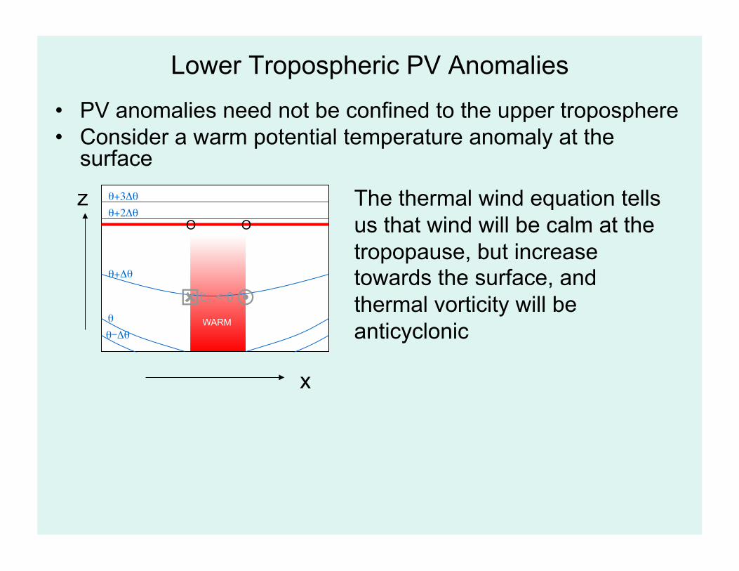
Lower Tropospheric PV Anomalies

•  PV anomalies need not be confined to the upper troposphere •  Consider a warm potential temperature anomaly at the

surface

z

x

!"

!+%!"

!+2%!"

!+3%!"

WARM

# " &T < 0

O O

The thermal wind equation tells us that wind will be calm at the tropopause, but increase towards the surface, and thermal vorticity will be anticyclonic !-%!"

Lower Tropospheric PV Anomalies

•  PV anomalies need not be confined to the upper troposphere •  Consider a warm potential temperature anomaly at the

surface

z

x

!"

!+%!"

!+2%!"

!+3%!"

WARM

# " &T < 0

O O

However, distribution of isentropes tells us that we have a +PV anomaly at the surface!

There is also a maximum in static stability near the surface if one considers connecting the isentropes below ground.

!-%!"

" # & > 0

Upper-level +PV’

Low-level +PV’

Vorticity conservation Temperature conservation

consistency with QG thinking

Bluestein’s thinking: assume a IPV anomaly-relative frame of reference the local PV (and abs vort) remain unchanged then look at the QG vort eqn

consistency with QG thinking

Bluestein’s thinking: assume a P’-relative frame of ref the P (and T) remain unchanged then look at the QG 1st law

consistency with QG thinking

consistency with QG thinking

!"

Propagation of Lower Tropospheric PV Anomalies Let us consider what happens at upper levels during cyclogenesis from the PV perspective.

Consider a + PV anomaly at initial time t. It will have a cyclonic circulation associated with it that will advect low PV air poleward and high PV equatorward.

+ t = 0

high PV

low PV x

y

Propagation of Lower Tropospheric PV Anomalies Let us consider what happens at upper levels during cyclogenesis from the PV perspective.

At a later time, the +PV anomaly will advect low PV air poleward, creating a -PV anomaly to the east.

The original anomaly will advect higher PV air equatorward, causing it to propagate west.

+ t = 0

high PV

low PV x

y

+ t = t+%t

high PV

low PV x

y -

Propagation of Lower Tropospheric PV Anomalies Let us consider what happens at upper levels during cyclogenesis from the PV perspective.

Subsequently, the original +PV anomaly continues to propagate westward while a secondary +PV anomaly is spawned to the east.

This analysis shows that upper level PV anomalies will tend to propagate westward, as long (Rossby) waves do through advection of planetary vorticity (f).

+ t = 0

high PV

low PV x

y

+ t = t+%t

high PV

low PV x

y -

+ t = t+%t x

y - +

high PV

low PV

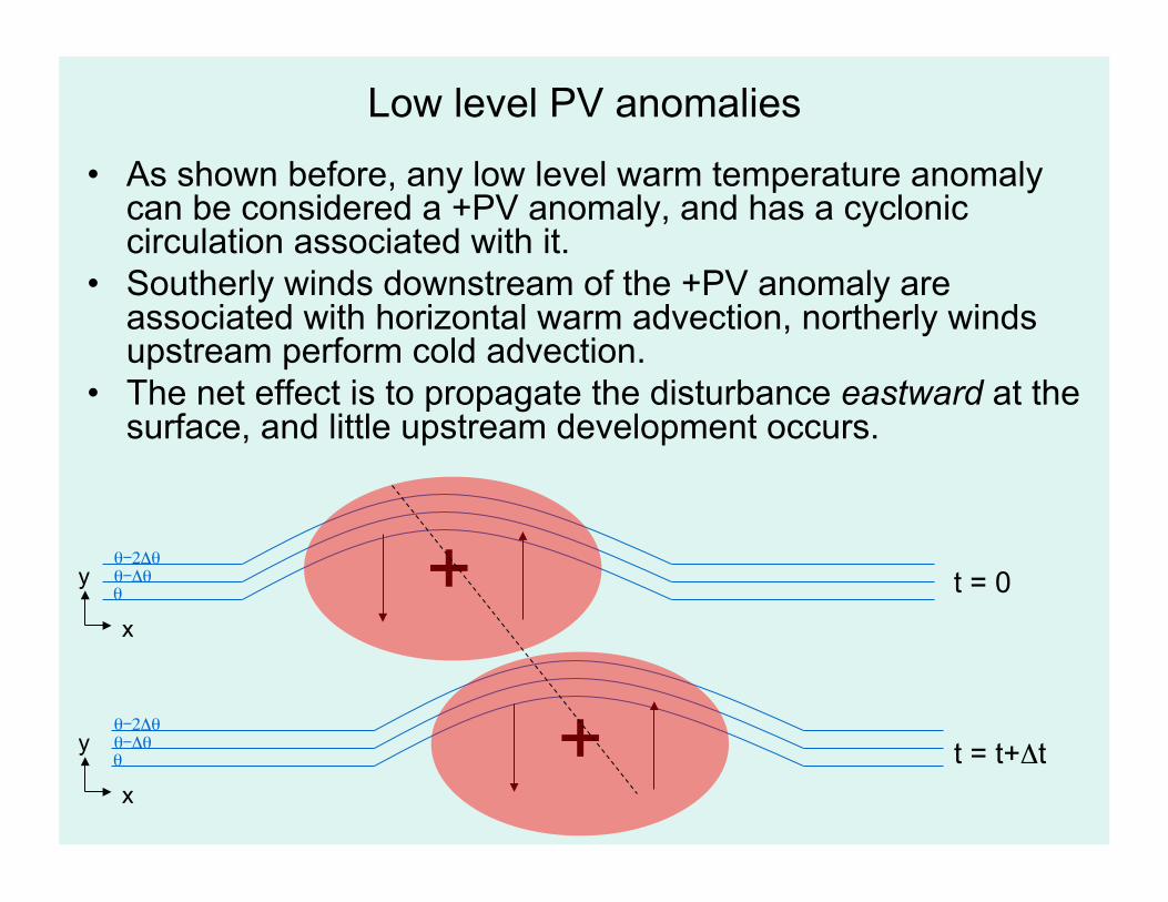
Low level PV anomalies

•  As shown before, any low level warm temperature anomaly can be considered a +PV anomaly, and has a cyclonic circulation associated with it.

•  Southerly winds downstream of the +PV anomaly are associated with horizontal warm advection, northerly winds upstream perform cold advection.

•  The net effect is to propagate the disturbance eastward at the surface, and little upstream development occurs.

!"!-%!"!-2%!"

!"!-%!"!-2%!"

+

+x

y

x

y

t = 0

t = t+%t

Lower and upper level PV anomalies together •  Through scale analysis, a PV anomaly will have a

“penetration depth” H of

•  For an anomaly 1000 km in horizontal dimension centered at 300 hPa, the vertical scale of a PV anomaly will be roughly enough amplitude to reach through most of the troposphere.

•  Thus, it is likely that –  an upper level PV anomaly can penetrate down to the surface and

contribute to the generation of a low level warm anomaly (through warm advection)

–  the circulation associated with a low level warm anomaly may extend far enough upward to cause horizontal PV advection at upper levels

•  So, given proper phasing, PV anomalies at different levels may amplify each other given the proper phasing.

!

H =fLN

L is the length scale of the anomaly

N is the Brünt-Vaisala Frequency

!

N =g"0

#"#z

!

H =10-4 s-1 1000 km

0.0129 s-1103m

km= 7752 m

!

N =10 m s-1

300 K5 Kkm

km103m

= 0.029 s-1

From the PV perspective, development of cyclones depends on a prolonged period of mutual

amplification of upper and lower level anomalies

However, we showed that upper level anomalies and lower level anomalies propagate like Rossby waves

in opposite directions

How does cyclogenesis occur in the PV world?

Cyclogenesis from the PV perspective

+

!"!-%!"!-2%!"

PV"PV+%PV"

Consider an upper tropospheric +PV anomaly moving over a surface baroclinic zone.

The upper level anomaly has a cyclonic wind anomaly, and extends throughout some depth of the troposphere, as determined by the penetration depth.

The influence of the upper level +PV anomaly is to deform the sea-level circulation through horizontal temperature advection.

t = 0

300 hPa

surface y

x

z

y

x

z

Cyclogenesis from the PV perspective

+

!"!-%!"!-2%!"

PV"PV+%PV"

The warm air advection acts on the surface isentropes to create a warm anomaly; this anomaly creates a circulation that penetrates the tropopause given by its penetration depth.

The surface warm anomaly will have a reflection on the 300 hPa field by inducing a cyclonic circulation that will strengthen the +PV anomaly through equatorward +PV advection on the east side of the PV anomaly.

This will cause the upper level PV anomaly to propagate eastward, contrary to its inclination to propagate westward.

t = %t

300 hPa

surface y

x

z

y

x

z

+

Cyclogenesis from the PV perspective

+

!"!-%!"!-2%!"

PV"PV+%PV"

The invigorated upper level anomaly exerts an invigorated influence on the low level isentrope field.

Since the upper level +PV anomaly lies upstream of the surface warm anomaly, this maximizes thermal advection where the maxima in warm anomalies where they already exist.

Thus the upper level +PV-induced warm and cold advection aid in strengthening the lower level +PV feature, and act together to allow the PV to propagate eastward.

t = 2%t

300 hPa

surface y

x

z

y

x

z

+

Cyclogenesis from the PV perspective

+

!"!-%!"!-2%!"

PV"PV+%PV"

Thus when upper and lower PV anomalies are in close proximity, they can mutually amplify, as well as ‘phase lock’ which allows them to propagate together.

Upshear (westward) tilt of the cyclone with height is a requisite condition for this process to occur, and thus it is benefical for systems to have upshear tilt for maximum intensification. (consistent with QG theory)

Also, it appears that cyclogenesis occurs independently of frontogenesis, which is why cyclones can form in the QG system despite the lack of fronts.

t = 2%t

300 hPa

surface y

x

z

y

x

z

+

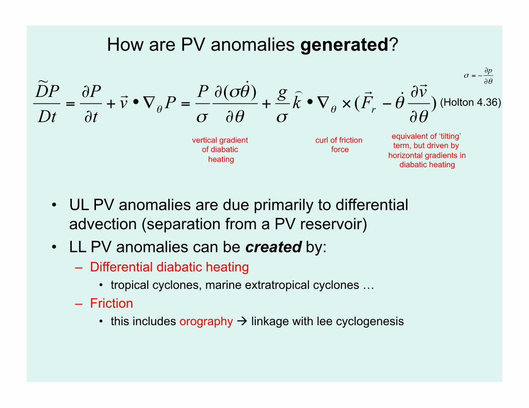
How are PV anomalies generated?

•  UL PV anomalies are due primarily to differential advection (separation from a PV reservoir)

•  LL PV anomalies can be created by: –  Differential diabatic heating

•  tropical cyclones, marine extratropical cyclones … –  Friction

•  this includes orography $ linkage with lee cyclogenesis

(Holton 4.36)

vertical gradient of diabatic

heating

equivalent of ‘tilting’ term, but driven by

horizontal gradients in diabatic heating

curl of friction force

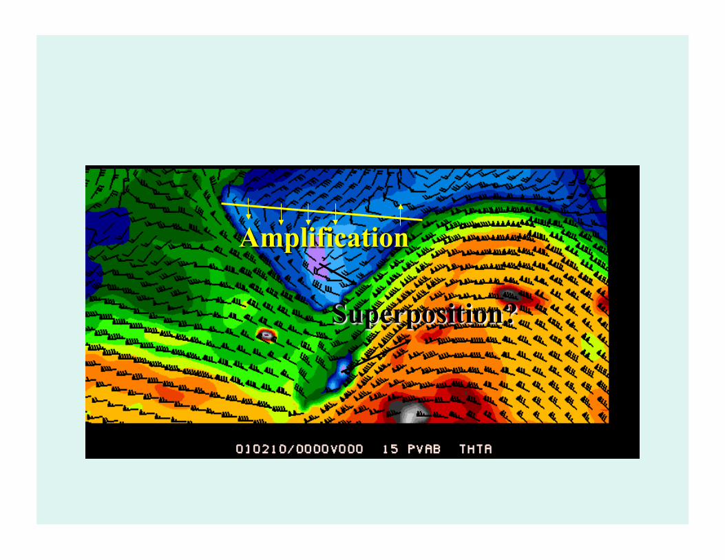
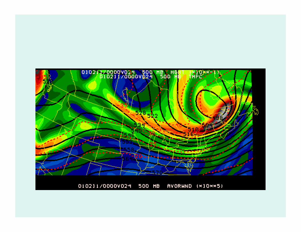
Predicting the change in time of PV anomalies •  Since the only way PV can change is through

advection (outside of mixing and diabatic effects), in a wave sense you can only change PV two ways: –  Increase the size of the PV anomaly

•  “Amplification” –  Increase the amount of PV (or number of PV anomalies)

within a small area •  “Superposition”

•  The following animations show IPV at the tropopause showing both of these effects, followed by a 500 hPa absolute vorticity loop of the same time period

(This animation is courtesy of John Nielsen-Gammon, Texas A&M University)

IPV and Terrain •  Can track systems over topography

–  Vorticity is altered by stretching and shrinking as parcels go over mountains

–  Potential vorticity is conserved on isentropic surfaces –  PV shows you what the trough will look like once it leaves

the mountains –  Better forecasts, better comparison with observations

Motion of low-level PV anomalies near a mountain range

In order to investigate PV on pressure surfaces instead of isentropic surfaces, we will derive an equation for the Lagrangian rate of change of PV. To do this, we will seek to first calculate expressions for the relative vorticity on isentropic coordinates

We can write differentials for u and v on constant theta surfaces as

Rearranging, we obtain

Now, let’s write down Poisson’s equation in a slightly varied form

We can also write Poisson’s equation in differential forms (& use ideal gas law)

PV on pressure surfaces

!

"# =$v$x%

& '

(

) * #

+$u$y%

& '

(

) * #

!

P = "g #$ + f( ) %$%p

!

du" = #u#x( )y,p dx" + #u

#y( )x,pdy" + #u

#p( )x,ydp"

dv" = #v#x( )y,p dx" + #v

#y( )x,p dy" + #v#p( )x,y dp"

!

dudy( )

"= #u

#y( )"

= #u#y( )

x,p+ #u

#p( )x,y

#p#y( )

"

dvdx( )" = #v

#x( )" = #v#x( )y,p + #v

#p( )x,y#p#x( )

"

(1)

(2)

!

p =1000 T"

#

$ % &

' (

c pR

!

dpdy( )

"= cp# dT

dy( )"

!

dpdx( )

"= cp# dT

dx( )"(3) (4)

we want an equation for this

We can also write down differential forms of T on an isentropic surface

Substituting from (3) and (4) we get

both of which have the same terms on the RHS, so we can set them equal to get:

If we take -'/'p, '/'x, and '/'y of the Poisson equation on a constant isobaric surface we get

!

dTdx( )" = #T

#x( )" = #T#x( )y,p + #T

#p( )x,y

#p#x( )

"

dTdy( )

"= #T

#x( )" = #T#y( )x,p + #T

#p( )x,y #T#y( )

"

(5)

(6)

!

1c p p

dpdx( )

"= #T

#x( )y,p + #T#p( )

x,y

#p#x( )

"

1c p p

dpdy( )

"= #T

#y( )x,p + #T#p( )x,y #T

#y( )"

!

dpdx( )

"= #T

#x( )y,p 1c p p

$ #T#p( )

x,y

% & '

( ) *

dpdy( )

"= #T

#y( )x,p

1c p p

$ #T#p( )

x,y

% & '

( ) *

!

" T#$#$p = 1

c p%" $T

$p( )T#

$#$x( )p = $T

$x( )pT#

$#$y( )

p= $T

$y( )p

(7)

(8)

so (7) & (8) become

!

dpdx( )

"= #"

#x#"#p

dpdy( )

"= #"

#y#"#p

(9)

(10)

Using (9) and (10) in (1) and (2) we can now say

Now we have what we want for calculating relative vorticity:

We know that . Substituting, and multiplying by g'!/'p

All the terms on the RHS involve pressure coordinates, so we can now (by adding f to both sides) make the statement that

So, PV is conserved on isobaric surfaces as well (vorticity balances (!) and can be evaluated on pressure surfaces as well as isentropic surfaces; however it is not as easy to evaluate (! on isobaric surfaces as it is '!/'p on isentropic surfaces.

!

"u"y( )

#= "u

"y( )x,p

+ "u"p( )

x,y"#"y

"#"p[ ]

"v"x( )# = "v

"x( )y,p + "v"p( )x,y "#

"x"#"p[ ]

(11)

(12)

!

"# = $v$x( )# % $u

$y( )#

= $v$x( )y,p % $u

$y( )x,p + $v$p( )x,y $#

$x$#$p[ ] % $u

$p( )x,y $#$y

$#$p[ ]

!

" p = #v#x( )p $ #u

#y( )p

(13)

!

"g #$#p %$ = "g #$

#p %$ " g #v#p

#$#x + g #u

#p#$#y

!

P = "g #$ + f( ) %$%p = "g f ˆ k +& '!

V h( ) •&$

Diabatic Effects on PV Taking the total derivative of the result on the previous slide with lots of

manipulation, it can be shown that

!

ddt

P( ) " #g $ + f( ) %%p

dQdt

&

' (

)

* +

PV is increased (decreased) where the vertical gradient of diabatic heating is positive (negative)

z

x p !

dQdt

> 0!

ddt

P( ) < 0

!

ddt

P( ) > 0

For diabatic heating in the mid-troposphere, this causes destruction of PV in the upper troposphere and creation of PV in the lower troposphere.

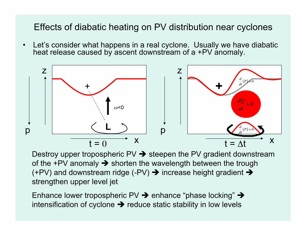
Effects of diabatic heating on PV distribution near cyclones •  Let’s consider what happens in a real cyclone. Usually we have diabatic

heat release caused by ascent downstream of a +PV anomaly.

z

x p

z

x p !

dQdt

> 0

!

ddt

P( ) > 0

+

L

$<0 !

ddt

P( ) < 0+

Destroy upper tropospheric PV ! steepen the PV gradient downstream of the +PV anomaly ! shorten the wavelength between the trough (+PV) and downstream ridge (-PV) ! increase height gradient ! strengthen upper level jet

Enhance lower tropospheric PV ! enhance “phase locking” ! intensification of cyclone ! reduce static stability in low levels

t = %t t = 0

Treble Clefs

cyclone matures and begins to occlude, diabatic heating in TROWAL ! PV destruction aloft

with negative PV advection ! formation of cut off low

initial development of “open wave” cyclone

A “Treble Clef” pattern in the PV field is often observed with mature cyclones

t = %t

t = 2%t

t = 0

Martin (2006) p. 300-301

Water Vapor Imagery and PV

•  (IDV Demonstration)

Tropopause Folds & Upper Level Fronts

A

A’

B

B’

Forget PV! The Traditional Geopotential Height Maps Work

Fine! Advantages of Height

•  Identification and assessment of features

•  Inference of wind and vorticity

•  Inference of vertical motion?

Disadvantages of Height

•  Gravity waves and topography

•  Inference of evolution and intensification

•  Role of diabatic processes is obscure

•  Need 300 & 500 mb

What’s PV Got that Traditional Maps Haven’t Got?

Advantages of PV •  PV is conserved •  PV unaffected by

gravity waves and topography

•  PV at one level gives you heights at many levels

•  Easy to diagnose Dynamics

Disadvantages of PV •  Unfamiliar •  Not as easily available •  Not easy to eyeball

significant features •  Qualitative inference of

wind and vorticity •  Hard to diagnose

vertical motion?