INVESTIGATING THE LONG TERM CAUSAL ...* Associate Professor, School of Management Studies, Anna...

* Assistant Professor, Sri Ramalinga Sowdambigai College of Science and Commerce, Coimbatore.** Associate Professor, School of Management Studies, Anna University Regional Centre, Coimbatore.

INVESTIGATING THE LONG TERM CAUSALRELATIONSHIP AMONG MACRO ECONOMICVARIABLES AND LEADING STOCK MARKET

INDICES OF INDIA

1Manju K. V. and 2M. V. Subha

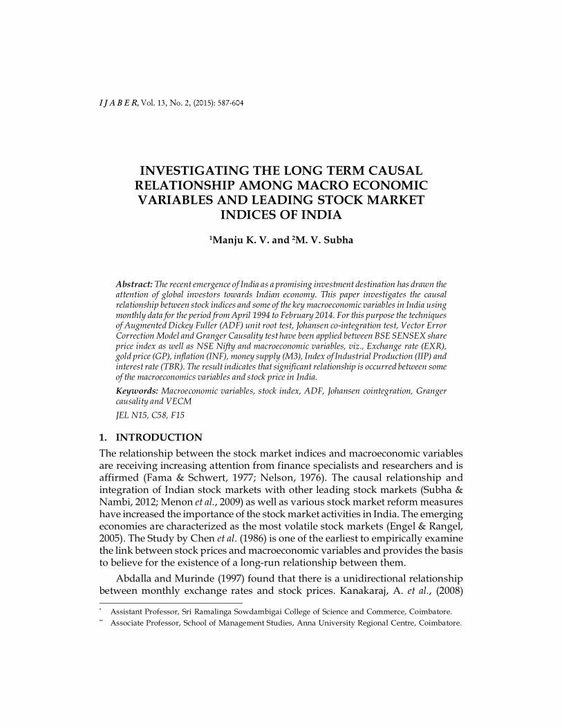
Abstract: The recent emergence of India as a promising investment destination has drawn theattention of global investors towards Indian economy. This paper investigates the causalrelationship between stock indices and some of the key macroeconomic variables in India usingmonthly data for the period from April 1994 to February 2014. For this purpose the techniquesof Augmented Dickey Fuller (ADF) unit root test, Johansen co-integration test, Vector ErrorCorrection Model and Granger Causality test have been applied between BSE SENSEX shareprice index as well as NSE Nifty and macroeconomic variables, viz., Exchange rate (EXR),gold price (GP), inflation (INF), money supply (M3), Index of Industrial Production (IIP) andinterest rate (TBR). The result indicates that significant relationship is occurred between someof the macroeconomics variables and stock price in India.

Keywords: Macroeconomic variables, stock index, ADF, Johansen cointegration, Grangercausality and VECM

JEL N15, C58, F15

1. INTRODUCTION

The relationship between the stock market indices and macroeconomic variablesare receiving increasing attention from finance specialists and researchers and isaffirmed (Fama & Schwert, 1977; Nelson, 1976). The causal relationship andintegration of Indian stock markets with other leading stock markets (Subha &Nambi, 2012; Menon et al., 2009) as well as various stock market reform measureshave increased the importance of the stock market activities in India. The emergingeconomies are characterized as the most volatile stock markets (Engel & Rangel,2005). The Study by Chen et al. (1986) is one of the earliest to empirically examinethe link between stock prices and macroeconomic variables and provides the basisto believe for the existence of a long-run relationship between them.

Abdalla and Murinde (1997) found that there is a unidirectional relationshipbetween monthly exchange rates and stock prices. Kanakaraj, A. et al., (2008)

I J A B E R, Vol. 13, No. 2, (2015): 587-604

588 � Manju K. V. and M. V. Subha

examined the trend of various macro economic variables and stock prices andconcluded by that there exists a strong relationship. Aman Srivastava (2010) foundthat interest rate, industrial production and wholesale price index influence theIndian stock market in the long run.

The Indian capital market has developed as an important source of raisingresources for Indian corporate. Currently, global investors and market participantsare vigilantly looking out the trends of Indian stock markets. Studying the causalrelationship between stock market indices and macroeconomic variables can beuseful for investors, traders and policy shapers.

The present paper attempts to analyze the long run relationship between BSESENSEX, NSE Nifty and macroeconomic variables like exchange rate, moneysupply, index of industrial production, gold price, interest rate and inflation duringthe post liberalisation period of 20 years 1994 to 2014.

2. REVIEW OF LITERATURE

The literature review shows that various studies have been conducted to learnabout the interrelationship between macroeconomic variables and stock marketindices. Ma and Kao (1990) examined the stock price reactions to exchange ratechanges and found that stock price is related to exchange rate changes. In a studyon the causal relationship between the U.S. stock market (S&P 500 index) andexchange rate of dollar in the short period of time, Bahmani and Sohrabian (1992)found bidirectional causality between the two for the studied time period, but,there was no long run relationship between the two variables. Ajayi and Mougoue(1996) in their study used daily data for eight countries to find interactions betweenstock markets and foreign exchange rates. A study conducted on the cause andeffect relationship between exchange rates and stock prices using daily marketdata by Pan, et al. (2001) showed that exchange rates Granger cause stock prices,but stock prices does not Granger cause exchange rate.

Various researches (Chen, Roll & Ross, 1986; Bodie, 1976; Fama, 1981; Geske &Roll, 1983; Pearce & Roley, 1983; James et al., 1985) have been conducted to establishempirical association between macroeconomic variables and stock market returns.Fama (1981), Geske and Roll (1983) and Pearce and Roley (1983) found a negativerelationship between stock market returns and inflation and money growth intheir studies. Chang and Pinegar (1989) in a study found that there is a closerelationship between the stock market and domestic economic activity. Malliarisand Urrutia (1991) observed that the performance of the stock market might beused as a leading indicator for real economic activities in the United States. In UKmarkets, Thornton (1993) found that stock returns tend to lead real income.Mukherjee and Naka (1995) carried out a study between the Japanese industrialproduction and stock market return and their study found a positive impact ofindustrial production growth on stock market return.

Investigating the Long term Causal Relationship among Macro Economic... � 589

Humpe and Macmillan (2009) conducted a study to relate the macro economicvariables with long term stock market movements in the US and Japan by usingmonthly data over 40 years. A cointegration analysis found significant relationbetween the macro economic variables namely, long term interest rates, moneysupply, industrial production, the consumer price index and stock prices in USand Japan.

Chakradhara Panda, et al., (2001) explored the interrelationship between realactivity, monetary policy, expected inflation and stock market returns in the postliberalization period using a vector – autoregression (VAR) approach. They foundout that no relationship exists between expected inflation and real activity. Expectedinflation as well as real activity influence stock returns. Bhattacharya and Mukherjee(2002) in their research found that there does not exist any relationship betweenthe stock prices and various macroeconomic aggregates such as national income,money supply and interest rates in India, but, there was a bi directional causationbetween inflation rate and stock prices.

Pal and Mittal (2011) examined the long run relationship between the IndianCapital Markets and key macroeconomic variables for the period from Jan 1995to Dec 2008. Their investigation found out that inflation and exchange rate havea significant impact on BSE SENSEX but influence of interest rate and grossdomestic saving (GDS) were insignificant. The relationships between Indian stockmarket index (BSE SENSEX) and money supply, industrial production index,treasury bills rates, wholesale price index and exchange rates was studied byPramod Kumar Naik and Puja Padhi (2012) wherein a positive relation betweenthe stock prices and money supply and industrial production was observed. Itwas observed that stock prices have a negative relation to inflation. Patel (2012)investigated the effect of macroeconomic determinants on the performance ofthe Indian Stock Market using monthly data over the period of 10 years (January1991 to December 2011). A long-run equilibrium relationship betweenmacroeconomic variables and the stock market index was observed by PramodKumar Naik (2013). Their study found positive relation among stock price,money supply and industrial production. Sangmi and Hassan (2013) examinedthe effect of macroeconomic variables on the stock price indices (BSE and NSE)for the period of four years (April 2008 to June 2012) using multiple regressionanalysis.

3. RESEARCH QUESTIONS

Recently, with relaxation in FDI norms to boost investor sentiments, India hasemerged as the most attractive investment destination. The literature review revealsthat until recently, a negligible amount of research has been conducted on Indianstock market and economic factors and thus the conclusion might be inadequate.Research which takes into consideration both BSE and NSE indices in the post


liberalisation period is minimal. The present paper is an attempt to fill this gap inthe literature.

Various studies regarding the interaction of share market returns and themacroeconomic variables provide different conclusions related to their test andmethodology. The results vary from market to market; may change in differentsample periods and also in different frequency of the data. Thus, more in-depthstudies are needed to understand the macroeconomic variables that might influencethe stock market in an emerging economy like India since it is one among thefastest growing economies.

Nearly two decades of economic liberalization, along with robust domesticdemand, a growing middle class, a young population, and a high return oninvestment make India a credible investment destination. Thus a study of postliberalization period of 20 years (1994 – 2014), considering both BSE and NSEwill be more useful to understand the long run relationship of macroeconomicvariables and stock markets effectively. As far as the developing countrylike India is concerned, the findings of this study would extend the existingliterature by providing some meaningful insight to the policy makers and theforeign investors.. The following are the two research questions considered inthis study:

1. Do macro economic variables influence leading stock indices of India?

2. Is there a long run causal relationship between economic variables andleading stock indices of India?

4. DATA

In this paper the relationship between stock market indices and six macroeconomicvariables are examined. The share price indices, BSE SENSEX (BSE) and NSE Nifty(NSE) represents the leading stock markets. The macroeconomic variablesconsidered for this study are exchange rate, (EXR), money supply (M3), the Indexof Industrial Production (IIP), gold price (GP), interest rate measured in terms ofImplicit Yield at Cut-off Price of 91 day Treasury bill rates (TBR) and inflation(INF). The period of study has been chosen as April 1994 to February 2014 since itrepresents the post liberalization period.

Monthly series for the period of 20 years (April 1994 to Feb 2014) wasconsidered which comprises 239 data points. The data for BSE and NSE historicalindices, exchange rate, money supply, index of industrial production, gold priceand interest rate has been compiled from the RBI Bulletin. Monthly All IndiaConsumer Price Index was collected from the website of Labour Bureau,Government of India. Table 1 shows a brief description of variables consideredfor this study.


Table 1Brief description of variables

Variable Definition of variables

LBSE Logarithms of Monthly average of BSE Sensitive IndexLNSE Logarithms of Monthly average of S&P CNX NIFTY IndexLEXR Logarithms of Monthly Average of exchange rate of Indian Rupee against US

DollarLM3 Logarithms of monthly values of M3LIIP Logarithms of monthly Values of IIPLGP Logarithms of Monthly average of Gold PriceTBR Average of weekly cut-off rate of 91 days treasury bills has been calculated to

obtain monthly valuesINF Point to Point Rate of Inflation in Consumer Price Index Numbers

5. METHODOLOGY

Based on the above discussion, the present study tries to investigate the long runrelationship between the stock price indices and six macro economics variables.For doing empirical analysis, two leading stock indices of India i.e., BSE Sensex(BSE) and NSE Nifty (NSE) have been considered as the dependent variables. Sothe following empirical models are estimated.

Xt = (LOGBSEt, EXRt, LOGM3t, LOGIIPt, LOGGPt, TBRt, INFt)

Yt = (LOGNSEt, EXRt, LOGM3t, LOGIIPt, LOGGPt, TBRt, INFt)

Where,

LOGBSE and LOGNSE are the stock market indices, EXR is the exchange rate-USD vs INR, LOGM3 is money supply, LOGIIP is the Index of IndustrialProduction, LOGGP is the gold price, TBR is interest rate measured in terms ofImplicit Yield at Cut-off Price of 91 day treasury bill rates, and INF is inflationmeasured in terms of Consumer Price Index- (CPI)

X and Y are 7×1 vector of variables.

5.1. Vector Error Correction Model

Vector Error Correction Model (VECM) is used in order to study the causal nexusbetween stock indices and macroeconomic variables in India.

i. The first step in estimating VECM is to pre-test for unit roots. It is used toexamine whether the data series are non-stationary. Augmented DickeyFuller Test (ADF) is used for this purpose.

ii. If the data series are stationary and of the same order, then, Johansen andJuselius (1990) multivariate co-integration technique is employed to


investigate the long run relationship between stock indices andmacroeconomic variables in India.

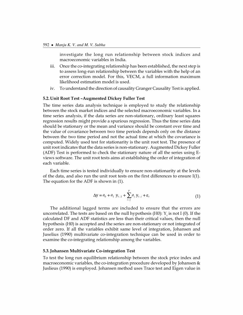
iii. Once the co-integrating relationship has been established, the next step isto assess long-run relationship between the variables with the help of anerror correction model. For this, VECM, a full information maximumlikelihood estimation model is used.

iv. To understand the direction of causality Granger Causality Test is applied.

5.2. Unit Root Test –Augmented Dickey Fuller Test

The time series data analysis technique is employed to study the relationshipbetween the stock market indices and the selected macroeconomic variables. In atime series analysis, if the data series are non-stationary, ordinary least squaresregression results might provide a spurious regression. Thus the time series datashould be stationary or the mean and variance should be constant over time andthe value of covariance between two time periods depends only on the distancebetween the two time period and not the actual time at which the covariance iscomputed. Widely used test for stationarity is the unit root test. The presence ofunit root indicates that the data series is non-stationary. Augmented Dickey Fuller(ADF) Test is performed to check the stationary nature of all the series using E-views software. The unit root tests aims at establishing the order of integration ofeach variable.

Each time series is tested individually to ensure non-stationarity at the levelsof the data, and also run the unit root tests on the first differences to ensure I(1).The equation for the ADF is shown in (1).

0 1 1

p

t j t i ti j

y a a y a y (1)

The additional lagged terms are included to ensure that the errors areuncorrelated. The tests are based on the null hypothesis (H0): Yt is not I (0). If thecalculated DF and ADF statistics are less than their critical values, then the nullhypothesis (H0) is accepted and the series are non-stationary or not integrated oforder zero. If all the variables exhibit same level of integration, Johansen andJuselius (1990) multivariate co-integration technique can be used in order toexamine the co-integrating relationship among the variables.

5.3. Johansen Multivariate Co-integration Test

To test the long run equilibrium relationship between the stock price index andmacroeconomic variables, the co-integration procedure developed by Johansen &Juslieus (1990) is employed. Johansen method uses Trace test and Eigen value in


order to find out the number of co-integrating relationships that may exist betweenthe variables. If the hypothesis that there is no co-integration is rejected, then astable long run relationship between stock index and related variable does exist.The Johansen’s estimation model is shown in equation (2).

p

t i t i t i tr j

X µ r X X (2)

where,

�Xt = (n × 1) vector of all the non-stationary indices in our study.

�t = (n × n) vector matrix of coefficients

� = (n × r) matrix of error correction coefficients where r is the number ofcointegrating relationships in the variables, so that 0 < r < n. This measures thespeed at which the variables adjust to their equilibrium. (Also known as theadjustment parameter)

� = (n × r) matrix of r cointegrating vectors, so that 0 < r < n. This is whatrepresents the long-run cointegrating relationship between the variables.

5.4. Vector Error Correction Model

A vector error correction model is a restricted VAR that has co-integrationrestrictions built into the specification. It is designed for use with non-stationaryseries that are known to be co-integrated. It also allows examining the causality inthe Granger sense. The significance of the lagged error correction term(s) indicatesthe long term Causal relationship. The cointegration term is known as errorcorrection term as the deviation from long-run equilibrium is corrected graduallythrough a series of partial short run adjustments. If two endogenous variables Y1tand Y2t have no trend and the cointegration equations (3) and (4) have an intercept,the VECM has the form

1 1 2, 1 1, 1 1,) )t t t tY Y µ Y (3)

2 2 2 , 1 1, 1 2 ,( )t t t tY Y µ Y (4)

5.5. Granger Causality Test

The causality relationships among the variables in this study are determined byusing the methodology based on Granger (1988). The Granger tests estimation iscarried out using the equations (5) and (6).

0 1 2 11 1

k m

t s t s i t m ts i

X X Y (5)


0 1 2 21 1

pn

t j t j h t h tj h

Y Y X (6)

where,

�1t and �2t are assumed to be uncorrelated and E(�1t �1s ) = E(�2t �2s) for all s � t.

These equations can be used to show the unidirectional causality from stockprice index and macroeconomic variables. If the estimated coefficients �21 arestatistically significant. i.e., �21 � 0, then Y Granger causes X. Similarly, if �2h isstatistically significant, i.e., �2h � 0, then X is the cause variable for Y. If both �21 and�2h are significant, there is a mutual dependency between these variables. If both�21 and �2h are statistically insignificant, then X and Y are independent.

6. EMPIRICAL RESULTS

6.1. Descriptive Statistics

Table 2 indicates that the mean and median of BSE, NSE, M3, IIP, GP, TBR andINF are equal. The values of standard deviation shows that EXR, TBR and INF aremore volatile compared to BSE, NSE, M3, IIP and GP. But the values of skewnessand kurtosis points towards lack of symmetry in data. The observed distributionis said to be normally distributed if the value of skewness and kurtosis are 0 and 3respectively. The significant coefficient of Jarque-Bera statistics also indicates thatthe considered series do not have normal frequency distribution. In other words itcan be said that there is no randomness in data and stands sensitive to speculationand periodic changes. This means that there is scope for the individual investorsto earn higher rate of profit by investing in Indian Stock Market. It also bringsforth the issue of inefficiency of the market.

Table 2Descriptive Statistics

LOGBSE LOGNSE EXR LOGM3 LOGIIP LOGGP TBR INF

Mean 3.848994 3.328863 44.28817 4.315914 2.316631 3.912612 7.428073 7.54477Median 3.734261 3.227007 44.9491 4.302256 2.295567 3.777172 7.332 7.71Maximum 4.321673 3.795662 63.65 4.971345 2.599791 4.500687 12.9672 19.7Minimum 3.457186 2.921784 31.3705 3.650146 1.999565 3.601517 3.22652 0Std. Dev. 0.310491 0.308088 6.668553 0.392027 0.168064 0.294212 2.224257 3.45773Skewness 0.272934 0.259713 0.168214 0.031104 0.015863 0.793057 0.446404 0.452306Kurtosis 1.374484 1.386021 3.604283 1.792477 1.675209 2.146488 3.113794 3.079762Jarque-Bera 29.28022 28.62754 4.763495 14.55889 17.48762 32.3072 8.066812 8.212476Probability 0 0.000001 0.092389 0.00069 0.000159 0 0.017714 0.01647Sum 919.9095 795.5982 10584.87 1031.503 553.6747 935.1144 1775.309 1803.2Observations 239 239 239 239 239 239 239 239


6.2. Correlation

The correlations between the stock variables for the period of April 1994 to February2014 are computed to measure the strength of association between the variables.The simple correlation coefficients among the 8 variables under study are given inTable 3.

Table 3Correlation Matrix

LOGBSE LOGNSE EXR LOGM3 LOGIIP LOGGP TBR INF

LOGBSE 1LOGNSE 0.998662 1EXR 0.521973 0.544731 1LOGM3 0.907556 0.920743 0.78457 1LOGIIP 0.928182 0.937937 0.712579 0.986345 1LOGGP 0.916567 0.919673 0.646657 0.918079 0.908781 1TBR -0.22474 -0.24586 -0.3114 -0.37998 -0.36267 -0.1285 1INF 0.27292 0.249786 -0.05949 0.143515 0.161216 0.382863 0.208745 1

While the numerical values of correlation coefficients may range from 1.0 to -1.0, the table shows very high positive correlation between most of the variablesunder consideration. It indicates that M3, IIP and GP are highly positively correlatedwith BSE and NSE. These high correlation also points towards multi-collinearityamong the variables. But correlation coefficients of EXR and INF are relativelyless and TBR shows negative correlation coefficients.

6.3. Unit Root Test – Augmented Dickey Fuller Test

The Augmented Dickey Fuller (ADF) test is employed to test the stationarity ofBSE, NSE, EXR, M3, IIP, GP, TBR and INF. The results on levels and first differenceare presented in Table 4.

Table 4Results of ADF test for unit root

ADF (Augmented Dickey Fuller) Test

Variables Levels First Difference

LOGBSE -2.371602 -12.07674LOGNSE -2.621825 -12.05992EXR -1.664104 -11.21026LOGM3 -2.107483 -11.49666LOGIIP -1.887318 -15.65948LOGGP -1.610327 -14.44060TBR -1.852039 -13.70494INF -3.382126 -10.48729


The critical values for unit root tests at 1%, 5% and 10% significance levels are-3.99,-3.42 and -3.13 (with trend) for ADF. The null hypothesis of ADF test is thatthe series has a unit root. If the absolute test statistics is more than the criticalvalue we can reject the null hypothesis. This means that the series is stationary.The results of ADF test indicate that there is the presence of unit root in the levelsof all variables. Therefore, the null hypothesis that the variables under study havea unit root cannot be rejected. This means that the variables are non-stationary.But in the first difference of all the variables there is no evidence for unit root. Thevalues are significant at 1% level. So the null hypothesis can be rejected and thevariables are stationary and integrated of order I(1). In this case we can use Johansenmultivariate co-integration test to see whether these variables are co-integrated.

6.4. Co-integration test results - Johansen test - BSE and macroeconomic variables

Johansen multivariate co-integration test is used in this study to determine whetherselected macroeconomic variables are co-integrated (hence possibly causallyrelated) with stock index (BSE SENSEX) in the long run.

The Trace Test results in Table 5 indicate that there exists one cointegratingequation at 5% level. This implies that one linear combination exists betweenvariables that force these variables to hold a relationship over the entire time period,despite potential deviations from equilibrium levels in the short-run.

Table 5Results of trace test - Johansen co-integration - LOGBSE and the macroeconomic variables

Series: LOGBSE EXR LOGM3 LOGIIP LOGGP TBR INF Unrestricted Cointegration Rank Test (Trace)

Hypothesized Trace 0.05 Prob.**No. of CE(s) Statistic Critical Value

None * 157.7791 125.6154 0.0001At most 1 87.98840 95.75366 0.1518At most 2 57.38217 69.81889 0.3244At most 3 33.74380 47.85613 0.5159At most 4 18.09924 29.79707 0.5587At most 5 4.239996 15.49471 0.8832At most 6 0.173929 3.841466 0.6766

Trace test indicates 1 cointegrating eqn(s) at the 0.05 level* denotes rejection of the hypothesis at the 0.05 level** MacKinnon-Haug-Michelis (1999) p-values

The results of the Maximum Eigen Value test in Table 6 can be analysed so asto confirm the results of the Johansen’s Trace test.


Table 6Johansen co-integration results – max-eigen value test - LOGBSE and the

macroeconomic variablesUnrestricted Cointegration Rank Test (Maximum Eigenvalue)

Hypothesized Max-Eigen 0.05 Prob.**No. of CE(s) Statistic Critical Value


Max-eigenvalue test indicates 1 cointegrating eqn(s) at the 0.05 level* denotes rejection of the hypothesis at the 0.05 level** MacKinnon-Haug-Michelis (1999) p-values

The Maximum Eigen Value test also shows one cointegrating equation at 5%level confirming the Trace Test. Consequently a cointegrating relationship overthe 20 year sample period is confirmed.

Since we have identified the existence of one cointegrating equation, we cansay that a stable equilibrium relationship is present. A method of normalisation isrequired for cointegrated time series systems. The process of normalisation causesthe matrix to be consistant with the economic theory. The results are normalizedon LOGBSE as shown in Table 7.

Table 7Normalized cointegrating coefficients –LOGBSE and macroeconomic variables

Normalized cointegrating coefficients (standard error in parentheses)

LOGBSE EXR LOGM3 LOGIIP LOGGP TBR INF

1.000000 0.185758 -20.00722 32.90301 3.371628 -0.170697 -0.035113(0.02434) (2.30859) (3.98382) (0.92610) (0.04167) (0.02409)

6.5. Vector Error Correction Model - LOGBSE and Macroeconomic Variables

Assuming one co-integrating vector, long run interaction of the underlyingvariables the VECM has been estimated based on the Johansen cointegrationmethodology. The estimated co-integrating coefficients for the BSE SENSEX basedon the first normalized eigenvector can be expressed as:

Xt = (LOGBSEt, EXRt, LOGM3t,LOGIIPt, LOGGPt, TBRt, INFt)

B1 = (1.00, 0.18, -2.00, 32.90, 3.37, -0.17, -0.03)


These values represent the coefficient for BSE (normalized to one), EXR, M3,IIP, GP, TBR and INF. The signs are reversed so as to enable proper interpretationas a result of the normalization process. So the long-run equilibrium relationshipcan be re-expressed based upon the result of vector error correction model shownin Table 8.

Table 8Result of vector error correction model - LOGBSE and macroeconomic variables

LOGBSE(-1) EXR(-1) LOGM3(-1) LOGIIP(-1) LOGGP(-1) TBR(-1) INF(-1) C

1.000000 0.185758 -2.00722 32.90301 3.371628 -0.1707 -0.03511 -13.615 (0.02434) (2.30859) (3.98382) (0.92610) (0.04167) (0.02409)[ 7.63181] [-8.66641] [ 8.25917] [ 3.64069] [-4.09671] [-1.45765]

R-squared: 0.12Probability value of LM Test : 0.90Probability value of Heteroskedasticity Test : 0.36

LOGBSE = 2.00 LOGM3 - 0.18 EXR- 32.90 LOGIIP-3.37 LOGGP+ 0.17 TBR+ 0.03 INF +13.615

The coefficients for LOGM3, TBR and INF are positive and the coefficients forEXR, LOGIIP and LOGGP are negative. This means that LOGM3, TBR and INFhave a positive long- run relationship with LOGBSE, whereas EXR, LOGIIP andLOGGP have a negative relationship with LOGBSE.

The R squared value shows that only 12% of the variation in the stock priceindex is explained by exchange rate, money supply, index of industrial production,gold price, interest rate and inflation. The probability value of LM Test shows thatthere is no serial correlation in the model. The model does not haveheteroskedasticity as per the results.

6.6. Co-integration Test Results-Johansen Test – LOGNSE and MacroeconomicVariables

In order to examine whether selected macroeconomic variables are co-integratedwith stock index (NSE Nifty) in the long run, Johansen multivariate co-integrationtest is employed. Table 9 shows the trace test result of co-integration betweenLOGBSE and the macroeconomic variables. It provides the test statistics for co-integration and critical values at 5% level.

The Trace Test results in Table 9 indicate that there exists one co-integrating equation at 5% level. The results of the Maximum Eigen Value testin Table 10 can be analysed so as to confirm the results of the Johansen’s Tracetest.


Table 10Johansen co-integration results – max-eigen value test - LOGNSE and the

macroeconomic variablesUnrestricted Cointegration Rank Test (Maximum Eigenvalue)

Hypothesized Eigenvalue Max-Eigen 0.05 Prob.**No. of CE(s) Statistic Critical Value

None * 0.259603 70.93410 46.23142 0.0000At most 1 0.128145 32.36317 40.07757 0.2835At most 2 0.095529 23.69551 33.87687 0.4780At most 3 0.064437 15.71926 27.58434 0.6895At most 4 0.056112 13.62849 21.13162 0.3962At most 5 0.016430 3.909758 14.26460 0.8687At most 6 0.001147 0.270833 3.841466 0.6028

Max-eigenvalue test indicates 1 cointegrating eqn(s) at the 0.05 level* denotes rejection of the hypothesis at the 0.05 level** MacKinnon-Haug-Michelis (1999) p-values

The Maximum Eigen Value Test also shows one co-integrating equation at 5%level confirming the Trace Test. Consequently a co-integrating relationship overthe 20 year sample period is confirmed. Since there is one co-integrating equation,a stable equilibrium relationship is present. Now the normalized co-integratingcoefficient in the VECM can be analyzed as shown in Table 11.

Table 9Results of trace test - Johansen co-integration - LOGNSE and the macroeconomic

variablesSeries: LOGNSE EXR LOGM3 LOGIIP LOGGP TBR INF

Unrestricted Cointegration Rank Test (Trace)

Hypothesized Trace 0.05 Prob.**No. of CE(s) Statistic Critical Value


Trace test indicates 1 cointegrating eqn(s) at the 0.05 level* denotes rejection of the hypothesis at the 0.05 level** MacKinnon-Haug-Michelis (1999) p-values


Table 11Normalized co-integrating coefficients - NSE

Normalized cointegrating coefficients (standard error in parentheses)

LOGNSE EXR LOGM3 LOGIIP LOGGP TBR INF

1.000000 0.135496 -14.35179 23.23547 2.299292 -0.123400 -0.022569 (0.01707) (1.61823) (2.79166) (0.64832) (0.02911) (0.01689)

6.7. Vector Error Correction Model - LOGNSE and Macroeconomic Variables

As there is one co-integrating vector, the short run and long run interaction of theunderlying variables, the VECM has been calculated as per the Johansen co-integration methodology. The results show that a long-run equilibrium relationshipexists between the stock market indices and the macroeconomic variables. It isclear that there is one co-integrating vector or one error term as per Trace andMaximum Eigen value. The estimated co-integrating coefficients for the BSEsensitive index based on the first normalized eigenvector are as follows.

Yt = (LOGNSEt, EXRt, LOGM3t, LOGIIPt, LOGGPt, TBRt, INFt)

Bt = (1.00, 0.13, -14.35, 23.23, 2.29, -0.12, -0.02)

These values represent the coefficient for NSE (normalized to one), EXR, M3,IIP, GP, TBR and INF. Thus the long-run equilibrium relationship can be re-expressed on the basis of VECM results presented in Table 12.

Table 12Result of vector error correction model - LOGNSE and macroeconomic variables

LOGNSE(-1) EXR(-1) LOGM3(-1) LOGIIP(-1) LOGGP(-1) TBR(-1) INF(-1) C

1.000000 0.135496 -14.35179 23.23547 2.299292 -0.1234 -0.02257 -9.12935(0.01707) (1.61823) (2.79166) (0.64832) (0.02911) (0.01689)

[ 7.93769] [-8.86880] [ 8.32319] [ 3.54654] [-4.23901] [-1.33649]

R-squared : 0.11Heteroskedasticity Test : 0.40Probability value for LM Test : 0.91

LOGNSE = 14.35 LOGM3 – 0.13 EXR - 23.23 LOGIIP – 2.29 LOGGP + 0.1 2TBR + 0.02 INF + 9.12

The coefficients of the long run equation indicates LOGM3, TBR and INF havepositive relationship with LOGNSE and all the other macroeconomic variablesshow a negative relationship with LOGNSE. This result is consistent with that ofLOGBSE and macroeconomic variables. This means that LOGM3, TBR and INFhave a positive long run relationship with both BSE and NSE.

The R squared value shows that only 11% of the variation in the stock priceindex is explained by exchange rate , money supply,index of industrial


production, gold price, interest rate and inflation. The probability value ofLM test indicates that there is no serial correlation among the variables. Theresult of heteroskedasticity test shows that there is no heteroskedasticy in themodel.

6.8. Granger Causality Test

The co-integration results indicate that causality exists between the co-integratedvariables, however, it fails to show us the direction of the causal relationship.Granger causality enables us to identify the direction of causal relationshipbetween the stock price index and the macroeconomic variables. Table 13 showsthe results of Granger causality tests results between BSE index andmacroeconomic variables.

Table 13Granger causality test results – BSE and macroeconomic variables

Pairwise Granger Causality TestsSample: 1994M04 2014M02 Lags: 2

Null Hypothesis: F-Statistic Prob.

EXR does not Granger Cause LOGBSE 1.88109 0.1547LOGBSE does not Granger Cause EXR 1.13654 0.3227

LOGM3 does not Granger Cause LOGBSE 2.56842 0.0788LOGBSE does not Granger Cause LOGM3 1.52016 0.2208

LOGIIP does not Granger Cause LOGBSE 2.92801 0.0555LOGBSE does not Granger Cause LOGIIP 2.51836 0.0828

LOGGP does not Granger Cause LOGBSE 1.51603 0.2217LOGBSE does not Granger Cause LOGGP 3.48113 0.0324

TBR does not Granger Cause LOGBSE 3.36272 0.0363LOGBSE does not Granger Cause TBR 0.24842 0.7802

INF does not Granger Cause LOGBSE 3.81283 0.0235LOGBSE does not Granger Cause INF 1.24754 0.2891

It is evident from the Granger Causality test that there is unidirectional causalitybetween LOGGP and BSE index, TBR and LOGBSE and INF and LOGBSE. Thismeans that TBR and INF influence BSE share price index.BSE share price indexinfluences GP.

Table 14 shows the granger causality test results of NSE index andmacroeconomic variables.


Table 14Granger causality test results – NSE and macroeconomic variables

Pairwise Granger Causality TestsSample: 1994M04 2014M02 Lags: 2

Null Hypothesis: F-Statistic Prob.

EXR does not Granger Cause LOGNSE 2.14476 0.1194LOGNSE does not Granger Cause EXR 1.19334 0.3051

LOGM3 does not Granger Cause LOGNSE 3.18636 0.0431LOGNSE does not Granger Cause LOGM3 1.45974 0.2344

LOGIIP does not Granger Cause LOGNSE 3.46423 0.0329LOGNSE does not Granger Cause LOGIIP 2.66149 0.0720

LOGGP does not Granger Cause LOGNSE 1.35183 0.2608LOGNSE does not Granger Cause LOGGP 3.72995 0.0254

TBR does not Granger Cause LOGNSE 3.08631 0.0476LOGNSE does not Granger Cause TBR 0.19975 0.8191

INF does not Granger Cause LOGNSE 4.26753 0.0151LOGNSE does not Granger Cause INF 1.07481 0.3431

It is evident from the Granger Causality test results that there is unidirectionalcausality between NSE index and GP. This means that NSE share price indexinfluences GP. The result also conveys that M3, LOGIIP, TBR and INF influenceNSE share price index.

Thus we can find that EXR does not influence BSE as well as NSE share priceindex.TBR and INF influences both BSE and NSE share price indices. Thus BSE isinfluenced by TBR and INF whereas NSE is influenced by M3, IIP, TBR and INF. Itis also found that BSE and NSE affect GP.

7. CONCLUSIONS AND SCOPE FOR FUTURE WORK

The purpose of this study is to examine the impact of macro economic variableson Indian stock market Indices by taking BSE SENSEX and NSE Nifty as dependentvariables and macroeconomic variables like exchange rate, money supply, indexof industrial production, gold price, interest rate and inflation as explanatoryvariables. The study reveals that interest rate(TBR) and inflation (INF) Grangercauses BSE SENSEX in the long run. On the other hand, Money supply (M3), indexof industrial production (IIP), interest rate (TBR) and inflation (INF) Granger causesNSE share price index.The result also brings to light that BSE SENSEX and NSENifty Granger Causes gold price, whereas, exchange rate does not have anyinfluence on both the share price indices. The study implies that both inflationand interest rate exert an influence the leading stock market indices of India.


India is one of the fastest growing economies in the world and has emerged asa key destination for foreign investors in recent years. Hence this information isrelevant to investors who are keenly observing Indian economy. Future studiescan consider both short run and long run period using other economic variables.The study can also be extended to a comparative analysis of macro economicvariables and stock indices of different countries.

ReferencesAbdalla, I. S. and Murinde, V., (1997), “Exchange Rate and Stock Price Interactions in Emerging

Financial Markets: Evidence on India, Korea, Pakistan and the Philippines”. Applied FinancialEconomics, 7, No.1, pp. 25-35.

Ajayi, R. A. and Mougoue, M, (1996), “On the Dynamic Relation between Stock Prices andExchange Rates”. Journal of Financial Research, 19, pp. 193-207.

Aman Srivastava (2010), “Relevance of Macro Economic Factors for the Indian Stock Market”.Decision, 37, No. 3, December, pp. 70-89.

Bahmani-Oskooee M. and Sohrabian, A, (1992), “Stock Prices and the Effective Exchange Rateof the Dollar”. Applied Economics, 24, pp. 459 – 464.

Bhattacharya, B, and Mukherjee, J, (2002), “The Nature of the Causal Relationship betweenStock Market and Macroeconomic Aggregates in India: An Empirical Analysis”. In 4thAnnual Conference on Money and Finance, Mumbai.

Bodie, Z, (1976), “Common Stocks as a Hedge against Inflation”. The Journal of Finance, 31, No.2,pp. 459-470.

Chang Eric C. and Pinegar J. Michael (1989), “Seasonal Fluctuations in Industrial Productionand Stock Market Seasonals”. Journal of Financial and Quantitative Analysis, March, pp. 59-74.

Chen, N., Roll, R. and Ross, S, (1986), “Economic Forces and the Stock Market”. Journal of Business.59, pp. 383-403.

Engle, R. F, and Rangel, J. G, (2005), “The Spline GARCH Model for Unconditional Volatilityand its Global Macroeconomic Causes”. CNB Working Papers Series.

Fama, E. F, (1981), “Stock Returns, Real Activity, Inflation, and Money”. American EconomicReview, 71, No. 4, pp. 545-565.

Fama, E. F, and Schwert, G.W, (1977), “Asset Returns and Inflation”. Journal of FinancialEconomics, 5, No.2, pp. 115-146.

Geske, R. and Roll, R, (1983), “The Fiscal and Monetary Linkage between Stock Returns andInflation”. Journal of Finance, 38, No. 1, pp. 1-33.

Humpe, A. and Macmillan, P, (2009), “Can Macroeconomic Variables Explain Long-Term StockMarket Movements? A Comparison of the US and Japan”. Applied Financial Economics, 19,No. 2, pp. 111-19.

Humpe, A., and Macmillan, P., (2009), “Can Macroeconomic Variables Explain Long-TermStock Market Movements? A Comparison of the US and Japan”. Applied FinancialEconomics, 19, No.2, pp. 111-119.


James, C., Koreisha, S. and Partch, M, (1985), “A VARMA Analysis of the Causal Relationsamong Stock Returns, Real Output, and Nominal Interest Rates”. Journal of Finance, 40, pp.1375–1384.

Kanakaraj, A., Singh, B.K. and Alex, D, (2008), “Stock Prices, Micro Reasons and Macro Economyin India: What do data say between 1997-2007”. Fox Working Paper 3, pp. 1-17.

Ma, C. K., and Kao, G. W, (1990), “Margin Requirements and the Behavior of Silver FuturesPrices”. Unpublished Working Paper, Texas Tech University.

Malliaris, A. G. and Urrutia, J, (1991), “Tests of Random Walk of Hedge Ratios and Measures ofHedging Effectiveness for Stock Indexes and Foreign Currencies”. Journal of Futures Markets,11, No.1, pp. 55–68.

Menon, N. Rajiv, Subha M.V. and S. Sagaran, (2009), “Cointegration of Indian Stock Marketswith other Leading Stock Markets”. Studies in Economics and Finance, 26, No.2, pp. 87-94.

Mukherjee, T. K. and Naka, A, (1995), “Dynamic Relations Between Macroeconomic Variablesand the Japanese Stock Market: An Application of a Vector Error Correction Model”. Journalof Financial Research, 18, pp. 223-223.

Nelson, C. R, (1976), “Inflation and Rates of Return on Common Stocks”. Journal of Finance, 31,No. 2, pp. 471-483.

Pal, K and Mittal, R, (2011), “Impact of Macroeconomic Indicators on Indian Capital Markets”.Journal of Risk Finance, 12, No.2, pp. 84-97.

Pan, Ming-Shiun, Robert Chi-Wing Fok and Angela Y. Liu, (2001), “Dynamic Linkages BetweenExchange Rates and Stock Prices: Evidence from Pacific Rim Countries”. Working Paper,Financial Management Association Annual Meeting.

Panda, C., and Kamaiah, B. (2001), “Monetary policy, Expected Inflation, Real Activity andStock Returns in India: An Empirical Analysis”. Asian–African Journal of Economics andEconometrics, 1, pp. 191-200.

Patel, S. (2012), “The effect of Macroeconomic Determinants on the Performance of the IndianStock Market”, NMIMS Management Review 22, pp. 117-127.

Pearce, D. K., and Roley, V. V, (1983), “The Reaction of Stock Prices to Unanticipated Changesin Money: A Note”. The Journal of Finance, 38, No. 4, pp. 1323-1333.

Pramod Kumar Naik and Puja Padhi, (2012), “The Impact of Macroeconomic Fundamentals onStock Prices Revisited: Evidence from Indian Data”. Eurasian Journal of Business andEconomics, 5, No. 10, pp. 25-44.

Pramod Kumar Naik, (2013), “Does Stock Market Respond to Economic Fundamentals? Time-series Analysis from Indian Data”. Journal of Applied Economics and Business Research JAEBR,3, No.1, pp. 34-50.

Sangmi, M., and Hassan, M. M, (2013), “Macroeconomic Variables on Stock Market Interactions:The Indian Experience”. IOSR-JBM, 11, No.3, pp. 15-28.

Subha, M.V. and Thirupparkadal Nambi S, (2003), “Investigating Causal Relationship betweenIndian and American Stock Markets”. Life Science Journal, 10, No.3, pp. 97-101.

Thornton, J., (1993), “Money, Output and Stock Prices in the UK: Evidence on some (non)Relationship”. Applied Financial Economics, 3, No. 4, pp. 335-8.

INVESTIGATING THE LONG TERM CAUSAL ...* Associate Professor, School of Management Studies, Anna...

Documents

Transcript of INVESTIGATING THE LONG TERM CAUSAL ...* Associate Professor, School of Management Studies, Anna...