Long-term Cointegrative and Short-term Causal Relations among US Real Estate Sectors
36
Relations among U.S. Real Estate Sectors 1 INTERNATIONAL REAL ESTATE REVIEW Long-term Cointegrative and Short-term Causal Relations among U.S. Real Estate Sectors Paul Gallimore Department of Real Estate, Robinson School of Business, Georgia State University, PO Box 3991, Atlanta, GA 30302; Email: [email protected] J. Andrew Hansz Gazarian Real Estate Center & Department of Finance and Business Law, Craig School of Business, California State University, Fresno, 5245 N. Backer Avenue PB7, Fresno, CA 93740; Email: [email protected] Wikrom Prombutr Department of Finance, College of Business Administration, California State University, Long Beach, Long Beach, CA 90840; Email: [email protected] Ying Zhang * Department of Finance, Dolan School of Business, Fairfield University, 1073 North Benson Road, Fairfield, CT 06824; Email: [email protected] We investigate long-term cointegrative and short-term causal relations among seven U.S. sectoral REITs. First, cointegration tests identify one long-term cointegrative relation among five of the sectors, which suggests that two of the sectors are outside the cointegrative space. Second, short-term Granger causality tests identify three leading and two following cointegrated sectors. Third, a proposed vector autoregressive model indicates that a stronger cointegrating effect is induced by declining real estate markets and a multivariate sensitivity regression model shows that unexpected inflation significantly and negatively influences the cointegrative disequilibrium. Lastly, our cointegration-based portfolio performance analyses show that the inferior performance of the all-sector market portfolio stems from containing the redundant cointegrated sectors which shatter portfolio diversification. * Corresponding author
Transcript of Long-term Cointegrative and Short-term Causal Relations among US Real Estate Sectors

Relations among U.S. Real Estate Sectors 1
INTERNATIONAL REAL ESTATE REVIEW
Long-term Cointegrative and Short-term
Causal Relations among U.S. Real Estate
Sectors
Paul Gallimore Department of Real Estate, Robinson School of Business, Georgia State University, PO Box 3991, Atlanta, GA 30302; Email: [email protected]
J. Andrew Hansz Gazarian Real Estate Center & Department of Finance and Business Law, Craig School of Business, California State University, Fresno, 5245 N. Backer Avenue PB7, Fresno, CA 93740; Email: [email protected]
Wikrom Prombutr Department of Finance, College of Business Administration, California State University, Long Beach, Long Beach, CA 90840; Email: [email protected]
Ying Zhang*
Department of Finance, Dolan School of Business, Fairfield University, 1073 North Benson Road, Fairfield, CT 06824; Email: [email protected]
We investigate long-term cointegrative and short-term causal relations among seven U.S. sectoral REITs. First, cointegration tests identify one long-term cointegrative relation among five of the sectors, which suggests that two of the sectors are outside the cointegrative space. Second, short-term Granger causality tests identify three leading and two following cointegrated sectors. Third, a proposed vector autoregressive model indicates that a stronger cointegrating effect is induced by declining real estate markets and a multivariate sensitivity regression model shows that unexpected inflation significantly and negatively influences the cointegrative disequilibrium. Lastly, our cointegration-based portfolio performance analyses show that the inferior performance of the all-sector market portfolio stems from containing the redundant cointegrated sectors which shatter portfolio diversification.
* Corresponding author

2 Gallimore et al.
Keywords
Cointegration; Domestic Real Estate Sector; Error Correction Model;
Portfolio Construction and Diversification; Vector Autoregressive Model
1. Introduction
There has been a recent research interest in the integration and cointegration
of global real estate markets and international real estate portfolio
diversification by Yunus and Swanson (2007, 2013), Glascock and Kelly
(2007), Yunus (2009), Gallo and Zhang (2010), and Gallo, Lockwood, and
Zhang (2013). The resulting extension of knowledge in these areas has been
facilitated in particular by two developments. First, Yunus (2009) and Gallo
and Zhang (2010) show that econometric advances have improved upon
correlation analysis, and cointegration analysis has emerged as a productive
tool for detecting and understanding long-term time series relations. At the
same time, public real estate indices in developed global markets have
matured to the point where they are now available and appropriate for
cointegration analysis to reveal underlying long-term relations. Although prior
studies, such as Chaudhry, Myer and Webb (1999), Yunus (2009), Yunus and
Swanson (2013), Gallo and Zhang (2010), and Gallo, Lockwood and Zhang
(2013), report the existence of cointegrating real estate markets, none of these
studies focus on the causes of the cointegrative disequilibrium within the
cointegrative space. In this study, we investigate both the long-term
cointegrative and short-term causal relations among seven U.S. sector real
estate investment trusts (REITs). Importantly, we propose a vector
autoregressive model and a multivariate sensitivity regression model to study
the causes of the cointegrative disequilibrium.
This study offers three important findings to the real estate literature. First,
Chaudhry, Myer, and Webb (1999) report a long-term cointegration relation
among four real estate sectors: office, retail, research and development office,
and warehouse. In this study, we extend their work by examining both long-
term cointegrative and short-term causal relations among seven real estate
sectors. Johansen cointegration tests identify one long-term cointegrative
relation among five of the sectors, which suggests that two of the sectors are
outside the cointegrative space. Granger causality tests identify a short-term
causal relation among the five cointegrated sectors, and three leading and two
following cointegrated sectors within the cointegrative vector (CIV, hereafter).
Second, we study the causes of cointegrative disequilibrium. To this end, we
first design a novel vector autoregressive model and report that a stronger
cointegrative effect (smaller cointegrative disequilibrium) is induced by
declining real estate markets. We then conduct a multivariate sensitivity
regression model to examine whether macroeconomic factors, real estate
specified factors, and U.S. stock market returns have impact on the
cointegrative disequilibrium. The results show that unexpected inflation
Relations among U.S. Real Estate Sectors 3
significantly and negatively influences the cointegrative disequilibrium. Third,
by eliminating redundant real estate sectors and constructing a portfolio with
two segmented and three leading cointegrated sectors which are considered
essential sectors, we conclude a cointegration-based real estate sector
portfolio (COI, hereafter) has excess as well as risk adjusted returns greater
than the all-sector CRSP/Ziman benchmark portfolio (MKT, hereafter). Tested
with a REIT-based four-factor model, our COI strategy provides significant
abnormal returns to investors under down markets in which investors most
need diversification. We conclude that the inferior performance of the all-
sector MKT portfolio stems from containing the two superfluous cointegrated
sectors which shatter portfolio diversification.
2. Literature Review
Concern about the reliability of correlation structures in studying asset returns
has led to studies that adopt the alternative of cointegration analysis. Tarbert
(1998) applies this to two different series of UK direct property returns (1971-
1995 and 1977-1995) and find, in general, a tendency for returns to be
cointegrated across both region and property type, which indicates restricted
diversification potential. By using a similar cointegration method, Myer,
Chaudry, and Webb (1997) examine the 1987-1992 time-series of both
aggregated and disaggregated direct property values for the U.S., U.K., and
Canada, and find a common factor between these markets, which indicates
reduced cross-diversification benefits in the long-term. Wilson and Okunev
(1996), also by using a cointegration approach, demonstrate segmentation
between the indirect property markets and stock markets of the U.S., U.K.,
and Australia, which indicates diversification potential across these assets
within the national markets. They also show, in support of international
diversification, that the same is true for indirect property markets across these
countries1.
Yunus and Swanson (2007) investigate long-term relations and short-run
linkages across the U.S. and several Asia-Pacific indirect real estate markets
over the period 2000-2006.2 Over this period, they find that these markets are
not cointegrated. They conclude that this is progressively becoming less so,
although it is not happening across all sub-markets, which means some long-
term diversification opportunities still exist. By using a longer time period
(1990 through 2007), Yunus (2009) extends this analysis, and adds the
Netherlands, France and the U.K. to a similar U.S./Asia-Pacific market set.3
She finds that most international public real estate markets are cointegrated,
1 Wilson and Okunev (1996) use different sets of times series, dictated by availability.
The longest is 1969-1993. 2 Australia, Japan, Hong Kong and Singapore. 3 Yunus (2009) does not include Singapore.
4 Gallimore et al.
and this trend to integration is increasing over time.4 Other studies that have
adopted the cointegration method in the real estate literature include
Chaudhry, Christie-David, and Sackley (1999), Kleiman, Payne and Sahu
(2002), Gallo and Zhang (2010), Gallo, Lockwood, and Zhang (2013), and
Yunus and Swanson (2013).
There are some studies in the real estate literature that evaluate diversification
benefits across property types. Hartzell, Hekman, and Miles (1986) focus on
region and property type within a domestic commercial real estate opportunity
set and argue that property type offers certain diversification benefits within
the real estate portfolio. Similar results are reported by Eichholtz, Hoesli,
MacGregor and Nanthakumaran (1995) who analyze data from both the U.S.
and the U.K. Domestically, however, Gyourko and Nelling (1996) provide no
evidence that REIT diversification across property type or broad geographic
regions actually result in meaningful diversification. Chaudhry, Myer and
Webb (1999) conduct cointegration tests to analyze interactions among four
U.S. real estate sectors. They find one long-term cointegrative relation among
these four sectors which implies limited diversification benefit of holding
cointegrated sectors. Lee and Byrne (1998) and Lee (2001) study data on real
estate regions and sectors in the U.K. and conclude that the performance of
real estate is largely property type-driven which suggests that the property
type composition of the real estate fund should be the first level of analysis in
constructing and managing the real estate portfolio. Young (2000) reports that
equity-REITs grouped by property-type sectors have become more integrated
over the 1989 to 1998 period as evidenced by increasing correlation over time.
More recently, Glascock and Kelly (2007) examine and test the merits of
diversifying portfolios of real estate securities internationally and across
property type, and find that property type effects are smaller than country
effects.
The causes of disequilibrium/disequilibria within the cointegration space have
been studied in stock markets (Arshanapalli and Doukas 1993, Richards 1995,
and Wood 1995), foreign exchange markets (Kim 2003, Narayana and Smytha
2004), and commodity markets (Mananyi and Struthers 1997, Swaray 2008).
However, none of the aforementioned real estate studies look into the causes
of disequilibrium within the cointegration relation. In an attempt to fill this
gap, we design a vector autoregressive model and a multivariate regression
model to investigate the causes of disequilibrium in the cointegration relation
among real estate sectors.
4 The exceptions are France and the Netherlands, a circumstance that Yunus (2009)
suggests may be associated with their convergence with the real estate markets of the
Euro zone.
Relations among U.S. Real Estate Sectors 5
3. Data
We examine the period from March 1984 to December 2009. We obtain
monthly returns and market capitalization series for seven REIT sectors 5
(healthcare, industrial/office, residential, lodging/resort, retail, self-storage,
and unclassified) from the Center for Research in Securities Prices
(CRSP)/Ziman U.S. Real Estate Data Series.6
Unlike other real estate
databases, such as the FTSE NAREIT, SNL REIT, and S&P/Citigroup REIT,
the CRSP/Ziman database provides the most comprehensive property type
data at both firm and index levels.7 In addition, all REITs in the Ziman
database are publicly traded in the U.S. stock markets so that trading barriers
and illiquidity biases are non-issues. The CRSP/Ziman database has been
widely used in recent REIT-related studies, such as Chiang (2010), Chen,
Downs and Patterson (2012), Ling, Naranjo and Ryngaert (2012), among
others.
Importantly, the CRSP/Ziman database which includes all REITs that have
traded on the NYSE, AMEX and NASDAQ exchanges since 1980, contains a
series of indices categorized by property type, underlying individual REIT
information for each index, and qualitative measures important for evaluating
information in the thinly populated index series.8 With all U.S. individual
5 Although we focus on seven property type indices, each specialized property type
index contains all individual REITs categorized in this particular property type in the
CRSP/Ziman database. A portfolio that contains seven property indices would include
the universe of all individual REITs that are trading on the NASDAQ, New York Stock
Exchange, and American Stock Exchange. 6 A note on the unclassified sector is warranted. We contacted the CRSP to ask about
the definition and composition of the ‘unclassified’ category. The CRSP informed us
that this is a catch-all category for asset returns that do not fit into the any of the six
explicit classifications. No further information was available. By following Ro and
Ziobrowski (2011) who also use the CRSP/Ziman data series, we include the
‘unclassified’ category in our analysis. 7 Note that CRSP/Ziman contains no direct property data. Certain REITs have
international real estate in their portfolios. This paper, however, stands from the
perspective of U.S. domiciled investors and all prices are dollar denominated so that
the currency effect is not a concern. 8 Combining stock price and return data with carefully researched information with
regard to the population, characteristics, and history of REITs, the CRSP/Ziman
database provides firm-specific information and indices essential to analyses that
involve this important asset class. This database includes several qualitative measures
which detail market capitalizations, concentrations, and changes in index composition
particularly important for evaluating the information in thinly populated index series
which were common during the 1980s. The CRSP/Ziman database includes all REITs
that have traded on the NYSE, AMEX and NASDAQ exchanges since 1980, a series
of indices based on REIT and property type, underlying individual security
information for the indices, and qualitative measures important for evaluating
information in thinly populated index series: market capitalization, concentration, and
changes in index composition.
6 Gallimore et al.
REITs available in the CRSP/Ziman database, we are able to construct U.S.
REIT-based risk factors. By following Hartzell, Mühlhofer and Titman (2010)
and Cici, Corgel and Gibson (2011), we create Fama-French-Carhart REIT-
based four factors from the universe of all individual REITs over the 1984 to
2009 period. First, we use the value-weighted CRSP/Ziman REIT market
index as the market portfolio (MKT). The other factors are the return
differentials between the small cap and large cap REITs (Size), high and low
book-to-market REITs (Book-to-Market), and positive and negative prior year
return-momentum REITs (Momentum). The method for constructing these
factors is based exactly on Fama and French (1993) and Carhart (1997).9 To
further examine the causes of cointegrative disequilibrium, we follow
Peterson and Hsieh (1997) and conduct a multivariate sensitivity regression
model with seven factors from Lee and Chiang (2004) which include four
macroeconomic factors, two real estate related factors, and one stock market
factor. In particular, we obtain four U.S. macroeconomic factors used in a
study by Liu and Zhang (2008): industrial production growth rate, unexpected
inflation rate, term structure, and default risk premium, which is taken from
Professor Laura Xiaolei Liu’s website
(http://www.bm.ust.hk/~fnliu/research.html); a 30-year conventional mortgage
rate from the Federal Reserve Bank of St. Louis; new, privately owned
housing unit start data from the U.S. Census Bureau; and the S&P500 returns
from the Center for Research in Securities Prices.
4. Research Methods
4.1 Unit Root and Cointegration Tests
Cointegration methods, developed by Engle and Granger (1987), are based on
error correction models (ECMs, hereafter), rather than correlations, to identify
long-term equilibrium among a set of non-stationary variables (REIT price
indices in this study). Cointegrated indices share a linear combination of non-
stationary variables. The stationarity of indices can be identified with unit root
tests.
First, we conduct five unit root tests, augmented Dickey-Fuller (1981, ADF
hereafter), Phillips-Perron (1988, PP hereafter), Kwiatkowski, Phillips,
Schmidt, Shin (1992, KPSS hereafter), Zivot-Andrews (1992, ZA hereafter),
and Ng and Perron (2001, NP hereafter) to test for price series stationary. The
REIT monthly returns of each sector are converted into price series, which is
then converted into natural logarithms for the unit root tests. Second, we
employ Johansen (1988, 1992a) cointegration rank tests to assess long-term
cointegrative relations among non-stationary real estate sector indices.
Johansen (1991) exclusion tests are then performed to identify sectors
9 Our four REIT-based factors are different from the U.S. equity-based factors used in
Ro and Ziobrowski (2011).

Relations among U.S. Real Estate Sectors 7
independent of the cointegrative space. Third, we conduct the Granger
causality test to elucidate the short-term causal relation and lead-lag linkage
among cointegrated sectors.
Similar to Johansen, Mosconi and Nielsen (2000), we employ likelihood-ratio
(L-R) tests to identify any possible structural breaks on the price level.10
Dummy variables are added as controls for large residual shocks (significant
at the 0.01 level) that could induce non-normally distributed residuals. The
Bartlett small sample correction test suggested by Johansen (2002) is included
in each cointegration rank test to mitigate potential small sample size bias. We
report both the Johansen trace and the Bartlett-corrected trace statistics.
4.2 Causes of Cointegrative Disequilibrium
Cointegration ECM residuals generated from the above long-term
cointegration tests allow us to further examine both market conditions and
economic factors that possibly drive the cointegrative disequilibrium among
cointegrated real estate sectors. First, Liow, Ho, Ibrahim and Chen (2011),
Stevenson (2002), Wilson, Stevenson and Zurbruegg (2007), and Hoesli and
Reka (2011)examine co-movement and volatility spillovers across real estate
markets and reveal a greater degree of co-movement and increased volatility
spillover among real estate markets under real estate down markets.
To study the causes of cointegrative disequilibrium, we first propose a novel
vector autoregression (VAR) analysis with an interactive dummy to examine
the influence that down markets have on cointegrative disequilibrium. As
described by Engle and Granger (1987), the CIV of the real estate sector
indices, Yit, takes a long-term equilibrium form:
β1* Y1t+ β2
* Y 2t+ … + βn
* Ynt+ δ*D = 0 (1)
whereY1t …Ynt are the price levels of the real estate sector indices, β1…βn are
the eigenvector coefficients and D is the deterministic component (i.e.,
constant, linear time trend, etc.). The CIV residual, t , or cointegrative
disequilibrium, is calculated as follows:
t = B*Yt’= (β1, β2,…,βn, δ)
*(Y1t , Y 2t ,…,Ynt ,D)’ (2)
where B and transposed Yt’ denote the vectors (β1, β2,…,βn, δ) and (Y1t,
Y2t,…,Ynt,D)’ respectively. Although not reported, the cointegrative
disequilibrium or the deviation from the long-term cointegration relation, t ,
is proven to be a stationary I(0) process by our unit root tests.
10 In addition to the likelihood-ratio (L-R) test from Johansen, Mosconi and Nielsen
(2000), we also conduct the multiple structural break test from Bai and Perron (2003).
We find a consistent result in that no structure break is detected for the log of price of
any sector.

8 Gallimore et al.
Given that a previous residual 1t is positive (negative) at time t-1, this means
that the sector deviated from its bonded long-term equilibrium with a positive
(negative) error. Therefore, the sector price level Yt at current time t should
move down (up) with a negative (positive) return towards its long-term
equilibrium to correct its past error should the cointegrative relation hold.
Therefore, we expect that there is an inverse relation between the current
index return at time t and its past cointegrative disequilibrium at time t-1. Up
(down) markets are collectively defined as months in which the excess return
of the broad real estate market index is positive (non-positive), as specified by
Fabozzi and Francis (1977). Specifically, the VAR model is as follows:
t
k
tttttt YY
1
3132110 *)*( , (3)
where tY is the vector of the real estate sector returns in a VAR system at
time t, 1t is the lagged cointegrative disequilibrium at time t-1, is a
binary market condition dummy variable at time t (1 = declining market and 0
= rising market), )*( 1 tt is the interactive term between past cointegrative
disequilibrium and the current market condition dummy,
k
tY1
3 *
is
the sum of k lagged real estate sector returns in the VAR system, and
represents the error term of the VAR system. When =0 ( =1), 1 depicts
how sector REIT returns respond to the past disequilibrium in a rising
(declining) market condition. In general, a positive 1 implies that real estate
sectors tend to become more segmented in rising real estate markets. On the
other hand, a negative )( 31 implies that real estate sectors tend to
become more cointegrated in declining real estate markets. 0 is the intercept
when =0 while )( 20 is the intercept when =1.
Second, prior studies show that there is a strong linkage between
macroeconomic factors and the U.S. real estate market, such as Chan,
Hendershott, and Sanders (1990), McCue and Kling (1994), and Ling and
Naranjo (1997). To examine the causes of contemporaneous cointegrative
disequilibrium, we follow Peterson and Hsieh (1997) and conduct a
multivariate sensitivity regression model with the absolute value of the white
noise CIV residual t from the ECM model as the endogenous variable. As
one can deviate from its bonded cointegrative relation from above or below,
the absolute value of the residual captures the absolute extent of the
cointegration error. With regard to exogenous variables, we follow the seven
factors from Lee and Chiang (2004) that include four macroeconomic factors,
two real estate related factors, and one stock market factor. We test the impact
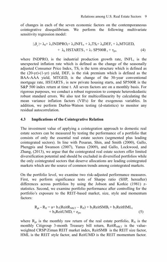
Relations among U.S. Real Estate Sectors 9
of changes in each of the seven economic factors on the contemporaneous
cointegrative disequilibrium. We perform the following multivariate
sensitivity regression model:
| |= λ0+ λ1INDPROt+ λ2INFLt + λ3TSt+ λ4DEFt + λ5MTGEDt
+ λ6 HSTARTS t + λ7 SP500R t + τpt, (4)
where INDPROt is the industrial production growth rate, INFLt is the
unexpected inflation rate which is defined as the change of the seasonally
adjusted Consumer Price Index, TSt is the term structure which is defined as
the (20-yr)-(1-yr) yield, DEFt is the risk premium which is defined as the
BAA-AAA yield, MTGEDt is the change of the 30-year conventional
mortgage rate, HSTARTS t is new private housing starts, and SP500R is the
S&P 500 index return at time t. All seven factors are on a monthly basis. For
rigorous purposes, we conduct a robust regression to compute heteroskedastic
robust standard errors. We also test for multicollinearity by calculating the
mean variance inflation factors (VIFs) for the exogenous variables. In
addition, we perform Durbin-Watson testing (d-statistics) to monitor any
residual autocorrelation.
4.3 Implications of the Cointegrative Relation
The investment value of applying a cointegration approach to domestic real
estate sectors can be measured by testing the performance of a portfolio that
consists of only the essential real estate sectors (segmented plus leading
cointegrated sectors). In line with Pesaran, Shin, and Smith (2000), Gallo,
Phengpis and Swanson (2007), Yunus (2009), and Gallo, Lockwood, and
Zhang, (2013), we argue that the cointegrated real estate sectors offer limited
diversification potential and should be excluded in diversified portfolios while
the only cointegrated sectors that deserve allocations are leading cointegrated
markets which are the source of common trends among cointegrated markets.
On the portfolio level, we examine two risk-adjusted performance measures.
First, we perform significance tests of Sharpe ratio (SHP, hereafter)
differences across portfolios by using the Jobson and Korkie (1981) z-
statistics. Second, we examine portfolio performance after controlling for the
portfolio’s exposure to the REIT-based market, size, style and momentum
factors:
Rpt - Rft = a+ b1(ReitRMKT – Rft) + b2ReitSMBt + b3ReitHMLt
+ b4ReitUMDt + ept, (5)
where Rpt is the monthly raw return of the real estate portfolio, Rft is the
monthly Citigroup 3-month Treasury bill return, ReitRMKT is the value-
weighted CRSP/Ziman REIT market index, ReitSMB is the REIT size factor,
HML is the REIT style factor, and ReitUMD is the REIT momentum factor.
t

10 Gallimore et al.
We test the performance of each portfolio by examining the sign and
significance of the estimate of the intercept. The intercept measures the
incremental performance (abnormal return) of the portfolio after controlling
for exposure to the broad market, size, style, and momentum factors. A
significant positive (negative) t-statistic for the intercept estimate indicates
superior (inferior) risk-adjusted performance.
Next, we hypothesize that cointegrated real estate sector indices become more
cointegrated in down markets so that cointegrated redundant sectors lack any
diversification benefit during down markets while essential ones should
outperform. We therefore conduct a performance test by running Equation (5)
over varying market conditions based on the performance of the benchmark
MKT. As defined above, an up market is the months in which the excess MKT
return is positive. A down market is defined as the months in which the excess
MKT return is non-positive. Between 01/1995 and 12/2009, our sample is
demarcated with 108 months of up markets and 72 months of down markets.
The first portfolio formation in 01/1995 is based on cointegration tests over
the 03/1984 to 12/1994 window. The portfolio is then held for 12 months and
rebalanced every January thereafter.11
Finally, similar to Chaudhry, Myer, and Webb (1999) and Yunus, Hansz, and
Kennedy (2012), we present the model specification for price discovery and
cointegration forecasting purposes based on the entire sample period from
1984 to 2009.
5. Empirical Results
Descriptive statistics are calculated over a 310-month sample period, March
1984 to December 2009, for each REIT sector index and are reported in Table
1. Other than the means, standard deviations, market capitalizations, and SHP,
we also report the Jobson-Korkie statistics for equality of the SHP of the REIT
sector versus that of the MKT.
The mean monthly return of the MKT equaled 0.82% with a 0.09 SHP over
the full sample period. The mean returns of the REIT sectors exhibit
substantial variation, ranging from a low of 0.25% for LODG to a high of
1.33% for HEAL. The Jobson-Korkie statistics indicate that only the SHP of
HEAL is significantly larger than that of the MKT (z-stat=2.24). The SHP of
the other sector indices are either smaller than or indifferent from that of the
MKT. The mean market capitalization shows that INDU had the highest
market value with a 27.39% market share among all other REIT sectors while
11 For example, the second portfolio formation in 01/1996 is based on cointegration
tests over the 01/1986 to 12/1995 window and the third portfolio formation in 01/1997
is based on cointegration tests over the 01/1987 to 12/1996 window, and so on and so
forth.

Relations among U.S. Real Estate Sectors 11
Table 1 Descriptive Statistics
INDEX RET(%) SD (%) SHP J-K z-stat
(vs. MKT) Mkt. Cap. Mkt. Share Count ConRatio R-Sqr P-value
Market Index 0.82% 4.95% 0.09 $124,000 100% 170.19 17.31%
3MTB 0.38% 0.19%
REIT Type
Unclassified (UNCL) 0.54% 5.21% 0.03 -1.36 $5,790 5.41% 18.17 73.71% 0.52 0.00***
Health Care (HEAL) 1.33% 5.56% 0.17 2.24** $8,480 7.93% 10.88 70.21% 0.63 0.00***
Industrial/Office (INDU) 0.57% 6.30% 0.03 -2.16** $29,300 27.39% 29.43 53.72% 0.79 0.00***
Lodging/Resorts (LODG) 0.25% 9.10% -0.01 -2.41** $9,214 8.61% 10.01 85.69% 0.52 0.00***
Residential (RESI) 0.97% 5.23% 0.11 0.84 $19,900 18.60% 22.16 58.79% 0.77 0.00***
Retail (RETL) 1.04% 5.79% 0.11 1.31 $28,700 26.83% 31.19 51.11% 0.88 0.00***
Self Storage (SELF) 1.11% 6.00% 0.12 0.76 $5,577 5.21% 7.26 88.04% 0.50 0.00***
Notes: This exhibit summarizes the monthly performance of the value-weighted REIT indices examined over a 310-month period,03/1984-
12/2009. Market Index is the CRSP/Ziman value-weight market index. 3MTB is the 3-month Treasury bill. For each index, we report the
raw mean return (RET), standard deviation of returns (SD), Sharpe ratio (SHP), and Jobson-Korkie statistic (J-K z-stat) for the equality of
the SHP with the SHP of the MKT. Mkt. Cap. represents the average market value of each REIT in millions. Count represents the average
number of REITs eligible for inclusion in the index. ConRatio is the concentration ratio that is the ratio of the market value of the largest
four securities in the portfolio versus the market value of the entire portfolio computed by using the beginning of period market caps. To
examine by how much the market return can be explained by a certain real estate type return, we adopt a single factor model as follows:
RtMKT= AlphaP + BetaP*RtP+ Errp
where RtMKT represents the REIT market raw return and RtPis the raw return of the real estate type index P. R-Sqr shows the goodness of
fit of the single factor model. P-value is for the F-test of model fitness. ***and ** and * denote statistical significance at the 1%, 5%, and
10% levels, respectively.
Relatio
ns am
ong
U.S
. Real E
state Secto
rs 11

12 Gallimore et al.
SELF with a 5.21% market share is ranked the lowest. The count ranged from
7.26 (SELF) to 31.19 (RETL), and on average, there was about 170 REITs
included in the market index over the sample period. The ConRatio indicates
that the market value of the largest four REITs occupied 88.04% (highest) of
the SELF portfolio while it was 51.11% (lowest) for the RETL portfolio. In
the spirit of Glascock and Kelly (2007), we run the MKT returns against each
real estate sector return to see by how much the MKT can be separately
explained by each sector. We find large R-squares under each real estate sector
regression with significant model F-test statistics which mean that real estate
sectors explain a large portion of the return variation in the domestic real
estate MKT. These findings are different from those of Glascock and Kelly
(2007), in which there is a 6% explanatory power of the sectors in the
international real estate markets. We conclude that real estate sectors provide
important diversification within the U.S. REIT market. The time series plot of
the log of price for these seven real estate sectors is presented in Figure 1.
Figure 1 Log of Price for Seven Real Estate Type REITs
(03/1984-12/2009)
Notes: Test period is from 03/1984 to 12/2009 which includes 310 monthly
observations. Figure 1 plots the log of price for seven real estate type REITs:
LPUNCL is the log price of unclassified REIT index; LPHEAL is the log
price of healthcare REIT index; LPINDU is the log price of industrial/office
REIT index; LPLODG is the log price of lodging/resort REIT index; LPRESI
is the log price of residential REIT index; LPRETL is the log price of retail
REIT index; and LPSELF is the log price of self-storage REIT index.
The cointegration methodology begins with unit root tests on the seven sector
price indices. We conduct five unit root tests, ADF, PP, KPSS, ZA, and NP, to
test the stationarity of each sectoral price index. Except for the KPSS test, all
the other unit root tests examine the null hypothesis of a unit root and non-
stationary against the alternative hypothesis that no unit root is present and the
data series is stationary. As shown in Table 2, we find that each of these seven
sector price indices has a unit root representation which is a non-stationary

Relations among U.S. Real Estate Sectors 13
I(1) process. No structure break is detected by the ZA test on the price level.
Therefore, unit root tests merit the implementation of the cointegration
methodology to further detect long-term equilibrium among non-stationary
sectoral price indices.
Table 2 Unit Root Tests from 03/1984 to 12/2009
Sector Index ADF PP KPSS (mu) ZA (Break) )(aMZ )(b
tMZ
UNCL -2.04 -1.00 4.35*** -3.92 (2000:08) -0.03 -0.02
HEAL -1.38 -1.35 5.90*** -4.14 (1998:04) 1.27 2.14
INDU -1.60 -0.76 4.41*** -3.88 (1990:07) -1.55 -0.68
LODG -7.42 -1.89 0.79*** -4.62 (1989:10) -7.35 -1.89
RESI -1.01 -0.53 6.17*** -3.70 (2006:01) 1.11 1.44
RETL -2.13 -1.22 5.90*** -3.16 (2004:05) 0.79 0.92
SELF -0.04 -0.02 6.03*** -3.54 (1989:10) 1.41 1.82
Note: Test period is the 310-month period from 03/1984 to 12/2009. Five unit root
tests are performed on the price levels of each data series: augmented Dicky-
Fuller (ADF), Phillips-Perron (PP), Kwiatkowski, Phillips, Schmidt, Shin
(KPSS), Zivot-Andrews (ZA) and Ng-Perron (NG). ADF, PP, ZA, NG tests all
examine the null hypothesis of a unit root and nonstationary against the
alternative hypothesis that no unit root is present and the data series is
stationary. The KPSS tests the null hypothesis of no unit root present and the
data is stationary. All tests allow for a maximum of 12 lags. The ZA test uses
AIC criteria to decide the lag length from a maximum of 12 lags. ADF joint test
of unit root critical values: 1%= 6.47, 5%= 4.61, and 10%= 3.79; PP unit root
test critical values: 1%= -3.468, 5%= -2.878, and 10%= -2.575 (reported
statistics are with 4 lags); ZA unit root test (Model C which allows break=both,
maximum 12 lags) critical values: 1%= -5.57, 5%= -5.08, and 10%= -4.82;
KPSS unit root test with mu statistics (H0: stationary around a level) critical
value: 1%= 0.739 and 5%= 0.463 and 10%=0.347 (reported statistics are with 4
lags). Ng and Perron (2001) MZa statistic critical value: 1%= -23.80, 5%= -
17.30, and 10%= -14.20. Ng and Perron (2001) MZt statistic critical value: 1%=
-3.42, 5%= -2.91, and 10%= -2.62. ***, **, and * denote statistical significance
at the 1%, 5%, and 10% levels, respectively.
The results of the cointegration tests are presented in Table 3. To ensure that
our cointegration tests are not look-ahead biased and suitable for an out-of-
sample portfolio formation, we follow Phengpis and Swanson (2010) and run
cointegration tests by using a 120-month rolling window approach with the
first window that ranges from 03/1984 to 12/1994 which instructs us to form
the COI portfolios on 01/1995 and hold them for the next 12 months. The
second window is from 01/1986 to 12/1995 for the 01/1996 formation, and so
on and so forth until the last window is from 01/1999 to 12/2008 for the
01/2009 formation. From the cointegration tests for fifteen separate rolling
windows, we reach consistent results in terms of cointegrated/segmented and
leading/following sectors. This finding is in line with the essence of the
cointegration framework, that in general, a long-term stable cointegrative

14 Gallimore et al.
relation is warranted should the cointegrating ECM hold. Furthermore, we
present a recursive cointegration test of CIV stability to show that the
cointegration test results are stable over time from 1995-2009. To conserve
space, we only report the results from the cointegration tests for the first
window. Other subsequent windows and the full period results are available
from the authors upon request.
Although the price series for all seven REIT sectors are with unit root
representation over the entire sample period as reported in Table 2, it is
necessary to further confirm if they are an I(1) process under each sub-period
in which we conduct the cointegration tests. Table 3A first reports chi-square
testing with stationary as the null hypothesis given the cointegration space.
We confirm that all sector price indices are non-stationary. Table 3B shows a
significant CIV among the seven real estate sector indices (Bartlett
λtrace=152.22, p-value=0.04) with insignificant G(r) common linear trend
components (p-value=0.17). The results from the cointegration exclusion tests
are reported in Table 3C. Sector indices with significant (insignificant) L-R
test statistics are cointegrated (segmented). The findings indicate that five
sectors: HEAL (L-RHEAL=5.81), INDU (L-RINDU=7.15), LODG (L-
RLODG=5.49), RETL (L-RRETL=3.62) and SELF (L-RSELF=4.27), are
cointegrated and share one CIV.12
However, the L-R statistics are insignificant
for UNCL (L-RUNCL=0.55) and RESI (L-RRESI=0.39), which imply their
segmentation from the cointegrative space. The robustness test, presented in
Table 3D, confirms there is one and only one significant CIV among all five
cointegrated real estate sectors (Bartlett λtrace=72.07, p-value=0.03) with a
similar insignificant G(r) common linear trend component (p-value=0.28).
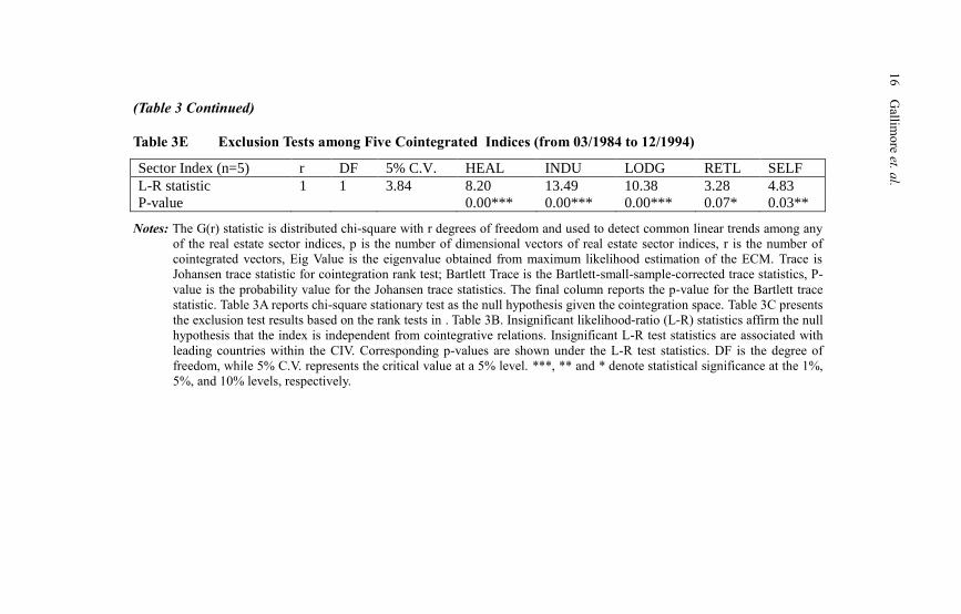
Table 3E further confirms that none of the cointegrated REITs are segmented
from the cointegrative space. Chaudhry, Myer, and Webb (1999) find one
cointegative relation among four real estate sectors and there is a positive
long-term cointegrative relation between retail and office. Our results support
the findings of Chaudhry, Myer, and Webb (1999). From the Johansen
cointegration rank and exclusion tests, we conclude that HEAL, INDU,
LODG, RETL, and SELF are cointegrated while UNCL and RESI areoutside
the cointegrating space.
12 The residual of our ECM model is stationary with 1 lag. The length of our lag is
determined by Ljung-Box statistics. Insignificant Ljung-Box statistics imply no
autocorrelation once 1 lag is imposed in the model. Although not reported, the test
result with 2 lags consistently finds 1 cointegrating vector. Since the use of more lags
sacrifices the degree of freedom, we keep the most parsimonious model with 1 lag.

Relations among U.S. Real Estate Sectors 15
Table 3A Stationarity Tests on all Indices (from 03/1984 to 12/1994)
UNCL HEAL INDU LODG RESI RETL SELF
L-R statistic 31.13 36.20 44.54 36.40 38.60 39.76 38.38
P-value 0.00*** 0.00*** 0.00*** 0.00*** 0.00*** 0.00*** 0.00***
Table 3B Cointegration Rank Tests on all Indices (from 03/1984 to 12/1994)
I(1)-Analysis
(n=7, lag=1) G(r) p-r r Eig. Value Trace Bartlett Trace P-Value Bartlett P-Value
1.90 7 0 0.29 156.63 152.22 0.02** 0.04**
P-value=0.17 6 1 0.25 111.63 108.99 0.11 0.16
Table 3C Exclusion Tests among all Indices (from 03/1984 to 12/1994)
Sector Index (n=7) r DF 5% C.V. UNCL HEAL INDU LODG RESI RETL SELF
L-R statistic 1 1 3.84 0.35 5.81 7.15 5.49 0.76 3.62 4.27
P-value 0.55 0.02** 0.01** 0.02** 0.39 0.06* 0.04*
Table 3D Cointegration Rank Tests on Five Cointegrated Indices (from 03/1984 to 12/1994)
I(1)-Analysis
(n=5, lag=1) G(r) p-r r Eig. Value Trace Bartlett Trace P-Value Bartlett P-Value
1.15 5 0 0.26 73.49 72.07 0.02** 0.03**
P-value=0.28 4 1 0.11 34/86 34.34 0.46 0.49
(Continued…)
R
elation
s amo
ng
U.S
. Real E
state Secto
rs 15
16 Gallimore et al.
(Table 3 Continued)
Table 3E Exclusion Tests among Five Cointegrated Indices (from 03/1984 to 12/1994)
Sector Index (n=5) r DF 5% C.V. HEAL INDU LODG RETL SELF
L-R statistic 1 1 3.84 8.20 13.49 10.38 3.28 4.83
P-value 0.00*** 0.00*** 0.00*** 0.07* 0.03**
Notes: The G(r) statistic is distributed chi-square with r degrees of freedom and used to detect common linear trends among any
of the real estate sector indices, p is the number of dimensional vectors of real estate sector indices, r is the number of
cointegrated vectors, Eig Value is the eigenvalue obtained from maximum likelihood estimation of the ECM. Trace is
Johansen trace statistic for cointegration rank test; Bartlett Trace is the Bartlett-small-sample-corrected trace statistics, P-
value is the probability value for the Johansen trace statistics. The final column reports the p-value for the Bartlett trace
statistic. Table 3A reports chi-square stationary test as the null hypothesis given the cointegration space. Table 3C presents
the exclusion test results based on the rank tests in . Table 3B. Insignificant likelihood-ratio (L-R) statistics affirm the null
hypothesis that the index is independent from cointegrative relations. Insignificant L-R test statistics are associated with
leading countries within the CIV. Corresponding p-values are shown under the L-R test statistics. DF is the degree of
freedom, while 5% C.V. represents the critical value at a 5% level. ***, ** and * denote statistical significance at the 1%,
5%, and 10% levels, respectively.
1
6 G
allimo
re et. al.
Relations among U.S. Real Estate Sectors 17
We contend that cointegrated real estate sectors share common underlying
trends and thus co-move temporally, which undermines diversification
benefits. However, leading indices within a CIV do not respond to deviations
from the cointegrative relation, and although cointegrated, may still offer
diversification benefits (Pesaran, Shin, and Smith 2000, Yunus 2009, Gallo,
Lockwood, and Zhang 2013). To differentiate leading sectors from
subordinate following sectors, we conduct a Granger (1969) causality test.
The Granger-causality test is to identify if one variable improves the
forecasting performance of another variable. If the price indices are
cointegrated, as suggested by Engle and Granger (1987), an error correction
term needs to be imposed in the Granger-causality relation as follows:
T1,..., t,...11 ttktktt XXX (6)
where tX is a )15( matrix of the returns of the five cointegrated sectors,
is a )15( vector of the constants, iΓ is a )55( matrix of the beta
coefficients, itX is a )15( matrix of the lagged endogenous return
variables, and t is a )15( matrix of the white noise error terms. t isthe
error correction term that measures the response to deviations from the
cointegrative equilibrium among the five cointegrated sectors. As mentioned
in Granger (1988), the causation of the endogenous variable by the exogenous
variables within the ECM can be either through the lagged values of the
exogenous variables or the error correction term, t . To test if one sector
Granger-causes the other in the short-term, we test if the coefficient on the
lagged endogenous sector returns are jointly significant as measured by the F-
statistic or if the coefficient of the t is significant as measured by the T-
statistic.
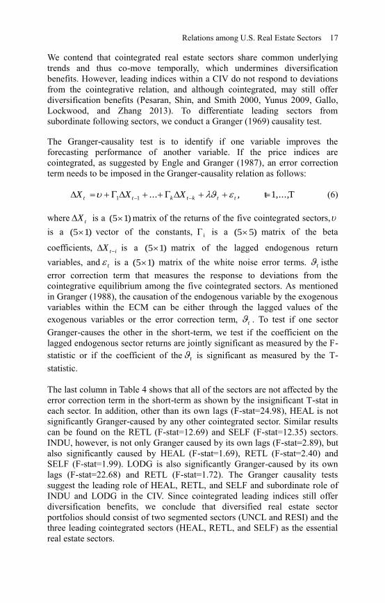
The last column in Table 4 shows that all of the sectors are not affected by the
error correction term in the short-term as shown by the insignificant T-stat in
each sector. In addition, other than its own lags (F-stat=24.98), HEAL is not
significantly Granger-caused by any other cointegrated sector. Similar results
can be found on the RETL (F-stat=12.69) and SELF (F-stat=12.35) sectors.
INDU, however, is not only Granger caused by its own lags (F-stat=2.89), but
also significantly caused by HEAL (F-stat=1.69), RETL (F-stat=2.40) and
SELF (F-stat=1.99). LODG is also significantly Granger-caused by its own
lags (F-stat=22.68) and RETL (F-stat=1.72). The Granger causality tests
suggest the leading role of HEAL, RETL, and SELF and subordinate role of
INDU and LODG in the CIV. Since cointegrated leading indices still offer
diversification benefits, we conclude that diversified real estate sector
portfolios should consist of two segmented sectors (UNCL and RESI) and the
three leading cointegrated sectors (HEAL, RETL, and SELF) as the essential
real estate sectors.
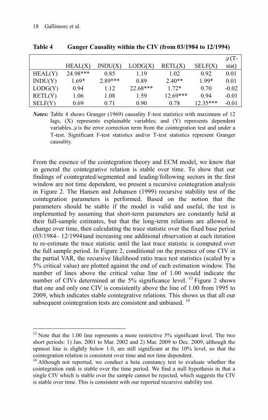
18 Gallimore et al.
Table 4 Ganger Causality within the CIV (from 03/1984 to 12/1994)
HEAL(X) INDU(X) LODG(X) RETL(X) SELF(X)
(T-
stat)
HEAL(Y) 24.98*** 0.85 1.19 1.02 0.92 0.01
INDU(Y) 1.69* 2.89*** 0.89 2.40** 1.99* 0.01
LODG(Y) 0.94 1.12 22.68*** 1.72* 0.70 -0.02
RETL(Y) 1.06 1.08 1.59 12.69*** 0.94 -0.01
SELF(Y) 0.69 0.71 0.90 0.78 12.35*** -0.01
Notes: Table 4 shows Granger (1969) causality F-test statistics with maximum of 12
lags, (X) represents explainable variables; and (Y) represents dependent
variables. is the error correction term from the cointegration test and under a
T-test. Significant F-test statistics and/or T-test statistics represent Granger
causality.
From the essence of the cointegration theory and ECM model, we know that
in general the cointegrative relation is stable over time. To show that our
findings of cointegrated/segmented and leading/following sectors in the first
window are not time dependent, we present a recursive cointegration analysis
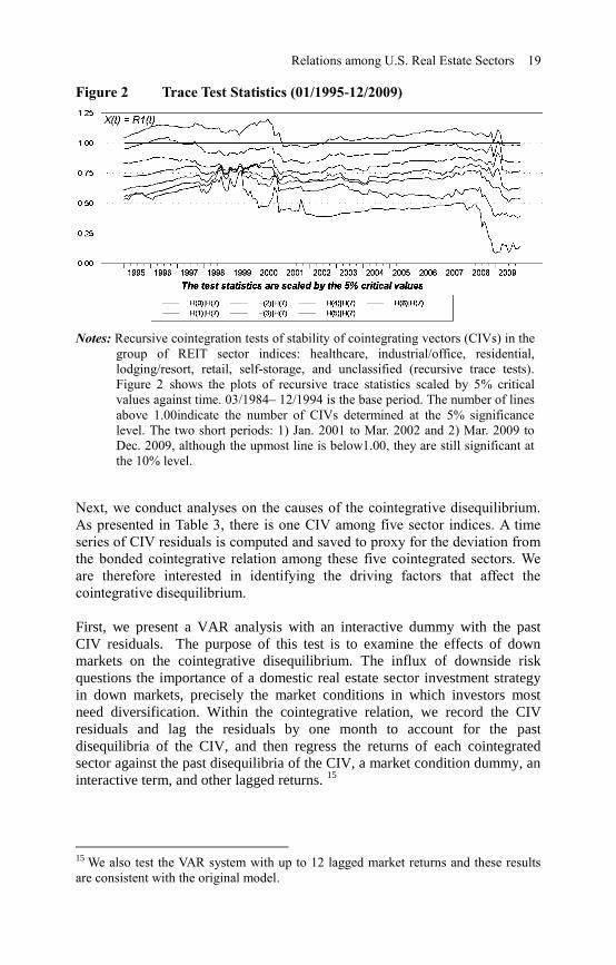
in Figure 2. The Hansen and Johansen (1999) recursive stability test of the
cointegration parameters is performed. Based on the notion that the
parameters should be stable if the model is valid and useful, the test is
implemented by assuming that short-term parameters are constantly held at
their full-sample estimates, but that the long-term relations are allowed to
change over time, then calculating the trace statistic over the fixed base period
(03/1984– 12/1994)and increasing one additional observation at each iteration
to re-estimate the trace statistic until the last trace statistic is computed over
the full sample period. In Figure 2, conditional on the presence of one CIV in
the partial VAR, the recursive likelihood ratio trace test statistics (scaled by a
5% critical value) are plotted against the end of each estimation window. The
number of lines above the critical value line of 1.00 would indicate the
number of CIVs determined at the 5% significance level. 13
Figure 2 shows
that one and only one CIV is consistently above the line of 1.00 from 1995 to
2009, which indicates stable cointegrative relations. This shows us that all our
subsequent cointegration tests are consistent and unbiased. 14
13 Note that the 1.00 line represents a more restrictive 5% significant level. The two
short periods: 1) Jan. 2001 to Mar. 2002 and 2) Mar. 2009 to Dec. 2009, although the
upmost line is slightly below 1.0, are still significant at the 10% level, so that the
cointegration relation is consistent over time and not time dependent. 14 Although not reported, we conduct a beta constancy test to evaluate whether the
cointegration rank is stable over the time period. We find a null hypothesis in that a
single CIV which is stable over the sample cannot be rejected, which suggests the CIV
is stable over time. This is consistent with our reported recursive stability test.
Relations among U.S. Real Estate Sectors 19
Figure 2 Trace Test Statistics (01/1995-12/2009)
Notes: Recursive cointegration tests of stability of cointegrating vectors (CIVs) in the
group of REIT sector indices: healthcare, industrial/office, residential,
lodging/resort, retail, self-storage, and unclassified (recursive trace tests).
Figure 2 shows the plots of recursive trace statistics scaled by 5% critical
values against time. 03/1984– 12/1994 is the base period. The number of lines
above 1.00indicate the number of CIVs determined at the 5% significance
level. The two short periods: 1) Jan. 2001 to Mar. 2002 and 2) Mar. 2009 to
Dec. 2009, although the upmost line is below1.00, they are still significant at
the 10% level.
Next, we conduct analyses on the causes of the cointegrative disequilibrium.
As presented in Table 3, there is one CIV among five sector indices. A time
series of CIV residuals is computed and saved to proxy for the deviation from
the bonded cointegrative relation among these five cointegrated sectors. We
are therefore interested in identifying the driving factors that affect the
cointegrative disequilibrium.
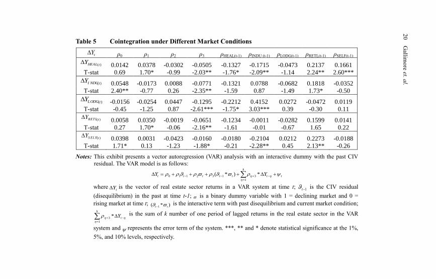
First, we present a VAR analysis with an interactive dummy with the past
CIV residuals. The purpose of this test is to examine the effects of down
markets on the cointegrative disequilibrium. The influx of downside risk
questions the importance of a domestic real estate sector investment strategy
in down markets, precisely the market conditions in which investors most
need diversification. Within the cointegrative relation, we record the CIV
residuals and lag the residuals by one month to account for the past
disequilibria of the CIV, and then regress the returns of each cointegrated
sector against the past disequilibria of the CIV, a market condition dummy, an
interactive term, and other lagged returns. 15
15 We also test the VAR system with up to 12 lagged market returns and these results
are consistent with the original model.
20 Gallimore et al.
Table 5 Cointegration under Different Market Conditions
tY ρ0 ρ1 ρ2 ρ3 ρHEAL(t-1) ρINDU (t-1) ρLODG(t-1) ρRETL(t-1) ρSELF(t-1)
0.0142 0.0378 -0.0302 -0.0505 -0.1327 -0.1715 -0.0473 0.2137 0.1661
T-stat 0.69 1.70* -0.99 -2.03** -1.76* -2.09** -1.14 2.24** 2.60***
0.0548 -0.0173 0.0088 -0.0771 -0.1321 0.0788 -0.0682 0.1818 -0.0352
T-stat 2.40** -0.77 0.26 -2.35** -1.59 0.87 -1.49 1.73* -0.50
-0.0156 -0.0254 0.0447 -0.1295 -0.2212 0.4152 0.0272 -0.0472 0.0119
T-stat -0.45 -1.25 0.87 -2.61*** -1.75* 3.03*** 0.39 -0.30 0.11
0.0058 0.0350 -0.0019 -0.0651 -0.1234 -0.0011 -0.0282 0.1599 0.0141
T-stat 0.27 1.70* -0.06 -2.16** -1.61 -0.01 -0.67 1.65 0.22
0.0398 0.0031 -0.0423 -0.0160 -0.0180 -0.2104 0.0212 0.2273 -0.0188
T-stat 1.71* 0.13 -1.23 -1.88* -0.21 -2.28** 0.45 2.13** -0.26
Notes: This exhibit presents a vector autoregression (VAR) analysis with an interactive dummy with the past CIV
residual. The VAR model is as follows:
t
k
tttttt YY
1
3132110 *)*(
wheretY is the vector of real estate sector returns in a VAR system at time t;
1t is the CIV residual
(disequilibrium) in the past at time t-1; is a binary dummy variable with 1 = declining market and 0 =
rising market at time t; )*( 1 tt is the interactive term with past disequilibrium and current market condition;
k
tY1
3 *
is the sum of k number of one period of lagged returns in the real estate sector in the VAR
system and represents the error term of the system. ***, ** and * denote statistical significance at the 1%,
5%, and 10% levels, respectively.
)(tHEALY
)(tI NDUY
)(tLODGY
)(tRETLY
)(tS ELFY
20
Gallim
ore et. a
l.

Relations among U.S. Real Estate Sectors 21
As presented in Table 5, two (three) out of five of the returns of the real estate
sectors significantly (insignificantly) and positively responded to their past
disequilibria in up markets, as indicated by the dummy variable ρ1. In
particular, in up markets, HEAL (ρ1=0.0378, t-stat HEAL,ρ1=1.70) and RETL
(ρ1=0.0350, t-statRETL,ρ1=1.70) deviated from their bonded long-term
equilibrium. However, all five cointegrated sectors significantly and
negatively reacted to their past disequilibria in down markets, captured by the
interactive term ρ1+ρ3. For instance, in down markets, HEAL moved towards
its long-term equilibrium by (ρ1+ρ3) =0.0378-0.0505=-0.0127 (t-statHEAL,ρ3=-
2.03). These findings suggest that cointegrated sectors become more
cointegrated in down markets as evidenced by movement towards their long-
term equilibrium. We report that the cointegrative relation among cointegrated
real estate sectors is in fact induced by down markets. This finding suggests
that cointegrated sectors lack diversification benefit during down markets
while essential ones should provide better downside risk protection. This
implies that we ought to look into different market conditions when
examining a cointegration-based portfolio strategy.
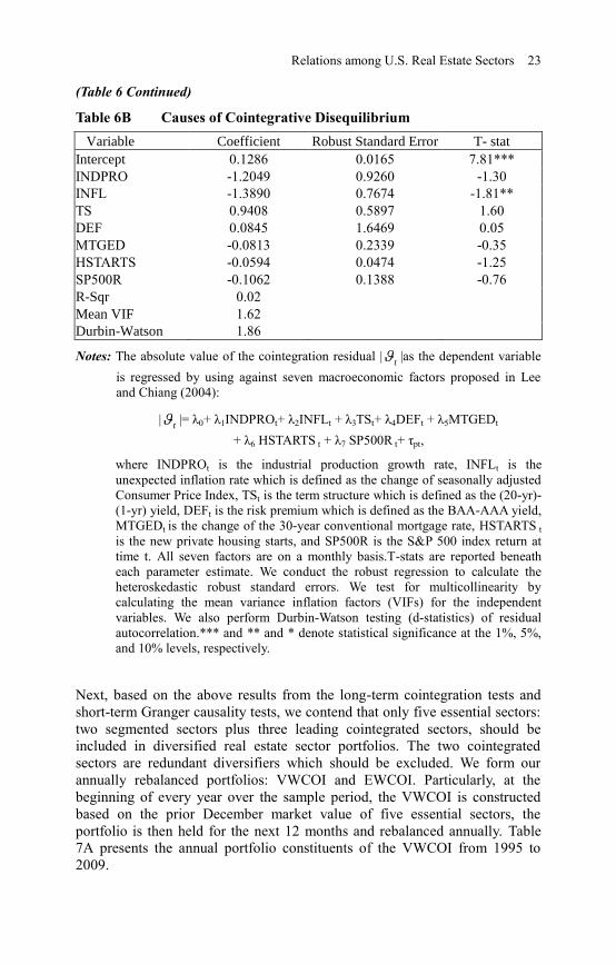
Second, we further examine the causes of the cointegrative disequilibrium by
running the absolute value of the CIV disequilibria against seven
contemporaneous economic factors proposed by Lee and Chiang (2004) who
find that industrial production affects both equity and mortgage REIT returns.
Besides that, Chan, Hendershott, and Sanders (1990) report that unexpected
inflation, changes in the risk premium, and term structures of interest rates
consistently drive equity REIT returns. Ling and Naranjo (1997) argue that
unexpected inflation and term structures of interest rates also systematically
affect real estate returns. Myer, Chaudry, and Webb (1997) also find that a
common factor, inflationary expectations, affects property values across
countries. Although we do not directly test the determinants of REIT returns,
the returns are closely related to the ECM residuals through the REIT prices.
Therefore, we expect that certain economic factors have impact on ECM
residuals as they affect real estate asset returns.
In Table 6A, we present the description, data source, and expected sign of
each of the seven exogenous variables in Equation 5. The data sources are
similar to those of Lee and Chiang (2004). Importantly, we list the anticipated
impacts of the exogenous variables on the absolute value of the cointegrative
disequilibrium. In particular, INDPRO is expected to have a positive sign
because a higher industrial production growth rate signals a better market
condition in general. According to our finding in Table 5 that real estate
sectors tend to be less cointegrated under up market conditions, we expect that
a higher industrial production growth rate will mean a larger deviation from
their bonded cointegrative relation. By the same token, a higher term structure
means a more upward sloping yield curve which signals a better market
condition so we anticipate a positive sign for the TS coefficient. Similarly,
higher new private housing starts mean better real estate market conditions, so
that a positive sign for the HSTARTS coefficient is expected as well. Ling and

22 Gallimore et al.
Naranjo (1999) and Okunev, Patrick and Zurbruegg (2000) find a strong
positive relation between U.S. stock and the real estate market, so we expect a
positive impact of the SP500R on the cointegrative disequilibrium.
On the contrary, we expect a negative sign for the INFL, DEF, and MTGED
coefficients. With respect to unexpected inflation, we anticipate a negative
sign in that high unexpected inflation translates into a pessimistic economic
state so that real estate sectors tend to cointegrate more under down market
conditions. High default risk premium also signals an unpleasant market
condition so we expect a negative sign as well. Similarly, high mortgage rate
means high borrowing costs to home buyers which lower real estate market
returns. A negative relation is anticipated between mortgage rate and the
cointegrative disequilibrium.
In Table 6B, we report the empirical results of Equation 5 and find that
unexpected inflation (λINFL=-1.3890, t-stat=-1.81) significantly and negatively
influences the absolute value of the cointegrative disequilibrium. When
experiencing higher unexpected inflation, a smaller disequilibrium error
indicates a greater cointegrating effect. The economic explanation for the
negative coefficient on the unexpected inflation is that with a high-unexpected
inflation shock, all of the domestic markets, including the real estate market,
would drop due to such unexpected unpleasant news that gives rise to lower
real estate market returns. Although the entire real estate market is declining,
different sectors might have a different declining pace due to the taste of the
investors.16
Therefore, the five cointegrated sectors become more cointegrated
under down real estate markets.
Table 6A Description of Exogenous Variables
Variable Description Data Source Expected Sign
INDPRO Industrial production
growth rate
Federal Reserve
Bank of St. Louis +
INFL Unexpected inflation rate Labor Bureaus of
Statistics -
TS Term structure Federal Reserve
Bank of St. Louis +
DEF Default risk premium Federal Reserve
Bank of St. Louis -
MTGED Change of 30-Year
mortgage rate
Federal Reserve
Bank of St. Louis -
HSTARTS New private housing
starts U.S. Census Bureau +
SP500R S&P 500 index return Center for Research
in Security Prices +
(Continued…)
16 We also conduct the same tests under sub-periods and varying market conditions,
and we find similar results. Unreported results are available upon request.
Relations among U.S. Real Estate Sectors 23
(Table 6 Continued)
Table 6B Causes of Cointegrative Disequilibrium
Variable Coefficient Robust Standard Error T- stat
Intercept 0.1286 0.0165 7.81***
INDPRO -1.2049 0.9260 -1.30
INFL -1.3890 0.7674 -1.81**
TS 0.9408 0.5897 1.60
DEF 0.0845 1.6469 0.05
MTGED -0.0813 0.2339 -0.35
HSTARTS -0.0594 0.0474 -1.25
SP500R -0.1062 0.1388 -0.76
R-Sqr 0.02
Mean VIF 1.62
Durbin-Watson 1.86
Notes: The absolute value of the cointegration residual | |as the dependent variable
is regressed by using against seven macroeconomic factors proposed in Lee
and Chiang (2004):
| |= λ0+ λ1INDPROt+ λ2INFLt + λ3TSt+ λ4DEFt + λ5MTGEDt
+ λ6 HSTARTS t + λ7 SP500R t+ τpt,
where INDPROt is the industrial production growth rate, INFLt is the
unexpected inflation rate which is defined as the change of seasonally adjusted
Consumer Price Index, TSt is the term structure which is defined as the (20-yr)-
(1-yr) yield, DEFt is the risk premium which is defined as the BAA-AAA yield,
MTGEDt is the change of the 30-year conventional mortgage rate, HSTARTS t
is the new private housing starts, and SP500R is the S&P 500 index return at
time t. All seven factors are on a monthly basis.T-stats are reported beneath
each parameter estimate. We conduct the robust regression to calculate the
heteroskedastic robust standard errors. We test for multicollinearity by
calculating the mean variance inflation factors (VIFs) for the independent
variables. We also perform Durbin-Watson testing (d-statistics) of residual
autocorrelation.*** and ** and * denote statistical significance at the 1%, 5%,
and 10% levels, respectively.
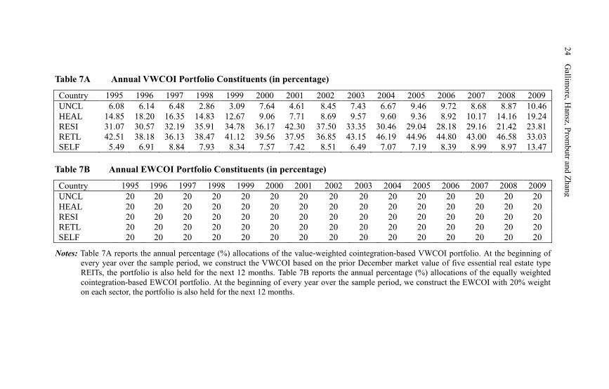
Next, based on the above results from the long-term cointegration tests and
short-term Granger causality tests, we contend that only five essential sectors:
two segmented sectors plus three leading cointegrated sectors, should be
included in diversified real estate sector portfolios. The two cointegrated
sectors are redundant diversifiers which should be excluded. We form our
annually rebalanced portfolios: VWCOI and EWCOI. Particularly, at the
beginning of every year over the sample period, the VWCOI is constructed
based on the prior December market value of five essential sectors, the
portfolio is then held for the next 12 months and rebalanced annually. Table
7A presents the annual portfolio constituents of the VWCOI from 1995 to
2009.
t
t
24 Gallimore et al.
Table 7A Annual VWCOI Portfolio Constituents (in percentage)
Country 1995 1996 1997 1998 1999 2000 2001 2002 2003 2004 2005 2006 2007 2008 2009
UNCL 6.08 6.14 6.48 2.86 3.09 7.64 4.61 8.45 7.43 6.67 9.46 9.72 8.68 8.87 10.46
HEAL 14.85 18.20 16.35 14.83 12.67 9.06 7.71 8.69 9.57 9.60 9.36 8.92 10.17 14.16 19.24
RESI 31.07 30.57 32.19 35.91 34.78 36.17 42.30 37.50 33.35 30.46 29.04 28.18 29.16 21.42 23.81
RETL 42.51 38.18 36.13 38.47 41.12 39.56 37.95 36.85 43.15 46.19 44.96 44.80 43.00 46.58 33.03
SELF 5.49 6.91 8.84 7.93 8.34 7.57 7.42 8.51 6.49 7.07 7.19 8.39 8.99 8.97 13.47
Table 7B Annual EWCOI Portfolio Constituents (in percentage)
Country 1995 1996 1997 1998 1999 2000 2001 2002 2003 2004 2005 2006 2007 2008 2009
UNCL 20 20 20 20 20 20 20 20 20 20 20 20 20 20 20
HEAL 20 20 20 20 20 20 20 20 20 20 20 20 20 20 20
RESI 20 20 20 20 20 20 20 20 20 20 20 20 20 20 20
RETL 20 20 20 20 20 20 20 20 20 20 20 20 20 20 20
SELF 20 20 20 20 20 20 20 20 20 20 20 20 20 20 20
Notes: Table 7A reports the annual percentage (%) allocations of the value-weighted cointegration-based VWCOI portfolio. At the beginning of
every year over the sample period, we construct the VWCOI based on the prior December market value of five essential real estate type
REITs, the portfolio is also held for the next 12 months. Table 7B reports the annual percentage (%) allocations of the equally weighted
cointegration-based EWCOI portfolio. At the beginning of every year over the sample period, we construct the EWCOI with 20% weight
on each sector, the portfolio is also held for the next 12 months.
24
Gallim
ore, H
ansz, P
rom
bu
tr and
Zh
ang

Relations among U.S. Real Estate Sectors 25
As presented in Table 7B, at the beginning of every year over the sample
period, the EWCOI is constructed based on 20% equal weight on each of the
five essential sectors, the portfolio is then held for the next 12 months. The
benefits of including leading sectors can be examined by comparing the
performance of the COI portfolios to portfolios that consist of only segmented
sectors (UNCL and RESI). Although not reported, we find that COI portfolios
outperformed the portfolios that contain only two segmented sectors which
support the inclusion of leading sectors into sufficiently diversified real estate
sector portfolios.
To understand the implications and investment value of the cointegrative
relation among real estate sectors, we compare the performance of our COI
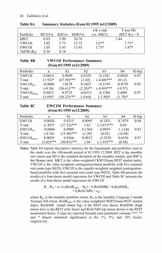
portfolios with the MKT portfolio over 01/1995 to 12/2009 in Table 8.17
Table
8A reports the average monthly return, standard deviation, SHP, Jobson-
Korkie statistics, and risk premium T-test statistics. The mean monthly return
for both the VWCOI (1.02% versus 0.93%, z-stat=1.67) and EWCOI(1.05%
versus 0.93%, z-stat=1.73) portfolios significantly exceeded the mean return
for the MKT. Annualized returns equaled 12.95% for the VWCOI portfolio,
13.35% for the EWCOI portfolio and 11.75% percent for the MKT
respectively. Both VWCOI and EWCOI risk premium were significantly
positive (t-statVWCOI=1.71; t-statEWCOI=1.87) while the MKT was less
attractive with an insignificant risk premium (t-statMKT=1.44). The Jobson-
Korkiez-stat indicates that the SHP is significantly higher for both the
VWCOI portfolio (12.72% vs. 10.78%) and EWCOI (13.95% vs. 10.78%)
versus the MKT, which is because the COI portfolios had a higher return
(RET) as well as lower risk (SD) than those of the MKT benchmark. In sum,
Table 8A indicates that domestic real estate investors would prefer the COI
portfolios over the all-sector MKT portfolio. These results confirm that the
inclusion of two non-leading cointegrated sectors (INDU and LODG) leads to
suboptimal asset allocations, thus resulting in inferior portfolio performance.
Tables 8B and 8C present the results of the four-factor model that control for
exposures to the broad REIT-based market, size, style, and momentum
factors. The results are consistent with the total risk findings reported in Table
8A. Importantly, both the VWCOI (aVWCOI=0.14%, t-stat=1.92) and EWCOI
(aEWCOI=0.20%, t-stat=1.85) portfolios exhibit superior significant abnormal
returns. Compounded annually, the abnormal returns equal 1.69% for the
VWCOI and 2.43% for the EWCOI portfolios, respectively. Not surprisingly,
17 Similar to the study by Ro and Ziobrowski (2011) which uses data from 1997 to
2006, this study examines the data from 1995 (the beginning of our portfolio
formation) to 2009. However, unlike Ro and Ziobrowski (2011) who use equity market
factors, MKTRP, SMB, HML and UMD, in their four-factor asset pricing model, we
use REIT-based market factors as suggested by recent studies by Hartzell, Mühlhofer
and Titman (2010) and Cici, Corgel and Gibson (2011).
26 Gallimore et al.
Table 8A Summary Statistics (from 01/1995 to12/2009)
Portfolio RET(%) SD(%) SHP(%)
J-K z-stat
(vs. MKT)
T-test H0:
(RET-Rf) = 0
MKT 0.93 5.90 10.78 1.44
VWCOI 1.02 5.75 12.72 1.67* 1.71*
EWCOI 1.05 5.45 13.95 1.73* 1.87*
3MTB (Rf) 0.38 0.19
Table 8B VWCOI Performance Summary
(from 01/1995 to12/2009)
Portfolio a b1 b2 b3 b4 R-Sqr
VWCOI 0.0014 0.9699 0.0329 -0.1581 0.0820 0.97
T-stat (1.92)* (67.59)*** (1.02) (-4.68)*** (0.13)
VWCOIUp -0.0006 1.0278 0.1025 -0.2159 -0.4759 0.93
T-stat (-0.36) (26.61)*** (2.24)** (-4.49)*** (-0.57)
VWCOIDown 0.0023 0.9733 -0.0313 -0.1204 2.4491 0.97
T-stat (1.69)* (56.32)*** (-0.64) (-1.90)* (1.78)*
Table 8C EWCIM Performance Summary
(from 01/1995 to12/2009)
Portfolio a b1 b2 b3 b4 R-Sqr
EWCOI 0.0020 0.9215 0.0995 -0.1831 0.7479 0.94
T-stat (1.85)* (37.32)*** 1.63 (-2.67)*** 0.69
EWCOIUp -0.0006 0.9090 0.1364 0.0919 -1.1144 0.83
T-stat (-0.34) (15.48)*** (1.20) (0.92) (-0.44)
EWCOIDown 0.0039 0.9266 0.0833 -0.2529 0.6356 0.97
T-stat (3.02)*** (30.83)*** 1.04 (-3.55)*** (0.56)
Notes: Table 8A reports descriptive statistics for the benchmark and portfolios used in
the study over the 180-month period of 01/1995-12/2009. RET is the monthly
raw return and SD is the standard deviation of the monthly returns, and SHP is
the Sharpe ratio. MKT is the value-weighted CRSP/Ziman REIT market index.
VWCOI is the value-weighted cointegration-based portfolio with five essential
real estate type REITs. EWCOI is the equally-weighted weighted cointegration-
based portfolio with five essential real estate type REITs. Table 8B presents the
results of a four-factor model regression for VWCOI and Table 8C presents the
results of a four-factor model regression for EWCOI:
Rt - Rft = a+ b1(ReitRMKT – Rft) + b2ReitSMBt + b3ReitHMLt
+ b4ReitUMDt + ept,
where Rpt is the monthly portfolio return, Rft is the monthly Citigroup 3-month
Treasury bill return, ReitRMKT is the value-weighted CRSP/Ziman REIT market
index, ReitSMB (small minus big) is the REIT size factor, ReitHML (high
minus low) is the REIT style factor and ReitUMD (up minus down) is the REIT
momentum factor. T-stats are reported beneath each parameter estimate.***, **
and * denote statistical significance at the 1%, 5%, and 10% levels,
respectively.

Relations among U.S. Real Estate Sectors 27
each of the two COI portfolios have a significant beta loading which shows
that REIT market premium significantly explains for the return variations of
the two portfolios. Notably, both cointegration-based portfolios VWCOI
(bVWCOI,1=0.9699) and EWCOI (bEWCOI,1=0.9215) have a beta smaller than
one, a proxy for a less systematic market risk than the all-sector MKT
portfolio. Both COI portfolios have an insignificant size loading
(bVWCOI,2=0.0329, t-stat=1.02; bEWCOI,2=0.0995, t-stat=-1.63) and momentum
loading (bVWCOI,4=0.0820, t-stat=0.13; bEWCOI,4=0.7479, t-stat=0.69) which
imply that COI portfolios consist of different sized REITs and both winner
and loser REITs of last year. Both COI portfolios also have a significant style
loading (bVWCOI,3=-0.1581, t-stat=-4.68; bEWCOI,3=-0.1831, t-stat=-2.67) which
implies that these portfolios tend to hold REITs with low Book-to-Market
ratios. In sum, any rational investor would prefer VWCOI and EWCOI over
the MKT.
From Table 5, we understand that cointegrated real estate sectors become
more cointegrated in down market conditions. Segmented real estate sectors
are expected to extend better performance (protection) for investors during
down markets. To further determine the extent to which general market
conditions impact on portfolio performance, we run performance tests
separated by up and down market conditions. The results are reported in Table
8B and 8C. Interestingly, no significant abnormal return is evident for both
COI portfolios during up markets which implies that these portfolios
performed indifferently from the MKT portfolio under good market
conditions. This finding also suggests that the overall outperformance of the
COI portfolios came from their superior performance under down markets.
Importantly, both the VWCOI and EWCOI portfolios significantly
outperformed the four-factor model during down markets (aVWCOI,Down=0.23%,
t-stat=1.69; aEWCOI,Down=0.39%, t-stat=3.02). Therefore, the COI portfolios
performed in line with the four-factor benchmark in up markets, but
significantly outperformed it by 23 basis points per month for the VWCOI
and 39 basis points for the EWCOI during down markets, thus effectively
providing a downside risk protection. Interestingly, we find that an equal-
weighted strategy, more easily implemented, provides better performance than
that of a more active value-weighted strategy. The results in Table 8 provide
an important finding that the better diversified cointegration-based portfolios,
VWCOI and EWCOI, which eliminated redundant diversifiers, provided
better protection to investors than an MKT during unfavorable market
conditions, in which investors most need diversification benefits.
Finally, similar to Chaudhry, Myer, and Webb (1999) and Yunus, Hansz, and
Kennedy (2012), we present the model specification for price discovery and
cointegration forecasting purposes based on the entire sample period from
1984 to 2009.

28 Gallimore et al.
Table 9A Cointegration Rank Tests (from 03/1984 to 12/2009)
I(1)-Analysis (n=5, lag=1) G(r) p-r r Eig.Value Trace Bartlett Trace P-Value Bartlett P-Value
1.50 5 0 0.13 65.73 65.21 0.00*** 0.00***
P-value=0.22 4 1 0.04 23.57 23.42 0.47 0.47
Table 9B Exclusion Tests (from 03/1984 to 12/2009)
REIT Index (n=5) r DF 5% C.V. HEAL INDU LODG RETL SELF
L-R statistic 1 1 3.84 12.39 28.16 11.89 22.67 8.11
P-value 0.00*** 0.00*** 0.00*** 0.00*** 0.00***
Table 9C BETA (transposed)
Log of Price HEAL INDU LODG RETL SELF
Beta(1) -4.954 -8.171 2.246 3.794 5.988
Beta(2) 4.383 0.475 0.903 -0.656 -3.38
Beta(3) -0.602 2.014 -2.991 -1.243 0.918
Beta(4) -4.734 -4.208 0.449 7.185 -0.03
Beta(5) 1.911 -1.588 0.804 -2.094 0.173
Notes: In Table 9A, the G(r) statistic is distributed chi-square with r degrees of freedom and used to detect common linear trends
among any of the real estate sector indices, p is the number of dimensional vectors of real estate sector indices, r is the
number of cointegrated vectors, Eig Value is the eigenvalue obtained from maximum likelihood estimation of the ECM.
Trace is Johansen trace statistic for cointegration rank test; Bartlett Trace is the Bartlett-small-sample-corrected trace
statistics, P-value is the probability value for Johansen trace statistics. The final column reports the p-value for the Bartlett
trace statistic. Table 9B presents the exclusion test results based on the rank tests in Table 9A. Insignificant likelihood-ratio
(L-R) statistics affirm the null hypothesis that the index is independent from cointegrating relations. Corresponding p-values
are shown under the L-R test statistics. DF is the degree of freedom, while 5% C.V. represents the critical value at a 5%
level. Table 9C reports the beta matrices which display the long-term relationship among the five cointegrated sectors in the
system. ***, ** and * denote statistical significance at the 1%, 5%, and 10% levels, respectively.
28
Gallim
ore et. a
l.

Relations among U.S. Real Estate Sectors 29
First, as expected, the results of the cointegration rank testing, as presented in
Table 9A, show that a significant CIV exists among the five aforementioned
cointegrated sectors(Bartlett λtrace=65.21, p-value=0.00) over the 1984-2009
period. Insignificant G(r) statistics (p-value=0.22) suggests that a linear trend
is not present in the cointegrative relation. Table 9B confirms that none of the
five cointegrated sectors are independent from their bonded long-term
cointegrative relation as suggested by significant L-R statistics. Table 9C lays
out the beta matrices that display the long-term relations among the five
cointegrated sectors in the system. Since one significant CIV is identified in
Table 9A, only the Beta (1) relationship is meaningful. Therefore, the long-
term cointegrative relation based on the full sample period (03/1984 to
12/2009) is as follows:
- 4.954HEALt - 8.171INDUt + 2.246LODGt + 3.794RETLt
+ 5.988SELFt = 0 (7)
where HEALt, INDUt, LODGt, RETLt, SELFt, are logs of price at time t. The
coefficient of each sector means the extent to which one sector reacts to other
sectors in the system. Equation (7) can be normalized with respect to any
variable in the model. For instance, the model can be rewritten as HEALt = -
1.649INDUt + 0.453LODGt + 0.766RETLt +1.209SELFt, so that in the long
run, a unit change in the INDU price index is expected to decrease the value
of the HEAL index by 1.649 while a unit change in the LODG, RETL, and
SELF price index is expected to increase the value of the HEAL index by
0.453, 0.766, and 1.209, respectively.18
Equation (7) discloses a price
discovery among the five cointegrated sectors for developing forecasts of real
estate prices.
6. Conclusion
This study extends the work of Chaudhry, Myer, and Webb (1999) by
investigating the long-term cointegrative relation among four real estate
sectors. Unlike Chaudhry, Myer, and Webb (1999), this study focuses on both
the long-term cointegrative and short-term causal relations among seven U.S.
real estate sector REITs from March 1984 to December 2009. Real estate
sector price indices are found to be non-stationary with unit root. By using
cointegration approaches, we find a significant cointegrative relation among
five real estate sectors (retail, industrial/office, lodging/resort, healthcare and
self storage) and the residential and unclassified sectors are segmented from
18 Chaudhry, Myer, and Webb (1999) report a positive long-term cointegrative relation
between retail and office. In particular, in the long run on a quarterly basis from 1978
to 1996, a unit change in the office price index increases the value of retail by 2.87
(retail = 2.87 office - 4.31 RD office + 1.45 ware). Our study is on a monthly basis
from 1984 to 2009 and we find that a unit change in the industrial/office price index
increases the value of retail by 2.154 (RETLt=1.306HEALt+2.154INDUt-
0.592LODGt-1.578SELFt).

30 Gallimore et al.
the cointegrative space. Among the five cointegrated sectors, the
industrial/office and lodging/resort sectors are found to be Granger-caused by
the retail, healthcare, and self-storage sectors so that these sectors are
considered as the leading indices while the industrial/office and lodging/resort
sectors are considered as the followers, which are redundant diversifiers. We
provide evidence that it is necessary to include leading cointegrated sectors
that sufficiently represent the cointegrating vector, but exclude redundant
cointegrated ones in diversified real estate sector portfolios.
Importantly, this study investigates the causes of cointegrative disequilibrium
among five cointegrated real estate sectors. Based on our proposed vector
autoregressive model, we find that cointegrated sectors have become more
cointegrated under down real estate markets. In addition, we conduct a
multivariate sensitivity regression model with seven macroeconomic
explanatory variables which show that unexpected inflation significantly and
negatively influences the cointegrative disequilibrium. These two proposed
models will help scholars to study the causes of disequilibrium of a
cointegrative relation and can be extended to international securitized markets
for future study.
Lastly, we provide evidence that cointegration-based portfolios have higher
raw returns as well as smaller standard deviations, as compared to a traditional
all-sector benchmark MKT portfolio. We argue that the inferior performance
of the MKT stems from two redundant cointegrated sectors: industrial/office
and lodging/resort. Moreover, by using a REIT-based four-factor asset-pricing
model with different market conditions, the cointergration-based strategy
provides good protection to investors under down markets, in which investors
most need diversification.
Since many REITs exclusively operate in the U.S. and institutional investment
portfolios often have specific U.S. real estate allocation mandates, our results
help to clarify real estate portfolio selection and allocation policy important to
institutional investors and real estate portfolio managers. The implications of
this study are limited to U.S. domiciled investors. It is of interest to consider
how these results hold for global real estate sector diversification, especially
when emerging real estate markets are considered. A better understanding of
the integration- convergence process of the real estate sector could be also
beneficial to academicians and practitioners. These proposed extensions
remain promising areas of future research.
Relations among U.S. Real Estate Sectors 31
Acknowledgement
We thank Xudong An, Katsiaryna Salavei Bardos, Paul Caster, Tsang
Desmond, Ahmed Ebrahim, Hendrik Devos, John G. Gallo, Xin James He,
Walter F. Hlawitschka, Gregory D. Koutmos, Larry Lockwood, Norman A.
Solomon, and Vishnu Vinekar for their comments. We thank three anonymous
reviewers and Ko Wang (the editor) for helpful comments. We also thank
seminar participants at the 2011 Annual Meeting of the American Real Estate
Society (ARES) conference in Seattle, Washington, the 2011 annual Financial
Management Association (FMA) Conference in Denver, Colorado, the 2012
Global Chinese Real Estate Congress (GCREC) Annual Conference in Macau,
China, and the fall 2012 research seminar at the Fairfield University. All
errors are our own.
References
Arshanapalli, B. and Doukas J. (1993). International stock market linkages:
Evidence from the pre- and post-October 1987 period, Journal of Banking &
Finance, 17, 193-208.
Bai, J. and Perron P. (2003). Computation and Analysis of Multiple Structural
Change Models. Journal of Applied Econometrics, 1, 1-22.
Carhart, M. (1997). On persistence of mutual fund performance. Journal of
Finance, 52, 57-82.
Chan, K.C., Hendershott P.H., and Sanders A.B. (1990). Risk and Return on
Real Estate: Evidence from Equity REITs. AREUEA Journal, 18, 431-452.
Chen, H., Downs D.H. and Patterson G.A. (2012). The Information Content of
REIT Short Interest: Investment Focus and Heterogeneous Beliefs, Real
Estate Economics, 40, 249-283.
Chaudhry, M.K., Christie-David R.A. and Sackley W.H. (1999). Long-term
Structural Price Relationships in Real Estate Markets. Journal of Real Estate
Research, 18, 335-354.
Chaudhry, M.K., Myer F.C. N. and Webb J.R. (1999). Stationarity and
cointegration in systems with real estate and financial assets. Journal of Real
Estate Finance and Economics, 18, 339-349.
Chiang, K.C.H. (2010). On the Comovement of REIT Prices, Journal of Real
Estate Research, 32, 187-200.

32 Gallimore et al.
Cici, G., Corgel J. B., and Gibson S. (2011). Can fund managers select
outperforming REITS? examining fund holdings and trades. Real Estate
Economics, 39, 455-486.
Dickey, D., and Fuller W. A. (1981). Likelihood Ratio Statistics for
Autoregressive Time Series with A Unit Root. Econometrica, 49, 1057-1072.
Eichholtz, P.M.A., Hoesli M., MacGregor B.D. and Nanthakumaran N.
(1995). Real estate portfolio diversification by property type and region.
Journal of Property Finance, 6, 39-59.
Engle, R.F. and Granger C.W.J. (1987). Co-Integration and Error Correction:
Representation, Estimation, and Testing. Econometrica, 55, 251-276.
Fabozzi, F. J., and Francis J. C. (1977). Stability tests for alphas and betas
over up and down market conditions. Journal of Finance, 32, 1093-1099.
Fama, E. F., and French K. R. (1993). Common Risk Factors in the Returns on
Stocks and Bonds. Journal of Financial Economics, 33, 3-56.
Gallo, J.G., and Zhang Y. (2010). Global Property Market Diversification,
Journal of Real Estate Finance and Economics, 41, 458-485.
Gallo, J.G., Lockwood L.J., and Zhang Y. (2013). Structuring Global Property
Portfolios: A Cointegration Approach, Journal of Real Estate Research,
forthcoming.
Gallo, J.G., Phengpis C. and Swanson P.E. (2007). Determinants of Equity
Style. Journal of Financial Services Research, 31, 33-51.
Glascock, J and Kelly L. (2007). The relative effect of property type and
country factors in reduction of risk of internationally diversified real estate
portfolios. Journal of Real Estate Finance and Economics, 34, 369-384.
Granger, C.W.J. (1969). Investigating causal relations by econometric models
and cross-spectral methods. Econometrica, 37, 424-438.
Granger, C.W.J. (1988). Some Recent developments in the concept of
causality, Journal of Econometrics, 39, 199-211.
Gyourko, J. and Nelling E. (1996). Systematic Risk and Diversification in the
Equity REIT Market, Real Estate Economics, 24, 493-515.
Hansen, H. and Johansen S. (1999). Some tests for parameter constancy in
cointegrated VAR-models. Econometrics Journal, 2, 306-333.
Relations among U.S. Real Estate Sectors 33
Hartzell, D., Hekman J. S., and Miles M. (1986). Diversification categories in
investment real estate. Journal of the American Real Estate and Urban
Economics Association, 14, 230-254.
Hartzell, J., Mühlhofer T., and Titman S. (2010). Alternative benchmarks for
evaluating REIT mutual fund performance. Real Estate Economics, 38,121-
154.
Hoesli, M. and Reka K. (2011). Volatility Spillovers, Comovements and
Contagion in Securitized Real Estate Markets, Journal of Real Estate Finance
and Economics, forthcoming.
Jobson, J.D., and Korkie B. (1981). Performance Hypothesis Testing with the
Sharpe and Treynor Measures. Journal of Finance,36, 889-908.
Johansen, S. (1988). Statistical Analysis of Cointegrating Vectors. Journal of
Economic Dynamics and Control, 12, 231-254.
Johansen, S. (1991). Estimation and Hypothesis Testing of Cointegrating
Vectors in Gaussian Vector Autoregressive Models. Econometrica, 59, 1551-
1580.
Johansen, S. (1992a). Determination of Cointegration Rank in the Presence of
a Linear Trend. Oxford Bulletin of Economics and Statistics, 54, 383-397.
Johansen, S. (1992b). Testing Weak Exogeneity and the Order of
Cointegration in UK Money Demand Data. Journal of Policy Modeling, 14,
313-334.
Johansen, S.(2002). A small sample correction for the test of cointegrating
rank in the vector autoregressive model. Econometrica, 71, 1929-1961.
Johansen, S., Mosconi R., and Nielsen B. (2000). Cointegration Analysis in
the Presence of Structural Breaks in the Deterministic Trend. The
Econometrics Journal, 3, 216-249.
Kim, K. (2003). Dollar exchange rate and stock price: evidence from
multivariate cointegration and error correction model. Review of Financial
Economics, 12, 301-313.
Kleiman, R.T., Payne J.E. and Sahu A.P. (2002). Random Walks and Market
Efficiency: Evidence from International Real Estate Markets. Journal of Real
Estate Research, 24, 279-298.
Kwiatkowski, D., Phillips P.C.B., Schmidt P., and Shin Y. (1992). Testing the
Null Hypothesis of Stationarity against the Alternative of a Unit Root. Journal
of Econometrics, 54, 159-178.
34 Gallimore et al.
Lee, S.L. (2001). The Relative Importance of Property Type and Regional
Factors in Real Estate Returns. Journal of Real Estate Portfolio Management,
7, 159-167.
Lee, S.L. and Byrne P. (1998). Diversification by sector, region or function? A
mean absolute deviation optimization .Journal of Property Valuation and
Investment, 16, 38-56.
Lee, M. L. and Chiang K. C. H. (2004). Substitutability between Equity
REITs and Mortgage REITs, Journal of Real Estate Research, 26, 95-114.
Ling, D.C. and Naranjo A. (1997). Economic Risk Factors and Commercial
Real Estate Returns. Journal of Real Estate Finance and Economics, 15, 283-
307.
Ling, D.C. and Naranjo A. (1999). The integration of commercial real estate
markets and stock markets. Real Estate Economics, 27, 483-515.
Ling, D.C., Naranjo A. and Ryngaert M. (2012). Real Estate Ownership,
Leasing Intensity, and Value: Do Stock Returns Reflect a Firm’s Real Estate
Holdings? Journal of Real Estate Finance and Economics, 2012, 44, 184-202.
Liow, K.H., Ho, K. H. D., Ibrahim, M. F. and Chen Z. (2009). Correlation and
Volatility Dynamics in International Real Estate Securities Markets, Journal
of Real Estate Finance and Economics, 39, 202-223.
Liu, X. and Zhang L. (2008). Momentum profits, factor pricing, and
macroeconomic risk. Review of Financial Studies, 21, 2417-2448.
Mananyi, A. and Struthers J.J. (1997). Cocoa market efficiency: a
cointegration approach, Journal of Economic Studies, 24, 141-151.
McCue, T.E. and Kling J.L. (1994). Real Estate Returns and the
Macroeconomy: Some Empirical Evidence from Real Estate Investment Trust
Data, 1972-1991. Journal of Real Estate Research, 9, 277-287.
Myer, F.C.N., Chaudhry M.K., and Webb J.R. (1997). Stationarity and Co-
integration in Systems with Three National Real Estate Indices. Journal of
Real Estate Research, 13, 369-381.
Narayana,P.K. and Smytha R. (2004). The relationship between the real
exchange rate and balance of payments: empirical evidence for China from
cointegration and causality testing, Applied Economics Letters, 11, 287-291.
Ng, S. and Perron P. (2001). Lag Length Selection and the Construction of
Unit Root Tests with Good Size and Power. Econometrica, 69,1519-1554.

Relations among U.S. Real Estate Sectors 35
Okunev, J., Patrick, W. and Zurbruegg R. (2000) The Causal Relationship
between Real Estate and Stock Markets, Journal of Real Estate Finance and
Economics, 21, 251-261.
Phengpis C. and Swanson P.E. (2010). Optimization, Cointegration and
Diversification Gains from International Portfolios: An Out of Sample
Analysis. Review of Quantitative Finance and Accounting, 36, 269-286.
Pesaran, M. H., Shin Y., and Smith R.J. (2000) Structural Analysis of Vector
Error Correction Models with Exogenous I(1) Variables. Journal of
Econometrics, 97, 293-343.
Peterson, J. D. and Hsieh C. (1997). Do Common Risk Factors in the Returns
on Stocks and Bonds Explain Returns on REITs? Real Estate Economics, 25,
321-345.
Phillips, P. C. B., and Perron P. (1988). Testing for a Unit Root in Time Series
Regression. Biometrika, 75, 335-346.
Richards, A.J. (1995). Comovements in national stock market returns:
Evidence of predictability, but not cointegration. Journal of Monetary
Economics, 36, 631-654.
Ro, S. and Ziobrowski A. (2011). Does focus really matter? Specialized vs.
Diversified REITs. Journal of Real Estate Finance and Economics, 42, 68-83.
Stevenson S. (2002). An Examination of Volatility Spillovers in REIT
Returns. Journal of Real Estate Portfolio Management, 8, 229-238.
Swaray, R. (2008). Macroeconomic Determinants of Non-Fuel Primary
Commodity Price Movements. Journal of Applied Business Research, 24, 11-
16.
Tarbert, H. (1998). The long-run diversification benefits available from
investing across geographical regions and property type: evidence from
cointegration tests. Economic Modeling, 15, 49-65.
Wilson, P. and Okunev J. (1996). Evidence of segmentation in domestic and
international property markets. Journal of Property Finance, 7, 78-97.
Wilson,P.J., Stevenson S. and Zurbruegg R.(2007). Foreign Property Shocks
and the Impact on Domestic Securitized Real Estate Markets: An Unobserved
Components Approach. Journal of Real Estate Finance and Economics, 34,
407-424.
36 Gallimore et al.
Wood, R.A. (1995). Cointegration, error correction, and price discovery on
informationally linked security markets. Journal of Financial and
Quantitative Analysis, 30, 563-579.
Young, M.S. (2000). REIT Property-Type Sector Integration. Journal of Real
Estate Research, 19, 3-21.
Yunus, N. (2009). Increasing Convergence between US and International
Securitized Property Markets: Evidence based on Cointegration Tests. Real
Estate Economics, 37, 383-411.
Yunus, N., Hansz J. A. and Kennedy P. J. (2012). Dynamic Interactions
between Private and Public Real Estate Markets: Some International
Evidence. Journal of Real Estate Finance and Economics, 45, 1021-1040.
Yunus, N. and Swanson P. E. (2007). Modeling linkages between U.S. and
Asia-Pacific securitized property markets. Journal of Property Research, 24:2,
95-122.
Yunus, N. and Swanson P. E. (2013). A closer look at the U.S. housing
market: Modeling relationships among regions. Real Estate Economics,
forthcoming.
Zivot, E., and Andrews D.W.K. (1992). Further Evidence on the Great Crash,
the Oil-Price Shock, and the Unit-Root Hypothesis. Journal of Business and
Economic Statistics, 10, 251-270.