Inverse Modeling of Tight Gas Reservoirs

Der Fakultät für Geowissenschaften, Geotechnik und Bergbau

der Technischen Universität Bergakademie Freiberg

eingereichte

Dissertation

Zur Erlangung des akademischen Grades

Doktor-Ingenieur

Dr.-Ing.

vorgelegt

von: Dipl.-Ing. Mtchedlishvili George

geboren am 01.10.1977 in Tbilisi, Georgien

Freiberg, den: 25.01.2007

2

Abstract

The present thesis focuses on the following issues: (i) inverse modeling techniques for characterization

of tight-gas reservoirs, (ii) the numerical investigations of advanced well stimulation techniques, such

as hydraulic fracturing as well as underbalanced drilling, and (iii) the statistical analyses of results for

identification of the optimal level of parameterization for calibrated model as quality and quantity of

the measured data justifies.

In terms of a considerable increase the quality of characterization of tight-gas reservoirs, the aim of

this work was (i) an accurate representation of technological aspects and specific conditions in a reser-

voir simulation model, induced after the hydraulic fracturing or as a result of the underbalanced drill-

ing procedure and (ii) performing the history match on a basis of real field data to calibrate the gener-

ated model by identifying the main model parameters and to investigate the different physical

mechanisms, e.g. multiphase flow phenomena, affecting the well production performance.

Due to the complexity of hydrocarbon reservoirs and the simplified nature of the numerical model, the

study of the inverse problems in the stochastic framework provides capabilities using diagnostic statis-

tics to quantify a quality of calibration and the inferential statistics that quantify reliability of parame-

ter estimates. As shown in the present thesis the statistical criteria for model selection may help the

modelers to determine an appropriate level of parameterization and one would like to have as good an

approximation of the structure of the system as the information permits.

3

Acknowledgment

First of all, I would like to thank my supervisor, Prof. Frieder Häfner, for his very kind encourage-

ment, support and guidance during this work.

I am very indebted to Dr. Aron Behr for very useful discussions and for the positive influence on my

professional career.

I wish to express my sincere thanks and gratitude to Dr. Hans-Dieter Voigt and Dr. Torsten Friedel,

who gave useful contributions at various times during the development of this thesis.

I am grateful to the staff of Institute of Drilling Engineering and Fluid Mining, TU Bergakademie

Freiberg.

Finally, my warmest thanks go to my family for their effort, moral support and love.

4

Content

ABSTRACT 2

ACKNOWLEDGMENT 3

CONTENT 4

NOMENCLATURA 7

LIST OF FIGURES 11

LIST OF TABLES 13

1 STATEMENT OF THE PROBLEM 14

2 AN INTRODUCTION TO INVERSE PROBLEMS 17

2.1 Reservoir Modeling 17

2.2 The Inverse Modeling 19 2.2.1 The Statistical Methods for Model Calibration 20

2.2.1.1 Statistical Criteria of Parameter Estimation with Homogeneous Prior Distribution 23 2.2.1.2 Statistical Criteria of Parameter Estimation with Gaussian Prior Distribution 24

2.3 Numerical Optimization Algorithms 25 2.3.1 Nonlinear Last Squares – Gradient Based Methods 27 2.3.2 Global-Optimization Techniques – Direct Search Methods 29

2.3.2.1 Neighbourhood Algorithm 29 2.3.3 Analyses of Parameter Estimation Uncertainties 33 2.3.4 Optimality and Model Identification Criteria 35

2.3.4.1 Kullback-Leibler Information 35 2.3.4.2 Alternative Model Selection Criteria 38

2.3.5 Application to the Synthetic Field Example 39 2.3.5.1 Reservoir Description and Parameterization 39 2.3.5.2 Simulation Results 40

5

3 SIMULATION OF THE PRODUCTION BEHAVIOR OF HYDRAULICALLY FRACTURED WELLS IN TIGHT GAS RESERVOIRS 46

3.1 Introduction to Fractured Well Simulation 47

3.2 Automatic Generaton of the Simulation Model for Fractured Wells 50 3.2.1 Local Grid Refinement 51 3.2.2 Integration of the Fracture Parameters 53 3.2.3 Estimation of the Fluid Distribution in the Invaded Zone 55

3.2.3.1 Evaluation of Exposure Time 55

3.3 History-Matching of a Case Study of Hydraulically Fractured Well 60 3.3.1 Field Example 60 3.3.2 Simulation Model 61 3.3.3 History Match 64

3.3.3.1 Cleanup with hydraulic damage 64 3.3.3.2 Combined effect of hydraulic and mechanical damage 67

3.3.4 Discussion of history match results 68 3.3.5 Effect of cleanup on postfracture performance 69

3.4 Identification of the Leakoff Coefficient by History Matching 71 3.4.1 Hypothetical Study 72 3.4.2 Case Study 76

3.5 Automatic Methods of Optimizing of Fractured Wells 79

4 SIMULATION OF INFLOW WHILEST UNDERBALANCED DRILLING (UBD)

WITH AUTOMATIC IDENTIFICATION OF FORMATION PARAMETERS AND ASSESSMENT OF UNCERTAINTY 84

4.1 Literature review 85

4.2 Simulation of Reservoir Flow during UBD 86

4.3 Parameter Estimation during UBD 87

4.4 Identification Procedure 88

4.5 Uncertainty Analyses 90

4.6 Example 91

4.7 Outlook: Optimization Approach for UBD 93

6

5 SUMMARY 94

BIBLIOGRAPHY 97

7

Nomenclatura

Symbols

Symbol Meaning Unit

A area,

sensitivity matrix

m²

a,b,c coefficients -

b set of subsidiary conditions

bf fracture width m

c proppant concentration kg/m²

Cl leakoff coefficient m/s1/2

Cl* specific leakoff coefficient m/s1/2 mDγ

Cov0 prior parameter-covariance matrix

Covz covariance matrix of measured values

d distance,

step size

m

F fractional flow, dimensionless -

FC fracture conductivity mD*m

FCD dimensionless fracture conductivity -

g Gradient vector

H Hessian matrix

J Jacobian matrix

I Unit matrix

k permeability,

index

m², Darcy

-

L linear size, m

M number of gridblocks

model

-

-

N number of pumping periods -

Nm number of measured data

Np number of model parameters

n coordinate normal to fracture plane m

ns,nr number of Voronoi cells

p pressure,

set of physical parameters

Pa

R number

8

r index

right-hand-side term

m³

q mass source/sink

set of control variables

kg/(m³*s)

-

S saturation -

s0 estimated error variance

t time sec

u set of state varaibles

V volume

x coordinate,

set of spatial and time variables

m

xf fracture half length m

Greek Symbols

Symbol Meaning Unit

α power factor,

fracture expansion factor

-

φ porosity -

∆, δ difference, increment -

ε error

γ power factor -

η net-to-gross thickness ratio -

µ dynamic viscosity Pa*s

µ0 viscosity ratio -

λ displacement direction,

regularization factor,

material parameter

-

Θ model parameter vector

ρ density kg/m³

σ effective stress,

standard deviation

MPa

ν velocity m/s

Ω domain

ω weight factor

ξ self-similar variable

9

Indices

Index Meaning

0 initial

a absolute

ad admissible

cap capillary

calc calculated

const constant

f fracture,

fictive

g gas

i index

phase index,

index of time period

j index

index of time period

k index

meas measured

obs observed

p proppant

pr primary

pred predictive

r relative

ref reference

s slurry

t total

w water

10

Functions and Operators

Function Meaning

AIC Akaike Information Criterion

BIC Bayesian Information Criterion

dm Kashyap Index

J Leverett J-Function

H statistical entropy

I information content

L partial differential operator,

likelihood

p probability density function

p0 prior distribution

p* posterior distribution

.∇ divergence operator

Abbreviations

Abbreviation Meaning

BHP Bottom Hole Pressure

CSS Composite Scaled Sensitivities

DF Discount rate

FOPT Field Oil Production Total

GOR Gas-Oil Ratio

GPR Gas Production Rate

LGR Local Grid Refinement

NPV Net Present Value

OF Objective Function

THP Tubing Head Pressure

TOL Tolerance Criteria

UBD Underbalanced Drilling

WGR Water Gas Ratio

11

List of Figures

FIGURE 1: RANDOM POINTS IN A 2D SPACE ....................................................................................................... 30 FIGURE 2 A UNIFORM RANDOM WALK RESTRICTED TO A CHOSEN VORONOI CELL ................................................ 31 FIGURE 3: TOP STRUCTURE MAP OF THE PUNQ CASE WITH WELL LOCATIONS (FROM FLORIS ET AL. ) .................. 44 FIGURE 4: TRUTH CASE: HORIZONTAL PERMEABILITY FIELDS FOR LAYERS 1, 3, 5............................................... 45 FIGURE 5: THE PRODUCTION DATA FOR THE WELL “PRO-4”............................................................................... 45 FIGURE 6: THE PREDICTION RESULTS ................................................................................................................ 45 FIGURE 7: PRIMARY REFINEMENT OF FRACTURE................................................................................................ 51 FIGURE 8: SECONDARY REFINEMENT OF WELL AND FRACTURE........................................................................... 52 FIGURE 9: (A) VARIATION OF THE FRACTURE WIDTH (FROM THE FRACTURE PACKAGE PROTOCOL). THE DASH LINE

SHOWS THE FICTIVE WIDTH (0.1 M) OF THE FRACTURE IN THE SIMULATION MODEL (B) DISTRIBUTION OF THE

PROPPANT CONCENTRATION AND FRACTURE CONDUCTIVITY BY THE ELLIPTICAL ZONES OVER THE FRACTURE

(CORRESPONDS TO THE FRACTURE PACKAGE PROTOCOL)........................................................................... 54 FIGURE 10: INTEGRATION OF THE FRACTURE INTO THE RESERVOIR MODEL (PERMEABILITY AND POROSITY

DISTRIBUTION) ....................................................................................................................................... 54 FIGURE 11: WATER DISTRIBUTION AROUND THE FRACTURE IN THE SIMULATION MODEL ...................................... 59 FIGURE 12: PRODUCTION HISTORY OF CASE-STUDY WELL.................................................................................. 61 FIGURE 13: PERMEABILITY DISTRIBUTION WITHIN FRACTURE PLANE ................................................................. 63 FIGURE 14: INITIAL WATER DISTRIBUTION AROUND THE FRACTURE AFTER THE LEAKOFF PROCESS. ...................... 63 FIGURE 15: PRODUCTION DATA AND HISTORY MATCH RESULTS OF CLEANUP PERIOD............................................ 66 FIGURE 16: HISTORY MATCH OF POSTPRODUCTION PERIOD ................................................................................ 66 FIGURE 17: FUNCTIONS OF RELATIVE PERMEABILITY GAS-WATER AND CAPILLARY PRESSURE .............................. 66 FIGURE 18: LONG TIME PRODUCTIVITY: COMPARISON OD PRODUCTIVITY OF UNDAMAGED WELL (IGNORING

CLEANUP) AND DAMAGED WELL WITH 500 BAR DRAWDOWN. .................................................................... 69 FIGURE 19: SIMULATED GAS PRODUCTION RATE AND CUMULATIVE WATER RECOVERY ........................................ 73 FIGURE 20: DEPENDENCE ON VARIOUS PARAMETERS ON THE COEFFICIENT (A) NORMALISED MAXIMUM GAS RATE

(B) NORMALISED GAS RATE SLOPE (C) NORMALISED GAS BREAKTHROUGH ................................................ 74 FIGURE 21: DEVELOPMENT OF WATER BACKFLOW FROM THE INVADED ZONE...................................................... 75 FIGURE 22: DEVELOPMENT OF GAS FLOW RATE AND WATER RECOVERY AT THE BOTTOM-HOLE DURING THE

CLEANUP PERIOD..................................................................................................................................... 77 FIGURE 23: PERMEABILITY CURVES MATCHED IN THE CASE STUDY AT FIXED γ =0 AND 0.5 ................................. 77

FIGURE 24: COMPARISON OF PRODUCTION DATA SIMULATED BY THE FIXED RELATIVE PERMABILITIES FOR

DIFFERENT γ -EXPONENTS....................................................................................................................... 78 FIGURE 25: NORMALIZED COSTS OF THE FRACTURE TREATMENT VERSUS FRACTURE CONDUCTIVITY AT THE FIXED

SLURRY VOLUME ..................................................................................................................................... 80 FIGURE 26: VARIATION THE ESTIMATED PARAMETERS DURING THE OPTIMIZATION PROCEDURE AND THE

DEVELOPMENT OF THE NET PRESENT VALUE.............................................................................................. 82 FIGURE 27: 3-D SURFACE OF THE OBJECTIVE FUNCTION .................................................................................... 82 FIGURE 28: OBJECTIVE FUNCTION CONTOUR GRAPHS ........................................................................................ 83

12

FIGURE 29: COMPONENTS FOR UBD ................................................................................................................ 85 FIGURE 30: WELLBORE GRID WITH SCHEMATIC OF BOUNDARY CONDITIONS DURING UBD .................................. 87 FIGURE 31: UBD COUPLING ............................................................................................................................ 90 FIGURE 32: MEASURED AND SIMULATED GAS RATES ........................................................................................ 91 FIGURE 33 ESTIMATED AND TRUE PERMEABILITY VERSUS DRILLED DEPTH ......................................................... 92 FIGURE 34: COMPOSITE SCALED SENSITIVITIES (CSS) ...................................................................................... 92 FIGURE 35: CONTROL AND OPTIMIZATION LOOP FOR UBD PROCESSES ............................................................... 93

13

List of Tables

TABLE 1: THE SET OF DIFFERENT PARAMETERIZED MODELS ............................................................................... 43 TABLE 2: RANKING THE MODELS WITH THE K-L DISTANCE ................................................................................ 43 TABLE 3: RANKING THE MODELS WITH DIFFERENT MODEL SELECTION CRITERIA................................................. 44 TABLE 4: RESERVOIR AND WELL PARAMETERS .................................................................................................. 60

14

1 STATEMENT OF THE PROBLEM

The economic viability of an oil/gas field development project is greatly influenced by the reservoir

production performance under the current and future operating conditions. In order to analyze the res-

ervoir performance and estimate reserves, engineers make use of numerical flow simulators that re-

quire a parameterization of reservoir properties, i.e. a reservoir model, as input. After the simulation

model is built and the forecast problem can be solved, i.e. we can forecast the response of the system

for different excitation, as a result, different management decisions can be compared and optimal deci-

sion can be selected based on certain criteria.

In practice, however, it is very difficult to construct an accurate simulation model for a geological

system. Assuming, that the governing mathematical equations of the constructed model satisfactorily

describe the original system the all physical parameters are difficult to measure accurately in the field.

Usually limited Information on the geological and geophysical background of the reservoir is available

from well tests, seismic surveys, logs etc. The main source of information from the system may come

in the form of production data, such as production rates and pressure behavior, all of them indirect

measurements of the physical parameters that describe the fluid flow through the reservoir. The goal is

to estimate reservoir parameters to be used as an input in the flow simulator in order to describe satis-

factorily the production performance.

Since the input-output relation of a correct simulation reservoir model must fit the observed excitation-

response relation of the original system, it is possible to indirectly estimate the reservoir model pa-

rameters by using these observation data. Model calibration, inverse modeling, history matching, pa-

rameter estimation are terms describing essentially the same technique of adjusting the model parame-

ters until a close match between simulated and measured data is obtained.

Automatic model calibration can be formulated as an optimization problem, which has to be solved in

the presence of uncertainty, because the available observations are incomplete and exhibit random

measurement errors. Due to the complexity of many real systems under study the number of reservoir

parameters is usually larger than the available data set, therefore the solution is non-unique and the

inverse problem is ill-posed. While adding features to a model is often desirable to minimize the misfit

function between simulated and observed values, the increased complexity comes with a cost. In gen-

eral, the more parameters contained in a model, the more uncertain are parameter estimates. Often it is

advisable to simplify some representation of reality in order to achieve an understanding of the domi-

nant aspects of the system under study. Inverse modeling provides capabilities using diagnostic statis-

tics to quantify a quality of calibration and the inferential statistics that quantifies reliability of pa-

rameter estimates and predictions. The statistical criteria for model selection may help the modelers to

determine an appropriate level of complexity of unknown parameters and one would like to have as

good an approximation of the structure of the system as the information permits.

15

A key difficulty in choosing the most appropriate reservoir model is that several models may appar-

ently satisfy the available information and seem to provide more or less equivalent matches of the

measured system responses. The quantification of the model selection uncertainty has an important

bearing on the validity of the model as a predictive tool and helps the engineers to take decision in a

risk prone improvement. In this work a methodology for the model selection and inference is pre-

sented based on the Kullback-Leibler concept from information theory, applied for the predictive

model.

In this work inverse modeling is applied especially for characterization of tight-gas reservoirs. These

are fields with very low permeabilities (less than 0.1 mD) in very challenging environments. During

the last decades great endeavor has been made to facilitate new gas resources to contribute to the en-

ergy supply guarantee, and the current trend in the German E&P industry is to involve those types of

reservoirs into the development and exploitation. The tight-gas fields are sediments of the North Ger-

man Rotliegend as well as the upper Carboniferous form the primary German tight-gas regions.

Prospective German tight-gas reserves are assumed to be as large as 300 billion m³, with a potential

recovery factor of 30-50%. This could extend the strategic range of the local gas reserves another 7-8

years, provided an economical exploitation (Liermann and Jentsch, 2003).

The development of tight gas reservoirs implies the application of advanced well stimulation tech-

niques, mainly concerning Hydraulic Fracturing and Underbalanced Drilling.

During the hydraulic fracturing process specially engineered fluids are pumped at high pressure and

rate into the reservoir interval to be treated, causing a vertical fracture to open. The wings of the frac-

ture extend away from the wellbore in opposing directions according to the natural stresses within the

formation. Proppant, such as grains of sand of a particular size, is mixed with the treatment fluid keep

the fracture open when the treatment is complete. Hydraulic fracturing creates high-conductivity

communication with a large area of formation. Simultaneously, some of the fluid leaks off into the

formation and creates an invaded zone around the fracture which sometimes may impair the produc-

tion as a consequence of formation damage.

UBD is the drilling process when the pressure of circulating drilling fluid is lower than the pore pres-

sure of the target formation of interest. The most widely recognized benefit of UBD is the reduction of

formation damage by minimizing the drilling fluid leakoff and fines migration into the formation.

Especially in tight formation the invaded drilling fluid can causes the significant reduction of gas pro-

duction do to the water blocking because of two-phase flow and capillary end effects. At the same time

UBD facilitates the possibility for reservoir characterization during drilling. The inflow production

rate depends on the formation properties. This information is analogue to the transient test data and

applying inverse modelling techniques it is possible to estimate reservoir model parameters (such as

porosities, permeabilities, pore pressures and etc.).

16

In terms of a considerable increase the quality of characterization of tight-gas reservoirs, the problem

can be addressed by 1) an accurate representation of technological aspects and specific conditions in a

reservoir simulation model, induced after the hydraulic fracturing or as a result of the Underbalanced

drilling procedure in the immediate wellbore environment and 2) Performing the history match on a

basis of real field data to calibrate the generated model by identifying the main model parameters and

to investigate the different physical mechanisms, e.g. multiphase flow phenomena, affecting the well

production performance in tight gas formations.

To develop the concept for tight-gas model calibration as well as for production optimization an inter-

face module is developed to update automatically a simulation model at each varying the parameters

and to incorporate the reservoir simulator into optimization algorithm. To accelerate history matching

or optimization procedures, automatic methods for solving the inverse problems are presented. There-

fore, a commercial reservoir simulator is complemented with different local (gradient-based) and glo-

bal (direct search algorithm) optimization techniques.

17

2 An Introduction to Inverse Problems

2.1 Reservoir Modeling

Inverse modeling starts with the formulation of the so-called forward or direct problem. A model must

be developed that is capable of simulating the general features of the system behavior under measure-

ment conditions. This step involves the mathematical and numerical description of the relevant physi-

cal processes.

The multi-phase flow of fluids in porous media is governed by physical laws and empirical relation-

ships, which are valid in a broad variety of engineering disciplines. These laws are based on the con-

versation of mass, momentum and energy. From a practical standpoint it is hopeless at this time to try

to apply these basic laws directly to the problems of flow in porous media. Instead, a semiempirical

approach is used where Darcy’s law is employed instead of the momentum equation. Additionally,

several empirical relations, e.g., PVT-relations, rock and fluid properties and multi-phase flow behav-

ior, are necessary to formulate a flow equation such that the representation of the physical problem is a

realistic as possible.

The starting point for the mathematical formulation of the flow equation is the application of the mass

conversation law, which can be stated in vectorial notation:

( ) ( ) qt

~. +∂∂=∇− φρνρ (2.1)

q~ is negative for a source and positive for a sink.

When the entire pore space is occupied by several phases, the Equation 2.1 is extended as follows

( ) ( ) iiiiii qSt

+∂∂=∇− φρνρ. (2.2)

The left hand side of Equation 2.2 denotes the mass flow rate of phase i by convection with a velocity

iν , whereas right hand side describes the temporal accumulation of mass plus sources/sink. Here, S

represents the saturation, ρ is the density of the fluid and φ the porosity of the matrix.

In the cases of multi-phase flow a distributed parameter model consists of a set of partial differential

equations with appropriate initial and boundary conditions. Its general form can be represented by

( ) 0;;;; =xbpquL (2.3)

Where L is a set of partial differential operators, u is a set of state variables, q is a set of control

variables, p is a set of system parameters that characterize the geometry and/or physical nature of the

18

system such as porosity, permeability and etc , b represents a set of subsidiary conditions that define

the initial state of the system and the relation to exchanging mass with its neighboring systems, x

represents a set of spatial and time variables.

When ( )bpq ,, are given, the problem of solving the state variables u from Equation 2.3 is called the

forward problem. Various numerical methods, such as the finite difference method, the finite element

method, and relevant software packages have been developed for solving the forward problem to

simulate the multi phase flow in geological environment.

The general form of a forward problem solution can be represented by

( )xbpqMu ;;;= (2.4)

Here M can be thought as a subroutine for solving the forward problem either by an analytical

method or by a numerical method with input ( )bpq ,, and output u .

To represent not only physical parameters but also the parameters defining control variables and sub-

sidiary conditions, i.e.

( )bpq ;;=Θ , (2.5)

where Θ is called the vector of model parameters, or simply, the model parameter. Thus the Equation

2.4 can be rewritten in a compact form

( )Θ=Mu (2.6)

The conventional process of constructing an environmental model consists of the following five steps:

• Define the problem. To define the objectives of model development and relevant state and control

variables.

• Collect data. To collect historical records and measurements on state variables, control variables

and reservoir parameters, to design and conduct field experiments

• Construct a conceptual model. To select a model structure based on appropriate physical rules, the

data available, and some simplifying assumptions

• Calibrate the model. To adjust the model structure and identify the model parameters such that the

model outputs can fit the observation data quite well.

• Assess the reliability. To use a deterministic or a statistic method to estimate the reliability of

model predictions and model applications.

19

2.2 The Inverse Modeling

In the above steps of model construction, the key and also the most difficult step is model calibration.

With a model given by Equation 2.4 the observed values of state variables obsu , at observation loca-

tions and times obsx can be expressed by the following observation equation,

( ) ε+= obsobs xbpqMu ;;; or

( ) ε+Θ= obsobs xMu ; (2.7)

Where ε contains both model and observation errors.

The main objective of model calibration is the adjustment of the model structure and model parame-

ters (in the most cases the unknown physical, system parameters) of a simulation model simultane-

ously or sequentially so as to make the input-output relation of the model fit any observed excitation-

response relation of the real system. If the model structure is determined (Equation 2.3), the problem

of only determining some model parameters from the observed system states and other available in-

formation is called Parameter identification. In certain sense, parameter identification is an inverse of

the forward problem. The inverse problem seeks the physical parameters p when the values of state

variables obsu are measured and the sink/source term q as well as the initial or boundary conditions

b are known, while the forward problem predicts the state variables u when the other parameters

( )bpq ;; and values are given.

The forward problem of reservoir modelling is well-posed, i.e, its solution is always in existence,

unique and continuously dependent on data. The inverse problem, however, may be ill-posed, i.e., its

solution (the identified parameters) may be non-unique and may be significantly changed when the

observation data only change slightly. Examples of ill-posed Inverse problems can be found in Sun

(1994). Some sufficient conditions have been derived in mathematics for making the inverse model-

ling well-posed. Unfortunately, these theoretical results cannot be used directly to real case studies in

reservoir modelling because of the following difficulties:

• High degree of freedom.

The unknown parameters are usually dependent on location and on time.

• Very limited data.

The data for model calibration are usually very limited and incomplete in both spatial and time do-

mains because the measuring of state variables is expensive.

• Large model errors.

20

The mathematical models used to describe the complex flow mechanisms in geological environment

are always based on some idealized assumptions.

As a result, sometimes it is do not excepted that the real values of the unknown parameters can be

found through model calibration. A model that fits the observations best may not be the best one for

prediction and management. Inverse reservoir modelling is not simply a “curve fitting” problem. To

find a satisfactory inverse solution, we must systematically consider the sufficient of data, the com-

plexity of model structure, the identifiability of model parameters, and the reliability of model applica-

tions.

2.2.1 The Statistical Methods for Model Calibration

Since the observed data vector obsu cannot be identical to the system responses calculated with a nu-

merical model because of measurement errors and the simplified nature of the model (model structure

error) it is absolutely necessary to study inverse problems in the stochastic framework. According to

the Equation 2.7 and due to the random nature of ε the identified parameters are always associated

with uncertainties and thus can be regarded as random variables.

Thus, the inverse solution can be simply defined as follows: by the aid of a model ( )obsxMu ;Θ= to

transfer the measurement information (with measurement errors) from the measurement space to the

parameter space to decrease the uncertainty of the estimated parameters. The best method of parameter

estimation should extract information from the observations as much as possible and decrease the un-

certainty of the unknown parameters as much as possible.

For this concept of parameter identification the following items are to be considered

• How to measure information and uncertainty

• How to transfer information from the measurement space to the parameter space through a model

• How to estimate the uncertainty of the estimated parameters.

If ( )Θp is the joint probability density function (pdf) of a parameter vector Θ . The uncertainty asso-

ciated with ( )Θp is measured by its entropy (Bard, 1974):

( )( )

( ) ΘΘΘ−=−= ∫Ω

dpppEpH log)(log)( (2.8)

Where ( )pE log denotes the mathematical expectation of )(log p and ( )Ω is the whole distribution

space.

The idea behind the definition can be seen from the following two examples:

21

• For the one dimensional homogeneous distribution in an interval: dpH log)( = . Where d is the

length of the interval. This means that the uncertainty of a homogeneous distribution increases

along with d .

• For the one dimensional normal distribution with variance 2σ ,

( )πσ 2log121log)( ++=pH .

This means that the uncertainty of a normal distribution increases along with its variance.

The negative value of )(pH , i.e. )(log)( pEpH =− , is defined as the Information content of the

distribution ( )Θp . The Prior information on parameters Θ can be described by a pdf ( )Θ0p , which

is called the prior distribution of Θ . After transferring the information from the observation data to

the estimated parameters, we will have a new pdf ( )Θ*p , which is called the posteriori distribution

of Θ . The information contents contained in the prior and posterior distributions are )( 0pH− and

)( *pH− , respectively. The difference between them, i.e.

( ) ( ) ( )*0*0 , pHpHppI −= (2.9)

measures the information content transferred from the observation data. Therefore in the statistical

framework the problem is how to find the prior distribution ( )Θ0p and the posterior distribution

( )Θ*p .

Prior Distribution

The following two main types of prior distribution of multi-variables are often used for parameter

estimation:

• Homogeneous Distribution

This type of distribution is given in range ( )ULad ΘΘ=Θ , . In this case, the upper and lower bounds

of the estimated parameters, UΘ and LΘ , are determined by prior information, and the corresponding

prior distribution can be expressed by

( )V

p 10 =Θ , when adΘ∈Θ ; ( ) 00 =Θp otherwise;

where V is the volume of the box adΘ .

22

• Normal Distribution

This type of distribution is given with mean 0Θ and covariance matrix ( )0ΘCov (an NpxNp matrix,

where Np is the dimension of Θ ). In this case, 0Θ are the guessed values of the estimated parameters

based on available prior information and ( )0ΘCov measures the reliability of these guessed values.

Both types of Information can be usually derived from geostatistical information. Thus, the corre-

sponding prior distribution can be expressed by the following Np -dimensional Gaussian distribution

( ) ( ) ( )( ) [ ] ( )[ ]

Θ−ΘΘΘ−Θ−Θ=Θ −−

001

00002/

0 21expdet2 CovCovp TNmπ (2.10)

The observation Equation 2.7 defines the relationship between Θ and obsu through a model and an

error vector ε . The posterior distribution is the pdf of Θ for given production data obsu . Thus is

merely the conditional pdf ( )obsup Θ . On the other hand, the conditional pdf ( )Θobsup is the pdf of

obsu for given estimated parameters Θ . If there is no model error, ( )Θobsup is equal to ( )Θεp ,

i.e. the pdf of observation errors when the estimated parameters Θ are given. ( )Θobsup is usually

called the likelihood function of observations and is denoted by ( )ΘL . According to the Bayes’s theo-

rem:

( ) ( ) ( )( ) ( )

( )∫ΩΘΘΘ

ΘΘ=Θ

dpup

pupup

obs

obsobs

0

0 (2.11)

or

( ) ( ) ( )ΘΘ=Θ∗ 0pLcp (2.12)

Where constant ( ) ( )( )

( ) 1

0

−

Ω∫ ΘΘ⋅Θ= dpupc obs . The above equation accomplishes the transfer of

information from observation data to the estimated parameters. Since the prior distribution is given,

the posterior distribution ( )Θ*p is completely determined by the likelihood function ( )ΘL and a

constant factor.

According the central limit theorem which states that the sum of a large number of independent, iden-

tically distributed random variables, all with finite means and variances, is approximately normally

distributed, it is assumed that the total observation error vector ε is also normally (Gaussian) distrib-

uted with zero mean and constant covariance matrix εCov (a NmxNm matrix, where Nm is the number

of observation data), the likelihood function can be specified as

23

( ) ( ) ( ) ( )( ) ( )( )

Θ−Θ−−=Θ −−− MuuCovMuuCovL calcobsTcalcobsN m 12/12/

21

expdet2 εεπ (2.13)

Substituting (Equation 2.10) and (Equation 2.13) into (Equation 2.12), we may have an expression of

the posterior distribution that contains both the prior information and the information transferred from

the observation data. On this basis the criteria for parameter estimation can be derived

( ) ( )[ ] obsuLp Θ−=Θ−=ΘΘΘ ∗ lnminargminargˆ (2.14)

Substituting (Equation 2.12) into (Equation 2.14) and using ( )Θ∗pln to replace ( )Θ∗p , follows:

( ) ( ) Θ−Θ−=ΘΘ 0lnlnminargˆ pL (2.15)

2.2.1.1 Statistical Criteria of Parameter Estimation with Homogeneous Prior

Distribution

When ( )Θ0p is given by (8) we have the following maximum-likelihood estimator (MLE):

( )[ ] adtosubjectL Θ∈ΘΘ−=ΘΘ

,lnminargˆ (2.16)

If ( )ΘL can be expressed by (Equation 2.13) and the covariance matrix εCov is independent of Θ

the above MLE reduces to the following generalized least square estimator of the unknown parameters

under the model M:

( )( ) ( )( )[ ]MuuCovMuu calcobsTcalcobs Θ−Θ−=Θ −Θ

1minargˆε (2.17)

Furthermore, if the measured errors are equal (with the variance 2iσ ) and independent of each other,

the above relationship reduces to the objective function (OF), expressed with the sum of squared re-

siduals:

( )

Θ−==Θ ∑

=ΘΘ

mN

i i

calci

obsi Muu

OF1

2

minargminargˆσ

(2.18)

24

2.2.1.2 Statistical Criteria of Parameter Estimation with Gaussian Prior Dis-

tribution

When the prior distribution ( )Θ0p is expressed by the Gaussian distribution (Equation 2.10) the in

the previous chapter given estimators ((Equation 2.16),(Equation 2.17),(Equation 2.18)) must be

changed according to (Equation 2.15), i.e. adding ( )Θ− 0ln p to the objective function of minimiza-

tion. For example, the generalized least square estimator becomes:

( )( ) ( )( ) ( ) ( )[ ]0001minargˆ Θ−ΘΘ−Θ+Θ−Θ−=Θ −

ΘCovMuuCovMuu TcalcobsTcalcobs

ε (2.19)

The second term on the right hand side of the above equation is called a regularization term or a pen-

alty term. When ICov 2σε = and ICov 2τε = , where I denotes the unit matrix, the above equation

reduces to

( )( ) ( )( ) ( ) ( )[ ]00minargˆ Θ−ΘΘ−Θ+Θ−Θ−=ΘΘ

TcalcobsTcalcobs MuuMuu λ (2.20)

Where 22 /στλ = is called the regularization factor and the above criterion is called the regularized

last square estimator. The scalar form of Equation 2.20 is

( )( ) ( )

Θ−Θ+Θ−==Θ ∑ ∑= =

ΘΘ

mN

i

m

jjj

calci

obsi uuOF

1 1

202minargminargˆ λ (2.21)

This criterion is extensively used in the deterministic framework for model parameter estimation with-

out checking the necessary assumptions in statistics.

25

2.3 Numerical Optimization Algorithms

In the last chapter was shown that when the prior distribution ( )Θ0p is homogeneous in the admissi-

ble region adΘ , the parameter estimate problem can be transferred into the following constrained

optimization problem

( ) adOF Θ∈ΘΘΘ

;min (2.22)

If ( )ΘE is a differentiable convex function, then

gradient ( ) 0ˆ =Θ∇ E (2.23)

is the necessary and sufficient condition for Θ being a local minimum of ( )ΘE .

Various numerical methods have been developed in mathematics for minimization of the objective

function ( )ΘE . An iterative numerical method for solving the multivariable optimization problem

generally consists of the following three steps:

• Choose a starting point 0Θ

• Designate a way to generate a search sequence: KK ,,,,,, 1210 +ΘΘΘΘΘ kk

• Define a termination criterion

The search sequence has the following general form:

kkkk dλ+Θ=Θ +1 (2.24)

Where vector kd is called a displacement direction, kλ is a step size along the direction. Different

optimization methods use different algorithms to generate kd and kλ in each iteration

In the study of multivariable optimization, the most useful tool is the Taylor expansion of objective

function around a point 0Θ . It can be represented in the following matrix form:

( ) ( ) K+∆Θ∆Θ+∆Θ+Θ=∆Θ+Θ HgOFOF TT

21

00 (2.25)

Where mxNj

OFg1

Θ∂∂= is the gradient vector, H - the Hessian Matrix (

mm NNjiji

OFH×

Θ∂Θ∂∂=

2) and

Θ∆ is an increment.

26

All partial derivatives in g and H are evaluated at 0Θ . After defining the gradient vector and the

Hessian matrix, all numerical optimization methods can be classified into three categories:

• An optimization algorithm is called a direct search method if only the evaluation of the objec-

tive function is needed at each iteration.

• An optimization algorithm is called a gradient method if only the values of the gradient vector

g and the objective function need to be calculated in each iteration.

• An optimization algorithm is called a second order method if the Hessian matrix H needs to be

calculated in each Iteration.

The Newton’s method is a typical second-order optimization algorithm, in which

kkkkk gH 11

−+ −Θ=Θ λ (2.26)

Where 1−kH is the inverse matrix of Hessian ( )kH Θ and ( )kk gg Θ= .

Although the Newton’s method iteration procedure converges fast, it cannot be used for the identifica-

tion of reservoir parameters as it is impossible to calculate the Hessian matrix by numerical differen-

tiation at each iteration.

The simplest gradient method is the method of steepest descent, in which

kkkk gλ−Θ=Θ +1 (2.27)

Since the objective function ( )ΘOF does not have an analytical expression, its gradient vector kg

must be calculated approximately by a numerical method.

27

2.3.1 Nonlinear Last Squares – Gradient Based Methods

As already shown in previous chapter the objective function ( )ΘOF for special cases reduces to the

sum of square functions (Equation 2.18)

( ) ( )∑=

Θ=Θn

iifOF

1

2

21

(2.28)

Where ( )2

−=Θ

i

calci

obsi

iuu

fσ

is called a residual. For such a structure:

( )pj

iN

ii

j

NjffOF m

,,2,1,1

K=Θ∂

∂=Θ∂

∂ ∑=

(2.29)

and

( )pN

i lj

ii

l

i

j

i

lj

Nljf

fffE m

,,2,1,,1

22

K=

Θ∂Θ∂∂

+Θ∂

∂Θ∂

∂=

Θ∂Θ∂∂ ∑

=

(2.30)

When Θ is close to the minimum, it is reasonable to assume that the value of residual ( )Θlf is small

and thus the second term on the right-hand side of the above equation can be ignored. If we define the

Jacobian matrix

( ) ( )pmj

i NjNif

J ,,2,1,,,2,1, KK ==

Θ∂∂

= (2.31)

Then the gradient vector can be represented by fJg T= , where ( )Tnffff ,,, 21 K= , and the

Hessian matrix can be represented approximately by JJH T≈ . Substituting them into the Newton’s

iteration sequence, we have the following Gauss-Newton algorithm:

( ) kTkk

Tkkkk fJJJ 1

1−

+ −Θ=Θ λ (2.32)

Where ( )kk JJ Θ= and ( )kk ff Θ= .The Jacobian matrix consists of only first-order derivatives

and is much easier to be calculated than the Hessian matrix.

In practice, the Gauss-Newton sequence may not be converged due to the numerical error associated

with the calculation of Jacobian matrix, a modified form of Equation 2.32 given below is called the

Levenberg-Marquardt algorithm.

( ) kTkkk

Tkkk fJIJJ 1

1−

+ +−Θ=Θ λ (2.33)

28

Where I is the identity matrix and λ is a variable parameter. We start from 0=λ . In this case,

(Equation 2.33 reduces to Equation 2.32). If the condition ( ) ( )kk OFOF Θ<Θ +1 is satisfied, we can

move to the next iteration, otherwise, we increase the value of λ and try again. When the value of λ

is very large, the displacement direction in above equation tends to the steepest descent direction and

the step size becomes very small. Therefore, we can expect that the condition ( ) ( )kk OFOF Θ<Θ +1

should be satisfied and we can move to the next iteration.

The using of all gradient-based algorithms is most efficient if the objective function exhibits the fol-

lowing characteristics: nearly quadratic, symmetric and convex, one global minimum, and continuous.

But in the most real cases of reservoir modeling the shape of the objective function strongly differs

from the above given simplified assumptions. The main causes for these are: the non-linearity, compli-

cated topology, many local minima’s, and discontinuity of the objective function.

For this reason the non-convex nature of the history matching problem is conceptually better tackled

using global, direct search optimization techniques, where the parameters space is explored by ran-

domly generated trajectories, until a satisfactory minimum is reached. The main advantages result in

the following: (i) we can not meet any assumption about topology of objective function and (ii) we can

obtain complete picture of parameter sensitivity and well- or ill-posedness of the inverse problem.

29

2.3.2 Global-Optimization Techniques – Direct Search Methods

In many works are presented the usage of global minimization approaches in the field of reservoir

simulation (Ouenes et al. 1994). In particular, Simulated Annealing [Ouenes et al. 1983], the Tunnel-

ing Method [Gomez et al. 1999], and Genetic Algorithms [King et al. 1996, Holland, 1975; Goldberg,

1989] seem to be very promising. Unfortunately however, global convergence—even to an approxima-

tion of the solution—usually requires a huge number of iterations. As a matter of facts, this price is

often too high for the reservoir history matching problem, where the computation of the objective

function is mostly expensive.

In general, the direct search methods have slower convergence rates, compared to approaches based on

gradient techniques. Even though several of the model are generated at each stage, there is limited and

selective passing of information from one iterative stage to another. The amount of information to be

passed depends on tuning parameters (e.g., for Genetic Algorithms: selection, crossover and mutation

and for simulated annealing, the temperature parameter), which must be predetermined.

In this work is presented the Neighbourhood Approximation (NA) algorithm which makes judicious

use of all information obtained in every iterative stage, in sampling the parameter space. In this way it

attempts to overcome a main concern of direct, stochastic sampling – poor convergence.

2.3.2.1 Neighbourhood Algorithm

The Neighbourhood Approximation (NA) algorithm was originally developed to solve an inverse

problem in earthquake seismology [Sambridge, 1999a]. This search algorithm makes use of geometri-

cal constructs known as Voronoi cells to derive the search in parameter space. By constructing an ap-

proximate objective function surface for which the forward problem has been solved, the algorithm

samples the parameter space by doing non-linear Interpolation in multidimensional space, exploiting

the neighbourhood property of the Voronoi cells. The sampling is done in a guided way such that the

new realizations of the model are concentrated in regions of parameter space that give good fit to the

observed data. The sampling is conducted according to the geometrical algorithm based on Voronoi

polygons. Voronoi polygons are well known geometrical objects, which represent areas of influence

around a point in a 2D or higher dimensional space. The algorithm to construct the Voronoi cells is

explained below:

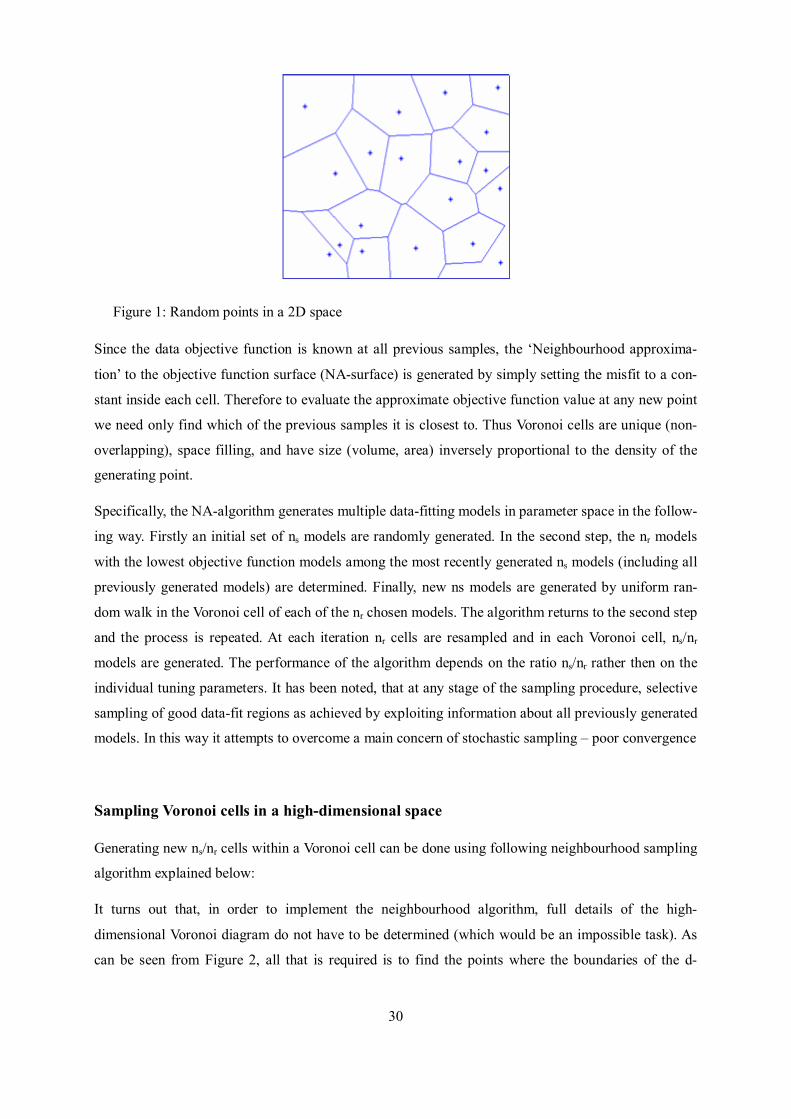
Given n points in a plane, their Voronoi diagram divides the plane according to the nearest neighbour

rule namely, each point is associated with the region of the plane closest to it. The distance metric is

usually Euclidian, and each Voronoi polygon in the Voronoi diagram is defined by a generator point

and a nearest neighbour region, see Figure 1

30

Figure 1: Random points in a 2D space

Since the data objective function is known at all previous samples, the ‘Neighbourhood approxima-

tion’ to the objective function surface (NA-surface) is generated by simply setting the misfit to a con-

stant inside each cell. Therefore to evaluate the approximate objective function value at any new point

we need only find which of the previous samples it is closest to. Thus Voronoi cells are unique (non-

overlapping), space filling, and have size (volume, area) inversely proportional to the density of the

generating point.

Specifically, the NA-algorithm generates multiple data-fitting models in parameter space in the follow-

ing way. Firstly an initial set of ns models are randomly generated. In the second step, the nr models

with the lowest objective function models among the most recently generated ns models (including all

previously generated models) are determined. Finally, new ns models are generated by uniform ran-

dom walk in the Voronoi cell of each of the nr chosen models. The algorithm returns to the second step

and the process is repeated. At each iteration nr cells are resampled and in each Voronoi cell, ns/nr

models are generated. The performance of the algorithm depends on the ratio ns/nr rather then on the

individual tuning parameters. It has been noted, that at any stage of the sampling procedure, selective

sampling of good data-fit regions as achieved by exploiting information about all previously generated

models. In this way it attempts to overcome a main concern of stochastic sampling – poor convergence

Sampling Voronoi cells in a high-dimensional space

Generating new ns/nr cells within a Voronoi cell can be done using following neighbourhood sampling

algorithm explained below:

It turns out that, in order to implement the neighbourhood algorithm, full details of the high-

dimensional Voronoi diagram do not have to be determined (which would be an impossible task). As

can be seen from Figure 2, all that is required is to find the points where the boundaries of the d-

31

dimensional Voronoi cell intersect the i-th axis passing through a given point A. The next step of the

uniform random walk is restricted to lie between these two points on the axis (i.e. xj and xl in Figure 2)

Figure 2 A uniform random walk restricted to a chosen Voronoi cell

After following refined approach the exact intersection of axis can be calculated. If we define the k-th

Voronoi cell at the one about sample vk, and the point where the boundary between cells k and j inter-

sects the axis xj (Figure 2), then by definition we have

( ) ( )jjjk xvxv −=− (2.34)

or

( ) ( )2,,

22,,

2ljljjljlkk xvdxvd −+=−+ (2.35)

Where kd is the perpendicular distance of sample k from the current axis, and a subscript of l denotes

the i-th component of the corresponding vector. Solving for the intersection point we obtain.

( )( )

−−

++=ljlk

jkijikij vv

ddvvx

,,

22

,,, 21

(2.36)

To find the required boundaries of the Voronoi cell, the above equation must be evaluated for all np

cells and the two closest points either side of A retained. More formally, we have the lower boundary

given by

[ ] ),,1;(,,max ,.. plAljlji njxxforxl K=≤ (2.37)

and the upper boundary given by

32

[ ] ),,1;(,,max ,.. plAljlji njxxforxu K=≥ (2.38)

Where il and iu are the lower and upper bounds of the parameter space in the i-th dimension, respec-

tively. To complete the description we need the set of squared perpendicular distances,

( )pj njd ,,12 K= available at each step of the walk. These can be calculated for the initial axis and

for new axis by a recursive update procedure. For example, after the i-th step has been completed and

the work moves from A to B, the current set of 2jd values can be calculated for the (i+1)-th axis using

( ) ( ) ( ) ( ) ( )piBijiBijijijnjforxvxvdd ,,12

1,1,2

,,2

12 K=−−−+= +++

(2.39)

Thus, using the NA-Algorithm we can effective evolve a non-linear dynamical system, test the inverse

problem in terms of non-uniqueness and once an acceptable history match or solution is obtained, the

local optimization methods (gradient-based approaches) can be used to fine tune the process, i.e. to

find the nearest optimum near any point in the search space which provides results close to an accept-

able solution. At the end of model calibration procedure, on the basis of sensitivity analyses, the Inter-

pretation of the Parameter Estimates and Uncertainty Quantification can be evaluated.

33

2.3.3 Analyses of Parameter Estimation Uncertainties

The best estimate parameter set Θ is determined by matching the model to a measured data set. Due

to the random nature of the observed values, the identified parameters are always associated with un-

certainties and thus the analysis of the estimation errors is a further important aspect of model calibra-

tion. The goal is to find an approximation of this probability distribution despite the fact that the true

parameter vector Θ~ is unknown, and that only one data set is available for inversion.

Under the assumption that the relation between the observed data and the model parameters can be

linearized around the maximum likelihood solution, then we could express the vector obsu as:

ε+Θ= ΘJuobs (2.40)

For this approximated models, ΘJ is the sensitivity or Jacobian matrix (Nm x Np) computed at Θ and

ε represents the random error.

Under the assumption of normality, the joint probability distribution of the parameter estimates is fully

described by their mean and covariance matrix. The covariance matrix of the estimated parameters,

)ˆ( MCov Θ , contains the standard error or uncertainties of the estimate Θ , as well as covariances,

which describe the statistical correlations between pairs of parameters. This matrix can be evaluated

using following relationship:

( )( ) ( )( )

Θ−ΘΘ−Θ=Θ

TEEEMCov ˆˆ)ˆ( (2.41)

The necessary condition for the minimization of generalized last squares after Equation 2.22 gives

( ) ( ) 01 =Θ−−=Θ∂

Θ∂ − JuCovJOF obsTε (2.42)

Thus, the estimated parameter can be solved as

obsuB=Θ (2.43)

Where

( ) 111 −−−= εε CovJJCovJB TT (2.44)

Replacing Θ with the following equation in the Equation 2.41 yields:

34

( ) ( )[ ]( ) 11

)ˆ(−−==

Θ−Θ−=Θ

JCovJBCovB

BJuJuEBMCovTT

TTobsobs

εε

(2.45)

In the case if the statistical parameters in covariance matrix 1−εCov are unknown, they may be esti-

mated together with the unknown model parameters Θ by the following two-stage iterative procedure

(Carrera and Neuman, 1986b).

In the first stage, the model parameters are estimated by the generalized last square method, where the

covariance matrix of measured values is given by their initial guess. In the second stage, the maximum

likelihood method is used to estimate error variance, where the parameter vector is replaced by the

values just obtained in the first stage. The two stages are then iterated until a convergent criterion is

satisfied.

The variance-covariance matrix for the final estimated parameters is given by:

[ ] 120)ˆ( −⋅=Θ JJsMCov T (2.46)

where, 20s is the calculated error variance as a measure of goodness-of-fit :

( )pm NNMOF

s−Θ

=ˆ

20 (2.47)

The evaluated covariance matrix )ˆ( MCov Θ for the model M can be used for the error analyses for

the estimated parameters and it can provides a criterion for the selection of an appropriate parameter-

ized model which must weigh the trade-off between increased information and decreased reliability.

Since, by increasing the number of parameters we can always improve the overall fitting of the model,

this match comes at the expense of a reduction in model reliability (Uncertainty of the estimated pa-

rameters may grow rapidly due to the decrease of ( )pm NN − or due to the correlation effects caused

by large number of estimated parameters). Therefore this relationship gives an explanation of the over-

parametrization problem.

35

2.3.4 Optimality and Model Identification Criteria

If numerical reservoir models have been developed and matched to the data, a criterion is needed to

decide which of the alternatives is preferable. A number of tests for model discrimination have been

developed as described by Steinberg and Hunter [1984], Carrera and Neuman [1986a], and Russo

[1988], Russo et al. [1991]. One of the most used criteria is the estimated error variance as a measure

of goodness-of-fit (Equation 2.47). The model that best matches the data is considered to be the best.

However, since the match can always be improved by adding more fitting parameters, the goodness-

of-fit is an inappropriate basis for model selection because it almost always leads to overparameteriza-

tion. Overparameterization means that an improvement of the fit comes at the expense of a reduction

in model reliability. Increasing the number of parameters also increases the correlations among the

parameters, which results in higher estimation uncertainties if the match is not significantly improved.

Consequently, model identification and optimality criteria should include some aggregate measure of

overall estimation uncertainty to guard against overparameterization.

The selection of an appropriate parameterized model would be objective and one would like to have as

good an approximation of the structure of the system as the information permits. The goal is to find a

model for the given measured data set that is best in the sense that the model loses as little information

as possible. This thinking leads directly to the concept of Kullback-Leibler information (the measure

of departure of the model from the true system), which provides the theoretical basis for the method-

ology of choosing the best parameterized reservoir model explained below. The applicability of alter-

native statistical model selection approaches, such as Akaike’s, Schwarz’s and Kashyap criteria are

also tested.

2.3.4.1 Kullback-Leibler Information

The method of measure the Kullback-Leibler (K-L) “distance” between two models is derived from

information theory and is discussed by Burnham and Anderson, 1998. This is a fundamental quantity

in the sciences and has earlier roots in Boltzmann’s concept of generalized entropy in physics and

thermodynamics.

Here are introduced some general notations. We use x to denote the data, which arise from full reality

and can be used to make formal inference back to this truth. The f and g are notations for a full

reality and an approximating model respectively, in terms of probability distributions. The K-L dis-

tance between truth f and model g is defined for these continuous functions as the (usually multi-

dimensional) integral:

36

( ) ( ) ( )( ) dxxgxfxfgfI

= ∫ θ

log, (2.48)

where log denotes the natural logarithm and Θ represents generally a parameter or parameter vector

of the model g . The Notation ( )gfI , relates to the information lost when model g is used to ap-

proximate truth f . Since, we seek an approximating model that loses as little information as possible;

this is equivalent to minimizing ( )gfI , over the models in the set. An interpretation equivalent to

minimizing ( )gfI , is that we seek an approximating model that is the “shortest distance” away from

the truth. The K-L Distance ( )gfI , is always positive except when the two distributions f and g

are identical (i.e. ( ) 0, =gfI if and only when )()( xgxf = ). The K-L distance defined above can

be written equivalently as a difference between two expectations with respect to the distribution f :

( ) ( )( )[ ] ( )( )[ ] ( )( )[ ]θθ xgEconstxgExfEgfI fff log.loglog, −=−= (2.49)

Knowing the K-L distance for different models ig , one can easily rank the models from best to worst

within the set of candidates, using the differences ( i∆ ) of the K-L values. This allows the ability to

assess not only a model rank, but also whether the j-th model is nearly tied with the i-th model or is

relatively distant (i.e. corresponding to a large loss of information). For the prediction purposes of the

model, it is often unreasonable to expect to make inferences from a single (best) model. As suggested

by Akaike, 1978, the model selection uncertainty can be quantified by calibrating the relative plausi-

bility of each fitted model ( iM ) by a weight of evidence ( iω ) as being the actual best K-L model.

This can be done by extending the concept of the likelihood of the parameters given both the data and

model, i.e., ( ) ( )Θ=Θ xgMxL ii, , to a concept of the likelihood of the model given the data, hence

( )xML i :

( ) ( )ii xML ∆−∝ exp (2.50)

To better interpret the relative likelihood, we normalize the above relationship to be a set of positive

K-L weights, iω , summing to 1:

( )( )∑

=

∆−

∆−= R

rr

ii

1

exp

expω (2.51)

where, R is the number of alternative models. Drawing on Bayesian ideas, it seems clear that we can

interpret iω as the estimated probability that model i is the K-L best one for the data at hand, given

37

the set of models considered. These weights are very useful to translate the uncertainty associated with

model selection into the uncertainty to assess the model prediction performance.

Use of the Kullback-Leibler concept for the predictive model

As stated above in the chapter 2.2.1 the estimated parameters are always associated with uncertainties

and the evaluated parameter covariance matrix )ˆ( MCov Θ for the model M can give a basis for a

quantitative measure of model reliability. The uncertain parameters on its part influences the uncer-

tainty for the future production performance. According to the linear perturbation analysis, this can be

quantified by the following assumption:

[ ] [ ] Tpred AMCovAMuCov ⋅Θ⋅= )ˆ()( (2.52)

where, [ ]A is the matrix of sensitivities of the predicted values.

The diagonal elements of matrix )( MuCov pred equal the variances 2

iipredσ of the predicted quan-

tity. The whole uncertainty 2ip

σ of this value must include also the effects of measurement error that

is likely to be incurred if the predicted quantity were to be measured:

222iiii measpredp σσσ += (2.53)

Based on this statement, we measure the K-L distance or the “information lost” (Equation 2.48) be-

tween the real system responses, expressed by the normally distributed random values

( )2,imeas

measnuN σ and the underlying approximated model ( )2,

ipprednuN σ . This procedure can be ap-

plied chronologically at each time step n and the evaluation of the appropriate K-L distance is based

on the match to the first (n-1) observations. The calculated “distance” becomes more and more signifi-

cant to the data values observed at the last time steps.

This methodology ranks and weights the approximated alternative models in regard to the “distance”

away from truth. In other words, it prefers the models that predict the real system responses more ac-

curately than other alternative ones and with lower uncertainty 2iipredσ . Thus, it takes into account the

tradeoff between squared bias and variance of parameter estimates, which is fundamental to the prin-

ciple of parsimony.

38

2.3.4.2 Alternative Model Selection Criteria

In addition to the above presented methodology, we analyze the applicability of other widely applied

statistical model selection approaches. The first criterion (AIC - Akaike Information Criterion) is that

developed by Akaike, 1973. This method intends to estimate the relative Kullback-Leibler Informa-

tion. After some simplifying assumption it leads to:

pmeas NuLAIC 2)]ˆ([ln2 +Θ−= (2.54)

where, pN is the dimension of parameterization. The AIC has a drawback - as the sample size in-

creases there is an increasing tendency to accept a more complex model. The Bayesian Information

Criterion - BIC (derived by Schwarz 1978) takes the sample size into account. This method tries to

select model that maximizes the posterior model probability and is given by:

mpmeas NNuLBIC ln)]ˆ([ln2 +Θ−= (2.55)

The third criterion to be discussed is the one derived by Kashyap, 1982, which minimizes the average

probability of selecting the wrong model among a set of alternatives:

( ) HNNuLd mpmeas

M ln2ln)]ˆ([ln2 ++Θ−= π (2.56)

where, H is the Hessian matrix.

39

2.3.5 Application to the Synthetic Field Example

The application of the above presented methodology is demonstrated on the PUNQ–project (= produc-

tion forecasting with uncertainty quantification). This is a synthetic test example, based on a real field

case. The original aim of this project were to compare a number of different methods for quantifying

the uncertainty associated with their forecast when historical production data is available, and to pre-

dict the production performance (the cumulative oil production after 16,5 years) for a given develop-

ment scheme. We confine ourselves here to the presentation of model selection results and, addition-

ally, we predict the oil recovery based on the inference from the entire sets of matched models. A

complete description of how the truth PUNQ-case was generated has been prepared by Frans Floris of

TNO, 2000. All of the data was extracted from the TNO web site [http://www.nitg.tno.nl/punq/].

2.3.5.1 Reservoir Description and Parameterization

In brief, the reservoir model contains 19x28x5 grid blocks of which 1761 are active. The grid blocks

are 180 meters square in the areal sense. Figure 3 shows the top surface map and the well positions.

There are six producing wells located near the initial gas-oil contact. A geostatistical model based on

Gaussian random fields has been used to generate the porosity/permeability distribution. Figure 4

shows the distribution of horizontal permeability in three of the five layers for the “truth case”. The

production period includes one year of extended well testing, three years of shut-in and then 12.5 years

of field production. Simulated production data for the first 8 years, including pressures, water cutes

and gas-oil ratios for each well, were available and Gaussian noise was added to represent the meas-

urement errors. The noise level on the bottom-hole pressure (BHP) was assumed at 2% of the actual

value, the standard deviation of the measurement error on the gas-oil-ratio (GOR) at 5% and the same

noise level was taken for water cuts. Besides some geological knowledge, the measurement “preci-

sion” and the observed data itself is assumed as being the basis information extracted from the “truth”.

Using K-L theory we seek an “best parameterized” model, that has the “shortest distance” to this

measured system.

It is assumed, that the generated model has uncertainties associated with permeability (horizon-

tal/vertical) and porosity distributions as well as the initial gas-oil ratio. All other model parameters

(structure, PVT, rel. perms, etc) are assumed to be known. A prior reservoir model is inferred from the

rough geological description and is used to construct the initial model before any history matching

procedure. Since in real cases we have limited knowledge about the real geological system (such as

size and shape of sedimentary bodies, structural trends and styles), we made reasonable assumption

about the geostatistical parameters, such as means and variograms for the porosity and permeability

values, to be consistent with the basis reservoir model. Different anisotropy directions within the vari-

40

ous layers are averaged out for the entire domain. In this example, the variogram used has a longer

range in the NW-SE directions for the good reproduction of the main trend of the parameter variations.

The well points are fixed and the initial properties (porosity and horizontal/vertical permeabilities) are

interpolated using the kriging procedure.

The next step is to parameterize the kriged fields, taking into account both local dependencies of res-

ervoir properties and the high sensitivities and low correlation among the defined regional parameters.

The first requirement is achieved through the use of multiplier factors for the porosity and permeabil-

ity values rather then the rock properties themselves. The second problem is solved by means of the

gradzone analyses suggested by Bissell, 1994 for selecting the zone in a reservoir model where the

multiplier factor may be applied. For these purposes the eigenvector-eigenvalue analyses of the Hes-

sian matrix is used for each parameter type. The sensitivity analysis for parameter selection and calcu-

lation of analytic gradients was performed using the commercial software ECLIPSE. This parameteri-

zation method takes into account both the good regression performance of the minimization problem

and the constraints imposed by geology. That is, the pore volume or the permeability (horizon-

tal/vertical) of all gridcells in a gradzone is multiplied by a common factor (MULTPV and

MULTXY/MULTZ respectively). Thus, the gridcells in one gradzone can have different properties but

their values relative to each other remain constant as the multiplier is changed.

2.3.5.2 Simulation Results

The “history match” procedure with the gradient-based optimization approach was applied for alterna-

tive models with different zonation structures. Table 1 lists the models with appropriate regional pa-

rameter sets. In addition to the gradzone method there are also the simple models with the multiplier

parameters for each layer or for the whole reservoir domain. (Models 1, 10-13). In Figure 5 the

“measured” production data, in terms of gas-oil ratios and bottom-hole pressures, are compared with

the optimized simulation results for the well “PRO-4” (model 6*). It must be noted that with the other

parameterization structure of the model the visual match did not significantly improve. Only model 1

leads to relatively poor history matches. Generally, the use of the Kullback-Leibler concept for model

selection can be applied at each time step. In which, we use all data from the start point to the one

currently under investigation to predict the model responses at the next time step. The estimated pa-

rameter values must be updated at each time step, but this procedure is very time consuming. Instead,

it would be reasonable to guess how far “into the future” we can trust the model and make a predic-

tion. In this example, we assume that the values of the final calculated parameters remain constant for

the last 2 years of the production period, which includes the last 10 observed time steps. Only the vari-

ance-covariance matrix will be affected by the adding of sensitivity coefficients up to the current point

in question. On this basis the next production data will be predicted and the associated uncertainty

41

evaluated. Afterwards, the calculated quantity will be compared with measured data with regard to the

bias and the variance using the Kullback-Leibler “distance”(Equation 2.49). The integral is calculated

numerically. The K-L distance for each time step from the last 2 years production is shown in Table 2

The results at every time point are averaged over three data values. Model 6* is superior to the other

ones, which on a basis of measured data maximizes the reliability of model predictions as a result of

minimizing the uncertainty of estimated parameters.

The additional results to rank the alternative models are given in Table 3. This table lists the calculated

objective function (OF), the three model selection criteria (AIC, BIC, dm) with regard to the principle

of parsimony (the minimum values indicate the “well parameterized” model) and the K-L weights for

each of the alternative models referred to the last time point. The overall ranking of the models shows

the different behaviours for each of the applied approaches. The AIC and BIC indexes, unlike the dm

criterion, have a tendency to accept a more complex model for large number of observations. For the

Kashyap criterion the limit of the overparametrization is already achieved with model 5, which in-

cludes seven estimated regional parameter values. Furthermore, based on the calculated K-L weights

we make formal inference from the entire set of models for model prediction purposes. It is desirable

for this particular case, since no single model is clearly superior to some of the others in the set. De-

spite the fact that all patterns matched the production data very well, the predicted quantity (the cumu-

lative oil production (FOPT) after 16,5 years) differs across the models as shown in Figure 6. There-

fore, it is risky to base prediction on only the selected model. An obvious possibility is to compute a

weighted estimate of the predicted value. According to the concept of averaging (Equation 2.51) this

can be calculated as follows:

∑=

⋅=R

iii FOPTFOPT

1

ω (2.57)

The model selection uncertainty is also included when measuring the uncertainty for the predicted

values:

2

1

2)()(var)(var

−+⋅= ∑=

R

iiii FOPTFOPTFOPTFOPT ω (2.58)

where, R is the number of models and )(var iFOPT is the variance of the cumulative oil production,

calculated using linear uncertainty analysis for the i-th fitted model. The result is shown in Figure 6 as

model 14.

Thus in this chapter the statistical model selection approaches, based on the Kullback-Leibler informa-

tion, were used to choose the best parameter zonation pattern for a reservoir model. The discrepancy

with other model selection criteria results from the direct measure of model departure from the true

system, taking into account the bias and variance between the predicted and observed system re-

42

sponses. Thus, this approach balances the trade-off between increased information and decreased reli-

ability, which is fundamental to the principle of parsimony. In the case where no single model is

clearly superior to some of the others, it is reasonable to use the concepts for model averaging for

translating the uncertainty associated with model selection into the uncertainty to assess the model

prediction performance.

43

Table 1: The set of different parameterized models

Number of Parameters

Initial GOR MULTXY MULTZ MULTPV

Model 1 1 1 1 1

Model 2* 1 2 1 1

Model 3* 1 3 1 1

Model 4* 1 2 1 3

Model 5* 1 2 3 1

Model 6* 1 4 1 1

Model 7* 1 3 1 3

Model 8* 1 3 3 1

Model 9* 1 2 3 3

Model 10 1 5 5 1

Model 11 1 5 1 5

Model 12 1 1 5 5

Model 13 1 5 5 5

* - Indicates the models parameterized by gradzone method

Table 2: Ranking the models with the K-L distance

The calculated Kullback-

LeiblerDistance

2206

day

2207

day

2373

day

2557

day

2558

day

2571

day

2572

day

2738

day

2922

day

2923

day

2936

day

Model 1 0.176 6.942 11.258 4.403 1.201 0.749 4.214 4.727 11.992 2.708 2.009

Model 2* 0.080 4.982 5.860 4.206 0.282 0.166 7.476 10.43 8.969 0.814 0.562

Model 3 * 0.081 5.193 5.460 5.635 0.278 0.171 6.978 9.210 8.613 0.817 0.584

Model 4* 0.177 5.040 6.163 5.758 1.269 0.141 5.719 8.549 7.708 0.620 0.423

Model 5* 0.068 3.647 8.335 7.036 0.280 0.141 7.944 11.00 9.996 0.810 0.507

Model 6* 0.083 6.414 2.908 1.749 0.109 0.073 3.801 4.186 4.620 0.445 0.348

Model 7 * 0.154 5.464 6.122 7.689 0.319 0.157 5.820 7.655 7.455 0.638 0.471

Model 8* 0.073 4.280 4.884 5.258 0.334 0.147 5.971 7.610 10.052 0.785 0.490

Model 9* 0.242 5.358 5.124 4.370 0.413 0.205 4.764 5.232 5.322 1.097 1.429

Model 10 3.085 3.298 3.409 3.848 0.183 0.153 2.814 4.433 5.080 0.393 0.461

Model 11 0.627 11.57 3.978 4.876 1.658 2.323 4.477 6.190 10.117 3.230 2.657

Model 12 1.249 11.65 5.725 4.577 0.192 0.415 4.789 6.406 7.344 0.474 1.885

Model 13 1.162 6.464 5.607 4.220 0.279 0.617 3.375 5.088 6.029 0.451 0.631

44

Table 3: Ranking the models with different model selection criteria

Number of

Parameters OF AIC BIC dm K-L weight

Model 1 4 1211.2 3708.13 3724.82 3747.83 0.022

Model 2* 5 701.05 3199.98 3220.85 3242.57 0.094

Model 3 * 6 699 3199.93 3224.97 3251.41 0.092

Model 4* 7 689.51 3192.44 3221.66 3245.49 0.108

Model 5* 7 650.46 3153.39 3182.61 3201.56 0.099

Model 6* 7 652.55 3155.48 3184.70 3208.64 0.116

Model 7 * 8 686.33 3191.26 3224.65 3245.69 0.103

Model 8* 8 647.26 3152.19 3185.58 3215.45 0.101

Model 9* 9 655.87 3162.80 3200.36 3232.53 0.039

Model 10 12 621.5 3134.43 3184.51 3225.53 0.104

Model 11 12 688.99 3201.92 3252.00 3288.17 0.012

Model 12 12 640.78 3153.71 3203.79 3233.50 0.025

Model 13 16 601 3121.93 3188.71 3220.82 0.087

Figure 3: Top Structure map of the PUNQ case with well locations (from Floris et al. )

45

Figure 4: Truth case: Horizontal permeability fields for layers 1, 3, 5

Figure 5: The production data for the well “PRO-4”

Figure 6: The prediction results

46

3 Simulation of the Production Behavior of Hydrauli-

cally Fractured Wells in Tight Gas Reservoirs

Tight gas reservoirs bear large resources of gas all over the world. Due to their very low matrix per-

meability, the production from these formations is usually below an economical limit. Therefore, hy-

draulic fracturing is often essential to stimulate the gas production to economical reasonable rates. The

Experiences show that the post-fracture productivity is frequently lower than predicted. Deficits in the

simulation models and their applicability for tight formations can be considered as major reasons for

that. Hence, customization of the simulation techniques regarding the specific conditions for the hy-

draulically fractured wells and identification of typical damage mechanisms is the major objective of

this work.

For more plausible evaluation of hydraulic fracture stimulation and for more realistic forecasts of the

post-fracture well performance, an accurate representation considering the flow in the immediate frac-

ture environment becomes a necessity. In terms of numerical simulation of fractured well production

behaviour, the problem can be addressed by (i) an adequate representation of the fracture in a reservoir

simulator, and (ii) a reasonably accurate picture of the initial fluid distribution around the fracture after

the treatment process. This modelling step gives a basis for the further numerical investigations and

analyses of damage mechanisms typically occurred in context of the stimulation treatment. Particular

attention is also given the investigations of clean up process following the leakoff in the course of the

stimulation and the conditions were determined where hydraulic and mechanical damage impair pro-

ductivity.

To ease the workflow of hydraulic fracture simulation by automatically setting up an appropriate simu-

lation model, a support tool was developed which provides the coupling of commercial fracturing

software with reservoir simulators. The tool integrates both the detailed geometry of the fracture as

well as the saturation conditions after the leakoff. The tool is applicable to an arbitrary fracture con-

figuration scenario with any number of fractures and a flexible well path. The reason for writing a

special support code was, apart from the apparent need for saving the user’s time and effort, to incor-

porate the reservoir simulator into inverse algorithm to perform automatic history matching. In such a

system, an additional interface module is needed to update a simulation model at each varying the

parameters to be identified. Thus, the availability of the support tool to integrate hydraulically frac-

tured wells into reservoir simulation model facilitates both model calibration as well as production

optimization. The usage is illustrated by history matching as well as by the production optimization

example of multiple fractured well within a Rotliegenden tight gas formation in Northern Germany.

47

3.1 Introduction to Fractured Well Simulation

Historically, there have been three basic approaches commonly used for predicting the production

from hydraulically fractured wells. First, analytic solutions were most commonly used, based on an

infinite conductivity or later a finite conductivity fracture with a given half-length. This approach was

also extended to cover horizontal multiple fractured wells (Basquet, 1999). With the development of

reservoir simulators, two other approaches were developed.

For complicated multi-well, multi-layer, multi-phase simulations (i.e. full field models), the fracture

stimulation was usually approximated as a negative skin. This is the same as increasing the effective

wellbore radius in the simulation model. An alternate approach, developed initially for tight gas appli-

cations, was to develop a special purpose numeric reservoir simulator which could explicitly model

the flow in the fracture and take into account the special properties of the proppant, such as the stress

dependant permeability or the possibility of non-Darcy flow. Such models typically were limited to a

single layer, single-phase (oil or gas) situation.

More recently, with the advent of faster computers with sufficient memory, it became feasible to avoid

the compromises that were made in the past when trying to model hydraulic fractures with a normal

3D reservoir simulator. Initially, people manually built grid refinement into their reservoir models to

represent a hydraulic fracture (Ehrl E., Schueler, S., 2000). Although this method works fine, it is very

time consuming for the engineer, because complicated gridding schemes are necessary to correctly

represent the fracture geometry. In addition, the detailed description of the fracture properties from a

fracture simulation was not usually passed through to the reservoir model, resulting in the assumption

of constant properties (i.e. permeability) for the fracture. This method of simulation is not very effi-

cient and can lead to inconsistencies in the data used in the different simulations.

In the paper (Friedel et al. 2002) is given a comprehensive comparitive analysis of different ap-

proaches to numerical modeling of the fractured wells in tight reservoirs. Among them were 1) frac-

ture considered by a series of high-permeability gridblocks of a reservoir model, 2) separated reservoir

and fracture models coupled through the source/sink term, and 3) fracture presented by modification

of the transmissibilities of the reservoir gridblocks containing the fracture. It was shown that the first,

more traditional technique with a reasonably local grid refinement, can be the preferred method when

the flow understudy does not contain any features, making it difficult to simulate within the frame-

work of a reservoir model. So, the present work was oriented to the use of a conventional reservoir-

simulation program.

The integration of the fracture into the reservoir model is not a problem of great concern. A short dis-

cussion of this may be found in Settari et al. (1990) and Banerjee et al. (2004). Because of the time-

step limitation and because of Peaceman’s condition for structured orthogonal grids, the fracture in the

model can not take the actual width. Correspondingly, the permeability and porosity of the fracture

48

blocks are reduced to maintain the transmissibility and porous volume of the fracture. The starting

values of the hydraulic parameters within the fracture are calculated from the proppant distribution

after the closure. These data can be obtained through the fracturing simulation in consideration of

proppant-transport processes or indirectly through geophysical measurements.

Another important point is the consideration of conditions in the hydraulically damaged fracture envi-

ronment after closure and how to integrate them into a reservoir-simulation mode. During the fractur-

ing process, a large volume of technical fluid is injected into the reservoir utilizing high pressure and

high flow rates. As soon as the fluid is in contact with the rock, some of it leaks off along the fracture

face into the formation. After the pumping is stopped, the remaining low viscous fracturing fluid still

imbibes into the formation due to the capillary forces and overpressure in the fracture. Eventually,

after the treatment is finished, an invaded zone around the fracture will be formed. The extent of that

zone depends, e.g., on the exposure time of the fluid to the formation, as well as fluid and reservoir

properties. The saturation conditions in the invasion zone are responsible for the occurrence of hy-

draulically induced damage (so called phase trapping), either by capillary forces or adverse relative

permeability effects, as well as a combination of both. Those functions may have considerable impact

on the cleanup behaviour of a fractured well. In contradiction to conventional gas reservoirs, they are

distinctly different in tight formations, which can affect the characteristics of the well significantly

[Bennion et. al 2000]. The capillary pressure is inversely proportional to the pore radius. Hence, capil-

lary forces act stronger in tight formations, where effective pore radii are small [Penny et al, 1983]. It

is characteristic of low permeability gas reservoirs to have a poor single- phase water permeability, 3

to 10 times smaller than that of the rock permeability. In the presence of a gas phase, the waters rela-

tive permeability is further decreased. That is a reason for a strong decline of the water phase mobility

during cleanup.

The limited water mobility and the capillary forces imply that: (i) the load water of the fracturing fluid

can not be drained completely from the gas phase, and (ii) the gas relative permeability is permanently

lowered due to the water retained in the invasion zone. Holditch, 1979 investigated factors affecting

water blocking and the gas flow from fractured wells using numerical simulation. He stated that the

gas flow can even be blocked totally if the drawdown pressure does not exceed the capillary pressure

in the invaded zone. This is particularly the case if permeability in the invaded zone is impaired as a

consequence of so called mechanical damage. In the course of the fracturing treatment, the permeabil-

ity within the immediate fracture vicinity may be severely reduced. That usually implies tremendous

capillary forces and, thereby, an accumulation of water in the mechanical damage zone causing addi-

tional flow resistance for the gas phase.

A variety of numerical studies have been published in the past that focused attention on the cleanup or

water-blockage analysis. First, the distribution of invaded fluid in the fracture vicinity can be obtained

as a result of the numerical modeling of the fracture treatment. In the special fracture simulators de-

49

veloped, for example, by Settari (1980) and Nghiem et al. (1984), a fracture-mechanics model is cou-

pled with the fracture and reservoir two-phase flow (filtrate assumes the properties of the reservoir

water) equations. These imply the mass exchange between the fracture and formation on the basis of

Darcy’s law. Thus, the formation of the invaded zone during the fracture propagation is described by

the general theory of the flow in porous media. The peculiar conditions on the fracture surface (e.g.,

deposition of the filtercake) and the features of the fluid properties necessitated a special model for the

flow of fracturing fluid into the reservoir. In the classical leakoff theory, the flow rate varies inversely

with the square root of the time. The factor of proportionality (i.e., the leakoff coefficient) is a charac-

teristic of the formation and the fracturing fluid. On this ground, other fracture modeling algorithms

(Howard and Fast 1970) were developed in which the fracture-propagation model is solved independ-

ently of the reservoir equations. However, such approaches are not aimed at providing the solution for

the saturation profile in the invaded zone.

On the basis of his generalized leakoff model, Settari et al. (1990) has suggested a partially decoupled

modeling of the fracturing processes, whereby, processes in the formation are taken into account but in

a manner that does not require numerically solving the reservoir model. The flow through the invaded

zone is considered as a piston-like displacement (with some correction for two-phase flow effects). So,

an idealized uniform saturation profile in a normal direction to the fracture surface builds up. The

problem of estimating the fluid distribution in the damage zone implies a radically different way of

handling when the modeling is focused upon the post-fracture well performance only. In this case, it is

assumed that the monitored data concerning the fluid and proppant injection during the fracture treat-

ment and geometry parameters of the stationary fracture are available. In a typical—and the sim-

plest—approach, the entire amount of invaded fluid, calculated from the material balance, is placed in

the fracture’s surrounding region (Tannich 1975; Bastian and Sherman 1993). In doing so, the depth of

invasion can depend on the porosity, net thickness value, and reservoir water saturation and can be

correlated with the fact that near the well the formation is exposed to the fracturing fluid for a longer

time. To create more proper saturation profiles along the fracture, the modeling of hypothetical water

injection into the existing, but undamaged, fracture can be performed (Sherman and Holditch 1991).

An advantage of this approach is that immediate transition to further simulation of the post-fracture

production is provided. At the same time, replacing the fracturing process with a fictive water injection

can be a mistake on many points. For example, the time the water front takes to arrive at a specified

location of the fracture (i.e., reduction of the maximum possible exposure time of water to formation)

depends heavily on the fracture conductivity.

In this work is shown a new way (presented by Behr et al., 2002) to estimate the fluid distribution in

the damage zone after the fracturing treatment. The idea is 1) to reconstruct the prehistory by a simpli-

fied fracture propagation model, 2) to extract from its solution the data on distribution of the leakoff

time and leakoff coefficient over the fracture, and 3) to calculate the more realistic saturation profiles

50

around the fracture using a two-phase flow model. The propagation model retains the simplicity of the

classical leakoff theory, although it is more comprehensive and potentially more accurate than other

methods, estimating the fluid loss without resorting to a fracture simulator. The flow model, in contrast

to piston-like displacement, takes account of the relative permeability phenomena. At the same time,

the model is very convenient to use because it allows a self-similar structure of the saturation profile,

hence, only one semi-analytical solution, universal for a specific type of the formation rock, has to be

calculated to determine the fluid distribution in the damage zone.

3.2 Automatic Generaton of the Simulation Model for Frac-

tured Wells

The developed algorithm including the fracture and damage presentation was implemented in the in-

house tool to automatically prearrange the input file of a commercial reservoir simulator and to pre-

pare the reservoir model for the post-fracture simulation. The reason for writing a special support

code, apart from the apparent need to save the users time and effort, was to incorporate the reservoir

simulator into an inverse algorithm to perform automatic history matching of the production behaviour

of hydraulically fractured well.

The tool serves the following three functions:

1. To introduce proper local refinement into the reservoir grid in the fracture environment.

2. To integrate the geometry and properties of fracture into the simulation model.

3. To initialize the model with respect to the fluid saturation around the fracture.

In the following, are explained some details of these functions.

51

3.2.1 Local Grid Refinement

The motivation behind the grid creation algorithm is (i) to adapt the grid to the geometry of the reser-

voir, layers and fractures as well as to the flow around the fractures and (ii) to have an optimal number

of gridblocks in terms of minimum storage space/CPU time versus required accuracy of the simula-

tion.

The procedure of creating the local grid refinement implies four main steps:

1. Specifying the refinement domain within the host grid on the base of location and extent of the

fractures.

2. Primary domain refinement (Figure 7). A typical scale of spacing is specified by definition of re-

finement factor for the gridblock of a maximum size.

Figure 7: Primary refinement of fracture

3. Secondary refinement in the grid blocks containing the well or one of the fractures (Figure 8).

Here, three possibilities of discretising are provided: (i) uniform refinement; (ii) logarithmic refine-

ment, where the distance of the grid lines to the center of refined block, or fracture face, increases with

a fixed ratio to that of preceding grid line; (iii) geometric progression for the gridblock sizes, i.e., the

sizes of the neighbouring grid blocks are in the same ratio. The number refinement blocks within the

block of primary refinement can either be specified by user or be calculated by the code to best satisfy

a chosen principle of discretization. The width of the grid blocks responsible for the fracture presenta-

tion is considered as extra parameter for the secondary refinement.

4. Preparing the ECLIPSE input files providing the introduction of designed LGR into the reser-

voir model.

52

Figure 8: Secondary refinement of well and fracture

53

3.2.2 Integration of the Fracture Parameters

The typical output from the fracturing-process analysis contains the following information regarding

the fracture characteristics:

• Surface proppant concentration (mass per unit area of fracture surface):

bc p ⋅= ρ (3.1)

and/or

• fracture conductivity

bkFc ⋅= (3.2)

Figure 9 illustrates the distribution of these parameters by the elliptical zones in one example. Pro-

vided that the properties of the proppant pack do not vary spatially, these quantities contain the same

information as the propped-fracture width, b.

The fracture is represented in the reservoir model with a fictive width, bf, (Figure 9), which is the size

of the corresponding gridblocks. Because the porous volumes and the transmissibilities of the fracture

blocks are to remain unchanged, the porosities and permeabilities in the fracture gridblocks should be

recalculated:

fpf

f

cf b

cbF

k⋅

==ρ

φφ, (3.3)

Here, the equality of the fracture porosity, φ , and proppant-pack porosity, pφ , is assumed. In a more

general case, the proppant distribution in the fracture is not uniform. Then, to derive the fracture-

porosity from the surface concentration, c, independent data on spatial change of the fracture-propped

width, b, is necessary:

( )p

p

bc

ρφ

φ⋅−⋅

−=1

1 (3.4)

In this relationship, the given porosity pφ and bulk density pρ of the proppant pack serve as refer-

ence values in determining the solid density )1/( pp φρ − .

The procedure for integrating the fracture into the reservoir model is as follows:

1. For a given reservoir discretization, the gridblocks belonging to the fracture are specified using the

fracture-plane geometry.

54

2. The porosity and permeability for each fracture block are reduced according to Equation 3.3(or

also Equation 3.4, as the case may be).

3. The data are translated into the format understandable by a reservoir simulator (changing the input

file).

The permeability and porosity distribution in the fracture cross section in the reservoir model of the

selected example is displayed in Figure 10.

Figure 9: (a) Variation of the fracture width (from the fracture package protocol). The dash line

shows the fictive width (0.1 m) of the fracture in the simulation model (b) Distribution of the proppant

concentration and fracture conductivity by the elliptical zones over the fracture (corresponds to the

fracture package protocol)

Figure 10: Integration of the fracture into the reservoir model (permeability and porosity Distribu-

tion)

55

3.2.3 Estimation of the Fluid Distribution in the Invaded Zone

The algorithm of determining saturation profiles around the fracture after closure consists of two main

modules:

• Evaluation of the exposure times of fluid to the formation over the entire fracture surface.

• Calculation of the fracfluid leakoff flow.

3.2.3.1 Evaluation of Exposure Time

The idea is to use the available data about the fracture treatment and fracture-plane geometry to gain

an idea of how the fracture developed with space and time and to translate this information into the

exposure-time distribution. Routinely, the characteristic periods of the fracturing process are recorded

in the operation protocol. The volumes of the fracturing fluid and proppant, which are injected into the

fracture at these time intervals, specify the treatment schedule. For each i-th period, the material-

balance principle can be applied to yield the following:

ilisiF VVV −= (3.5)

where VFi, Vsi, and Vli are fracture volume, pumped slurry volume, and fluid-loss volume at the end of

the i-th period, respectively.

Taking into account the leakoff equation in the form of

tACV lL ⋅⋅⋅= 2 (3.6)

we can close the model by the rational assumption that the fracture grows proportionally in all direc-

tions, that is

iF

iFii

VV

AA

LL α=

=

=

31

21

(3.7)

with a proportionality factor iα for linear dimensions. Li, L, Ai, A, VFi, and VF are linear size, area of

fracture (both faces), fracture volume at the end of the i-th period and after closure, respectively. On

the basis of the above given equations, the system of algebraic recurrence equations was derived:

Nirt

ACV iii

liF K1,2

2 23 ==∆

⋅⋅⋅+⋅ αα (3.8)

with the term on the right-hand side

56

∆∆−

∆+∆∆⋅−= ∑ ∑ ∑

−

= +=

−

=

1

1 1

1

1 222

i

j

i

jk

i

j

ij

jkjlisi

tA

ttACVr (3.9)

Here, N is the number of characteristic periods in the fracturing schedule, it∆ is length of the j-th

period, jA∆ is area increment in the j-jth period, which can be expressed from Equation 3.7 as

)( 21

21 −− −=−=∆ jjjjj AAAA αα (3.10)

Equation 3.8 is the recurrence cubic equation, with respect to variable iα , which can be solved suc-

cessively to get the fracture-expansion factor at different time points. Obviously, for the last solution,

the condition

1=Nα (3.11)

must be satisfied. Equation 3.11 is regarded as a basis for the improvement of the predetermined over-

all leakoff coefficient. The correction can be performed by an iteration procedure.

The variation of the factor α with the time reflects the fracture propagation. At the same time, its

value can be calculated from the similarity Equation 3.7, for each point of the stationary fracture sur-

face. So, the initial point of exposure period is defined simply by interpolation between nearest

neighbours in the table ( )ii t,α . For the fracture in the gridded reservoir model, the described algo-

rithm supplies the exposure times for the centres of the fracture gridblocks.

In the case of pronounced heterogeneity in the fracture’s surrounding region, using only one average

leakoff coefficient over the entire fracture surface may lead to substantial errors. As a corrective meas-

ure, a leakoff coefficient dependent on formation properties can be involved in the approach. Let us

propose this as a relationship between permeability k and net-to-gross thickness ratio η in the form of

γη kCC ll*= (3.12)

where *lC , which can be referred to as “specific leakoff coefficient,” has a different dimensionality

than the original leakoff coefficient. Its overall value was derived from the condition that total fluid

loss remains unchanged:

∑

∑∫∫

=

=≈= M

iiiii

M

ii

prl

A

Aprll

Akt

AtC

dAkt

dAtCC

1

1*

δη

δ

η γγ (3.13)

57

Here prlC is primary average leakoff coefficient obtained by solving the fracture propagation model,

Equation 3.8 and 3.11. The second expression is a piecewise constant approximation of the integral

form for applying in the gridded model. In this context, M is the number of gridblocks presenting the

fracture; Aδ is the gridblock area in the fracture plane. Summarizing, Equation 3.12 and 3.13 signify a

spatial distribution of the leakoff coefficient while its modification is invariant.

With the availability of data on the leakoff time and leakoff coefficient distributed throughout the frac-

ture, the calculation of the saturation profiles in the invaded zone is done on the basis of the Buckley-

Leverett model for two-phase non-miscible flow, i.e. under consideration of the relationships of the

relative permeability for gas and water.

0=∂∂

+∂

∂nt

S ii νφ (3.14)

gwinpkSk

i

iiri ,,

)(=

∂∂−=

µν (3.15)

The model ignores the compressibility and capillary pressure phenomena which may be expected to be

of lower extent of influence on the saturation distribution than the relative permeability effects (e.g.,

the smearing of the saturation profile can be restricted by the dominance of the injected fluid pressure

to the capillary pressure). The leakoff equation for the fluid penetration into the formation at the frac-

ture face provides the boundary condition for the Buckley-Leverett equations,

tClgwnw ⋅=+== ννν 0 (3.16)

thereby, the coupling between the classical leakoff theory with the general theory of the flow in porous

media is realised. The form of the leakoff equation, wherein the flow rate is inversely proportional to

the square-root of the time, allows a semi-analytic, self-similar solution for the Buckley-Leverett prob-

lem. That presents an universal saturation profile which depends on the dimensionless combined

(time-linear coordinate) variable

tCn

l

⋅= φξ (3.17)

where n is distance from the fracture face. Hence, for each type of rock with given relative permeabil-

ity relationships, the universal profile is calculated only once. Then, to construct the saturation profile

( )nSw adjacent to the fracture wall, it is sufficient to transfer the dimensionless relationship ( )ξwS to

the dimensional form for the specified values of the exposure time, leakoff coefficient and porosity,

i.e., to perform the similarity transformation. The profile shows gradual decrease of the saturation up

to the point of shock front, in contrast to the typically used piston like displacement model with a

58

piecewise-uniform saturation distribution. Based on the outlined algorithm, the support-tool succes-

sively performs the following operations (individually for all fractures):

1. Solving the fracture propagation model including estimation of the leakoff time (exposure time)

for each fracture gridblock as well as the overall leakoff coefficient. The underlying fracture

treatment scenario includes the volumes of the fracturing fluid and proppant (slurry volumes)

which was injected into the fracture during the characteristic fracturing periods (routinely recorded

in the operation protocol). These data can be found in the output of the fracture computer package.

2. Calculation of the average specific leakoff coefficient with taking into account the permeability

and net to gross thickness ratio of the host grid blocks containing the fracture. Recalculation of the

leakoff coefficient for each fracture gridblock in the refined model.

3. Computing the self-similar, dimensionless water saturation profile for all pairs of the relative per-

meability curves which are pre-specified for the fracture environment in the reservoir model (in

the form of a table). In doing so, it is possible to use analytical relationships for the relative per-

meabilities at maintaining the critical saturations and end-point permeabilities. In the current code

version, two type of relationships are provided: (i) those by Brooks and Corey and (ii) power func-

tions in the general form of

nwwDgcrwrw SSkk )()( ⋅= (3.18)

ngwDwirgrg SSkk )1()( −⋅= (3.19)

4. Transferring to the dimensional saturation profiles bordering each fracture gridblock and assigning

water saturation to the corresponding grid blocks in the fracture vicinity. Introducing the calcu-

lated saturations into the Commercial simulator input files.

Figure 11shows the initial saturation distribution in one of planes orthogonal to the fracture within the

simulation model.

59

Figure 11: Water distribution around the fracture in the simulation model

60

3.3 History-Matching of a Case Study of Hydraulically Frac-

tured Well

With the hydraulically fractured vertical as well as horizontal wells, drilled in tight gas formations,

still exists the problem that the achieved production effectiveness do not fulfill the prognostically es-

timated expectations. There are different indications, which can be considered as major reasons for

that. The objective of this chapter is analyses of typical damage mechanisms caused by the usage of

water based fracturing fluids by means of numerical simulation. The mechanisms are identified using

history match procedure of field data from a german tight-gas reservoir. To simplify the workflow of

hydraulic fractured well simulation by automating setting up an appropriate model, an in-house sup-

port tool was used. The tool is well suited for model calibration purposes and enables the accurate

simulation of the cleanup period as well as the long-term production behavior of the hydraulically

fractured wells.

3.3.1 Field Example

The well is located onshore in northwest Germany, drilled in 1997. It is part of the Permian age sand-

stone formation. Important reservoir and well parameters are summarised in Table 4. The target reser-

voir horizons were encountered with reduced permeabilities due to late diagenetic reservoir deteriora-

tion (e.g., illite meshwork plugging of the pore space). Due to the low gas rates achieved, the well was

considered for a fracture stimulation.

The mainfrac was conducted pumping 162m³ 50# Hybor G5215 Gel and 60 t resin coated Carboprops.

The analysis of the treatment and well-tests proposed a fracture half length of 79m with a overall frac-

ture height of 100 m. The fracture spans several impermeable clay beds. The dimensionless fracture

conductivity of 47 indicated a finite conductivity behaviour for the fracture.

Table 4: Reservoir and well parameters

Depth interval TVD (m) 4560-4877

Thickness (m) 250

Net pay thickness (m) 70

Productive layers 18

Productive layers 9

Initial water saturation (%) 30

Permeability (mD) 0.002-0.12

Initial pressure (bar) 595

OGIP (300 m drainage radius) (MMm3) 500

61

The cleanup lasted five days, with a gas rate of 2100 m³/h (at 45 bar tubing head pressure) and a water

cut of 0.045 m³/1000 m³ at the end of the procedure. The first gas breakthrough at the wellhead was

detected after 36 hours of the cleanup. One month later, the production started with similar gas rates

and a water cut of 0.040 m³/1000 m³ after three weeks. Altogether, 170 m³ out of 270 m fracturing

fluid could be successfully recovered. For the evaluation of the treatment, two pressure buildup tests

(PBT) were performed and analysed: the first immediately after the cleanup, lasting three days. The

entire cleanup process, including the postproduction period, ended with a second PBT. The complete

history is depicted in Figure 12.

Figure 12: Production history of case-study well

3.3.2 Simulation Model

For the investigation, a multiphase, three-dimensional, fully implicit finite difference Blackoil simula-

tor is utilized. The gas and the water phase present the relevant fluids during cleanup and in the subse-

quent postfracture period. The fracturing fluid is represented by the water phase. This implies that the

infiltrated fluid is purely the loadwater with identical properties like those of connate water within the

reservoir. No polymers or any other highly viscous fracturing additives are supposed to exist in the

formation. There are no solid residues within the fracture. The polymers break up completely and the

fracturing fluid is solely degraded to a fluid with corresponding water properties.An important aspect

for cleanup simulation is related to the gridding of the reservoir domain. The commercial simulator

utilises rectangular structured grids without falling back on 1/4 symmetry. The fracture is represented

with a row of grid blocks. The geometry and the properties of the fracture are integrated into the reser-

voir model using an in-house support tool. The permeability distribution in the fracture plane, Figure

62

13, is derived from the elliptical shaped proppant distribution zones as delivered from the fracturing

software. To increase stability and the convergence of the simulation runs, we enlarge the real fracture

width to a fictitious one of 10 cm width under consideration of fracture transmissibility- and pore vol-

ume maintenance. In addition, this considerably reduces the run times. In the fracture vicinity a rather

fine grid refinement was used for the fracture face, the fracture tip and the wellbore.

The present case study example uses an in-house support tool which translates the output of a com-

mercial fracture software package into appropriate data for the simulator in order to get a more de-

tailed local picture. There, the saturation distribution is generated based on a simplified fracture

propagation model using traditional leakoff theory and a Buckley Leverett self similar solution to

gather the saturation profiles. Across section of the initial saturation distribution is shown in Figure 14.

As stated before, cleanup processes are distinctly multiphase phenomena. Gas and water relative per-

meability and capillary forces, hence, are crucially important input functions for the simulation. The

reliable measurement of this kind of data is difficult, especially in low permeability reservoirs. Addi-

tionally, the functions are in general of great uncertainty.

As starting point for the history-matching, the ITE of the Clausthal University provided a Brooks-

Corey model for relative permeability and capillary pressure. The input for this model is partly based

on experiments as well as correlations adapted North American tight gas formations. The experiments

were conducted at analogous core samples of 1mD permeability to determine the material constant λ .

Capillary pressures were consequently completed using the Leverett J-function. All functions were

estimated using the extended Brooks-Corey method. The endpoints for the relative permeability func-

tions at the corresponding residual saturations were adapted from North American tight gas sandstone

formations [Byrnes et al 2000, Ward et al 1987]. The value for the gas phase is 0.4, which turned out

to be in good accordance to reported data from other North German Permian Sandstones facies with

similar rock permeability and is fixed for all runs. The residual water saturation Sw,r is assumed to be

0.3 and the critical gas saturation Sg,c to be 0.14. It has to be mentioned, that a single function de-

scribes the multiphase flow in all layers, although rock permeability differs within a magnitude of

order. Within the fracture, common (linear) X-shape functions are used to calculate relative perme-

abilities. Capillary forces are neglected there.

63

Figure 13: Permeability distribution within fracture plane

Figure 14: Initial water distribution around the fracture after the leakoff process.

64

3.3.3 History Match

Initially, the history match was started for the cleanup period of the fractured well during the first 5

days (Figure 15). Later it was recognized that the data of the subsequent periods have considerable

contribution on the significance of history match and was therefore included (Figure 16). The follow-

ing measured values are relevant to the history-matching procedure for the cleanup process of the frac-

tured well:

• Time until the gas breaks through,

• The cumulative water production,

• The level of the gas rate during cleanup and subsequent production periods.

For the simulation the rates and the well pressures are regarded at bottom hole conditions. In contrast,

all data was measured at the wellhead and had to be converted from wellhead to bottom hole state.

Due to the distinct transient character of the cleanup period, the conventional steady-state flow corre-

lations were not applicable. The flow regime within the tubing is swapping from single water phase

flow at the beginning of the cleanup to a gas dominated flow with high liquid content within hours.

The approach utilises an exponential time transition between the two limiting cases, as described in

[Haefner et al. 2002].

3.3.3.1 Cleanup with hydraulic damage

In the first set of runs, it was assumed that no damages had occurred during the fracturing treatment,

except the hydraulic one within the invasion zone. Using the initial relative permeability functions, the

simulations results showed a good agreement for the cumulative water production but deviated

strongly for the gas rates. The gas breakthrough occurred almost simultaneously to the measured time

at the wellbore after 19 hours. During the next simulations it came up that the relative permeability for

gas is most sensitive in terms of the history-matching procedure. Therefore, starting from the proposed

original values of the Brooks-Corey exponents, the best fit values should be determined. The Brook-

Corey equation for gas was generalized as following:

)1()1()()( βαwDwDwirgwrg SSSkSk −⋅−⋅= (3.20)

The best match could be realized using parameters 1.0=α and 3.0=β . As indicated in Figure 15,

gas-breakthrough time and both water and gas rates during the cleanup are almost identical to the

measured values. The cumulative water production deviates about 2 %. The wellhead pressures during

the subsequent pressure buildup tests are in good accordance with the measured values. The relative

permeability functions for this best match in Figure 17 reveal an exceptional shape. Additionally, the

65

simulation results of the 16 days postfracture period in Figure 16 were not satisfying using this set of

parameters. During that period, the simulated gas rates were considerable lower than the measured

values.

To explain that behaviour, a closer look to the shape of the cleanup relative permeability functions is

necessary. At the end of the cleanup period, the water saturation in the invaded zone in Figure 14 is

still high in a range of 0.5. Using the matched curve for gas permeability, just a small fraction of gas

can flow under such saturation conditions. Due to capillary forces and the mobility ratio of gas to wa-

ter, the water saturation in the invaded zone does not decrease to the residual water saturation within

the production history, hence the flat slope of the gas relative permeability function in the cleanup

saturation range causes considerable flow resistance for gas with the extra pressure drop. As the con-

sequence of this stage of the history match the presumption was close that additional factors have con-

tribution on the cleanup. The objective was also to get a more realistic function for the gas relative

permeability curve, while improving the postfracture accuracy of the simulation model. The underes-

timation of gas rates in the model indicates that the flow conditions in the reservoir should be better

against reality. Therefore, the consideration of the occurrence of a potential mechanical damage during

the fracturing process came into question as possible explanation.

66

Figure 15: Production data and history match results of cleanup period

Figure 16: History match of postproduction period

Figure 17: Functions of relative permeability gas-water and capillary pressure

67

3.3.3.2 Combined effect of hydraulic and mechanical damage

As known from field investigations, a stimulation treatment frequently coincides with mechanical

damage occurring close by the fracture wall. Hence, an additional flow resistance exists causing an

equivalent skin effect there. There are basically two distinct methods to include it into the simulation,

either by (i) modelling a discrete zone of reduced permeability or (ii) introducing a kind of a skin ef-

fect. For the sake of simplicity and the aim of keeping the number of unknowns as low as possible the

effects of a mechanical damage is captured using a fracture face damage, i.e., a skin effect. To model

it, a transmissibility reduction factor is applied between the fracture and the formation grid blocks.

To model the behaviour of a potential damage zone, several multipliers were applied ranging from

0.01 to 0.5. It has to be noted that all accompanying effects, such as capillary end effects and the in-

crease of capillary pressure due to decreased permeability are lumped together into that transmissibil-

ity factor. The assumptions for the history match under consideration of a mechanical damage are in

detail: (i) The endpoints for the relative permeabilities of gas and the residual saturations are fixed to

the initial value. Solely the exponents for Brooks-Corey correlation are the matching parameters and

(ii) the capillary pressure function is unaltered and equal in the damaged and non-damaged region.

Reasonable results could be achieved for multipliers from 0.02 to 0.2. Assuming a larger skin that

means lower transmissibility multipliers, the gas rate level during the postfracture period could not

reproduce the actual production history. The match of the cleanup period with a transmissibility reduc-

tion factor of 0.05 is shown in Figure 15. The corresponding Brooks-Corey exponents are 2.0=α

and 8.0=β . The shape of the curve in Figure 17 is less deformed than the matched curve for solely

hydraulic damage and can hence be interpreted to appear more realistic. By using a transmissibility

reduction factor 0.1, the results are similar with exponents of 45.0=α and 7.0=β . Nonetheless,

for both cases the gas rates during the production period were still too low.

The well was issued to an aciding treatment following the first production period. Hence, the applica-

bility of a steady skin effect during the entire production history may be doubtful. To investigate a

potential temporal decrease of the skin effect, two additional simulation runs were performed. In the

first run, the transmissibility multipliers are removed entirely at once at the date of the aciding stimula-

tion. In a second run, the skin is removed partly in stages following an exponential law. Everything

else was completely transferred from the previous simulation with the steady skin. The simulation

results for the postfracture period are shown in Figure 16. As supposed, the gas rate level fit moder-

ately well, especially for the time dependent removal of the skin effect.

68

3.3.4 Discussion of history match results

For the simulation of cleanup processes, the functions of relative permeability are extremely impor-

tant. The endpoint permeability 0.4 for the gas phase was fixed during all runs and may be considered

as representative for the formation. The gas rate turned out to be very sensitive against the shape of the

function, while the undamaged part of the reservoir contributed with single phase gas flow at the end-

point relative permeability.

All functions were correlated using the Brooks-Corey method. It is pertinent to note, that its applica-

bility for extreme tight formations is still questionable. Starting from curves based on experimentally

determined material parameter, we deformed the shape to reproduce the actual behaviour of the well

by history-matching, see Figure 17. Neglecting any mechanical damage, the gas flow is severely re-

stricted over a wide range of water saturation by a flat slope and a steep slope near the residual water

saturation. The shape is affected by the pore radii distribution. In the case under consideration, obvi-

ously just a small fraction of the largest pores contribute to a relatively large amount of the total

transmissibility. Independently that the physical meaning of the shape of the gas relative permeability

can be queried, it came up that the postfracture production is captured just moderately good.

To improve it, we considered mechanical damage in the model. The application of a fracture face skin

resulted in a re-deforming the relative permeability functions in the direction of the experimentally

determined initial curve. Using a 0.1m damage zone with a 20-fold decreased permeability, we could

gather reasonable results. A further improvement was then achieved by consideration of an acidizing

treatment, which was accomplished to remove the damage. The application of a time dependent skin is

reported in the literature, especially in the context of well-testing.

As mentioned earlier, capillary forces are frequently considered to have a great impact on the cleanup

process in tight-gas formations. The case study does not inherit that typical characteristic. A test run

with the limiting case of completely neglected capillary forces influences the water production during

cleanup to a certain degree but does not for the gas rates. That is in accordance to the literature, the

reasons here are in particular:

1. There are huge pressure gradients prevailing during the actual cleanup history (up to 500 bars

pressure drop).

2. The level of water saturation in the invaded zone stabilises on a high level. The simulation results

indicates saturations up to 60% after 4 days cleanup. This implies relatively low capillary forces.

3. The fracture damage is considered by applying a fracture face skin rather than a discrete zone of

reduced permeability. In contrast, the reduced permeability leads to a substantial increase of capil-

lary forces.

69

3.3.5 Effect of cleanup on postfracture performance

The simulation model reflects the history of the cleanup process and the first post production period.

To investigate the influence of the clean up period on the postfracture performance the production

period of the well is hypothetically extended beyond the actual history. The objective is to study the

relation between cleanup, namely the volume of water remaining in the invaded zone, and the gas

production.

Productivity of the damaged well is compared with a non damaged well, ignoring the cleanup, in

Figure 18. The idealized well reaches its maximum productivity immediately after the fracturing treat-

ment. In contradiction, when cleanup effects are considered, the production rate achieves its maximum

after several days. It is obvious, that the production rates for the damaged cases do not reach the one of

the undamaged well. The time frame considered is 1000 days. During that production period, 213 m³

of water could be recovered, that is about 79% of the total amount of infiltrated fluid. The cumulative

gas recovery is reduced to 81% if only hydraulic damage is taken into account. While using the best fit

version of the cleanup history match, considering a combination of hydraulic and mechanical damage

with a time dependent decrease of the skin, the loss in gas recovery is just about 4 %. It is interesting

to see the development of the saturation profile in the fracture vicinity after 200 days production in

Figure 14. The profile is of a parabolic shape. The capillary pressure within the fracture is typically

negligible in comparison to the reservoir. The discontinuity of capillary pressure on the boundary be-

tween the regions causes an increase of water saturation adjacent to the fracture wall. This phenomena

is called capillary end effect and causes additionally flow resistance as a consequence of the lowered

relative permeability of gas in this zone.

Figure 18: Long time productivity: Comparison od productivity of undamaged well (ignoring cleanup)

and damaged well with 500 bar drawdown.

70

Based upon the results of the history-matching process, the following conclusions are offered:

• The history-matching of cleanup- and production data of a fractured well in the North German

Rotliegend Formation could be realised with the matching parameter gas relative permeability.

• Matching the cleanup period without consideration of a mechanical damage zone leads to unrealis-

tic relative permeability function for gas. Additionally it failed to predict the postfracture produc-

tion.

• Consideration of mechanical damage in the simulation model improved the results in terms of gas

relative permeability function shape and gas rates during the production.

• Damage due to high capillary pressures is not likely in the present case study. The reasons are

mainly the huge pressure gradients of almost 500 bar at the bottom hole.

• Main reason for the low gas rates of the fractured wells from a hydraulic point of view are obvi-

ously the restricted gas relative permeability in the invaded zone and, as major factor, the low

endpoint permeability for gas in the formation.

71

3.4 Identification of the Leakoff Coefficient by History Match-

ing

Since the hydraulic fracture treatment is always accompanied by the injection of a special fracturing

fluid, the penetration of the fluid onto the matrix results of an “invaded zone” around eh fracture. This

invaded zone increases the resistivity of the rock and may, in the limiting case, completely blockade

the gas inflow into the fracture. Therefore, the fluid distribution in the fracture environment is to a

great extent responsible for the post-fracture production. In the classical leakoff theory, in the matrix

injected fracfluid amount varies inversely with the square-root of the time. The factor of proportional-

ity, the leakoff coefficient, accounts for combined resistance effect of the filter cake, the zone invaded

by the fracturing fluid and the uninvaded part with the original compressible reservoir fluid. Corre-

spondingly, the leakoff coefficient is essentially a characteristic of the formation, the fracturing fluid,

and the reservoir fluid. Its canonical form is derived from the conventional hydraulic equations but

includes several experimental parameters.

The objective of this section is to develop a practical method to identify a leakoff coefficient for fluid

loss in hydraulic fracturing in tight gas reservoirs using the support-tool and to determine its depend-

ence on the formation permeability. The schedule data of the slurry injection in the fracture treatment,

as well as the measured data of the fluid backflow and gas production during the cleanup period, pro-

vides the input information for that algorithm.

A shown in the previous chapters, A special model (in the form of system of algebraic recurrence

equations) was derived to translate the monitored fracturing scenario into the relationships which imi-

tate the stepwise fracture development and specify the exposure time of injected fluid to the reservoir

throughout the fracture area. In the course of solving this model, the overall leakoff coefficient is itera-

tively adjusted. This average value is split when the leakoff coefficient is considered as a permeability-

dependent power function. The approach of splitting the leakoff coefficient is of importance for highly

layered or heterogeneous formation. It is thought that the leakoff coefficient grows in proportion to the

square root of the permeability, if the fluid loss is mainly controlled by reservoir properties. However,

this relationship was derived under the assumption of validity of Darcy’s law for the fluid loss veloc-

ity. In actuality, the flow is more complicated due to, among others, the very high pressure at the frac-

ture face and multiphase effects. In addition, the proportionality breaks down as the filter cake be-

comes to be non-ignorable. There is a reason to think that the exponent in the generalized permeability

dependence of leakoff coefficient is different from 0.5. This unknown exponent is considered as a

subject of study by the following history matching. A hypothetical example and a case study were

utilized to test the effectiveness of the cleanup production data to identify this exponent.

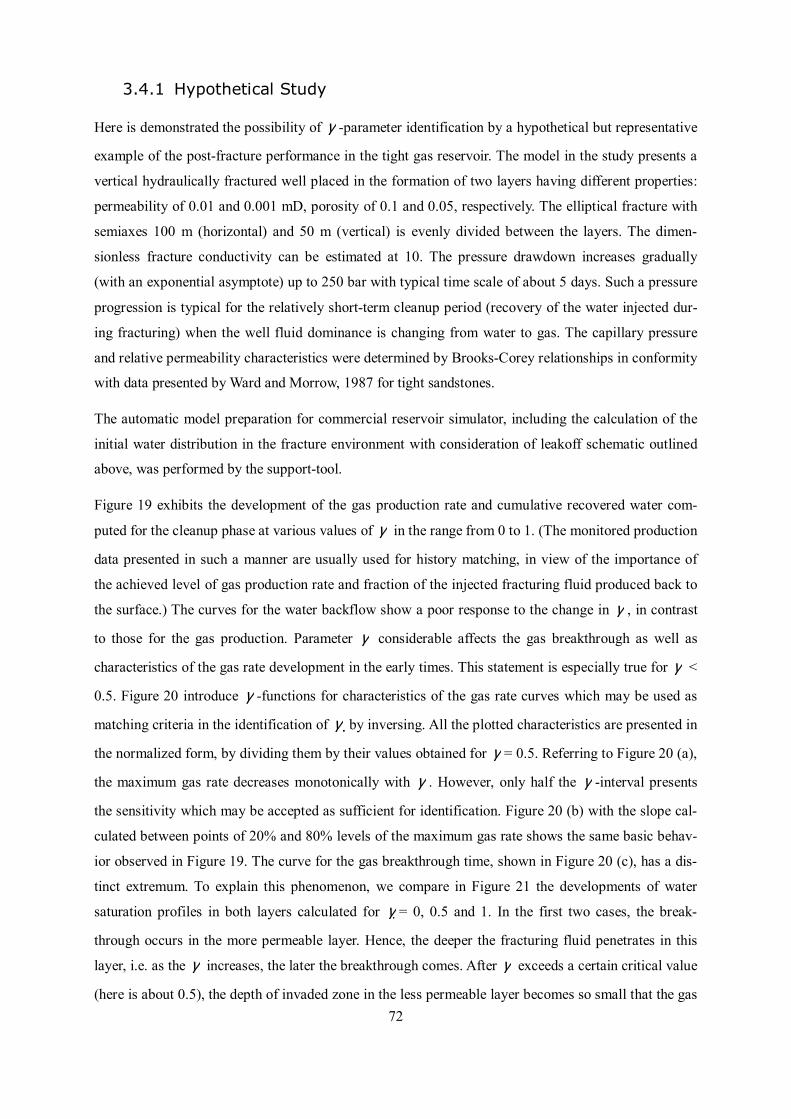
72

3.4.1 Hypothetical Study

Here is demonstrated the possibility of γ -parameter identification by a hypothetical but representative

example of the post-fracture performance in the tight gas reservoir. The model in the study presents a

vertical hydraulically fractured well placed in the formation of two layers having different properties:

permeability of 0.01 and 0.001 mD, porosity of 0.1 and 0.05, respectively. The elliptical fracture with

semiaxes 100 m (horizontal) and 50 m (vertical) is evenly divided between the layers. The dimen-

sionless fracture conductivity can be estimated at 10. The pressure drawdown increases gradually

(with an exponential asymptote) up to 250 bar with typical time scale of about 5 days. Such a pressure

progression is typical for the relatively short-term cleanup period (recovery of the water injected dur-

ing fracturing) when the well fluid dominance is changing from water to gas. The capillary pressure

and relative permeability characteristics were determined by Brooks-Corey relationships in conformity

with data presented by Ward and Morrow, 1987 for tight sandstones.

The automatic model preparation for commercial reservoir simulator, including the calculation of the

initial water distribution in the fracture environment with consideration of leakoff schematic outlined

above, was performed by the support-tool.

Figure 19 exhibits the development of the gas production rate and cumulative recovered water com-

puted for the cleanup phase at various values of γ in the range from 0 to 1. (The monitored production

data presented in such a manner are usually used for history matching, in view of the importance of

the achieved level of gas production rate and fraction of the injected fracturing fluid produced back to

the surface.) The curves for the water backflow show a poor response to the change in γ , in contrast

to those for the gas production. Parameter γ considerable affects the gas breakthrough as well as

characteristics of the gas rate development in the early times. This statement is especially true for γ <

0.5. Figure 20 introduce γ -functions for characteristics of the gas rate curves which may be used as

matching criteria in the identification of γ by inversing. All the plotted characteristics are presented in

the normalized form, by dividing them by their values obtained for γ = 0.5. Referring to Figure 20 (a),

the maximum gas rate decreases monotonically with γ . However, only half the γ -interval presents

the sensitivity which may be accepted as sufficient for identification. Figure 20 (b) with the slope cal-

culated between points of 20% and 80% levels of the maximum gas rate shows the same basic behav-

ior observed in Figure 19. The curve for the gas breakthrough time, shown in Figure 20 (c), has a dis-

tinct extremum. To explain this phenomenon, we compare in Figure 21 the developments of water

saturation profiles in both layers calculated for γ = 0, 0.5 and 1. In the first two cases, the break-

through occurs in the more permeable layer. Hence, the deeper the fracturing fluid penetrates in this

layer, i.e. as the γ increases, the later the breakthrough comes. After γ exceeds a certain critical value

(here is about 0.5), the depth of invaded zone in the less permeable layer becomes so small that the gas

73

forces its way up to the fracture first in this layer. That reverses the trend of the γ -dependence of the

gas breakthrough time, making it unreliable for history matching. Here is the proper point to mention

that the deviation of γ from 0.5 in the direction of its decreasing is much more realistic than in the

opposite direction. This is because the above-named reasons for such a deviation reduce the role of the

formation permeability in controlling the fluid loss processes, rather than the reverse. Thus, γ can be

searched in the range with a higher sensitivity.

0

10000

20000

30000

40000

50000

60000

0 2 4 6 8 10 12Time, days

Gas

pro

duct

ion

rate

, m³/d

ay

0

100

200

300

400

500

600

Cum

ulat

ive

wat

er re

cove

ry, m

³

γ = 0γ = 0.25γ = 0.5γ = 0.75γ = 1______Ρειηε7Ρειηε8Ρειηε9Ρειηε10

Gas

Water

Figure 19: Simulated gas production rate and cumulative water recovery

74

0,8

0,9

1

1,1

1,2

1,3

0 0,2 0,4 0,6 0,8 1γ

Nor

mal

ized

max

imum

gas

rate

(a)

0

0,5

1

1,5

2

2,5

0 0,2 0,4 0,6 0,8 1γ

Nor

mal

ized

gas

rate

slo

pe

(b)

0

0,2

0,4

0,6

0,8

1

0 0,2 0,4 0,6 0,8 1γ

Nor

mal

ized

gas

bre

akth

roug

h tim

e

(c)

Figure 20: Dependence on various parameters on the coefficient (a) Normalised maximum gas rate

(b) Normalised gas rate slope (c) Normalised gas breakthrough

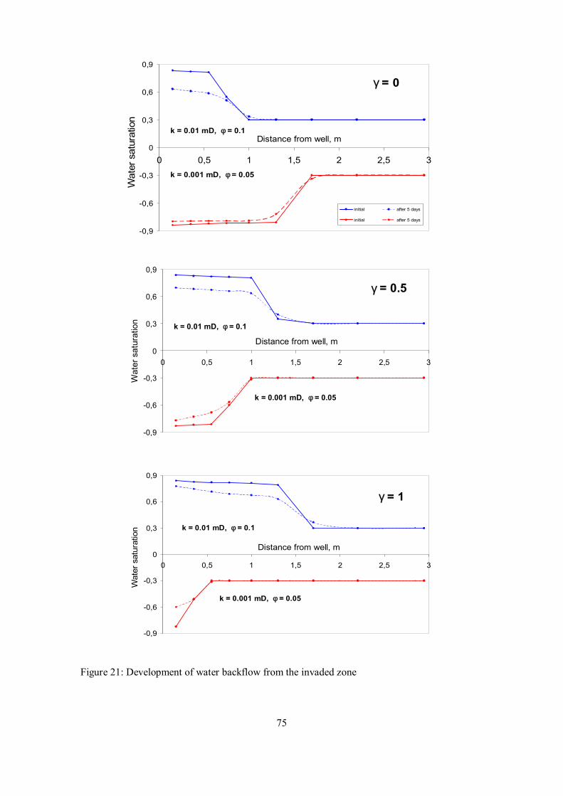
75

-0,9

-0,6

-0,3

0

0,3

0,6

0,9

0 0,5 1 1,5 2 2,5 3

Distance from well, mW

ater

sat

urat

ion

initial after 5 days

initial after 5 days

k = 0.001 mD, φ = 0.05

k = 0.01 mD, φ = 0.1

γ = 0

-0,9

-0,6

-0,3

0

0,3

0,6

0,9

0 0,5 1 1,5 2 2,5 3

Distance from well, m

Wat

er s

atur

atio

n k = 0.01 mD, φ = 0.1

k = 0.001 mD, φ = 0.05

γ = 0.5

-0,9

-0,6

-0,3

0

0,3

0,6

0,9

0 0,5 1 1,5 2 2,5 3

Distance from well, m

Wat

er s

atur

atio

n

γ = 1

k = 0.01 mD, φ = 0.1

k = 0.001 mD, φ = 0.05

Figure 21: Development of water backflow from the invaded zone

76

3.4.2 Case Study

Here, we extend the above concept to the real field case study hydraulically fractured well within the

tight gas formation in North Germany described in the previous chapter 3.3. The fracture is character-

ized by a half-length of 80 m, maximum size in vertical direction of 110 m (net to gross thickness ratio

γ = 0.4), and dimensionless conductivity of about 100. Amount of water injected in the fracture treat-

ment is 300 m³. During cleanup period of 4 days, the pressure drawdown increases up to approxi-

mately 500 bar. A distinctive feature of such a real case is the uncertainty in the two-phase properties

of formation in the fracture vicinity. We introduce the concept of effective relations for the capillary

pressure and relative permeabilities for the heterogeneous system and consider them as a subject of

investigation by history matching, as well as the exponent γ .

As before, in the hypothetical example, the model to simulate the post-fracture performance with res-

ervoir simulator was prepared by the in-house tool. In doing so, it was assumed that the fracture itself

as well as the fracture zones forming the basis of pattern for a piecewise constant proppant (corre-

spondingly, permeability and porosity) distribution is of elliptical form.

Figure 22 demonstrates the best matches between the measured and computed gas and water produc-

tion data which were achieved at fixed γ = 0 and 0.5. The corresponding inverse solutions for relative

permeabilities are plotted in Figure 23. In consequence of a large pressure drawdown, the fitting was

not sensitive to the capillary pressure. One result observed here is that the matched functions of water

relative permeability are not dependent on γ . Also, the optimal curves of cumulative water recovery

are practically the same. Thus, this type of data can not be used for γ -identification.

In contrast, the matched curves for gas relative permeability differ noticeably. Though the correspond-

ing simulated gas rate production graphs agree very closely for much of cleanup period, they do ex-

hibit differences in the gas breakthrough point and slope in the adjacent region. Unfortunately, in this

available example, the indicated distinctions are not significant and there is lack of data monitored in

the transition period. This excludes the possibility of extracting to some extent reliable exponent γ for

leakoff calculation. At the same time, the availability of the relationship for gas relative permeability

opens the way for estimation of the parameter γ on the basis of production data during cleanup. The

sensitivity of these data to γ is confirmed by Figure 24, which shows a considerable deviation from

the curves matched for 5.0=γ when changing γ to 0 and maintaining the relative permeabilities. The

behaviour of the dash curve, which is a solution with 0.1=γ , is consistent with conclusions inferred

from the hypothetical example.

77

0

15000

30000

45000

60000

75000

0 1 2 3 4Cleanup time, day

Gas

pro

duct

ion

rate

, m³/d

ay

0

50

100

150

200

250

Cum

ulat

ive

wat

er re

cove

ry, m

³

Observed gas rate Simulated gas rate, gamma=0,5Simulated gas rate, gamma=0 Observed water recoverySimulated water recovery, gamma=0,5 Simulated water recovery, gamma=0 Simulated gas rate, γ=0Simulated water recovery, γ=0.5

Simulated gas rate, γ=0.5

Simulated water recovery, γ=0

Figure 22: Development of gas flow rate and water recovery at the bottom-hole during the cleanup

period

0

0,05

0,1

0,15

0,2

0,25

0,3

0,35

0,3 0,4 0,5 0,6 0,7 0,8Water saturation

Rel

ativ

e pe

rmea

bilit

y

γ=0.5 γ=0

γ=0.5 γ=0

Gas

Water

Figure 23: Permeability curves matched in the case study at fixed γ =0 and 0.5

78

0

15000

30000

45000

60000

75000

0 1 2 3 4Cleanup time, day

Gas

pro

duct

ion

rate

, m³/d

ay

0

50

100

150

200

250

Cum

ulat

ive

wat

er re

cove

ry, m

³

Observed gas rate Simulated gas rate, gamma=1Simulated gas rate, gamma=0,5 Simulated gas rate, gamma=0Observed water recovery Simulated water recovery, gamma=1 Simulated water recovery, gamma=0,5 Simulated water recovery, gamma=0

Simulated gas rate, γ=1Simulated gas rate, γ=0Simulated water recovery, γ=1Simulated water recovery, γ=0

Simulated gas rate, γ=0.5

Simulated water recovery, γ=0.5

Figure 24: Comparison of production data simulated by the fixed relative permabilities for different

γ -exponents

79

3.5 Automatic Methods of Optimizing of Fractured Wells

The availability of the support tool for integration of the hydraulically fractured well and the fracture

environment into the reservoir simulation model allows not only the identification of main factors

affecting the post-fracture production behaviour of the wellbore but also gives the opportunity to de-

velop the concept for production optimization purposes.

The following chapter illustrates the functioning of that automatic inverse system for optimizing the

gas production from the fractured well. A representative synthetic example was prepared.

For the Calculations the commonly used economic criterion was introduced:

NBDFQ

ANPVi

jgi *

)1(* −

+∆

= ∑ (3.21)

Where:

NPV Net present value,

i Number of production time cycle,

A Coefficient for gas production (related to the gas price),

giQ∆ Well gas production in the i-th time interval,

DF Discount rate,

J Days since start to date / 365,

N Number of fractures,

B Coefficient related to the costs of one fracture.

In view of maximizing of the NPV, the treatment design should be optimized under consideration of its

influence on the fracture conductivity and extension.

The reservoir model with a horizontal fractured well is considered. Three fractures are uniformly lo-

cated along the horizontal well section of about 800 m. All the fractures are assumed to be of the same

geometrical and hydraulic parameter, which are dependent on the fracture treatment design.

Figure 25 serves to obtain the costs needed to increase the fracture conductivity by improvement of the

fracture fluid and proppant parameters without changing the injected slurry volume. The costs of the

treatment refp0 to produce the fracture with a given conductivity refCDF 0, and fixed slurry volume refV

is considered as a scale for dimensionless costs ref

refrefD P

PP0

= which is plotted versus conductivity

80

refCF . The upper index ref means that the curve in Figure 25 is the reference relationship for the cal-

culations with varying slurry volumes. The availability of such a curve implies unique function of

price on the conductivity )( refC

refD FfP = .

Figure 25: Normalized costs of the fracture treatment versus fracture conductivity at the fixed

slurry volume

In its turn, each value of the reference conductivity should be associated with concrete combination of

fracture fluid/proppant. Thus, the choosing the best fracture fluid and proppant parameter means esti-

mation an optimal value of the reference fracture conductivity.

In this synthetic example we considered two parameters to be estimated: reference fracture conductiv-

ity (fracture fluid/proppant system) and injected slurry volume. Thereby it is taken that cost varies in

direct proportion with the injected volume, i.e.:

α⋅== refD

refD P

PPP (3.22)

where,

refVV=α (3.23)

81

At the same time, the change of the injected slurry volume results in the change of the fracture con-

ductivity which is the product of proppant permeability by the propped fracture width. From the rea-

sonable assumption that the fracture grows proportionally in all directions (it was already introduced

in derivation of fracture propagation model (chapter 3.2.3), for the same fluid/proppant system, it fol-

lows:

3/1α⋅= refCC FF (3.24)

For the case with zonal distribution of the fracture parameters, FC refers to the conductivity of the first

elliptical zone, whereby the conductivity ratio between different zones is kept constant. Summarizing,

Equations (3.22, 3.23 and 3.24) the fracture treatment costs PD and the fracture conductivity can be

updated for each set of parameters α and refCF . The influence of the injected slurry volume on the

fracture plane geometry (fracture half-length and height) will be taken into account automatically

when solving the fracture propagation model by the support tool (together with adjustment of fluid

leakoff coefficient).

To demonstrate the optimization algorithm, a short post-fracture production period of 10 days was

taken. The initial value of injected volume V0=300 m³ was the reference value Vref (i.e. 0α =1). The

initial value refCF = 0.1 mD.m is depicted in Figure 25 as a reference point for scaling the costs of the

treatment. The discount factor of 0.15 was applied in Figure 25 for calculation of the net present value.

Figure 26 illustrates the results of the iteratively search procedure in forms of variation the estimated

parameters in conjunction with the development of net present value. Both parameters as well as the

objective function are scaled by their final (optimal) values. Six Levenberg- Marquardt iterations were

required to arrive at the optimum. The total number of performed simulation runs was 19. During the

optimization procedure, the objective value was increased by one third of its initial quantity. This ex-

treme value determines the most cost-effective fracture design, which corresponds to injected fluid

/proppant combination with reference fracture conductivity = 0.08 mD.m and injected slurry volume

α = 3.

For the purpose of clear understanding the inverse technique, the objective-function surface was pro-

duced Figure 27 This procedure implied the approximately hundred additional simulation runs with

different parameter sets in the range near the optimum. The contours on the surface present the isolines

of constant objective function. The similar presentation is shown by the 2D contour graphs Figure 28.

In addition, the scenario of the iterative procedure is depicted by a search trace.

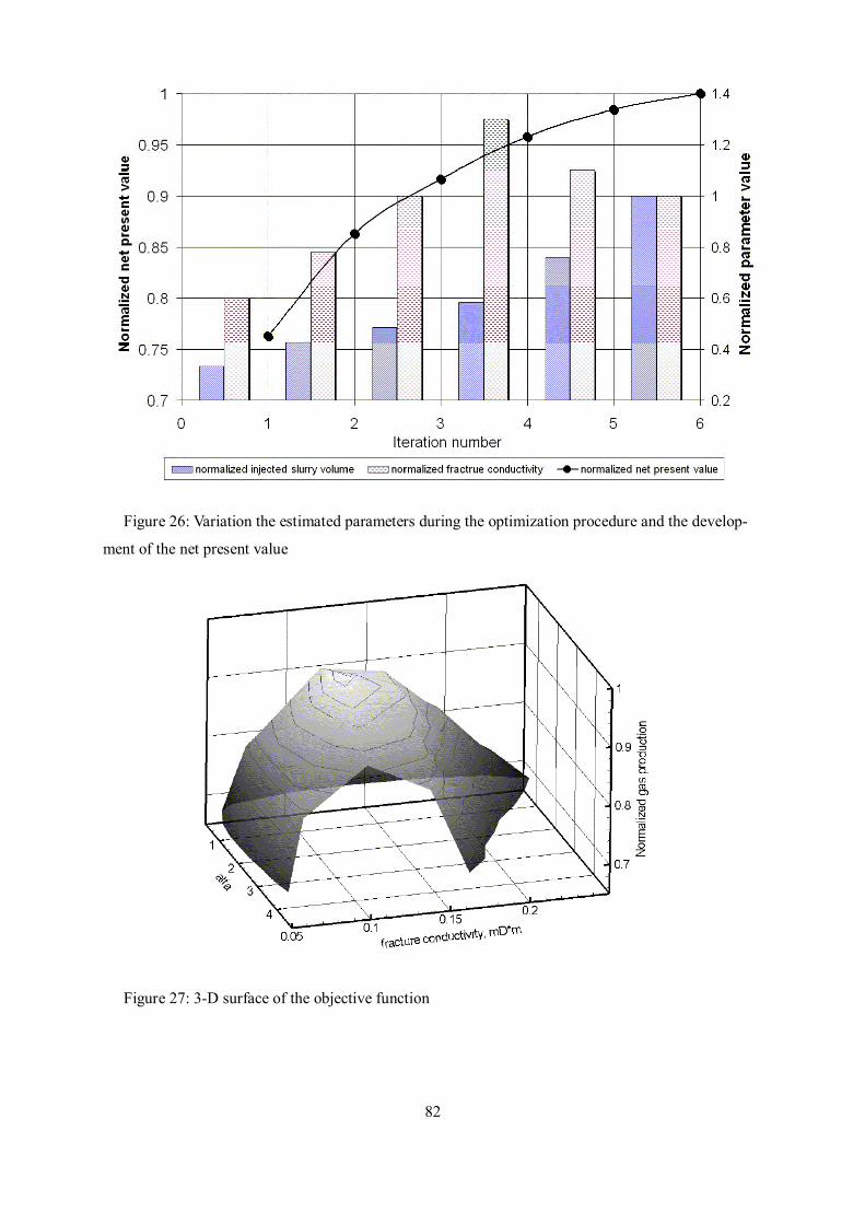
82

Figure 26: Variation the estimated parameters during the optimization procedure and the develop-

ment of the net present value

Figure 27: 3-D surface of the objective function

83

Figure 28: Objective function contour graphs

84

4 Simulation of Inflow whilest Underbalanced Drilling

(UBD) with Automatic identification of Formation

Parameters and Assessment of Uncertainty

In recent years, UBD has become a popular technology. Originally utilized to prevent drilling prob-

lems, its value on the reservoir engineering aspects is more and more recognized. Benefit of UBD

includes the reduction of formation damage by minimizing the drilling fluid leakoff and fines migra-

tion into the formation. Especially in tight formation the invaded drilling fluid can causes the signifi-

cant reduction of gas production do to the water blocking because of two-phase flow and capillary end

effects. At the same time UBD facilitates the possibility for reservoir characterization during drilling.

The purpose of this chapter is to present (i) how to use the inflow data for the evaluation of formation

properties and (ii) how to cope with the uncertainty of the results.

Since the wellbore pressure is lower than the one in the reservoir, there is a permanent inflow of reser-

voir fluids during the underbalanced operation UBO (and, possibly, an outflow of drilling mud due to

countercurrent imbibition). The inflow rates can be obtained by balancing injected and produced flu-

ids. In-situ downhole conditions like temperature and flowing wellbore pressure are usually continu-

ously measured while drilling. Applying inverse modeling methods, it is now possible to determine

reservoir parameters such as permeabilities and pore pressures by extracting the productivity signature

of the reservoir out of the production data. Although the short drilling periods only give insight into

the nearer wellbore vicinity, valuable information about the reservoir can be obtained in this way. Pro-

ductive reservoir zones and formation properties can be determined provided there is a proper flow

monitoring at the surface. This offers significant benefits in both the production optimization and res-

ervoir characterization but also in the justification of UBD.

In this chapter is demonstrated the usage of a reservoir simulation tool, coupled with a parameter iden-

tification method for the purpose of automated reservoir characterization during the drilling. In par-

ticular, the tasks from the reservoir engineering perspective, tracked here, are:

• Detection of the layering,

• Identification of layer permeabilities (or other layer properties) and, optionally,

• Assessment of the reservoir formation damage.

Using statistical methods, it is not only possible to obtain important reservoir parameters but also to

assign the corresponding uncertainties. In the modeling workflow, those can be useful for the valida-

tion of the reservoir model with the prior geological model (Figure 29).

85

The workflow of the UBD reservoir characterization tool enables also “simulation while drilling”. Its

usage is hence not limited to the common post drilling evaluation but also facilitates control/decide

mechanisms in terms of optimal control during the drilling process.

Figure 29: Components for UBD

4.1 Literature review

An early discussion of reservoir characterization during drilling can be found in Kardolus und van

Kruijsdijk, 1997, van Kruijsdijk and Cox, 1999 and Larsen and Nilsen 1999. The authors adopted con-

stant pressure-type analytical solutions to account for a constant underbalanced pressure and the ongo-

ing penetration during the drilling process to identify permeabilities in layered reservoirs (with a pre-

defined layering) for vertical and horizontal wells. Flow was considered solely one-dimensional (i.e.

radial). Since using analytical models, nonlinearities such as multiphase flow were not taken into ac-

count. Only reservoir flow was part of the UBD-loop.

Hunt and Rester, 2000 presented a solution of the diffusivity equation representing the reservoir re-

sponse during UBD, by including the time dependency of the boundary condition at the wellbore. As

drilling progresses, the length of the wellbore increases and the fluid flow rate from the reservoir

changed in response to the well length and wellbore conditions.

Kneissl, 2001 presented a methodology allowing derivation of reservoir characteristics in real time

while drilling underbalanced. The analysis was based on transient pressure-test interpretation, leading

to a locally performed multi-rate well test, conducted without any interruption to the drilling process,

or any zonal isolation within the wellbore.

Vefring et al. 2002 discussed the coupling of transient wellbore to transient reservoir for the purpose of

estimating near-well reservoir properties. The reservoir model was calibrated using only the well in-

flow data usually measured during UBD. Parameters were the permeability and reservoir pressure for

86

n predefined zones. As estimation techniques, the least square methodology as well as the ensemble

Kalman filter was implemented. As in all of the previously mentioned works, the main restriction in

their model was the using of a transient analytical model for describing the reservoir fluid which is not

capable of capturing formation damage during drilling.

Biswas et al. 2003 presented a sophisticated UBD reservoir characterisation tool. For the first time, a

discrete reservoir simulation model was coupled with a discrete wellbore flow model to consider the

flow during UBD from the reservoir up to the surface where fluid measurements are taken. The reser-

voir tool was a two-phase, two dimensional Finite Element simulator, which was intrinsically based on

unstructured grids. The commercial transient mechanistic multiphase wellbore flow model captured

two-phase flow. A genetic algorithm approach, coupled with a one-dimensional search scheme was

applied to derive reservoir parameters. Determination of the layering, however, was not included in

their model as well as a statistical analysis.

4.2 Simulation of Reservoir Flow during UBD

For the simulation of the formation fluid flow during UBD there are two main issues, which need to be

considered with care simulating reservoir fluid flow during UBD, in particular, when dealing with

formation hydraulically damage processes.

(1) Boundary conditions.

Setting the appropriate boundary conditions is a crucial factor for hydrodynamic simulation of UBD.

The pressure in the well is controlled and monitored during the drilling process in the field. Further-

more, the drilling fluid within the drilling interval needs to be taken into account. That is important

since countercurrent imbibition of the drilling fluid into the formation can cause formation damage

despite the gas influx into the well. To get a proper depiction of the drilling process, both the known

drilling pressure and the saturation conditions need to be applied in the numerical reservoir model. The

lack of such a well control mode in commercial simulators is a main reason for the variety of simplifi-

cations assumed so far in previous studies.

(2) Discretisation.

Conventional Cartesian grids with the common grid block sizes are generally not suitable to track near

wellbore phenomena occurring during UBD. To capture the radial flow around a wellbore up to well

test accuracy, the nearer well vicinity needs a high level of grid refinement with grids honouring the

flow pattern and the pressure gradients. However, to integrate both timescales with the early time tran-

sients around the wellbore and the full field characteristics with the late time response, a hybrid grid is

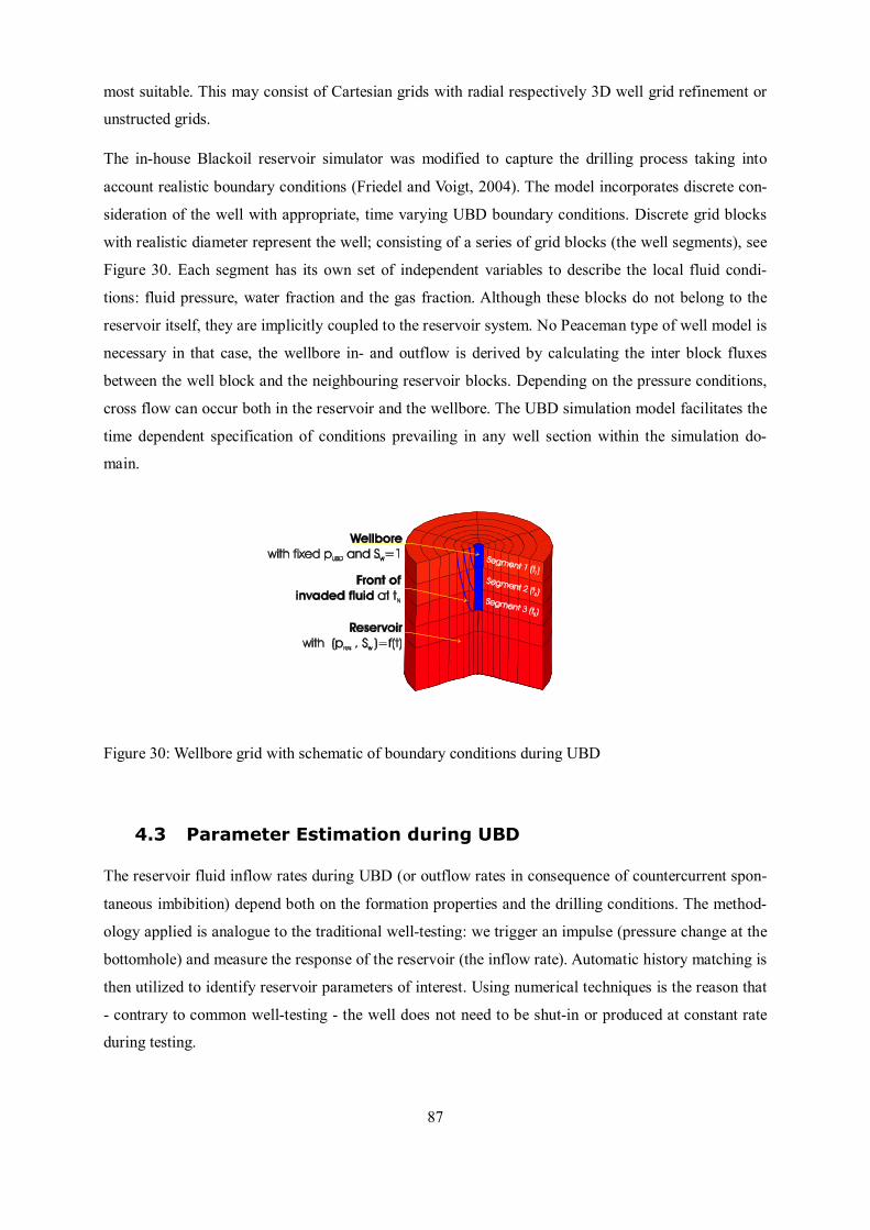
87

most suitable. This may consist of Cartesian grids with radial respectively 3D well grid refinement or

unstructed grids.

The in-house Blackoil reservoir simulator was modified to capture the drilling process taking into

account realistic boundary conditions (Friedel and Voigt, 2004). The model incorporates discrete con-

sideration of the well with appropriate, time varying UBD boundary conditions. Discrete grid blocks

with realistic diameter represent the well; consisting of a series of grid blocks (the well segments), see

Figure 30. Each segment has its own set of independent variables to describe the local fluid condi-

tions: fluid pressure, water fraction and the gas fraction. Although these blocks do not belong to the

reservoir itself, they are implicitly coupled to the reservoir system. No Peaceman type of well model is

necessary in that case, the wellbore in- and outflow is derived by calculating the inter block fluxes

between the well block and the neighbouring reservoir blocks. Depending on the pressure conditions,

cross flow can occur both in the reservoir and the wellbore. The UBD simulation model facilitates the

time dependent specification of conditions prevailing in any well section within the simulation do-

main.

Figure 30: Wellbore grid with schematic of boundary conditions during UBD

4.3 Parameter Estimation during UBD

The reservoir fluid inflow rates during UBD (or outflow rates in consequence of countercurrent spon-

taneous imbibition) depend both on the formation properties and the drilling conditions. The method-

ology applied is analogue to the traditional well-testing: we trigger an impulse (pressure change at the

bottomhole) and measure the response of the reservoir (the inflow rate). Automatic history matching is

then utilized to identify reservoir parameters of interest. Using numerical techniques is the reason that

- contrary to common well-testing - the well does not need to be shut-in or produced at constant rate

during testing.

88

The general idea, pursued here, is simple: we start with a simple reservoir model (consisting of one

layer which is penetrated at that point of time) and extend and update it steadily throughout the drilling

when more production data from the reservoir is accumulated. As the drilling proceeds and the number

of available production data increases, sequential history match procedure gives the possibility for

estimating the layering structure of the penetrated reservoir. Based on a statistical analysis of the in-

verse problem we identify the optimal level of parameterization as the quality and quantity of meas-

ured data allows for. For the history match procedure an in-house optimization-toolbox based on the

Gauss-Newton gradient method is used. The UBD simulator controls the tool and is tightly coupled to

the optimizer. It is performed automatically and includes a continuous updating of the reservoir simu-

lation model.

4.4 Identification Procedure

The basic procedure consists of the following steps:

(1) Initially, we start with a drilling profile consisting of one homogeneous region. There is no pre-

defined layering (the simulation model consist only of one layer). Furthermore, we specify a time in-

terval for testing the mismatch between measured and simulated rates. This time or length interval for

testing the Objective Function (OF) is basically a detection frequency and is related to the penetration

rate. It depends on the quality of the measured data as well as on CPU time constraints. Its size, e.g., 2

meters, will later be the minimum thickness for any layer in the final reservoir model.

(2) Then, the UBD-process is simulated for the first detection interval, taking into account the given

rate of penetration. The gas inflow rate is derived by gradually imposing the observed UBD pressure

to the corresponding well segment.

(3) Using the available inflow data, the optimization code estimates the permeability value. The

reservoir model is updated accordingly.

(4) As the drilling proceeds, the UBD simulator proceeds to the next time point tn introducing the

next well segment under stated reservoir model and compares the simulated with the observed produc-

tion data. Based on statistical analyses, the discrepancy between the observed and simulated inflow

helps to determine the new level of parameterization. To decide about the new degree of freedom, we

use the following consideration:

Since the observed data can be regarded as random variables (because of measurement errors), the

calculated value of the mismatch or objective function (OF) until time nt can be assumed −2χ dis-

tributed with (Nm - Np) degrees of freedom. This implies that

89

( ) pm NNOFE −= (4.1)

( ) ( )pm NNOF −= 2σ (4.2)

Nm is the number of measured values till nt , Np is the number of identified parameters, E denotes the

statistical expectation and σ the standard deviation.

(5) At this point of time, the indicator for further parameterization is expressed as follows:

If

( ) ( )pmpm

N

i i

obsi

calci NNNNTOL

uum

−+−=>−∑

=2

12

2

σ (4.3)

then the new parameter (as the discontinuity of the permeability layering) is introduced at this time

step. Or with other words, until the posteriori error variance, expressed with following equation:

( )pm

N

i

obsi

calci

NN

uus

m

−

−=∑

=1

2

20 (4.4)

is consistent with the assumption about the measurement error, the underlying parameterized model is

accepted to satisfy the “modeller’s expectation” on the observed system, the permeability layering

structure will be kept constant and the process can be continued from step (3). If the estimated error

variance is significantly larger than or the above condition (Equation 4.3) is fulfilled, then there is a

need to improve the mismatch between the observed and calculated responses. That comes along with

the necessity of adding a new parameter. Thus, we can identify the boundary of a reservoir layer. After

this, at the given refinement level, the parameter estimation process will be continued from point (2)

until the end of the UBD interval is reached.

The automated workflow of the identification procedure is shown in Figure 31.

In the course of steps (1)-(4), the user can decide if, at given drilling time tn, only the parameters of

the corresponding layer or segment are determined or if the parameters of the previous segments

should be included. That is usually not necessary and numerically expensive. However, it can be use-

ful, e.g., to detect lateral unconformities. As obvious, the parameter estimation problem is solved

through successive approximations by identifying the layering structure at which the permeabilities are

described. The process is stopped when the parameterization level is consistent with the assumptions

about the measurement “precision”. The parameterization techniques proposed automatically guards

the model against overparametrization, thus, meets the principle of parsimony. When the data are of

90

relatively poor quality and there is no prior information, it is not justified to use highly detailed mod-

els.

Figure 31: UBD Coupling

4.5 Uncertainty Analyses

Since the measured production data is regarded as random variable, the actually observed inflow pro-

file is always tainted with uncertainties. The statistical analysis of the estimated parameters obtained

by using observed data is hence one prime objective of the reservoir characterization process. Based

on the nonlinear regression method, valuable statistics can be generated for the determined model pa-

rameters k*h for all identified reservoir layers. Under the assumption of linearity and normality, the

joint probability distribution of the estimated parameters is fully described by the covariance matrix

(the inverse of the Hessian matrix):

[ ] 120)ˆ( −⋅=Θ HsCov (4.5)

The diagonal elements of matrix )ˆ(ΘCov equal the variances of the estimated parameter values. The

analysis of estimated variance is very useful for calculating two other statistics: (i) confidence inter-

vals for parameter values (the range that has a stated probability of containing the true value) and (ii)

coefficients of variation (with which the relative accuracy of different parameter estimates can be com-

pared).

As above equation reveals, the estimated covariance matrix, )ˆ(ΘCov , depends both on the goodness

of fit (s0) and the sensitivity of the simulated system behavior to a small parameter change (H). The

relative measure of parameter sensitivity is provided by the composite scaled sensitivity (CSS), which

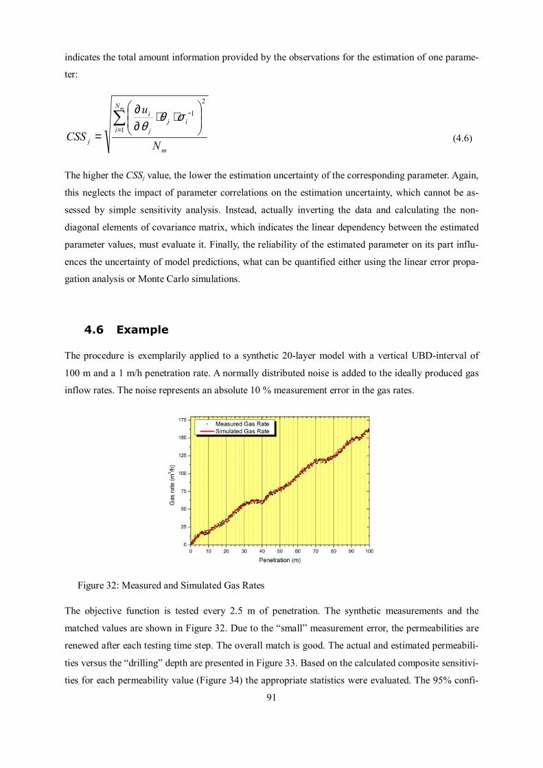
91

indicates the total amount information provided by the observations for the estimation of one parame-

ter:

m

N

iij

j

i

j N

u

CSS

m

∑=

−

⋅⋅

∂∂

=1

2

1σθθ

(4.6)

The higher the CSSj value, the lower the estimation uncertainty of the corresponding parameter. Again,

this neglects the impact of parameter correlations on the estimation uncertainty, which cannot be as-

sessed by simple sensitivity analysis. Instead, actually inverting the data and calculating the non-

diagonal elements of covariance matrix, which indicates the linear dependency between the estimated

parameter values, must evaluate it. Finally, the reliability of the estimated parameter on its part influ-

ences the uncertainty of model predictions, what can be quantified either using the linear error propa-

gation analysis or Monte Carlo simulations.

4.6 Example

The procedure is exemplarily applied to a synthetic 20-layer model with a vertical UBD-interval of

100 m and a 1 m/h penetration rate. A normally distributed noise is added to the ideally produced gas

inflow rates. The noise represents an absolute 10 % measurement error in the gas rates.

Figure 32: Measured and Simulated Gas Rates

The objective function is tested every 2.5 m of penetration. The synthetic measurements and the

matched values are shown in Figure 32. Due to the “small” measurement error, the permeabilities are

renewed after each testing time step. The overall match is good. The actual and estimated permeabili-

ties versus the “drilling” depth are presented in Figure 33. Based on the calculated composite sensitivi-

ties for each permeability value (Figure 34) the appropriate statistics were evaluated. The 95% confi-

92

dence intervals for every identified parameter are included in Figure 33 The analysis of the non-

diagonal elements of the covariance matrix reveals that the correlation coefficient between all parame-

ter pairs in the present case is lower then 0.8. This indicates linear independency between the esti-

mated permeability values. The discrepancy between the estimated and true model is satisfactory and

the main trend is reproduced.

Figure 33 Estimated and true permeability versus drilled depth

Figure 34: Composite Scaled Sensitivities (CSS)

93

4.7 Outlook: Optimization Approach for UBD

The UBD reservoir characterization model is not only applicable for identification of layer properties

but also for optimum control strategies. This is further promoted due to the numerical efficiency of the

workflow model proposed with its technique to gradually extend the model size. Although not accom-

plished yet, the model can thus be used to support the design of the drilling process by “real-time”

simulation of the drilling process (Figure 35).

Potential application is, e.g., the adjustment of drilling parameters such as UBD pressure and penetra-

tion rate to minimize formation damage during drilling. However, in order to get a full description of

the drilling process, the wellbore flow needs to be integrated. Due to the modular structure of the tool

it can be extended in the future.

Figure 35: Control and optimization loop for UBD processes

94

5 Summary

The present thesis focuses on the following issues:

(i) Inverse modeling methods for characterization of tight-gas reservoirs, (ii) the numerical investiga-

tions of advanced well stimulation techniques, concerning hydraulic fracturing as well as underbal-

anced drilling, and (iii) the statistical analyses of results for identification of the optimal level of

parameterization for calibrated model as quality and quantity of the measured data justifies.

The automatic model calibration is formulated as an optimization problem, which has to be solved in

the presence of uncertainty because the available observed field data cannot be identical to the system

responses calculated with a reservoir model due to the measurement errors and the simplified nature of

the numerical model (model structure error).Because of the complexity of many real systems under

study the number of reservoir parameters is usually larger than the available data set, therefore the

solution is non-unique and the inverse problem is ill-posed. While adding features to a model is often

desirable to minimize the misfit function between simulated and observed values, the increased com-

plexity comes with a cost. In general, the more parameters contained in a model, the more uncertain

are parameter estimates. Often it is advisable to simplify some representation of reality in order to

achieve an understanding of the dominant aspects of the system under study. The study of the inverse

problems in the stochastic framework provides capabilities using diagnostic statistics to quantify a

quality of calibration and the inferential statistics that quantify reliability of parameter estimates and

predictions. The statistical criteria for model selection may help the modelers to determine an appro-

priate level of complexity of parameterization and one would like to have as good an approximation of

the structure of the system as the information permits.

In the present thesis, the statistical model selection approach, based on the Kullback-Leibler informa-

tion, was used to choose the best parameter zonation pattern for a reservoir model. It measures directly

the model departure from the true system, taking into account the bias and variance between the pre-

dicted and observed system responses. This approach balances the trade-off between increased infor-

mation and decreased reliability, which is fundamental to the principle of parsimony. In the case where

no single model is clearly superior to some of the others, it is reasonable to use the concepts for model

averaging for translating the uncertainty associated with model selection into the uncertainty to assess

the model prediction performance.

In this thesis the inverse modeling techniques was applied for characterization of tight-gas reservoirs

and in this context the numerical investigation of the production behavior of the hydraulically frac-

tured wells was an essential part of the investigations. The objective was the identification and analy-

ses of the main damage mechanisms influencing the low productiveness of the fractured wells using

the history match procedure of field data from a German tight gas reservoir.

95

To simplify the workflow of hydraulic fractured well simulation by automatically setting up an appro-

priate reservoir model, an in-house support tool was used, which provides the coupling of commercial

fracturing software with reservoir simulator ECLIPSE. The stationary fracture geometry, the distribu-

tion of the hydraulic parameters within the fracture, as well as fluid distribution in the damage zone

were main subjects of modeling process. The problem of the model initialization with respect to the

fluid saturation had received a special attention. By the approach, based on the simplified fracture

propagation model, the fracturing treatment scenario was translated into the spatial distribution of the

exposure time of the fracturing fluid to the formation. The leakoff coefficient was iteratively adjusted

in the course of solving this model and was regarded as a function of the permeability and net thick-

ness ratio. The reconstructed data on the exposure time and leakoff coefficient were used to calculate

the saturation profiles adjacent to the fracture surface. Thus, the approach involves the reasonably

adequate consideration of the prehistory of the fracture.

Thus, the tool is well suited for model calibration purposes and enables the accurate simulation of the

early cleanup period as well as the long-term behavior of the fractured wells. Based upon the results of

the numerical simulations of the production behavior of fractured well within a Rotliegend Tight Gas

formation in North Germany the following conclusions were offered: (i) the history matching of

cleanup- und long-term production behavior of a fractured wells can be realized with consideration of

mechanical and hydraulical damages in the fracture environment as well as with the matching parame-

ter of relative gas permeability. (ii) matching the cleanup period without consideration of a mechanical

damage zone leads to untypical relative permeability function for gas. Additionally it failed to predict

the long-term production period; (iii) cumulative water recovery, gas breakthrough time and gas rate

can be considered representative matching criteria in tight gas formations.

In the present thesis is presented the possibility for reservoir characterization and automatic identifica-

tion of formation parameters during Underbalanced Drilling. For these purposes a UBD reservoir

simulation tool is coupled with gradient-based Gauss-Newton optimization routines, stepping towards

an integrated UBD reservoir characterization system. The UBD reservoir simulator which provides an

accurate depiction of the physical processes during UBD, taking into account the boundary conditions

at the wellbore, was coupled to a parameter estimation tool that allows for identification of reservoir

heterogeneity, in particular the layering with the corresponding permeabilities such that the over-

parameterization is avoided. Simultaneously, an extensive statistical analysis is conducted which en-

ables an evaluation of the uncertainty of the estimated parameters. The framework is fully automated

and can be utilized for real-time history matching during UBD. Derivation of the pore pressure and

permeability profiles of the reservoir while drilling furthermore potentially dispenses with the cost and

emissions associated to post drill well testing, allows determination of long term well productivity real

time, and could give vital early warning of high pressure zones in the reservoir, critical kick-avoidance

information. The main advantages of the methodology proposed are its ability to detect reservoir

96

boundaries (up to a minimal resolution according the detection frequency) and its numerical efficiency

by gradually improving and enlarging the reservoir model.

97

Bibliography

/1/ Akaike, H., Information Theory and an Extension of the Maximum Likelihood Principle (Proc.

2nd International Symposium on Information Theory). Akademia Kiad, Budapest. 267-281. 1973.

/2/ Akaike, H., On the Likelihood of a Time Series Model. (The Statistician), Vol. 27, 217-235.

1978.

/3/ Banerjee, R., Gunasekera, D., and Fletcher, C.K.J.: Simulation of Hydraulically Fractured Hori-

zontal and Vertical Wells to Well Testing Accuracy Using Unstructured Grids, proceedings of the 7th

European Conference on the Mathematics of Oil Recovery, Baverno, Italy (2000), M-21.

/4/ Basquet, R., Alabert, F., Caltagirone, J-P., Analytical Solutions for Productivity Evaluation of

Multifractured Wells in Multilayered and Bounded Reservoirs, SPE 56683, SPE Annual Technical

Conference and Exhibition, 3-6 October 1999, Houston, Texas.

/5/ Bastian, P.A. and Sherman, J.B.: Analysis of a Hydraulically Fractured, Low-Permeability Gas

Reservoir Using Numerical Simulation, SPE 21511, proceedings of the SPE Gas Technology Sympo-

sium, Houston, Texas (1991), 172-181.

/6/ Behr, A., Mtchedlishvili G.: “Leakoff Modeling of Fluid Injected in Gas Reservoir at Fracture

Stimulation” prepared for Underground Injection Science and Technology Conference 2003, Berkeley,

California, USA

/7/ Behr, A.; Mtchedlishvili, G.; Friedel, T.; Häfner, F.: Initialization of Reservoir Model with Hy-

draulically Fractured Well for Simulation of Post-Fracture Performance, SPE 82298, prepared for the

European Formation Damage Conference 2003, The Hague, 13-14 May (2003).

/8/ Bennett, C.O., Reynolds, A.C., Raghavan, R., Elbel, J.L., Performance of Finite-Conductivity,

Vertically Fractured Wells in single-Layers Reservoirs, SPE 11029, SPE Formation Evaluation, Au-

gust, 1986, pp. 399-420.

/9/ Bennion, D. B.; Thomas, F. B.; Ma T.: Formation Damage Processes Reducing Productivity of

Low Permeability Gas Reservoirs. (SPE-Paper 60325), 2000. presented at the SPE Rocky Mountain

Regional/Low Permeability Reservoirs Symposium and Exhibition held in Denver, Colorado.

/10/ Bissell, R.C., Calculating optimal parameters for history matching, 4th European Conference on

the Mathematics of Oil Recovery, Roros, Norway June 7-10, 1994.

/11/ Biswas, D., Suryanarayana P.V., Frink P.J., Rahman S.: An Improved Model to Predict Reser-

voir Characteristics During Underbalanced Drilling. (SPE-Paper 84176), 2003. Presented at the SPE

Annual Technical Conference and Exhibition held in Denver, Colorado.

98

/12/ Burnham, K.P., Anderson, D. R., Model Selection and Inference,. Springer-Verlag. 1998

/13/ Byrnes, A. P.; Castle, W.: Comparison of Core Petrophysical Properties Between Low-

Permeability Sandstone Reservoirs: Eastern U. S. Medina Group and Western U. S. Mesaverde Group

and Frontier Formation. (SPE-Paper 60304), 2000.

/14/ Carrera, J., and S. P. Neuman, Estimation of aquifer parameters under transient and steady state

conditions: 1. Maximum likelihood method incorporating prior information, Water Resour. Res.,

22(2), 199–210, 1986a.

/15/ Carrera, J., and S. P. Neuman, Estimation of aquifer parameters under transient and steady state

conditions: 2. Uniqueness, stability, and solution algorithms, Water Resour. Res., 22(2), 211–227,

1986b.

/16/ Carrera, J., and S. P. Neuman, Estimation of aquifer parameters under transient and steady state

conditions: 3. Application to synthetic and field data, Water Resour. Res., 22(2), 228–242, 1986c

/17/ Christie, M., Subbey, S., Sambridge, M., Thiele M., Quantifying Prediction Uncertainty in Res-

ervoir Modelling Using Streamline Simulation, 15th ASCE Engineering Conference, Columbia Uni-

versity, New York, June 2-5, 2002.

/18/ ECLIPSE 100 User Manual, Schlumberger_GeoQuest, Abingdon, 2000.

/19/ Ehrl, E., Schueler, S.K., Simulation of a Tight Gas Reservoir with Horizontal Multifractured

Wells”, SPE 65108, SPE European Petroleum Conference, 24-25 October 2000, Paris, France.

/20/ Floris, F.J.T., Bush, M.D., Cuypers, M., Roggero, F., Syversveen, A-R., Comparision of produc-

tion forecast uncertainty quantification methods – An integrated study, to appear in Petroleum Geo-

science. 2000

/20/ Friedel T, Numerical Simulation of Production from Tight-Gas Reservoirs by Advanced Stimu-

lation Techniques. Dissertation, TU Bergakademie Freiberg,2004

/21/ Friedel, T., Nekrassov, A., Behr, A., Mtchedlishvili, G., and Haefner, F.: Representation of Frac-

tured Well to Numerical Modeling Post-Fracturing Production from Tight Reservoirs, proceedings of

the 8th European Conference on the Mathematics of Oil Recovery, Freiberg, Germany (2002), E36.

/22/ Friedel T. and Voigt H.-D.: Numerical Simulation of the Gas Inflow during Underbalanced

Drilling (UBD) and Investigation of the Impact of UBD on the Longtime Productivity of a Well. (SPE-

Paper 91588), 2004. Presented at the 2004 IADC/SPE UBD Conference & Exhibition, The Wood-

lands, Texas.

/23/ Goldberg, D.E.: Genetic Algorithms in Search, Optimization and machine Learning, Addision-

Wesley, Reading (1989)

99

/24/ Gómez, S., Gosselin O., and Barker, J.W.: Gradient-Based History Matching with a Global Op-

timization Method,” paper SPE 56756, presented at the 1999 SPE Annual Technical Conference and

Exhibition, Houston, Oct. 3-6.

/25/ Haefner et al.: Simulation des Produktionsverhaltens gefracter Bohrungen in geringpermeablen

Gaslagerstätten, Projekt 593-9 des DGMK-Forschungsprogramm 593: „Tight Gas Reservoir-Erdgas

für die Zukunft“, Abschlußbericht, 2002.

/26/ Holditch, S.A.: Factors Affecting Water Blocking and Gas Flow From Hydraulically Fractured

Wells , Journal of Petroleum Technology, Dec. 1979, pp. 1515-1524

/27/ Holland, J.H.: Adaptation in natural and artificial Systems, University of Michigan press, Ann

Arbor, Michigan (1975).

/28/ Howard, G.C. and Fast, C.R.: Hydraulic Fracturing, SPE Monograph. Series, Dallas (1970), Vol.

2.

/29/ Hunt, J.L. and Rester, S.: Reservoir Characterization During Underbalanced Drilling: A New

Model. (SPE-Paper 59743), 2000. Presented at the 2000 SPE/CERI Gas Technology Symposium held

in Calgary, Alberta, Canada.

/30/ Kardolus, C.B. and van Kruijsdijk, C.P.J.W.: Formation Testing While Underbalanced Drilling.

(SPE-Paper 38754), 1997. Presented at the SPE Annual Technical Conference held in San Antonio,

Texas.

/31/ Kashyap, R. L., Optimal choice of AR and MA parts in Autoregressive Moving Average Models

(IEEE Transactions on Pattern Analysis and Machine Intelligence), Vol. 4, 99-104. 1982

/32/ King, P.R., Harding, T.J., and Radcliffe, N.J.: “Optimisation of Production Strategies using

Stochastic Search Methods,” Proc., 5th European Conference on the Mathematics of Oil Recovery

(1996), Leoben, Sept 3-6.

/33/ Kneissl W.: Reservoir Characterization Whilst UnderBalanced Drilling. (SPE-Paper 67690),

2001. Presented at the 2001 SPE/IADC Drilling Conference held in Amsterdam, The Netherlands.

/34/ Larsen L. and Nilsen F.: Inflow Predictions and Testing While Underbalanced Drilling. (SPE-

Paper 56684), 1999. presented at the SPE Annual Technical Conference held in Houston, Texas.

/35/ Liermann N.; Jentsch M.: Tight-Gas-Reservoirs – Erdgas für die Zukunft. Erdöl Erdgas Kohle,

(7/8): 270-273, Jul./Aug. 2003. Presented at the DGMK-Spring meeting 28-29 April 2003 held in

Celle, Germany.

/36/ Nghiem, L.X., Forsyth, P.A., and Behie, A.: A Fully Implicit Hydraulic Fracture Model, JPT,

July (1984), 1191-1198.

100

/37/ Ouenes, A., and Bhagavan, S.: Application of SimulatedAnnealing and Other Global Optimiza-

tion Methods to Reservoir Description: Myths and Realities, paper SPE 28415 presented at the 1994

SPE Annual Technical Conference and Exhibition, New Orleans, Sept. 25-28.

/38/ Ouenes, A., Brefort, B., Meunier, G., and Dupéré, S.: A New Algorithm for Automatic History

Matching: Application of Simulated Annealing Method to Reservoir Inverse Modeling, paper SPE

26297 (1983).

/39/ Penny G. S.; Soliman M. Y.; Conway M.W.; Briscoe J. E.: Enhanced Load Water-Recovery

Technique Improves Stimulation Results. (SPE-Paper 12149), 1983.

/40/ Russo, D.: Determining soil hydraulic properties by parameter estimation: On the selection of a

model for the hydraulic properties, Water Resour. Res., 24(3), 453-459, 1988.

/41/ Russo, D., E. Bresler, U. Shani, and J. C. Parker: Analyses of infiltration events in relation to

determining soil hydraulic properties by inverse problem methodology, Water Resour. Res., 27(6),

1361-1373, 1991.

/42/ Sambridge, M. (1999a). Geophysical Inversion with a Neighbourhood Algorithm I: searching a

parameter space, Geophys. J. Int., 138, 479- 494.

/43/ Schwarz, G., Estimating the dimension of a model (Annals of Statistics), Vol. 6, 461-464. 1978.

/44/ Settari, A.: Partially Decoupled Modeling of Hydraulic Fracturing Process, SPE 16031, pro-

ceedings of the SPE Reservoir Simulation Symposium, San Antonio (1987), 37-44.

/45/ Settari, A.: Simulation of Hydraulic Fracturing Processes, SPEJ, December (1980), 487-500.

/46/ Shaoul J.R., Behr A., Mtshedlishvili G., Developing a Tool for 3D Reservoir Simulation of Hy-

draulically Fractured Wells, IPTC 10182, This paper was prepared for presentation at the International

Petroleum Technology Conference held in Doha, Qatar, 21–23 November 2005.

/47/ Sherman, J. B., Holditch, S.A.: Effect of Injected Fracture Fluids and Operating Procedures on

Ultimate Gas Recovery, SPE 21496, (1991), 163-175.

/48/ Steinberg, D. M., and W. G. Hunter: Experimental design: Review and comment, Technomet-

rics, 28, 71-97, 1984.

/49/ Sun, N.-Z., Inverse Problems in Groundwater Modeling, Kluwer Acad., Norwell, Mass.,1994.

/50/ Tannich, J.D.: Liquid Removal from Hydraulically Fractured Gas Wells, Journal of Petroleum

Technology, Nov. 1975, pp. 1309-1317

101

/51/ van Kruijsdijk, C.P.J.W. and Cox, R.J.W.: Testing While Underbalanced Drilling: Horizontal

Well Permeability Profiles. (SPE-Paper 54717), 1999. Presented at the SPE European Formation

Damage Conference held in The Hague, The Netherlands.

/52/ Vefring, E.H.; Nygaard, G.; Fjelde, K.K.; Lorentzen, G.N.; Naevdal G.; Merlo A.: Reservoir

Characterization During Underbalanced Drilling: Methodology, Accuracy, and Necessary Data. (SPE-

Paper 77530), 2002. Presented at the 2002 Annual Technical Conference and Exhibition held in San

Antonio, Texas.

/53/ Ward, J. S.; Morrow, N. R.: Capillary Pressure and Gas Relative Permeabilities of Low-

Permeability Sandstone. SPEFE, (SPE-Paper 13882), 1987.

/54/ Web site: http://www.nitg.tno.nl/punq/