Inverse Kinematics of a 10 DOF Modular Hyper-Redundant ...

Inverse Kinematics of a 10 DOF ModularHyper-Redundant Robot Resorting toExhaustive and Error-Optimization

Methods:A Comparative Study

Mario Sáenz Espinoza

Final Project Dissertation presented toEscola Superior de Tecnologia e Gestão

Instituto Politécnico de Bragança

For obtaining the degree of Master Scientae inBiomedical Engineering

July, 2012

Inverse Kinematics of a 10 DOF ModularHyper-Redundant Robot Resorting toExhaustive and Error-Optimization

Methods:A Comparative Study

Mario Sáenz Espinoza

Final Project Dissertation presented toEscola Superior de Tecnologia e Gestão

Instituto Politécnico de Bragança

For obtaining the degree of Master Scientae inBiomedical Engineering

Adviser:Prof. Doutor José Alexandre Gonçalves

CARTIF Co-Advisers:Prof. Dr. José Luis González Sánchez

Prof. Dr. Alberto Herreros

July, 2012

A Cata, mi futura esposa

Acknowledgments

The author would like to thank:

• The European Union E2NHANCE project for the graduate scholarship and all the person-

nel involved in the program: Ramón Villanova (UPB), Mercè Amat (UPB), Ana Raquel

Rodrigues (IPB), Sylwia Solczak (IPB) and Odeth Esquivel (UCR).

• Professor Doutor José Gonçalves for all the guidance, support and knowledge through the

elaboration of this thesis.

• Dr. José Luis González Sánchez (UVa) and Dr. Alberto Herreros (UVa) for the help,

suggestions and collaboration while working in Valladolid.

• Professora Doutora Ana Pereira for the final recommendations on the global optimization

methods.

• Ingeniero Víctor Hugo Granados for his friendship, comments and final review of this

thesis.

• Vítor Laranjeira and Rasa Savodnikaite for their caring and support during these years.

• Vera Faustino, Raquel Rodrigues, Susana Novais, Nuno Pereira and all my colleagues from

MTB for making me feel welcome in Portugal and most importantly, at home.

• To everyone, who, in one way or another, helped in the realization of this project.

i

Abstract

The present work describes and compares several approaches applied to compute the inverse

kinematics of a ten degrees of freedom hyper-redundant robot. The proposed approaches are

based on an exhaustive method and several error-optimization algorithms. The algorithms’ per-

formance was evaluated based on two criteria: computational processing time and final actuator

positioning error.

The results obtained show that for a small number of modules (less or equal to four), the ex-

haustive method provides the best problem solution: acceptable computational processing time

as well as minimum error. However, for larger number of modules, the error-optimization ap-

proach has far better performance regarding the error to processing time ratio.

The mentioned hyper-redundant robot was projected to be used in biomedical applications.

Keywords: Inverse Kinematics. Hyper-Redundant Robots. Error-Optimization. Exhaus-

tive.

iii

Resumo

O presente trabalho descreve e compara diferentes abordagens para a obtenção da cinemática

inversa de um robot hiper-redundante com dez graus de liberdade. As abordagens propostas

são baseadas nos métodos exaustivo e da optimização do erro cometido. O desempenho dos

algoritmos foi avaliado segundo os critérios de velocidade de processamento e erro de posição e

orientação do actuador final.

Os resultados obtidos mostram que para um número pequeno de módulos (igual ou menor

que quatro) o método exaustivo fornece a melhor solução: tempo de processamento computa-

cional aceitável e erro mínimo. No entanto, para um número maior de módulos, a abordagem

de optimização do erro tem um melhor desempenho com respeito à relação entre o tempo de

processamento e o erro final.

O robot hiper-redundante mencionado está projectado para aplicações biomédicas.

Palavras Chave: Cinemática Inversa. Robot hiper-redundante. Optimização do Erro. Ex-

austivo.

v

Resumen

El presente trabajo describe y compara distintos abordajes aplicados para calcular la cinemá-

tica inversa de un robot hiper-redundante con diez grados de libertad. Los abordajes propuestos

están basados en los métodos exhaustivo y de optimización del error. El desempeño de los al-

goritmos fue evaluado basándose en los criterios de velocidad de procesamiento y error tanto de

posición como de orientación del actuador final.

Los resultados obtenidos muestran que para un número pequeño de módulos (igual o menor

que cuatro) el método exhaustivo provee la mejor solución: tiempo de procesamiento computa-

cional aceptable y error mínimo. Sin embargo, para un número mayor de módulos, el abordage

de optimización del error tiene un mucho mejor desempeño con respecto a la relación de tiempo

de procesamiento y el error final.

El robot hiper-redundante mencionado está proyectado para aplicaciones biomédicas.

Keywords: Cinemática inversa. Robot hiper-redundante. Optimización del error. Exhaus-

tivo.

vii

Publications

M. S. Espinoza, J. Gonçalves, J.L. Sánchez, A. Herreros. Inverse Kinematics of a 10 DOF

modular hyper-redundant robot resorting to exhaustive and error-optimization methods: A com-

parative study. LARS–SBR. Fortaleza, Brasil, 2012.

M. S. Espinoza, A. Pereira, J. Gonçalves. Optimization methods for hyper-redundant robots’

inverse kinematics in biomedical applications. AIP Conference Proceedings of ICNAAM 2012.

Kos, Greece, 2012.

ix

Contents

List of Figures xiii

List of Tables xv

1 Introduction 1

1.1 Motivation . . . . . . . . . . . . . . . . . . . . . . . . . . . . . . . . . . . . . . 1

1.2 Objectives . . . . . . . . . . . . . . . . . . . . . . . . . . . . . . . . . . . . . . 3

1.3 Project Structure . . . . . . . . . . . . . . . . . . . . . . . . . . . . . . . . . . 3

2 Hyper-redundant Robot Description 5

2.1 Modular Configuration . . . . . . . . . . . . . . . . . . . . . . . . . . . . . . . 8

2.2 Geometric Description . . . . . . . . . . . . . . . . . . . . . . . . . . . . . . . 9

2.3 Electromagnetic Actuators . . . . . . . . . . . . . . . . . . . . . . . . . . . . . 11

2.4 Workspace . . . . . . . . . . . . . . . . . . . . . . . . . . . . . . . . . . . . . . 13

3 Forward Kinematics 15

3.1 Internal Variables Description . . . . . . . . . . . . . . . . . . . . . . . . . . . 18

3.1.1 Alpha Angle . . . . . . . . . . . . . . . . . . . . . . . . . . . . . . . . 18

3.1.2 Theta Angle . . . . . . . . . . . . . . . . . . . . . . . . . . . . . . . . . 18

3.1.3 Height . . . . . . . . . . . . . . . . . . . . . . . . . . . . . . . . . . . . 19

3.2 Implemented Algorithm . . . . . . . . . . . . . . . . . . . . . . . . . . . . . . . 21

3.3 Demonstrative Results . . . . . . . . . . . . . . . . . . . . . . . . . . . . . . . 23

xi

4 Inverse Kinematics 25

4.1 Exhaustive Method . . . . . . . . . . . . . . . . . . . . . . . . . . . . . . . . . 29

4.1.1 Demonstrative results . . . . . . . . . . . . . . . . . . . . . . . . . . . . 31

4.2 Error-optimization Method . . . . . . . . . . . . . . . . . . . . . . . . . . . . . 33

4.2.1 Demonstrative results . . . . . . . . . . . . . . . . . . . . . . . . . . . . 37

5 Comparative Study 39

5.1 Position Error . . . . . . . . . . . . . . . . . . . . . . . . . . . . . . . . . . . . 41

5.2 Orientation Error . . . . . . . . . . . . . . . . . . . . . . . . . . . . . . . . . . 43

5.3 Processing Time . . . . . . . . . . . . . . . . . . . . . . . . . . . . . . . . . . . 45

6 Conclusions and Future Work 49

Bibliography 51

Appendix 55

xii

List of Figures

1.1 Cancer statistics for the United States . . . . . . . . . . . . . . . . . . . . . . . 1

2.1 Typical 6DOF robot manipulator . . . . . . . . . . . . . . . . . . . . . . . . . . 5

2.2 Hyper-redundant manipulator robot . . . . . . . . . . . . . . . . . . . . . . . . 6

2.3 Various modular HRRSs . . . . . . . . . . . . . . . . . . . . . . . . . . . . . . 8

2.4 Variables h and L for the simulated HRM . . . . . . . . . . . . . . . . . . . . . 9

2.5 Different h to L ratios . . . . . . . . . . . . . . . . . . . . . . . . . . . . . . . . 10

2.6 Hysteresis’ curve . . . . . . . . . . . . . . . . . . . . . . . . . . . . . . . . . . 11

2.7 Electromagnets: repulsion and attraction . . . . . . . . . . . . . . . . . . . . . . 12

2.8 Electromagnets’ positions on each module . . . . . . . . . . . . . . . . . . . . . 13

2.9 Workspace created by 4000 random end-points of a 10-module HRRS . . . . . . 13

3.1 Geographical distribution of MCs . . . . . . . . . . . . . . . . . . . . . . . . . 17

3.2 Alpha angle . . . . . . . . . . . . . . . . . . . . . . . . . . . . . . . . . . . . . 18

3.3 Theta angle . . . . . . . . . . . . . . . . . . . . . . . . . . . . . . . . . . . . . 19

3.4 Forward kinematics flowchart . . . . . . . . . . . . . . . . . . . . . . . . . . . . 22

3.5 Forward Kinematic’s examples: HRRSs . . . . . . . . . . . . . . . . . . . . . . 24

4.1 Error function for a 4-module 10DOF HRRS . . . . . . . . . . . . . . . . . . . . 28

4.2 Exhaustive Method’s flowchart . . . . . . . . . . . . . . . . . . . . . . . . . . . 30

4.3 45◦ sections over XY plane . . . . . . . . . . . . . . . . . . . . . . . . . . . . . 31

4.4 Inverse Kinematic’s examples: HRRSs for Exhaustive Method . . . . . . . . . . 32

4.5 Error-optimization Method’s flowchart . . . . . . . . . . . . . . . . . . . . . . . 36

4.6 Inverse Kinematic’s examples: HRRSs for Error-optimization Method . . . . . . 38

xiii

5.1 Error-optimization Method: Position errors . . . . . . . . . . . . . . . . . . . . 41

5.2 Error-optimization Method: Orientation errors . . . . . . . . . . . . . . . . . . . 43

5.3 Inverse kinematics: Processing times for exhaustive method . . . . . . . . . . . . 45

5.4 Inverse kinematics: Processing times for all methods . . . . . . . . . . . . . . . 47

xiv

List of Tables

3.1 Possible EMAs’ configurations . . . . . . . . . . . . . . . . . . . . . . . . . . . 16

3.2 Allowed EMAs’ configurations . . . . . . . . . . . . . . . . . . . . . . . . . . . 17

3.3 Angles for each possible MC . . . . . . . . . . . . . . . . . . . . . . . . . . . . 20

3.4 Parameters for the Foward Kinematics’ Simulations . . . . . . . . . . . . . . . . 23

4.1 MCs for first module calculation . . . . . . . . . . . . . . . . . . . . . . . . . . 31

4.2 Main global optimization algorithms’ characteristics . . . . . . . . . . . . . . . 34

5.1 Average CPT for all methods . . . . . . . . . . . . . . . . . . . . . . . . . . . . 46

xv

Abbreviations List

DOF Degree of freedom

HRM Hyper-redundant manipulator

HRRS Hyper-redundant robot simulation

2D Two-Dimensional

3D Three-Dimensional

EMA Electromagnetic Actuator

MC Module Configuration

UVa Universidad de Valladolid

CPT Computational Processing Time

EOA Error-optimization algorithm

xvii

Chapter 1

Introduction

1.1 Motivation

The present work is a continuation of the study presented by [21] on 2011. As such, it

is part of the project owned by Centro de Automatización, Robótica, Tecnologías de la Infor-

mación y Fabricación (CARTIF) in cooperation with Universidad de Valladolid, Spain for a

hyper-redundant robotic endoscope.

The main motivation for the development of the project lies down on the fact that around

250 000 people die of cancer each year just in the United States, according to the World Health

Organization. Some notion of what types of cancer are the most deadly are provided by the

American Cancer Institute, as shown on Figure 1.1.

Figure 1.1: Cancer statistics for the United States

1

Chapter 1. Introduction

The number of deceased can be lowered significantly if routine screening was to be imple-

mented as part of public health programs. Fortunately many countries in Europe have taken this

into consideration, but in order to perform these screenings health professionals need tools that

allow them to get medical images of high quality.

Despite the big advances science has made in the medical imaging field, it has always been a

big challenge to be able to “look” inside the human body causing none —or at least minimum—

damage to the patient. Therefore, endoscopy was born out of the necessity of physicians to

look and explore inside of the patients’ body with real-life images (non virtual), in real-time and

causing the least possible injuries/discomfort to the patient.

Endoscopy (from Greek -endos ‘inside’ and -scopia ‘vision’) is the diagnosing technique that

uses an instrument (endoscope) to capture images from interiors of humans, animals or other

inanimate objects. In the medical field, this allows the physicians to use minimally invasive

methods for screening, diagnosing and sometimes even treatment of certain health threats.

The first instrument used as a somewhat endoscope was a rectal speculum during the time

of Hippocrates in ancient Greece. Open tubes were later used to look inside big human cavities

(namely, through the mouth and rectum) and it was not until the beginning of the XIX century

that the artificially lighten endoscope was introduced by Phillipe Bozzini [9, 2, 14].

Although his diagnosing instrument cannot be considered as an endoscope according to to-

day’s standards, it was a revolutionary screening tool at the time. The possibility to look inside a

human’s body gave room for new diagnosis methods and surgical techniques such as laparoscopy.

According to [24]: “The rapid acceptance of the technique of laparoscopic surgery by the

general population is unparalleled in surgical history. It has changed the field of general surgery

more drastically and more rapidly than any other surgical milestone.”

Because of the possible benefits that both the physicians as well as the patients can obtain

through the help of endoscopy, it is of high interest to enhance its accessible capabilities, optical

and image quality and to develop new materials and methods to continue improving it.

Therefore, one of the areas of interest is the use of autonomous and semi-autonomous endo-

scopes. These could bring major benefits due to their ability to move along the cavity towards

2

Chapter 1. Introduction

a desired point for a more detailed observation, and could also reduce patient discomfort by

minimizing the contact with the tissues and allowing a better instrument guidance.

This thesis, ideally, is proposed to be part of a larger project to develop a future hyper-

redundant endoscope prototype that could deliver a new platform for health professionals to work

with and, even more importantly, that could be translated into health benefits for the patients.

1.2 Objectives

The main objective of this work was to create a hyper-redundant robot simulation for both for-

ward and inverse kinematics and to compare the results obtained for the inverse kinematics be-

tween the exhaustive and the error-optimization methods.

In order to achieve this, it was first necessary to write a code for a modular and variable-

size hyper-redundant robot simulation; and then compare the inverse kinematics results based on

computational processing time and position/orientation error criteria.

1.3 Project Structure

Regarding the present study, the projected hyper-redundant robot is described on chapter 2.

Its geometrical and actuators’ characteristics are also detailed in the subsequent sections.

The forward kinematics, which allow the hyper-redundant robot simulation to reach a certain

end-point in space —according to the modules’ configurations given by the user— are discussed

on chapter 3. Some demonstrative results of the custom-developed algorithm are shown on

section 3.3.

Several approaches to the inverse kinematics (exhaustive and error-optimization methods) are

described on chapter 4. Moreover, the results of these methods are compared and discussed on

chapter 5.

Finally, conclusions about the different inverse kinematic approaches, their performance and

future work are presented on chapter 6.

3

Chapter 2

Hyper-redundant Robot Description

Hyper-redundant robots are based on the design principle of more-than-necessary degrees of

freedom (DOF) to perform a particular task. The number of “necessary” DOFs needed in a robot

depends on the task it was originally designed for. For example, in a three-dimensional envi-

ronment, a 6DOF robot (Figure 2.1) is required to reach a given point with a certain orientation,

while a 6DOF+ robot (Figure 2.2, [30]) would be able not only to reach the same point with

the same orientation, but could also have the ability to do it redundantly —that is, having the

possibility to do it in more than just one way.

Figure 2.1: Typical 6DOF robot manipulator

The hyper-redundant characteristic of this type of robots also provides an advantage for dis-

5

Chapter 2. Hyper-redundant Robot Description

placement and obstacle avoidance on irregular environments over the common wheeled, tracked

or legged robots [17].

Figure 2.2: Hyper-redundant manipulator robot

The hyper-redundant manipulators (HRMs) can be used for many tasks like servicing under-

ground tanks [23] —since it is easier for the snake-like robots to inspect/repair any damaged

components in this closed underground scenario— or nuclear core reactors [5], again, due to its

flexibility to operate in space-constrained environments. Other applications of HRMs include

surgical snake-like robots [28] and aeronautical and space exploration [27, 26].

Therefore, it is of great interest to continue studying and developing new methods and ap-

plications for these type of robots, since the advantages of moving on irregular environments

and extreme maneuverability are appealing, among others, for the biomedical field and more

specifically, for endoscopy.

One of the first attempts to incorporate both snake-like robots and endoscopic applications

was presented by [25], who proposed a somewhat successful robotic colonoscope: an earthworm-

like robot was built and validated on a lubricated and flexible urethane tube as a model for

human intestines. However, the rigidity of this tube was far larger than the one shown on the

pigs’ intestines on the animal trial phase, making the colonoscope unable to move towards the

digestive tube as desired.

6


More recently a sensor-based guidance control of a continuum robot for a semi-autonomous

colonoscope was also proposed [4]; which, again, had somewhat success: it was only tested on

tubes and as of 2012 is still lacking of animal/human validation. Nevertheless, these two cases

are great examples of both the level of interest and how difficult it is to implement endoscopic

functions into autonomous or semi-autonomous HRMs.

According to [27]: “Proposed tasks for future robotic systems, ranging from space explo-

ration to medical devices, will require robotic devices and components that are simple, robust,

lightweight, inexpensive, and easy to control. Hyper-redundant binary systems have been pro-

posed to meet this need.”

Trying to meet the characteristics mentioned in the paragraph above, an electromagnetically-

controlled 10DOF modular hyper-redundant robot simulation (HRRS) was designed and devel-

oped. The proposed hyper-redundant robot was conceived taking into consideration these pri-

marily characteristics:

• The HRM must be modular, so adding or subtracting modules would be a relatively easy

task, allowing the robot to be scalable. This feature also provides the ability to achieve

desired length.

• The simulated model must be able to operate with different module sizes and minimum

between-modules-distance parameters.

• Four electromagnetic couplings were going to be used as actuators for the HRM, since

they are a cost-effective solution for the energy delivery and conservation problem. These

would also be used in order to allow ten possible combinational orientations per module.

These characteristics, as well as some other descriptive aspects will be fully detailed over the

next sections.

7


2.1 Modular Configuration

Being modular is one of the main characteristics of the referred hyper-redundant robot simu-

lation because simplifies the design, modeling and construction of the HRM.

It not only allows the HRM to be as long as required without needing to develop new software

for each type of length, but also makes the HRM more “flexible” (as each module is considered

an independent stage), thus making it possible to follow complex worm-like configurations.

A demonstration of what can be achieved with this modular characteristic can be seen on

Figure 2.3, where a simulation was run with 10 and 50 modules with different position configu-

rations.

(a) 10-Module HRRS (b) 50-Module HRRS

Figure 2.3: Various modular HRRSs

It is important to notice there is no sensible difference in processing time nor in extra calcu-

lations for the 50-module HRRS than for the 10-module one as far as forward kinematics (Chap-

ter 3) is concerned. This due to the fact that increasing the number of modules only increases the

number of iterations the code will do, and since the loop in the script (see ‘Forward Kinematics’

in Appendix) does not include high time-consuming calculations, their time difference is not

perceptible for the end-user.

8


2.2 Geometric Description

One of the most important objectives of the HRM project was to be able to simulate both for-

ward and inverse kinematics for variable size robots. The mentioned ‘variable size’ is determined

by two parameters:

1. The minimum distance between the center point of two adjacent modules, denominated h.

2. The length of each squared module, denoted by variable L.

A graphical description of both h and L is shown on Figure 2.4.

Figure 2.4: Variables h and L for the simulated HRM

These two parameters can be modified by the user for every simulation, providing a great

amount of flexibility to the HRRS: it is possible to simulate any size of robot as long as equa-

tion (2.1) is satisfied. If not, solutions containing complex numbers may appear that cannot be

interpreted in a regular 3D environment.

h

L≤ 1 (2.1)

9


Both h and L parameters are important for the HRRS because they have a direct relationship

on how the twist angle for each module is described. In other words, the larger the h to L ratio,

the more ‘stiff” the robot is. Figure 2.5 shows a graphical “stiffness” comparison.

(a) h=1mm, L=5mm (b) h=1mm, L=20mm

Figure 2.5: Different h to L ratios

The module’s length (L) is equal for both height and width because the modules are squared.

In case of an eventual change in this configuration, minimal corrections to the code must be

performed, but just for a specific function file (see ‘Conversor’ in Appendix). The reason for

this minimal change is because the whole code was designed from the beginning in separate files

in order to maximize the possibility to make future changes, as well as upgrades and/or new

inclusions.

10


2.3 Electromagnetic Actuators

As mentioned at the beginning of Chapter 2, electromagnetic actuators (EMAs) were to be

used for the present undergoing project. One of the main reasons for using them was because of

the energy conservation and delivery problem.

Delivering energy to the electromagnets should be an easy task considering the HRM mod-

ularity and its EMAs’ geographical configuration: by placing the four of them on each corner

a central empty area can be used to pass all the wiring necessary to supply current through it,

working as a power rail along the robot’s longitudinal axis.

An analogy can be made with the human spinal cord, which runs along the same longitudinal

axis delivering all electrical impulses —commands sent by the brain— to the other parts of the

body. In this analogy the brain would be the central computer, the spinal cord would be the

power/control wiring and the limbs the actuators.

Regarding energy conservation, EMAs have a special characteristic intrinsic to their ferro-

magnetic nature. Citing [22]: “Ferromagnetic materials, under the influence of an applied (mag-

netizing) field change their path of magnetization depending on whether the field is increasing or

decreasing, and hence they exhibit hysteresis” (see Figure 2.6, [10]).

Figure 2.6: Hysteresis’ curve

11


Hysteresis (see [3, 20, 13]) then plays an important role in energy conservation: it allows the

materials to have a remanent magnetization. It then becomes clear that one of the main reasons

for deciding to use electromagnets in the first place was because of hysteresis and due to the

energy savings this would incur while the EMAs are retaining their repulsion/attraction states.

As part of the preliminary efforts to develop a fully-operational HRM prototype, an electro-

magnets’ test bench was built at Centro de Automatización, Robótica, Tecnologías de la Infor-

mación y Fabricación (CARTIF) in partnership with Universidad de Valladolid (UVa). An image

of the EMAs working in repulsion and attraction can be seen on Figure 2.7.

(a) Electromagnets in repulsion (b) Electromagnets in attraction

Figure 2.7: Electromagnets: repulsion and attraction

Moreover, since the HRM was to be modular and driven by four electromagnetic actuators,

it was naturally necessary to select the geographical distribution and designation of each one of

them over the square-shaped area of the modules. As mentioned before, these electromagnets

were located one on each corner; with numeration starting in the upper-right corner and going

counterclockwise —just like the quadrants on a Cartesian plane (see Figure 2.8).

Having this particular spacial configuration for the electromagnets allowed ten possible geo-

metrical module combinations depending whether the EMAs were acting in repulsion or attrac-

12


tion. A more detailed explanation of the HRRS response according to the actuators’ specified

state is discussed on Chapter 3.

Figure 2.8: Electromagnets’ positions on each module

2.4 Workspace

Another characteristic met by HRMs is the almost-continuous workspace they create (see Fig-

ure 2.9). This feature becomes handy when dealing with obstacles, moving through constrained

spaces or having to reach difficult points.

Figure 2.9: Workspace created by 4000 random end-points of a 10-module HRRS

13


For the specific HRRS proposed in this project, the workspace has a cupule-like form because

of the applications it has been designed for: endoscopy. The cupule shape is because one of the

extremities of the HRM would be fixed to a certain point (for the simulations this point is the

origin: [0,0,0]) and the other one will be the “moving” extremity with an end-actuator, which

could be a lamp, a camera or any other surgical/endoscopic device as needed.

The almost-continuous workspace and the hyper-redundant nature of HRMs allow them to

reach points and/or sort obstacles in space in an easier manner —or at least in more than just

one way— than DOF-constrained robots. Nevertheless, this also implies that forward kinematics

(Chapter 3), as well as inverse kinematics (Chapter 4), are more complicated to calculate and

involves a trade off in computational processing time.

14

Chapter 3

Forward Kinematics

As a fundamental part of this work, it was necessary to first develop a forward kinematic

algorithm to describe the position the robot would acquire when the modules’ configuration is

either set by the user or used by the inverse kinematics scripts.

According to [11] “The forward kinematics problem is concerned with the relationship be-

tween the individual joints of the robot manipulator and the position and orientation of the tool or

end-effector. Stated more formally, the forward kinematics problem is to determine the position

and orientation of the end-effector, given the values for the joint variables of the robot.”

Therefore, the first step regarding forward kinematics for the HRRS consisted in looking at

the physical considerations. Since the robot —as mentioned in Section 2.3— was to be driven by

four electromagnets (each one on each corner of each module), the combinational possibilities

had to be analyzed and characterized. These configurations can be seen on Table 3.1.

It is important to advert that despite having 16 possible electromagnet configurations for each

module, not all of them are valid for the purposes of this project.

Considering a logic ‘1’ as the electromagnet acting in attraction and a logical ‘0’ acting in

repulsion, it turns rather obvious three-electromagnet asserted configurations (that is, all three

set as logical ‘1’s) can be approximated by just one magnet, thus saving power and simplifying

the simulation by eliminating redundancy.

Therefore, combinations with decimal code 7, 11, 13 and 14 where excluded as possible

electromagnet configurations, since the same effect can be produced with decimal codes 2, 1, 8

and 4 respectively.

15

Chapter 3. Forward Kinematics

Table 3.1: Possible EMAs’ configurations

Decimal Code Magnet 4 Magnet 3 Magnet 2 Magnet 1 Binary Code

0 0 0 0 0 00001 0 0 0 1 00012 0 0 1 0 00103 0 0 1 1 00114 0 1 0 0 01005 0 1 0 1 01016 0 1 1 0 01107 0 1 1 1 01118 1 0 0 0 10009 1 0 0 1 1001

10 1 0 1 0 101011 1 0 1 1 101112 1 1 0 0 110013 1 1 0 1 110114 1 1 1 0 111015 1 1 1 1 1111

Combinations with decimal code 5 and 10 were also excluded, since those configurations

reflect a scenario where the electromagnets over the diagonal are acting in attraction, causing a

similar (but unstable) effect like when using decimal configuration 15. The final possible and

allowed electromagnet configurations can be seen on Table 3.2.

Eliminating the redundant combinations (decimal codes 5, 7, 11, 13 and 14) the 4 electro-

magnetic actuators would operate geographically and numerically according to Figure 3.1.

This final configuration eventually led to a code (see ‘Forward Kinematics’ in Appendix) that

allowed any of these configurations to follow each other in a sequence of modules like vertebrae

in a spine, thus creating a smooth and snake-like form robot simulation.

As described on section 2.2, one of the characteristic of the HRRS was it had to be able

to work with different types of values of L (module length) and h (minimum space between

modules). This limitation had no sensible effect in the development of the forward kinematic’s

script, since the code was made to treat these two parameters as input variables given by the

end-user. In other words, the result for the forward kinematics is h and L dependent, but not the

calculations done by the script themselves.

16


Table 3.2: Allowed EMAs’ configurations

Decimal Code Magnet 4 Magnet 3 Magnet 2 Magnet 1 Binary Code

0 0 0 0 0 00001 0 0 0 1 00012 0 0 1 0 00103 0 0 1 1 00114 0 1 0 0 01006 0 1 1 0 01108 1 0 0 0 10009 1 0 0 1 1001

12 1 1 0 0 110015 1 1 1 1 1111

In order to generate valid forward kinematics results, it was important to first determine

the ‘operating angles’ —named α and θ— as well as the height (H) the modules were to have

according to each module configuration (MC).

Figure 3.1: Geographical distribution of MCs

17


3.1 Internal Variables Description

3.1.1 Alpha Angle

This angle describes the rotation along the perpendicular axis to the immediately-before-

module’s normal vector. In other words, is the angle each next module configuration turns rela-

tive to the module immediately before (see Figure 3.2).

Figure 3.2: Alpha angle

As seen on Figure 3.2, α can be determined by simple equation:

α = arcsin

(h

L

)(3.1)

Where h is the minimum distance between two adjacent modules’ center points and L is the

already known module’s length (described on Section 2.2). Further description of the distance

between modules will be treated on Section 3.1.2.

3.1.2 Theta Angle

This angle is a code specific to each one of the allowed MCs. It describes how many radians

it takes to twist a module along the ZZ axis (see Figure 3.3) in order to get the “gradient line”

pointing towards the direction of the Y− axis.

18


Figure 3.3: Theta angle

The ‘gradient line’ is also unique for each MC —except for MC = 0 and MC = 15, which

is the same. It is the line, projected onto the XY plane, that describes the direction of the module’s

inclination respect to the immediately adjacent previous one.

For example, if MC = 2, then the gradient line passes through points [0, 0] and [−1,−1].

Therefore, it is necessary to twist —along the ZZ axis— θ = π + 3π4

radians to align it with the

reference axis (Y−).

The θ angle as itself does not have any real-life meaning or interpretation to the user. It is

simply used as an internal middle-step variable to get a full description of the translation/rotation

a module has —according to its MC— to simplify both forward and inverse kinematics calcula-

tions. How all these variables fit in the implemented forward kinematics’ algorithm is explained

on Section 3.2.

3.1.3 Height

This parameter has actually only two possible values depending if the MC is 0 or any other

value from the allowed configurations described on Table 3.2. Equation (3.2) demonstrates that

for any allowed MC —that is,MC 6= 0—, the value of the distance between two modules’ center

points (H) is the input-by-user minimum distance between modules (h).

19


H = h (3.2)

On the other hand, when MC = 0, equation (3.3) describes the behavior of H . For this

case, H has an larger value because all the electromagnets are acting in repulsion, thus creating

a scenario where the height increases. The amount of ‘extra’ height it tightly dependent of user-

defined parameters h and L, as shown on equation (3.3).

H = h+ L

[sin

(arcsin

(hL

)2

)](3.3)

In this last equation, the value added to the minimum value between modules (h) is equal to

the vertical component of L with a angle defined by half the rotation angle α. This particular

H was only used to best describe the hyper-redundant robot simulation, making it possible to

differentiate heights with MC = 0 and MC = 15.

Finally, after considering α, θ and H , a table (see table 3.3) resuming all the gathered infor-

mation for each MC is presented:

Table 3.3: Angles for each possible MC

Decimal Code α θ H

0 0 0 h+ L

[sin

(arcsin( h

L)2

)]1 arcsin

(hL

)π + π

4 h

2 arcsin(hL

)π + 3π

4 h

3 arcsin(hL

)π + π

2 h

4 arcsin(hL

)2π + π

4 h

6 arcsin(hL

)2π h

8 arcsin(hL

)2π + 3π

4 h

9 arcsin(hL

)π h

12 arcsin(hL

)2π + π

2 h

15 0 0 h

20


3.2 Implemented Algorithm

The script developed to simulate the forward kinematics was based on a simple algorithm

shown on Figure 3.4.

First, the values of h and L must be input by the user. Then a small check is performed in

order to determine if the user wants to introduce all the modules’ configuration or if he wants it

to be done randomly.

Then, if the user decides to manually input the MC sequence, the code is transformed into

binary (in case it was input as decimal code) and then it is checked for errors. If no errors are

found, a “go flag” is raised and the program is allowed to continue.

The script then searches in every MC of the sequence for their corresponding α, θ and H .

The pairing can be seen in Table 3.3.

After getting the corresponding values, a loop (‘Calculate NOAP MSE’ function file) is run

for every MC the sequence has. The steps followed in the loop are:

1. Rotate plane along the ZZ axis θ degrees.

2. Rotate over the XX axis α2

degrees.

3. Translate H up the ZZ axis.

4. Rotate the remaining α2

over the XX axis.

5. Rotate plane along the ZZ axis −θ degrees.

6. Obtain partial results for position and orientation (see [1])

7. If loop count is less than the number of modules, use the partial result as initial point for

the next loop run.

Finally, the last partial result from the loop is transformed into a final position (P_MSE) and

orientation (N_MSE, O_MSE and A_MSE) vectors.

21


Figure 3.4: Forward kinematics flowchart

22


3.3 Demonstrative Results

Table 3.4 shows some examples of obtained results using different MCs for the HRRS (see

Figure 3.5).

In these figures, the final position point (P_MSE) is the center of the last module representa-

tion. The final orientation vector (A_MSE) is the one normal to that plane, while the O_MSE and

N_MSE describe the rest of the plane’s orientation.

Table 3.4: Parameters for the Foward Kinematics’ Simulations

Figure h L MC Sequence

Figure 3.5(a) 1 mm 3 mm [9]

Figure 3.5(b) 1 mm 3 mm [2 9]

Figure 3.5(c) 1 mm 3 mm [0 6 4]

Figure 3.5(d) 1 mm 3 mm [4 0 0 2]

Figure 3.5(e) 1 mm 3 mm [2 4 1 6 2]

Figure 3.5(f) 1 mm 3 mm [12 1 9 4 15 0]

Figure 3.5(g) 1 mm 3 mm [1 9 2 4 8 12 15]

Figure 3.5(h) 1 mm 3 mm [9 2 9 1 12 2 1 3]

Figure 3.5(i) 1 mm 3 mm [2 6 4 3 9 6 4 12 8]

Figure 3.5(j) 1 mm 3 mm [2 9 9 3 6 0 0 4 9 12]

23


(a) (b)

(c) (d)

(e) (f)

(g) (h)

(i) (j)

Figure 3.5: Forward Kinematic’s examples: HRRSs

24

Chapter 4

Inverse Kinematics

According to [5]: “To date, hyper-redundant manipulators have remained largely a laboratory

curiosity. There are a number of reasons for this:

1. Standard kinematic techniques have not been particularly efficient or well suited to the

needs of hyper-redundant robot task modeling.

2. The mechanical design and implementation of hyper-redundant robots has been perceived

as unnecessarily complex.

3. Hyper-redundant robots are not anthropomorphic, and pose difficult programming prob-

lems.”

Adding one more difficulty to the mentioned problems of HRMs is that their hyper-redundant

characteristic also makes the inverse kinematic calculations quite costly, as described by [23]:

A rigorous mathematical analysis of inverse kinematics for hyper-redundant ma-

nipulators was performed by Chirikjian [8, 7, 6, 15]. Chirikjian used techniques

from differential geometry to describe robotic kinematics as fitting curves in space,

and proposed a novel type of hyper-redundant robot known as a variable geometry

truss (VGT) structure. The differential geometry approach describes a curve in space

as a series of moving frames originating at the base of the manipulator, progressing

along the length and ending at the end-effector. The curves used are taken from a

25

Chapter 4. Inverse Kinematics

basis set which tend to form S-shaped curves. Once a set of curves is determined to

approximate a desired configuration, then the manipulator is fitted to the curve set.

Chirikjian et al. have attempted to use the Frenet-Serret formulation for curves

in space, but have found it to be too computationally expensive to use in real-time

for calculating inverse kinematics. Related advanced techniques by Gravagne [12]

use other formulations for these curves (such as wavelet functions), but require

many simplifying assumptions about the manipulator design (such as equal segment

lengths, or homogeneous bend of the backbone material), and these techniques have

only been applied to 2-D (planar) robots . . .

As a result of high processing times, the author of [23] proposed a genetic combinational

algorithm for the inverse kinematics of HRMs; and a similar approach, based on an error-

optimization method as well, was conducted by [16].

Although the work presented on [23, 16] is considerably old, some of the latest publications

(2011) continue to deal with the same issues. According to [29]: “In the case of hyper redundant

manipulators with high degrees of freedom, the computational burden of pseudoinverse Jaco-

bian becomes prohibitive despite proposed improvements. Furthermore, most of the proposed

schemes handle the inverse kinematic problem at the velocity level only. Therefore, among these

many schemes, the geometrical method for path planning is preferred because of its simplicity,

power saving and reduced computations compared to others.” Nevertheless, it fails to deliver a

definitive, error-minimized and a processing time cost-effective solution.

This computational problem is still persistent for obtaining a valid solution for inverse kine-

matics. According to the results to be presented in this chapter, the processing time for inverse

kinematic calculation undergoing an exhaustive method can go up to one year for a 10-module

robot (Section 4.1). The present project tries to introduce new error-optimization alternatives as

other possible solutions to minimize both processing time and position/orientation error; as well

as a base study by comparing them with a regular exhaustive-search method.

Since the approaches to be discussed and compared —exhaustive and error-optimization

algorithms— are based on both position and orientation error, the first step was to identify an

26


expression capable of describing the error itself.

Equation (4.1) shows how the final plate position error εP was calculated by a simple Eu-

clidean distance, where Pu stands for the ‘user-defined’ final position vector and Pc is the ‘cal-

culated’ final position vector. Px, Py and Pz stand for the x, y and z component value of both the

user-defined and calculated position vectors.

εP =√(Pux − Pcx)2 + (Puy − Pcy)2 + (Puz − Pcz)2 (4.1)

This way of calculating the position error was selected because it has a very light computa-

tional cost and is also a practical way of weighting the error in function of the distance to the

target. The closer the calculated final point is to the user-defined position, the lower the εP and,

consequently, the final error expression.

The same methodology was used to compute the final orientation error εA (equation (4.2)).

A is a vector indicating the orientation of the HRRS last plane’s normal vector. The only dif-

ference between the position error is that both vectors Au (user-specified) and Ac (calculted) are

unitarian, thus making εA to vary between limited parameters, as shown in equation (4.3).

εA =√(Aux − Acx)2 + (Auy − Acy)2 + (Auz − Acz)2 (4.2)

0 ≤ εA ≤ 2 (4.3)

Finally, as mentioned at the beginning of this chapter, a complete and final error equation was

needed to compare all methods, which was achieved by applying equation (4.4). λ is chosen to

emphasize the priority of the type of error the user wants to reduce and β is a constant to create

a physically coherent expression, since εP is measured in length units and εA is a transform of a

unitarian directional vector. For the comparative purposes of this project, λ = 4 and β = 1 were

27


used, since they provides a good scalar parameter to relate position error with orientation error

in equal manners.

ε =ε2Pλ

+ ε2A +εP εAβ

(4.4)

This particular function was chosen as a result of a study between many different possible

error functions (see ‘calc_error2’ in the Appendix) and then choosing the one with least final

actuator position/orientation difference.

In Figure 4.1 an example of a typical error distribution over different possible module com-

binations can be seen. Although it is not a complete graphic of all possible modules, it is a fairly

good representation on how the error function should look like. This figure also provides more

information: the error function which the error-optimization methods (Section 4.2) will be trying

to minimize is far from being smooth and easy to work with.

Figure 4.1: Error function for a 4-module 10DOF HRRS

28


4.1 Exhaustive Method

As its name suggests, this method works by examining every single combinational possibility

of all robot’s modules, and then selects the one with least error and displays it as a final answer.

For this algorithm to run it is first necessary to define some user-input variables:

• Minimum distance between two adjacent modules’ center points, denoted by h

• Length of each square module: L

• The number of modules: Nmodules

• Final position point: Pfinal_user

• Final orientation vector: Afinal_user

After getting these parameters, the script compares all the end position and orientation vectors

obtained by calculating the forward kinematics of each possible MC sequence —the sequence is

as long as Nmodules— and the final position and orientation vectors either given by the user

or randomly selected (see the complete flowchart on Figure 4.2). The mentioned comparison is

made using the error equation (equation (4.4)).

As shown in Figure 4.2, there is a side operation working along the main algorithm. This is

because one attempt to downsize the computational processing time (CPT) was done by selecting

the first module’s orientation and thus reducing by 90% the computational burden.

The procedure to calculate the first module starts by projecting the user’s final position vector

over the XY plane. Then the first module’s MC is chosen according to the sector the projected

point lands.

The mentioned sectors were created by a ±22.5◦ angle between every major axis (X and Y)

and every 45◦ axis (at 45◦ and −45◦). A graphical representation can be seen in Figure 4.3.

The arrows shown of Figure 4.3 describe the ±22.5◦ angle for each axis. The corresponding

MC according to the location of the final projected point can be seen in Table 4.1.

29


Performing the first module calculation becomes handy for reducing CPT, but sometimes in

a trade-off for exactitude in the solution. Some demonstrative results for the Exhaustive Method

are shown over the next section.

Figure 4.2: Exhaustive Method’s flowchart

30


Figure 4.3: 45◦ sections over XY plane

Table 4.1: MCs for first module calculation

Between colors Axis Quadrants Considered degrees MC

Blue & Green X I, IV 0◦ 12Green & Cyan 45◦ I 45◦ 8Blue & Yellow Y I, II 90◦ 9Yellow & Blue −45◦ II 135◦ 1Blue & Green X II, III 180◦ 3Green & Cyan 45◦ III 225◦ 2Cyan & Yellow Y III, IV 270◦ 6Yellow & Blue −45◦ IV 315◦ 4

4.1.1 Demonstrative results

All the examples in this section were performed with h = 1mm and L = 5mm parameters.

The final position and orientation vectors were given by randomly selecting a valid answer. In

other words, for the purpose of this demonstration the ‘Calculate NOAP’ function was run with

a random MC sequence. The final point and orientation of that sequence was then given to the

‘Exhaustive’ script as the user-input values.

It is possible to notice that Figures 4.4(a), 4.4(b) and 4.4(d) are very similar. The main

difference is with Figure 4.4(c), where the solution with the first module calculation is not the

same as the one without it, although it is still a good solution.

31


(a) Nmodules = 1 (b) Nmodules = 2

(c) Nmodules = 3 (d) Nmodules = 4

Figure 4.4: Inverse Kinematic’s examples: HRRSs for Exhaustive Method

For all the figures —with exception of Figure 4.4(c)— it is clear that both the position and

orientation error are equal to zero, thus achieving a perfect solution: the HRRS goes to the final

point and orientation specified by the user.

It becomes clear then, that despite having a big improvement in computational processing

time (CPT), the first module calculation procedure does not guarantee the best answer, as the

complete normal Exhaustive Method does.

A further discussion on this method, as well as the error-optimization approach is to be found

on Chapter 5.

32


4.2 Error-optimization Method

There have been proposed some inverse kinematics techniques for HRMs, and many authors

have worked with them along the years, but an exclusively error-optimization approach to this

problem is still yet to be published.

Therefore, a comparative study between the most common global-optimization algorithms

[18]: Patternsearch, Genetic Algorithm, Globalsearch, Multistart: fminunc, Multistart: lsqnon-

lin and Simulannelbnd (available by default in MATLAB c©R2010a [19]) was performed using

equation (4.4) as the target function to minimize. The main characteristics of the used global-

optimization algorithms can be seen in Table 4.2.

As with the Exhaustive Method, error-optimization algorithms (EOAs) also needs some user-

input variables, which continue to be: h, L and Nmodules. Once these parameters are obtained,

the selected EOA can find a solution for the particularities of the problem proposed. The solution

is going to be closely dependent on the geometric characteristics of the HRM, as described in

Section 2.2.

The methodology to get the results from the Error-optimization Method starts by requesting

the user the physical (geometric) conditions for the HRM. The user has the choice to either input

the final position and orientation vectors or to choose them to be randomly —again, from an

already obtained valid forward kinematic solution.

Furthermore, the ‘Optimization’ script then calculates the first module, just as with the Ex-

haustive Method. The fist module calculation is not intended to reduce computational time itself,

but to give the EOAs a first searching point for them to find the global minimum.

In other words, the EOAs require an initial point to start looking for the solution. This point

could be chosen randomly, but the nearer it is from the solution, the easier —faster and possibly

less errors as per going to local minima— it gets for the algorithms to find the global minimum.

After the first module calculation, the user can choose between the error-optimization algo-

rithms mentioned at the beginning of this section and some other local solvers. These have no

real application for the scope of this project since they look for local minima and not the global

minimum, which is the desired task. There fore, they should be considered only for comparative

33


Table 4.2: Main global optimization algorithms’ characteristics

EOA Description

Patternsearch Searches through several basins and looks at a number ofneighboring points before accepting one of them. Thismethod is a little less meticulous, but it is robust and, logi-cally, is more efficient than local solvers.

Genetic Algorithm Genetic algorithms are based on natural evolutive methods.This means the new generation of “sons” would have a bet-ter fitness (less error) than their “parents”, which will con-tinue to “reproduce” until certain stop criteria have beenmet.

Globalsearch It is quite similar to Patternsearch, as it takes a numberof starting points (larger for GlobalSearch than for Pat-ternsearch) and then uses a local solver to find local minimato compare at the end. The difference between these two isthe amount of basins explored and, therefore, GlobalSearcharriving —at least, theoretically— to a better solution.

Multistart: fminunc Uses 500 randomly selected points —this number couldvary since it is user-dependent, but the default amount is500 point— between the lower and upper boundaries (alsospecified by the user) and then uses a local optimizationalgorithm (for this case, ‘fminunc’) to find local minima.Later it compares the minima in order to give the user themost ‘fitted’ answer: the global minimum.

Multistart: lsqnonlin Almost the same as Multistart: fminunc. The only differ-ence is the local optimization algorithm: while the formeruses ‘fminunc’, the latter uses ‘lsqnonlin’.

Simulannelbnd It performs a random search. Generally, simulannealbndaccepts a point if it is better than the previous point. It oc-casionally accepts a worse point in order to reach a differentbasin. It is usually the slowest solver

34


purposes and not as another valid solution method. The Error-optimization Method’s flowchart

can be see on Figure 4.5.

After running the user-chosen algorithms, the result will be a MC sequence that, ideally,

should be the global minimum, and thus corresponding to the modules’ configuration to achieve

the desired final destination and orientation.

The computational processing time, as well as a the position and orientation error for the

EOAs are to be compared and discussed over Chapter 5.

35


Figure 4.5: Error-optimization Method’s flowchart

36


4.2.1 Demonstrative results

For the error-optimization algorithms —as with the Exhaustive Method—, the parameters

used for the demonstration were h = 1 mm, L = 5 mm and the final position and orientation

vector were also given randomly —the same for all EOAs. The main difference with the demon-

strative results of the Exhaustive Method is that for all the examples a value of Nmodules = 10

was used. The obtained results are in Figure 4.6.

Figure 4.6 shows how a flawless solution is not obtained by neither of the EOAs, causing

a final position and orientation error, which varies from algorithm to algorithm. Position and

orientation errors, as well as the computational processing time required to obtain these results

are to be discussed over the next chapter.

37


(a) Patternsearch (b) Genetic Algorithm

(c) Globalsearch (d) Multistart: fminunc

(e) Multistart: lsqnonlin (f) Simulannelbnd

Figure 4.6: Inverse Kinematic’s examples: HRRSs for Error-optimization Method

38

Chapter 5

Comparative Study

In order to gather data for the comparative study, a statistically significant number of it-

erations —twenty runs per algorithm for each method— had to be computed, with modules

ranging from one through four for the exhaustive method and from one through ten for the error-

optimization method. The simulations were performed with h = 1 mm (minimum distance

between modules) and L = 3mm (length of each squared module).

The error-optimization algorithms try to reach the user-input final position and orientation

point by optimizing the error function (equation (4.4)), while the exhaustive method goes through

every single possible combination. Since it is quite difficult to reach the exact point with the exact

orientation for the error-optimization algorithms, a final position error (Section 5.1) and a final

orientation error (Section 5.2) are obtained.

The reason that there is no position/orientation error for the Exhaustive Method is because

—when using the full exhaustive search without the first module calculation— it will always find

the best possible answer, while not necessarily so for the error-optimization algorithms.

As mentioned at the beginning of Chapter 4, a good approximation of how the complete error

function for 4+ modules looks like can be seen on Figure 4.1. It is also notable that trying to find

the global minimum by minimizing the error is a hard task: it is full of crests and valleys very

close to each other, it is almost non-differentiable and is full of local minima with such a small

error value that many algorithms could interpret these answers as final solutions, thus causing

the position/orientation error.

The most remarkable thing of the results to be presented for the optimization method is

39

Chapter 5. Comparative Study

that despite them having errors (amount depending on each algorithm), they are still very good

approximations. The ratio of acceptable solution versus processing time is very excellent when

compared to the exhaustive method; and perhaps the most important detail is that either the

position or the orientation error could be adjusted depending on the application the HRM is

intended for.

For example, if a lamp is going to be used for laparoscopic applications, the orientation error

(εA) would be more important than the position one (εP ), and λ could be adjusted as such. On the

opposite, for applications where position is key, the same parameter could also be modified to

give priority to the position. The results shown in this chapter were obtained by trying to balance

both errors as equally important, but they do not have to necessarily be always treated as such.

All the information to be presented over the next sections sets a start point for continuing

studying error-optimization approaches to the inverse kinematics of hyper-redundant robots and

also opens a window of opportunity, since the results have demonstrated this is a valid way of

tackling this type of challenges.

40


5.1 Position Error

When using the Exhaustive Method for the inverse kinematics the least combined error ε (as

described in equation (4.4)) is guaranteed. The position error (εP , equation (4.1)) can also be

minimum if adjusted to be the most important parameter by changing α (increasing it) and β.

Likewise, it is possible to modify the values of these parameters to make the orientation error

(εA) the most significative one over the position error.

Figure 5.1: Error-optimization Method: Position errors

It can be seen in Figure 5.1 that the position error has a clear tendency to grow as the number

of modules increases. However, as seen in some particular cases, position error could also be less

than the immediately before situation. For example —for Patternsearch— whenNmodules = 6

there is a high position error (the highest among all the EOAs), but when Nmodules = 7 this

error decreases to the point of being one of the lowest (third position).

41


As mentioned at the beginning of this chapter, a number of statistically significant runs were

performed in order to ensure the data herein presented is not a result of random events, but a

trustworthy representation of how the EOAs actually behave. Therefore, the position error for

Patternsearch in Figure 5.1 has a tendency to grow as the number of modules is incremented

—this applies for all other error-optimization algorithms—, but that does not necessarily mean

that this error is fully predictable nor will always be the highest among the other EOAs.

42


5.2 Orientation Error

Orientation error results for Genetic Algorithm, Globalsearch, Multistart: fminunc, Multi-

start: lsqnonlin and Simulannelbnd are quite similar to the ones for the position error. Nev-

ertheless, Patternsearch shows a very erratic behavior, making it almost impossible to notice a

tendency.

As expected, the EOAs with highest position error —that is, Multistart: fminunc, Multistart:

lsqnonlin and Patternsearch— also had the highest orientation error (see Figure 5.2). On Sec-

tion 5.3 is demonstrated that despite having high εP and εA, these EOAs are the ones that most

rapidly converge to a solution.

Figure 5.2: Error-optimization Method: Orientation errors

43


Another important feature of the Error-optimization Method is that, as seen on Figure 5.1 and

Figure 5.2, the values of both the position and orientation errors are low in absolute terms. For

example, the highest position error was given by Patternsearch when Nmodules = 6, resulting

in an error of 1.1 mm, which is approximately the minimum distance between modules. The

highest orientation error was also for Patternsearch with a 20◦ error.

When εP is high, εA is usually low and vice versa due to the weight given to both position and

orientation error in accordance with equation (4.4). If the parameters α and β were to be changed

this could no longer apply, since the EOAs would now try to minimize the function according to

the new weight described by the user.

44


5.3 Processing Time

Computational processing time is perhaps the biggest criteria used to choose any method for

the inverse kinematic problem of hyper-redundant manipulators.

It is important to notice that the processing time for all methods was calculated only as the

time the algorithm took to get to the solution, without taking into consideration other small

time-consuming related calculations. This was done to provide more realistic and uniformed

comparative times with all the different methods detailed in this section.

As mentioned at the beginning of this chapter, the exhaustive method is based on a full

search throughout all the possible modules’ combinations. Exhaustive method runs were only

performed for up to 4 modules because interpolation —with a 99.9% accuracy— was then used

to calculate the time it would take for more modules to converge to the optimal solution.

Figure 5.3: Inverse kinematics: Processing times for exhaustive method

45


As shown in Figure 5.3, processing time is the main constraint for this particular method.

Because of the exponential growth of possible combinations, something as little as adding one

module to the system can make the processing time to increase around ten times.

Due to the high computational processing time (CPT), it is clear that although the exhaustive

method guarantees the best possible solution, it is also restricted to be used with only a few

modules. Because of the small number of modules it can handle, exhaustive method has limited

and practically none real-life applications. This same conclusion was also reached by [16].

Processing time for the exhaustive method could be speed-up to only 10% of its value if

a first-module calculation was to be made. Nevertheless, doing this first calculation does not

guarantee the optimal configuration, as it does the normal exhaustive way. Furthermore, the

remaining 10% could still be a large problem because of the exponential nature of all the possible

module combinations.

This idea, as discussed in Chapter 4, is not entirely useless, since the same principle was

used for giving the error-optimization algorithms (Patternsearch, Multistart, Globalsearch and

Simulannealbnd) their first starting point.

Table 5.1: Average CPT for all methods

AlgorithmNumber of modules

1 2 3 4 5 6 7 8 9 10

Patternsearch 0.086 0.078 0.092 0.115 0.302 0.322 0.381 0.451 0.653 0.765

Genetic Algorithm 1.060 1.357 1.701 2.106 2.771 3.186 3.496 3.856 4.580 4.925

Globalsearch 3.060 3.773 4.479 5.126 6.501 7.077 7.753 8.361 9.784 10.624

Multistart: fminunc 0.967 0.971 1.007 1.044 1.273 1.290 1.354 1.408 1.908 1.802

Multistart: lsqnonlin 1.015 1.031 1.070 1.105 1.417 1.545 1.575 1.611 1.944 1.993

Simulannelbnd 0.640 0.947 1.488 2.061 4.638 5.498 5.894 6.843 14.719 13.801

Exhaustive 0.013 0.119 1.452 18.328 - - - - - -

By comparing the results obtained in Table 5.1, it is noticeable that each inverse kinematic

method has its own particular field of operation: Exhaustive method is a very powerful tool for

46


Figure 5.4: Inverse kinematics: Processing times for all methods

small number of modules (less or equal to 4), since it gives the optimal minimum position and

orientation error in a fairly good time (less than 18 s), while EOAs provide good solutions in

much less time for a higher number of modules.

Figure 5.4 shows the CPTs for all methods. It can be seen why Error-optimization Methods

are preferred over the Exhaustive one: times are way smaller and allow the EOAs to be used for

real-time applications. In simple words, it all comes down to a trade-off: position/orientation

error versus CPT.

‘Long-lasting’ results optimization algorithms, such as simulannealbnd, genetic algorithm

and globalsearch do not necessary have lower position and orientation errors. In other words,

it is not possible to determine which algorithm to always use, since it is a problem-specific

dependent situation. Despite of this, it is noticeable why the combinational error-optimization

approaches proposed by the authors mentioned in Chapter 2 were based on the genetic algorithm:

it is the fastest among them three and has a very similar position and orientation errors.

47


According to the information so far presented, it has been demonstrated and validated that

Error-optimization Methods deliver a viable and valid solution to the inverse kinematic’s prob-

lem, since they provide error-acceptable solutions in accessible times. The definitions of “error-

acceptable” and “accessible times” depend upon the projected application and, therefore, are ex-

tremely problem-specific. For the scope of this project, the values shown on this section are valid

for presenting a base study, as well as to encourage further research on new error-optimization

approaches for the inverse kinematics of hyper-redundant manipulators.

48

Chapter 6

Conclusions and Future Work

In this project several approaches applied to compute the inverse kinematics of a 10 degrees

of freedom hyper-redundant robot were presented and compared: It was observed that the ex-

haustive method is a very powerful tool for small number of modules (less or equal to 4), since it

gives the optimal minimum position and orientation errors in a fairly good time (less than 18 s).

However, due to the small number of modules, it is not suitable for any real-life applications.

Unlike the exhaustive method, the error-optimization algorithms are not so time consuming, but

the trade off for this propriety is the absence of the completely guaranteed optimal solution.

It is also clear that some physical properties of the HRM can have a big impact on the behavior

of the simulations, specially parameters such as the number of modules —the more modules, the

more complex for both exhaustive and error-optimization method— and the ratio between h to

L, since this relationship dictates the “flexibility” of the hyper-redundant manipulator.

Moreover, it is of great interest to develop new methods, applications and prototypes of hyper-

redundant manipulators (HRMs), since the advantages of moving on irregular environments and

extreme maneuverability are appealing for biomedical applications.

Since the presented HRM is still under development and has not reached the prototype stage

yet, better materials for miniaturization could be suggested or incorporated in the future. This

would allow the HRM to access in an easier manner different body cavities and perform its tasks

as an endoscope, ideally providing both better diagnosing/treatment capabilities to the health

care personnel and less procedure injuries/discomfort to the patients.

Keeping the same line of thought, artificial muscles could also be employed in order to re-

49

Chapter 6. Conclusions and Future Work

place the electromagnetic actuators. Even though these are still currently under study, the po-

tential uses and applications of artificial muscles is almost infinite, and the medical field would

definitely be very benefited by them.

Also as future work, better performing computers (that is, with better hardware characteris-

tics) could also be used, and since they do not have to be built-in the HRM, they would allow

both quicker solutions and better resources management. Parallel processing could also be im-

plemented in order to speed up the processing time.

A problem-customized global optimization algorithm could deliver a big performance up-

grade to the current project, and could be developed from the beginning to take into consideration

restrictions dependent on the specific application the HRM would be used in.

Multi-variable error-optimization methods —where the objectives would be position error

and orientation error— could be compared with regular error-optimization algorithms. Each

optimization algorithm could be case-study benchmarked in order to determine the disadvantages

and benefits of each one.

50

Bibliography

[1] A. Barrientos, Fundamentos de robótica, McGraw–Hill Interamericana de España, SL,

2007.

[2] G. Berci and K.A. Forde, History of endoscopy, Surgical endoscopy (2000).

[3] Giorgio Bertotti, Hysteresis in magnetism, Academic Press Limited, 1998.

[4] G. Chen, M.T. Phamb, and T. Redarc, Sensor-based guidance control of a continuum robot

for a semi-autonomous colonoscopy, International Journal of Robotics and Autonomous

Systems (2009).

[5] G. Chirikjian and J.W. Burdick, A hyper-redundant manipulator, IEEE Robotics and Au-

tomation Magazine (1995).

[6] Gregory S. Chirikjian and Joel W. Burdick, Kinematically optimal hyper-redundant manip-

ulator configurations, IEEE Transactions on Robotics and Automation Vol. 11 (1995).

[7] G.S. Chirikjian, A binary paradigm for robotic manipulators, Proceedings of the 1994 IEEE

International Conference on Robotics and Automation, 1994.

[8] G.S. Chirikjian and J.W. Burdick, A modal approach to hyper-redundant manipulator kine-

matics, IEEE Transactions on Robotics and Automation Vol. 10 (1994).

[9] F.R. Cruise, The endoscope as an aid to the diagnosis and treatment of disease, British

Medical Journal (1865).

[10] D. Darling, http://www.daviddarling.info/encyclopedia/h/hysteresis_loop.html, Consulted

on June, 2012.

51

Bibliography

[11] B.R. Donald, Algorithms in structural molecular biology, The MIT Press, 2011.

[12] I.A. Gravange, On the kinematics of remotely-actuated continuum robots, Proceedings of

the 2000 IEEE International Conference on Robotics and Automation, 2000.

[13] M. Hodgon, Applications of a theory of ferromagnetic hysteresis, IEEE Transactions on

Magnetics Vol. 24 (1988).

[14] W.Y. Lau, C.K. Leow, and A.K.C. Li, History of endoscopic and laparoscopic surgery,

World journal of surgery (1997).

[15] D. Lees and G. Chirikjian, A combinatorial approach to trajectory planning for binary

manipulators, Proceedings of the 1996 IEEE International Conference on Robotics and

Automation, 1996.

[16] M.D. Lichter, V.A. Sujan, and S. Dubowsky, Computational issues in the planning and

kinematics of binary robots, Proceedings of the 2002 IEEE International Conference on

Robotics and Automation, 2002.

[17] P. Liljeback, K.Y. Pettersen, Ø. Stavdahl, and J.T. Gravdahl, A review on modeling, im-

plementation and control of snake robots, Journal of Robotics and Autonomous Systems

Vol. 60 (2011).

[18] Mathworks, Global optimization toolbox: User’s guide, Mathworks Matlab documentation,

2011.

[19] MATLAB, Version 7.10.0.499 r(2010a), The MathWorks Inc., 2010.

[20] Isaak Mayergoyz, Mathematical models of hysteresis and their applications, Elsevier Sci-

ence Inc., 2003.

[21] E. Pinheiro, Análise cinemática e planificação de movimentos de um robô endoscópico ac-

cionado electromagnéticamente, Master’s thesis, Escola Superior de Tecnologia e Gestão–

Instituto Politécnico de Bragança, November 2011.

52

Bibliography

[22] A. Raghunathan, Y. Melikhov, J.E. Snyder, and D.C. Jiles, Modeling of two-phase magnetic

materials based on jilesUatherton theory of hysteresis, Journal of Magnetism and Magnetic

Materials Vol. 324 (2012).

[23] D. Sofge and G. Chiang, Design, implementation and cooperative coevolution of an au-

tonomous/teleoperated control system for a serpentine robotic manipulator, Proceedings

of the American Nuclear Society Ninth Topical Meeting on Robotics and Remote Systems,

2001.

[24] S.J. Spaner and G.L. Warnock, A brief history of endoscopy, laparoscopy, and laparoscopic

surgery, Journal of Laparoendoscopic & Advanced Surgical Techniques (1997).

[25] A.B. Stalkin and J.W. Burdick, The development of a robotic endoscope, IROS ’95 Pro-

ceedings of the International Conference on Intelligent Robots and Systems, vol. Vol. 2,

1995.

[26] V. Sujan, S. Dubowsky, and M.D. Lichter, Design of a lightweight hyper-redundant deploy-

able binary manipulator, Journal of Mechanical Design Vol. 126 (2004).

[27] A. Wingert, M. Lichter, S. Dubowsky, and M. Hafez, Hyper-redundant robot manipulators

actuated by optimized binary dielectric polymers, Smart Structures and Materials Sympo-

sium, 2002.

[28] K. Xu and N. Simaan, Actuation compensation for flexible surgical snake-like robots with

redundant remote actuation, Proceedings of the 2006 IEEE International Conference on

Robotics and Automation, 2006.

[29] S. Yahya, M. Moghavvemi, and H.A.F. Mohamed, Redundant manipulators kinematics

inversion, Scientific Research and Essays Vol. 6 (2011).

[30] H. Zhu, http://www.imdl.gatech.edu/haihong/arm/arm.html, Consulted on May, 2012.

53

Appendix

55

Calc Error

1 f u n c t i o n o u t _ e r r o r = c a l c _ e r r o r ( c e n t s , P f i n a l _ u s e r , A f i n a l _ u s e r , Nmodules , h , L )2 %%F u n c t i o n t o d e s c r i b e t h e g e n e r a l e r r o r ( E p s i l o n )34 %Genera l t r a n s f o r m a t i o n from 0<x<1 t o M at r i x5 M=cents2Mg ( c e n t s , Nmodules ) ;67 %Forward K i n e m a t i c s f o r t h e M s p e c i f i e d by ’ c e n t s ’8 Final_MSE=NOAP_calc (M, h , L ) ;9 [ ~ , ~ , A_vect , P_v ec t ]= NOAP_vects ( Final_MSE ) ;

1011 %C a l c u l a t e d f i n a l P & A12 A f i n a l _ c a l c =A_vect ( 1 : 3 , Nmodules ) ;13 P f i n a l _ c a l c = P_v ec t ( 1 : 3 , Nmodules ) ;1415 %Pe rr or and Ae r r or16 ep=norm ( P f i n a l _ c a l c −P f i n a l _ u s e r ) ;17 ea=norm ( A f i n a l _ u s e r−A f i n a l _ c a l c ) ;1819 %Lambda & Beta p a r a m e t e r s20 lambda =4;21 beta =1;2223 %F i n a l Error24 o u t _ e r r o r =ep ^ 2 / lambda+ea ^2+ ep∗ ea / beta ;2526 end

i

Calc Error 2

1 f u n c t i o n o u t _ e r r o r = c a l c _ e r r o r 2 ( c e n t s , P f i n a l _ u s e r , A f i n a l _ u s e r , Nmodules , h , L ,e r r o )

2 %%F u n c t i o n t o choose which e r r o r f u n c t i o n s h o u l d be used as t h e g e n e r a l one34 %Genera l t r a n s f o r m a t i o n from 0<x<1 t o M at r i x5 M=cents2Mg ( c e n t s , Nmodules ) ;67 %Forward K i n e m a t i c s f o r t h e M s p e c i f i e d by ’ c e n t s ’8 Final_MSE=NOAP_calc (M, h , L ) ;9 [ ~ , ~ , A_vect , P_v ec t ]= NOAP_vects ( Final_MSE ) ;

1011 %C a l c u l a t e d f i n a l P & A12 A f i n a l _ c a l c =A_vect ( 1 : 3 , Nmodules ) ;13 P f i n a l _ c a l c = P_v ec t ( 1 : 3 , Nmodules ) ;1415 %Error16 ep=norm ( P f i n a l _ c a l c −P f i n a l _ u s e r ) ;17 ea=norm ( A f i n a l _ u s e r−A f i n a l _ c a l c ) ;1819 e r r o = e r r o ( : ) ;2021 f o r i = 1 : 1 : s i z e ( e r r o )2223 s w i t c h e r r o ( i , 1 )24 c a s e 125 o u t _ e r r o r =ep+ea ;26 c a s e 227 lambda= s q r t ( 2 ) ;28 o u t _ e r r o r =ep+lambda∗ ea ;29 c a s e 330 o u t _ e r r o r =ep +( ea / 2 ) ∗ ep ;31 c a s e 432 o u t _ e r r o r =ep ^2+ ea ^ 2 ;33 c a s e 534 o u t _ e r r o r =( ep ^2+ ea ^2 ) ^ 2 ;35 c a s e 636 o u t _ e r r o r =( ep+ea ) ^ 2 ;37 c a s e 738 o u t _ e r r o r =ep ^2+ ea ^ 2 / 2 ;39 c a s e 840 o u t _ e r r o r =ep+ea+ep∗ ea ;41 c a s e 942 P f i n a l _ c a l c n o r m = P f i n a l _ c a l c / norm ( P f i n a l _ c a l c ) ;43 P f i n a l _ u s e r n o r m = P f i n a l _ u s e r / norm ( P f i n a l _ u s e r ) ;44 ep1=norm ( P f i n a l _ c a l c n o r m−P f i n a l _ u s e r n o r m ) ;45 o u t _ e r r o r =ep1+ea ;46 c a s e 1047 P f i n a l _ c a l c n o r m = P f i n a l _ c a l c / norm ( P f i n a l _ c a l c ) ;48 P f i n a l _ u s e r n o r m = P f i n a l _ u s e r / norm ( P f i n a l _ u s e r ) ;

ii

49 ep1=norm ( P f i n a l _ c a l c n o r m−P f i n a l _ u s e r n o r m ) ;50 o u t _ e r r o r =ep1 /2+ ea / 2 ;51 c a s e 1152 o u t _ e r r o r =( ep+ea ) / ( ep +2) ;53 c a s e 1254 o u t _ e r r o r =ep∗ ea ;55 c a s e 1356 o u t _ e r r o r =ep ∗ ( ea / 2 ) ;57 c a s e 1458 o u t _ e r r o r =ep / ( h+L ) +ea / 2 ;59 c a s e 1560 o u t _ e r r o r =ep ^2+ ea ^2+ ep∗ ea ;61 c a s e 1662 o u t _ e r r o r =ep ^2 /4+ ea ^ 2 ;63 c a s e 1764 o u t _ e r r o r =ep ^2 /8+ ea ^ 2 ;65 c a s e 1866 o u t _ e r r o r =ep ^2/16+ ea ^ 2 ;67 c a s e 1968 o u t _ e r r o r =ep ^2/16+4∗ ea ^ 2 ;69 c a s e 2070 o u t _ e r r o r =ep ^2/12+4∗ ea ^ 2 ;71 c a s e 2172 o u t _ e r r o r =ep ^2/13+4∗ ea ^ 2 ;73 c a s e 2274 o u t _ e r r o r =ep ^2/14+4∗ ea ^ 2 ;75 c a s e 2376 o u t _ e r r o r =ep ^2/15+4∗ ea ^ 2 ;77 c a s e 2478 o u t _ e r r o r =ep ^2 /4+ ea ^2+ ep∗ ea ;79 c a s e 2580 o u t _ e r r o r =ep ^2 /8+ ea ^2+ ep∗ ea ;81 c a s e 2682 o u t _ e r r o r =ep ^2/16+ ea ^2+ ep∗ ea ;838485 end8687 end8889 end

iii

Calculate NOAP MSE

1 f u n c t i o n Final_MSE=calculate_NOAP_MSE ( Mangles )2 %%F u n c t i o n t o c a l c u l a t e t h e forward k i n e m a t i c s and t o graph t h e r e s u l t s34 %Mangles ( : , 1 ) =Alpha5 %Mangles ( : , 2 ) =The ta6 %Mangles ( : , 3 ) =h7 %Mangles ( : , 4 ) =L89 Nmodules= s i z e ( Mangles , 1 ) ; %Number o f Modules

1011 P0=eye ( 4 ) ;%I n i t i a l i z a t i o n f o r NOAP c a l c u l a t i o n1213 f i g u r e ( 1 ) %I n i t i a l i z a t i o n f o r S p i n e Graphic F ig ure14 p l o t _ s t a n d a r d ( ’ Sp ine Graph ic ’ ) ;1516 f i g u r e ( 2 )%I n i t i a l i z a t i o n f o r Modules F igu re17 p l o t _ s t a n d a r d ( ’ Modules ’ ) ;1819 f i g u r e ( 3 )%I n i t i a l i z a t i o n f o r bo th S p i n e Graphic and Modules F ig ur e20 p l o t _ s t a n d a r d ( ’ Sp ine & Modules ’ ) ;2122 f o r i = 1 : 1 : Nmodules %NOAP c a l c u l a t i o n and p l o t t i n g f o r each one o f t h e

modules2324 %NOAP C a l c u l a t i o n25 P1=P0∗ homo_rot_mat_any ( Mangles ( i , 2 ) , [ 0 0 1 ] ) ;26 P2=P1∗ homo_t rans_mat ( [ 0 0 Mangles ( i , 3 ) ] ) ;27 P3=P2∗ homo_rot_mat_any ( ( Mangles ( i , 1 ) / 2 ) , [ 1 0 0 ] ) ;28 P4=P3∗ homo_t rans_mat ( [ 0 0 Mangles ( i , 4 ) ∗ s i n ( Mangles ( i , 1 ) / 2 ) ] ) ;29 P5=P4∗ homo_rot_mat_any ( ( Mangles ( i , 1 ) / 2 ) , [ 1 0 0 ] ) ;30 P6=P5∗ homo_rot_mat_any (−( Mangles ( i , 2 ) ) , [ 0 0 1 ] ) ;31 P u n i t = u n i t _ v e c t o r _ m a t ( P6 ) ;3233 %P o i n t P l o t t i n g34 f i g u r e ( 1 )35 hold on36 p l o t _ p o i n t ( P0 , P u n i t , ’ b ’ ) ;3738 %P l a t e p l o t t i n g39 f i g u r e ( 2 )40 hold on41 p l o t _ p l a t e ( P u n i t , Mangles ( i , 4 ) , ’ b ’ ) ;4243 %S p i n e & P l a t e p l o t t i n g44 f i g u r e ( 3 )45 hold on46 p l o t _ p o i n t ( P0 , P u n i t , ’ b ’ ) ;47 p l o t _ p l a t e ( P u n i t , Mangles ( i , 4 ) , ’ b ’ ) ;48

iv

49 %V i s u a l i z a t i o n50 Final_MSE ( i ∗4−3: i ∗4 , i ∗4−3: i ∗4) = P u n i t ;5152 %For c o n t i n u i n g loop53 P0= P u n i t ;5455 end5657 hold o f f5859 end

v

Cents2M

1 f u n c t i o n M=cents2M ( c e n t s , Nmodules )2 %%F u n c t i o n t o t r a n s f o r m a ’ c e n t s ’ c o n f i g u r a t i o n i n t o an MC s e q u e n c e34 M= z e r o s ( 1 , Nmodules ) ; %P r e a l l o c a t i o n56 %O b t a i n i n g t h e v a l u e s o f Cen t s7 c e n t s =abs ( c e n t s ) ;8 aux=num2str ( c e n t s ) ;9

10 %T r a n s l a t i o n from Cen t s t o Modules11 f o r j = 3 : 1 : s i z e ( aux , 2 )12 s w i t c h aux ( 1 , j )13 c a s e ’ 0 ’14 M( 1 , j −2) =0;15 c a s e ’ 1 ’16 M( 1 , j −2) =12;17 c a s e ’ 2 ’18 M( 1 , j −2) =8;19 c a s e ’ 3 ’20 M( 1 , j −2) =9;21 c a s e ’ 4 ’22 M( 1 , j −2) =1;23 c a s e ’ 5 ’24 M( 1 , j −2) =3;25 c a s e ’ 6 ’26 M( 1 , j −2) =2;27 c a s e ’ 7 ’28 M( 1 , j −2) =6;29 c a s e ’ 8 ’30 M( 1 , j −2) =4;31 c a s e ’ 9 ’32 M( 1 , j −2) =15;33 end34 end3536 M=M( 1 , 1 : Nmodules ) ;37 end

vi

Cents2M G

1 f u n c t i o n M=cents2Mg ( c e n t s , Nmodules )2 %%F u n c t i o n as t h e g e n e r a l v e r s i o n o f cents2M34 c e n t s = c e n t s ( : ) ; %V e c t o r i s now t r a n s f o r m i n t o a column5 c e n t s =abs ( c e n t s ) ; %Throw o u t any v a l u e s w i t h n e g a t i v e s ( because o f t h e

minus s i g n )67 s e t s = c e i l ( Nmodules / 4 ) ; %Number o f groups o f 48 M p a r c i a l = z e r o s ( s e t s , 4 ) ; %P r e a l l o c a t i o n9

10 f o r i = 1 : 1 : s e t s11 M p a r c i a l ( i , : ) =cents2M ( c e n t s ( i , 1 ) , 4 ) ;12 end1314 M= reshape ( M p a r c i a l . ’ , 1 , [ ] ) ; %Get r e s u l t s15 M=M( 1 , 1 : Nmodules ) ; %D i s p l a y c o r r e c t M1617 end

vii

Conversor

1 f u n c t i o n Mangles= c o n v e r s o r ( Mpla tes , h , L )2 %%T h i s f u n c t i o n c o n v e r t s t h e b i n a r y v a l u e o f each row o f t h e m a t r i x Mpla t e s

( as d e s c r i b e d a c c o r d i n g t o t h e e l e c t r o m a g n e t s ) t o a n g l e s :3 %Mangles ( : , 1 ) =Alpha4 %Mangles ( : , 2 ) =The ta5 %Mangles ( : , 3 ) =H6 %Mangles ( : , 4 ) =L78 %%Note : T h i s i s assuming 1 r e p r e s e n t s a t t r a c t i o n be tween magnets9

10 Nmodules= s i z e ( Mpla tes , 1 ) ;%Number o f modules11 Mangles= z e r o s ( Nmodules , 4 ) ;%P r e a l l o c a t i o n12 Mangles ( : , 1 ) = a s i n ( h / L ) ;13 Mangles ( : , 3 ) =h ; %Same minimum space be tween modules f o r a l l o f them14 Mangles ( : , 4 ) =L ; %Same l e n g t h f o r a l l modules1516 f o r i = 1 : 1 : Nmodules17 aux= b i 2 d e ( Mpla t e s ( i , : ) , ’ l e f t −msb ’ ) ; %Trans form t h e b i n a r y v e c t o r

i n t o d e c i m a l s c a l a r1819 s w i t c h aux20 c a s e 0 %0000 b21 Mangles ( i , 1 ) =0 ;22 Mangles ( i , 2 ) =0 ;23 Mangles ( i , 3 ) =h+L∗ s i n ( a s i n ( h / L ) / 2 ) ;2425 c a s e 1 %0001 b26 Mangles ( i , 2 ) = pi /4+ pi ;2728 c a s e 2 %0010 b29 Mangles ( i , 2 ) =( pi /2+ pi / 4 ) + pi ;3031 c a s e 3 %0011 b32 Mangles ( i , 2 ) =( pi / 2 ) + pi ;3334 c a s e 4 %0100 b35 Mangles ( i , 2 ) =( pi + pi / 4 ) + pi ;3637 c a s e 6 %0110 b38 Mangles ( i , 2 ) = pi + pi ;3940 c a s e 8 %1000 b41 Mangles ( i , 2 ) =(3∗ pi /2+ pi / 4 ) + pi ;4243 c a s e 9 %1001 b44 Mangles ( i , 2 ) =0+ pi ;4546 c a s e 12 %1010 b47 Mangles ( i , 2 ) =(3∗ pi / 2 ) + pi ;

viii

4849 c a s e 15 %1111 b50 Mangles ( i , 1 ) =0 ;51 Mangles ( i , 2 ) =0 ;52 Mangles ( i , 3 ) =h ;5354 end5556 end5758 end

ix

Create Mod Robot 2

1 f u n c t i o n [ Mdec ]= c r e a t e _ m o d _ r o b o t 2 ( Nmodules )2 %%F u n c t i o n t o c r e a t e a random r o b o t w i t h t h e v a l i d c o n f i g u r a t i o n s as

d e s c r i b e d i n t h e ’ v a l i d _ c o n f i g s ’ v e c t o r .34 Mdec= z e r o s ( 1 , Nmodules ) ; %P r e a l l o c a t i o n56 v a l i d _ c o n f i g s =[0 1 2 3 4 6 8 9 12 1 5 ] ;78 f o r i = 1 : 1 : Nmodules9 aux=round ( rand ( 1 ) ∗10) ;

10 whi le aux <111 aux=round ( rand ( 1 ) ∗10) ;12 end13 Mdec ( 1 , i ) = v a l i d _ c o n f i g s ( 1 , aux ) ;14 end1516 end1718 %%NOTE: I f more magnets are t o be added ’Mdec ’ p r e a l l o c a t i o n w i l l be

d i f f e r e n t depend ing on t h e c o n f i g u r a t i o n , as w e l l as t h e p o s s i b l ec o n f i g u r a t i o n s i n t h e ’ v a l i d _ c o n f i g ’ v e c t o r

x

Decbin

1 f u n c t i o n [ Mpla t e s ]= d e c b i n (M)2 %%F u n c t i o n t o change a d e c i m a l m a t r i x ’M’ f o r a b i n a r y m a t r i x ’ Mplates ’3 %%I f M i s a l r e a d y a b i n a r y ma t r i x , t h e o u t p u t ’ Mplates ’ i s e q u a l t o ’M’45 [ M_rows , M_cols ]= s i z e (M) ;6 dec =0;78 f o r i = 1 : 1 : M_rows9 f o r j = 1 : 1 : M_cols

10 i f M( i , j ) >111 dec =1; %I t i s d e t e r m i n e d t h a t ’M’ i s a d e c i m a l v e c t o r12 end13 end14 end1516 i f M_cols ~=417 dec =1;1819 e l s e20 i f M_rows==121 dec =1;22 end23 end242526 i f dec ==1 %The i n p u t v e c t o r was g i v e n as d e c i m a l numbers27 i f M_rows==1 %V e c t o r i n p u t t e d as a row28 Mpla t e s = z e r o s ( M_cols , 4 ) ;%P r e a l l o c a t i o n29 f o r i = 1 : 1 : M_cols30 Mpla t e s ( i , : ) = d e 2 b i (M( 1 , i ) , 4 , ’ l e f t −msb ’ ) ;31 end3233 e l s e %V e c t o r i n p u t t e d as a column34 Mpla t e s = z e r o s ( M_rows , 4 ) ;%P r e a l l o c a t i o n35 f o r i = 1 : 1 : M_rows36 Mpla t e s ( i , : ) = d e 2 b i (M( i , 1 ) , 4 , ’ l e f t −msb ’ ) ;37 end38 end394041 e l s e42 Mpla t e s =M;43 end4445 end

xi

Dir Calc 2

1 f u n c t i o n [ d i r e ]= d i r _ c a l c 2 ( Al , s e n s 2 )2 %%F u n c t i o n t o c a l c u l a t e t h e MC o f t h e f i r s t module a c c o r d i n g t o t h e f i n a l

p o i n t p r o j e c t i o n over t h e XY p l a n e34 Nmodules= s i z e ( Al , 2 ) ;5 t a n g e n t e s d = z e r o s ( 1 , Nmodules ) ;6 d i r e = ones ( 1 , Nmodules ) . ∗ 1 5 ;78 f o r j = 1 : 1 : Nmodules9

10 t a n g e n t e s d ( 1 , j ) = r a d t o d e g ( atan2 ( Al ( 2 , j ) , Al ( 1 , j ) ) ) ;1112 i f t a n g e n t e s d ( 1 , j ) >=−22.5 && t a n g e n t e s d ( 1 , j ) <22.513 d i r e ( 1 , j ) =12;14 end1516 i f ( Al ( 1 , j )>−s e n s 2 && Al ( 1 , j ) < s e n s 2 ) && ( Al ( 2 , j )>−s e n s 2 && Al ( 2 , j ) <

s e n s 2 ) %P r e c a u t i o n f o r 0−−> s e n s 2 : S e n s i b i l i t y t o be c o n s i d e r e dz e r o

17 d i r e ( 1 , j ) =0 ;18 end1920 i f t a n g e n t e s d ( 1 , j ) >=22.5 && t a n g e n t e s d ( 1 , j ) <67.521 d i r e ( 1 , j ) =8 ;22 end2324 i f t a n g e n t e s d ( 1 , j ) >=67.5 && t a n g e n t e s d ( 1 , j ) <112.525 d i r e ( 1 , j ) =9 ;26 end2728 i f t a n g e n t e s d ( 1 , j ) >=112.5 && t a n g e n t e s d ( 1 , j ) <157.529 d i r e ( 1 , j ) =1 ;30 end3132 i f t a n g e n t e s d ( 1 , j ) >=157.5 | | t a n g e n t e s d ( 1 , j ) <−157.533 d i r e ( 1 , j ) =3 ;34 end3536 i f t a n g e n t e s d ( 1 , j ) <−22.5 && t a n g e n t e s d ( 1 , j ) >=−67.537 d i r e ( 1 , j ) =4 ;38 end3940 i f t a n g e n t e s d ( 1 , j ) <−67.5 && t a n g e n t e s d ( 1 , j ) >=−112.541 d i r e ( 1 , j ) =6 ;42 end4344 i f t a n g e n t e s d ( 1 , j ) <−112.5 && t a n g e n t e s d ( 1 , j ) >=−157.545 d i r e ( 1 , j ) =2 ;46 end

xii

4748 end4950 end

xiii

Error Check

1 f u n c t i o n g o _ f l a g = e r r o r c h e c k ( Mpla t e s )2 %%F u n c t i o n t o check i f one o f t h e e l e c t r o m a g n e t c o m b i n a t i o n s i s a non−v a l i d

one . I f so , g o _ f l a g =034 Nmodules= s i z e ( Mpla tes , 1 ) ;%Number o f modules5 g o _ f l a g =1;%Assuming e v e r y t h i n g i s OK6 noaccep =[0 1 0 1 ; 0 1 1 1 ; 1 0 1 0 ; 1 0 1 1 ; 1 1 0 1 ; 1 1 1 0 ] ; %Non a c c e p t e d

c o m b i n a t i o n s7 na_rows= s i z e ( noaccep , 1 ) ;%Number o f rows i n t h e e x c e p t i o n m a t r i x89 f o r i 1 = 1 : 1 : Nmodules%For a l l v e c t o r s i n t h e M at r i x

10 f o r i 2 = 1 : 1 : na_rows%Check ing a l l o f t h e non a c c e p t e d v e c t o r s11 i f ( Mpla t e s ( i1 , : ) == noaccep ( i2 , : ) )12 di sp ( ’Non−a c c e p t e d c o m b i n a t i o n i n row # : ’ ) ;13 di sp ( i 1 )14 g o _ f l a g =0;%I f t h e r e i s an e r r o r , r a i s e f l a g15 end16 end17 end1819 end2021 %%Note : I f more magnets are t o be added , t h e ’ noaccep ’ c o m b i n a t i o n s must be

changed t o t h e new ones

xiv

Exhaustive

1 %%S c r i p t f o r t h e i n v e r s e k i n e m a t i c s o f a HRMS−−>E x h a u s t i v e method23 c l o s e a l l ;4 c l e a r a l l ;5 c l c ;67 %PHYSICAL PARAMETERS8 h= input ( ’ \ nMinimum s p a c e between modules (m) ? : ’ ) ;9 L= input ( ’ \ nLength o f each module (m) ? : ’ ) ;

10 Nmodules= input ( ’ \ nNumber o f Modules ? −No more t h a n 4−: ’ ) ;1112 u s e r _ i n p u t = input ( ’ \ n P r e s s ’ ’ 0 ’ ’ f o r Random case , ’ ’ 1 ’ ’ f o r use r−i n p u t : ’ ) ;1314 i f u s e r _ i n p u t ==115 P f i n a l _ u s e r = input ( ’ \ n F i n a l D e s t i n a t i o n P o i n t : ’ ) ;16 P f i n a l _ u s e r = P f i n a l _ u s e r ( : ) ;17 A f i n a l _ u s e r = input ( ’ \ n F i n a l O r i e n t a t i o n : ’ ) ;18 A f i n a l _ u s e r = A f i n a l _ u s e r / norm ( A f i n a l _ u s e r ) ;19 A f i n a l _ u s e r = A f i n a l _ u s e r ( : ) ;20 e l s e21 M _ o r i g i n a l = c r e a t e _ m o d _ r o b o t 2 ( Nmodules ) ;22 F i n a l _ i n t =NOAP_calc ( M_or ig ina l , h , L ) ;23 [ ~ , ~ , A_vect , P_v ec t ]= NOAP_vects ( F i n a l _ i n t ) ;24 A f i n a l _ u s e r =A_vect ( 1 : 3 , Nmodules ) ;25 P f i n a l _ u s e r = P_v ec t ( 1 : 3 , Nmodules ) ;26 end2728 %P r e a l l o c a t i o n29 o u t _ e r r o r 1 = z e r o s ( 1∗1 0 ^ ( Nmodules−1) , 1 ) ;30 o u t _ e r r o r 2 = z e r o s (1∗10^ Nmodules +1 ,1 ) ;3132 %S e n s i b i l i t y f o r f i r s t module c a l c u l a t i o n33 s e n s 2 = 0 . 0 0 0 0 1 ;3435 %F i r s t module c a l c u l a t i o n36 primmod= d i r _ c a l c 2 ( P f i n a l _ u s e r , s e n s 2 ) ;37 c e n t s _ a u x =M2centsg ( primmod ) ;383940 di sp ( ’ Time wi th f i r s t module c a l c u l a t i o n ’ )41 t i c42 c o n t =1 ;43 f o r i = c e n t s _ a u x : 1 / 1 0 ^ Nmodules : c e n t s _ a u x +0.100044 o u t _ e r r o r 1 ( cont , 1 ) = c a l c _ e r r o r ( i , P f i n a l _ u s e r , A f i n a l _ u s e r , Nmodules , h , L ) ;45 c o n t = c o n t +1 ;46 end47 t o c4849

xv

50 di sp ( ’ Time w i t h o u t f i r s t module c a l c u l a t i o n ’ )51 t i c52 c o n t =1 ;53 f o r i = 0 : 1 / 1 0 ^ Nmodules : 154 o u t _ e r r o r 2 ( cont , 1 ) = c a l c _ e r r o r ( i , P f i n a l _ u s e r , A f i n a l _ u s e r , Nmodules , h , L ) ;55 c o n t = c o n t +1 ;56 end57 t o c585960 %SOLUTION DISPLAY6162 %For g r a p h i c s63 t 1 = 0 : 1 / 1 0 ^ ( Nmodules−1) : 1 ;64 t 2 = 0 : 1 / 1 0 ^ Nmodules : 1 ;65666768 di sp ( ’ ’ )69 di sp ( ’ SOLUTIONS ’ )70 di sp ( ’ ’ )7172 [ e r r o r 1 , y1 ]= min ( o u t _ e r r o r 1 ) ;73 y1=y1−1;74 Mcents1= c e n t s _ a u x +y1 / ( 1 0 ^ Nmodules ) ;75 di sp ( ’ S o l u t i o n wi th f i r s t module c a l c u l a t i o n ’ )76 di sp ( Mcents1 )77 di sp ( ’ Module S o l u t i o n wi th f i r s t module c a l c u l a t i o n ’ )78 M1=cents2M ( Mcents1 , Nmodules ) ;79 di sp (M1)808182 [ e r r o r 2 , y2 ]= min ( o u t _ e r r o r 2 ) ;83 y2=y2−1;84 Mcents2=y2 / ( 1 0 ^ Nmodules ) ;85 di sp ( ’ S o l u t i o n w i t h o u t f i r s t module c a l c u l a t i o n ’ )86 di sp ( Mcents2 )87 di sp ( ’ Module S o l u t i o n w i t h o u t f i r s t module c a l c u l a t i o n ’ )88 M2=cents2M ( Mcents2 , Nmodules ) ;89 di sp (M2)909192 %GRAPHICATION93 f i g u r e ( )94 p l o t 3 ( P f i n a l _ u s e r ( 1 , 1 ) , P f i n a l _ u s e r ( 2 , 1 ) , P f i n a l _ u s e r ( 3 , 1 ) , ’ r + ’ ) ;95 han= g c f ;96 f d i r e c t _ c i n e m a t i c s g (M1, h , L , ’ b ’ , han ) ;97 f d i r e c t _ c i n e m a t i c s g (M2, h , L , ’ g ’ , han ) ;98 f d i r e c t _ c i n e m a t i c s g ( M_or ig ina l , h , L , ’ r ’ , han ) ;99 p l o t _ s t a n d a r d ( ’ Module s o l u t i o n s FM: Blue w/oFM: Red ’ ) ;

100

xvi

101 f i g u r e ( han +1)102 p l o t ( t1 , o u t _ e r r o r 1 , ’ b ’ )103 t i t l e ( ’ E r r o r wi th f i r s t module c a l c u l a t i o n ’ )104 x l a b e l ( ’ Module ’ ’ c e n t s ’ ’ c o n f i g u r a t i o n ’ )105 y l a b e l ( ’ E r r o r ’ ) ;106107108 f i g u r e ( han +2)109 p l o t ( t2 , o u t _ e r r o r 2 , ’ r ’ )110 t i t l e ( ’ E r r o r w i t h o u t f i r s t module c a l c u l a t u i o n ’ )111 x l a b e l ( ’ Module ’ ’ c e n t s ’ ’ c o n f i g u r a t i o n ’ )112 y l a b e l ( ’ E r r o r ’ ) ;

xvii

F Direct Cinematics G

1 f u n c t i o n [N_MSE, O_MSE, A_MSE, P_MSE]= f d i r e c t _ c i n e m a t i c s g ( Mdec , h , L , c , n )2 %%F u n c t i o n t o c a l c u l a t e t h e d i r e c t c i n e m a t i c s g i t h g r a p h i c s34 Mpla t e s = d e c b i n ( Mdec ) ; %T r a n s l a t i n g t h e i n p u t m a t r i x t o b i n a r y code5 Mangles= c o n v e r s o r ( Mpla tes , h , L ) ; %C o n v e r t i n g t h e b i n a r y row v e c t o r code

t o a lpha and t h e t a a n g l e s6 P0=eye ( 4 ) ;%I n i t i a l i z a t i o n f o r NOAP c a l c u l a t i o n7 Mdec=Mdec ( : ) ;8 Nmodules= s i z e ( Mdec , 1 ) ;9 f o r i = 1 : 1 : Nmodules %NOAP c a l c u l a t i o n and p l o t t i n g f o r each one o f

t h e modules1011 %NOAP C a l c u l a t i o n12 P1=P0∗ homo_rot_mat_any ( Mangles ( i , 2 ) , [ 0 0 1 ] ) ;13 P2=P1∗ homo_t rans_mat ( [ 0 0 Mangles ( i , 3 ) ] ) ;14 P3=P2∗ homo_rot_mat_any ( ( Mangles ( i , 1 ) / 2 ) , [ 1 0 0 ] ) ;15 P4=P3∗ homo_t rans_mat ( [ 0 0 Mangles ( i , 4 ) ∗ s i n ( Mangles ( i , 1 ) / 2 ) ] ) ;16 P5=P4∗ homo_rot_mat_any ( ( Mangles ( i , 1 ) / 2 ) , [ 1 0 0 ] ) ;17 P6=P5∗ homo_rot_mat_any (−( Mangles ( i , 2 ) ) , [ 0 0 1 ] ) ;18 P u n i t = u n i t _ v e c t o r _ m a t ( P6 ) ;1920 %S p i n e & P l a t e p l o t t i n g21 f i g u r e ( n )22 hold on23 p l o t _ p o i n t ( P0 , P u n i t , c ) ;24 p l o t _ p l a t e ( P u n i t , Mangles ( i , 4 ) , c ) ;2526 %V i s u a l i z a t i o n27 Final_MSE ( i ∗4−3: i ∗4 , i ∗4−3: i ∗4) = P u n i t ;2829 %For c o n t i n u i n g loop30 P0= P u n i t ;3132 end3334 [N_MSE, O_MSE, A_MSE, P_MSE]= NOAP_vects ( Final_MSE ) ;%P r e t t y P r i n t o u t p u t

/ Comparison35 hold o f f36 end

xviii

F Exhaustive

1 f u n c t i o n Mopt= f e x h a u s t i v e ( h , L , Nmodules )2 %%F u n c t i o n t o c a l c u l a t e t h e I n v e r s e k i n e m a t i c s t h r o u g h e x h a u s t i v e method

w i t h o u t g r a p h i c s34 u s e r _ i n p u t = input ( ’ \ n P r e s s ’ ’ 0 ’ ’ f o r Random case , ’ ’ 1 ’ ’ f o r use r−i n p u t : ’ ) ;56 i f u s e r _ i n p u t ==17 P f i n a l _ u s e r = input ( ’ \ n F i n a l D e s t i n a t i o n P o i n t : ’ ) ;8 P f i n a l _ u s e r = P f i n a l _ u s e r ( : ) ;9 A f i n a l _ u s e r = input ( ’ \ n F i n a l O r i e n t a t i o n : ’ ) ;

10 A f i n a l _ u s e r = A f i n a l _ u s e r / norm ( A f i n a l _ u s e r ) ;11 A f i n a l _ u s e r = A f i n a l _ u s e r ( : ) ;1213 e l s e14 M _ o r i g i n a l = c r e a t e _ m o d _ r o b o t 2 ( Nmodules ) ;15 F i n a l _ i n t =NOAP_calc ( M_or ig ina l , h , L ) ;16 [ ~ , ~ , A_vect , P_v ec t ]= NOAP_vects ( F i n a l _ i n t ) ;17 A f i n a l _ u s e r =A_vect ( 1 : 3 , Nmodules ) ;18 P f i n a l _ u s e r = P_v ec t ( 1 : 3 , Nmodules ) ;19 end2021 %P r e a l l o c a t i o n22 o u t _ e r r o r 2 = z e r o s (1∗10^ Nmodules +1 ,1 ) ;2324 c o n t =1 ;25 f o r i = 0 : 1 / 1 0 ^ Nmodules : 126 o u t _ e r r o r 2 ( cont , 1 ) = c a l c _ e r r o r ( i , P f i n a l _ u s e r , A f i n a l _ u s e r , Nmodules , h , L ) ;27 c o n t = c o n t +1 ;28 end2930 [ ~ , y2 ]= min ( o u t _ e r r o r 2 ) ;31 y2=y2−1;32 Mcents2=y2 / ( 1 0 ^ Nmodules ) ;33 Mopt=cents2M ( Mcents2 , Nmodules ) ;3435 f i g u r e ( )36 p l o t 3 ( P f i n a l _ u s e r ( 1 , 1 ) , P f i n a l _ u s e r ( 2 , 1 ) , P f i n a l _ u s e r ( 3 , 1 ) , ’ g+ ’ ) ;37 han= g c f ;38 [ ~ , ~ , ~ , ~ ] = f d i r e c t _ c i n e m a t i c s g ( Mopt , h , L , ’ b ’ , han ) ;39 i f u s e r _ i n p u t ~=140 [ ~ , ~ , ~ , ~ ] = f d i r e c t _ c i n e m a t i c s g ( M_or ig ina l , h , L , ’ r ’ , han ) ;41 end42 p l o t _ s t a n d a r d ( ’ S o l u t i o n wi th e x h a u s t i v e Method ’ ) ;4344 end

xix

F Optimization

1 f u n c t i o n Mopt= f o p t i m i z a t i o n ( h , L , Nmodules )2 %%F u n c t i o n t o c a l c u l a t e t h e I n v e r s e k i n e m a t i c s t h r o u g h e r r o r−o p t i m i z a t i o n

method34 u s e r _ i n p u t = input ( ’Do you want a random c a s e ( 0 ) o r use r−i n p u t ( 1 ) ? : ’ ) ;567 %FINAL PARAMETERS8 i f u s e r _ i n p u t ==1%For s p e c i f i c case9 P f i n a l _ u s e r = input ( ’ \ nWr i t e t h e F i n a l P o i n t : ’ ) ;

10 P f i n a l _ u s e r = P f i n a l _ u s e r ( : ) ;11 A f i n a l _ u s e r = input ( ’ \ nWr i t e t h e F i n a l O r i e n t a t i o n : ’ ) ;12 A f i n a l _ u s e r = A f i n a l _ u s e r / norm ( A f i n a l _ u s e r ) ;13 A f i n a l _ u s e r = A f i n a l _ u s e r ( : ) ;1415 e l s e%For Random case16 M _ o r i g i n a l = c r e a t e _ m o d _ r o b o t 2 ( Nmodules ) ;17 F i n a l _ i n t =NOAP_calc ( M_or ig ina l , h , L ) ;18 [ ~ , ~ , A_vect , P_v ec t ]= NOAP_vects ( F i n a l _ i n t ) ;19 A f i n a l _ u s e r =A_vect ( 1 : 3 , Nmodules ) ;20 P f i n a l _ u s e r = P_v ec t ( 1 : 3 , Nmodules ) ;21 c e n t s _ o r i g i n a l =M2centsg ( M _ o r i g i n a l ) ;2223 end2425 s e t s = c e i l ( Nmodules / 4 ) ;262728 %INITIAL POINT CALCULATION29 r a n d _ r o b o t = c r e a t e _ m o d _ r o b o t 2 ( Nmodules ) ;30 primmodM= d i r _ c a l c 2 ( P f i n a l _ u s e r , 0 . 0 0 0 0 1 ) ;31 primmodC=M2cents ( primmodM ) ;32 r a n d _ r o b o t ( 1 ) =primmodM ; %Ayuda d e l pr imero modulo c a l c u l a d o33 r a n d _ c e n t s =M2centsg ( r a n d _ r o b o t ) ;343536 %TARGET FUNCTION (FOR OPTIMIZATION )37 fun =@( c e n t s ) c a l c _ e r r o r ( c e n t s , P f i n a l _ u s e r , A f i n a l _ u s e r , Nmodules , h , L ) ;383940 %OPTIMIZATION PROCEDURE41 di sp ( ’ ’ )42 di sp ( ’ ’ )43 di sp ( ’ Code : ’ )44 di sp ( ’ ’ )45 di sp ( ’LOCAL: 1 ’ )46 di sp ( ’PATTERNSEARCH: 2 ’ )47 di sp ( ’GENETIC ALGORITHM: 3 ’ )48 di sp ( ’GLOBALSEARCH: 4 ’ )

xx

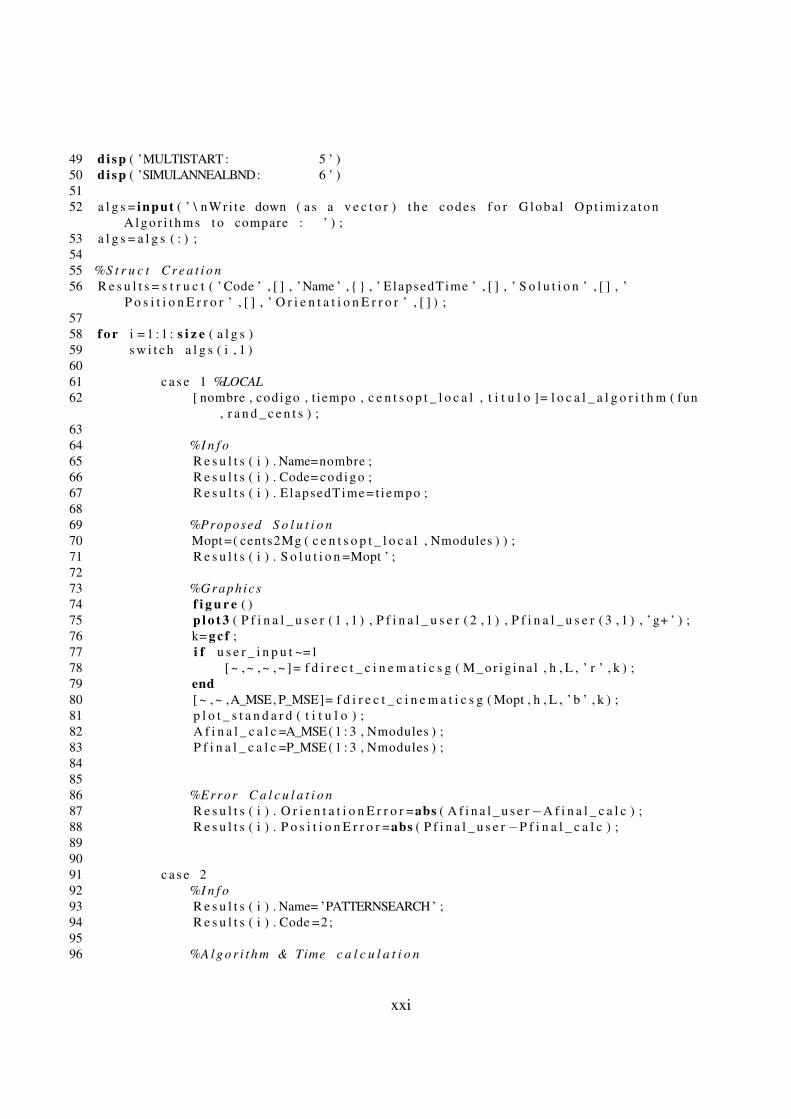
49 di sp ( ’MULTISTART : 5 ’ )50 di sp ( ’SIMULANNEALBND: 6 ’ )5152 a l g s = input ( ’ \ nWr i t e down ( as a v e c t o r ) t h e codes f o r G lo ba l O p t i m i z a t o n

A l g o r i t h m s t o compare : ’ ) ;53 a l g s = a l g s ( : ) ;5455 %S t r u c t C r e a t i o n56 R e s u l t s = s t r u c t ( ’ Code ’ , [ ] , ’Name ’ , { } , ’ ElapsedTime ’ , [ ] , ’ S o l u t i o n ’ , [ ] , ’

P o s i t i o n E r r o r ’ , [ ] , ’ O r i e n t a t i o n E r r o r ’ , [ ] ) ;5758 f o r i = 1 : 1 : s i z e ( a l g s )59 s w i t c h a l g s ( i , 1 )6061 c a s e 1 %LOCAL62 [ nombre , codigo , t iempo , c e n t s o p t _ l o c a l , t i t u l o ]= l o c a l _ a l g o r i t h m ( fun

, r a n d _ c e n t s ) ;6364 %I n f o65 R e s u l t s ( i ) . Name=nombre ;66 R e s u l t s ( i ) . Code= co d ig o ;67 R e s u l t s ( i ) . E lapsedTime = t iempo ;6869 %Proposed S o l u t i o n70 Mopt =( cents2Mg ( c e n t s o p t _ l o c a l , Nmodules ) ) ;71 R e s u l t s ( i ) . S o l u t i o n =Mopt ’ ;7273 %Graph ics74 f i g u r e ( )75 p l o t 3 ( P f i n a l _ u s e r ( 1 , 1 ) , P f i n a l _ u s e r ( 2 , 1 ) , P f i n a l _ u s e r ( 3 , 1 ) , ’ g+ ’ ) ;76 k= g c f ;77 i f u s e r _ i n p u t ~=178 [ ~ , ~ , ~ , ~ ] = f d i r e c t _ c i n e m a t i c s g ( M_or ig ina l , h , L , ’ r ’ , k ) ;79 end80 [ ~ , ~ ,A_MSE, P_MSE]= f d i r e c t _ c i n e m a t i c s g ( Mopt , h , L , ’ b ’ , k ) ;81 p l o t _ s t a n d a r d ( t i t u l o ) ;82 A f i n a l _ c a l c =A_MSE( 1 : 3 , Nmodules ) ;83 P f i n a l _ c a l c =P_MSE ( 1 : 3 , Nmodules ) ;848586 %Error C a l c u l a t i o n87 R e s u l t s ( i ) . O r i e n t a t i o n E r r o r =abs ( A f i n a l _ u s e r−A f i n a l _ c a l c ) ;88 R e s u l t s ( i ) . P o s i t i o n E r r o r =abs ( P f i n a l _ u s e r−P f i n a l _ c a l c ) ;899091 c a s e 292 %I n f o93 R e s u l t s ( i ) . Name= ’PATTERNSEARCH ’ ;94 R e s u l t s ( i ) . Code =2;9596 %A l g o r i t h m & Time c a l c u l a t i o n

xxi

97 tic_PATTERNSEARCH= t i c ;98 [ c e n t s o p t _ p a t t e r n s e a r c h , ~ , ~ , ~ ] = p a t t e r n s e a r c h ( fun , r a n d _ c e n t s

, [ ] , [ ] , [ ] , [ ] , z e r o s ( s e t s , 1 ) , ones ( s e t s , 1 ) ) ;99 R e s u l t s ( i ) . E lapsedTime = t o c ( tic_PATTERNSEARCH ) ;

100101 %Proposed S o l u t i o n102 Mopt =( cents2Mg ( c e n t s o p t _ p a t t e r n s e a r c h , Nmodules ) ) ;103 R e s u l t s ( i ) . S o l u t i o n =Mopt ’ ;104105 %Graph ics106 f i g u r e ( )107 p l o t 3 ( P f i n a l _ u s e r ( 1 , 1 ) , P f i n a l _ u s e r ( 2 , 1 ) , P f i n a l _ u s e r ( 3 , 1 ) , ’ g+ ’ ) ;108 k= g c f ;109 i f u s e r _ i n p u t ~=1110 [ ~ , ~ , ~ , ~ ] = f d i r e c t _ c i n e m a t i c s g ( M_or ig ina l , h , L , ’ r ’ , k ) ;111 end112 [ ~ , ~ ,A_MSE, P_MSE]= f d i r e c t _ c i n e m a t i c s g ( Mopt , h , L , ’ b ’ , k ) ;113 p l o t _ s t a n d a r d ( ’ S o l u t i o n wi th PATTERNSEARCH ’ ) ;114 A f i n a l _ c a l c =A_MSE( 1 : 3 , Nmodules ) ;115 P f i n a l _ c a l c =P_MSE ( 1 : 3 , Nmodules ) ;116117 %Error C a l c u l a t i o n118 R e s u l t s ( i ) . O r i e n t a t i o n E r r o r =abs ( A f i n a l _ u s e r−A f i n a l _ c a l c ) ;119 R e s u l t s ( i ) . P o s i t i o n E r r o r =abs ( P f i n a l _ u s e r−P f i n a l _ c a l c ) ;120121122 c a s e 3123 %I n f o124 R e s u l t s ( i ) . Name= ’GENETIC ALGORITHM’ ;125 R e s u l t s ( i ) . Code =3;126127 %Problem D e s c r i p t i o n128129 %A l g o r i t h m & Time c a l c u l a t i o n130 tic_GA= t i c ;131 [ c e n t s o p t _ g e n e t i c a l g o r i t h m , ~ ] = ga ( fun , s e t s , [ ] , [ ] , [ ] , [ ] , z e r o s ( s e t s

, 1 ) , ones ( s e t s , 1 ) ) ;132 R e s u l t s ( i ) . E lapsedTime = t o c ( t ic_GA ) ;133134 %Proposed S o l u t i o n135 Mopt =( cents2Mg ( c e n t s o p t _ g e n e t i c a l g o r i t h m , Nmodules ) ) ;136 R e s u l t s ( i ) . S o l u t i o n =Mopt ’ ;137138 %Graph ics139 f i g u r e ( )140 p l o t 3 ( P f i n a l _ u s e r ( 1 , 1 ) , P f i n a l _ u s e r ( 2 , 1 ) , P f i n a l _ u s e r ( 3 , 1 ) , ’ g+ ’ ) ;141 k= g c f ;142 i f u s e r _ i n p u t ~=1143 [ ~ , ~ , ~ , ~ ] = f d i r e c t _ c i n e m a t i c s g ( M_or ig ina l , h , L , ’ r ’ , k ) ;144 end145 [ ~ , ~ ,A_MSE, P_MSE]= f d i r e c t _ c i n e m a t i c s g ( Mopt , h , L , ’ b ’ , k ) ;

xxii

146 p l o t _ s t a n d a r d ( ’ S o l u t i o n wi th GENETIC ALGORITHM’ ) ;147 A f i n a l _ c a l c =A_MSE( 1 : 3 , Nmodules ) ;148 P f i n a l _ c a l c =P_MSE ( 1 : 3 , Nmodules ) ;149150 %Error C a l c u l a t i o n151 R e s u l t s ( i ) . O r i e n t a t i o n E r r o r =abs ( A f i n a l _ u s e r−A f i n a l _ c a l c ) ;152 R e s u l t s ( i ) . P o s i t i o n E r r o r =abs ( P f i n a l _ u s e r−P f i n a l _ c a l c ) ;153154155 c a s e 4156 %I n f o157 R e s u l t s ( i ) . Name= ’GLOBALSEARCH’ ;158 R e s u l t s ( i ) . Code =4;159160 %Problem D e s c r i p t i o n161 problem = c r e a t e O p t i m P r o b l e m ( ’ fmincon ’ , ’ o b j e c t i v e ’ , fun , ’ x0 ’ ,

r a n d _ c e n t s , ’ l b ’ , z e r o s ( s e t s , 1 ) , ’ ub ’ , ones ( s e t s , 1 ) ) ;162 gs= G l o b a l S e a r c h ;163164 %A l g o r i t h m & Time c a l c u l a t i o n165 tic_GLOBALSEARCH= t i c ;166 [ c e n t s o p t _ g l o b a l s e a r c h , ~ , ~ , ~ ] = run ( gs , problem ) ;167 R e s u l t s ( i ) . E lapsedTime = t o c ( tic_GLOBALSEARCH ) ;168169 %Proposed S o l u t i o n170 Mopt =( cents2Mg ( c e n t s o p t _ g l o b a l s e a r c h , Nmodules ) ) ;171 R e s u l t s ( i ) . S o l u t i o n =Mopt ’ ;172173 %Graph ics174 f i g u r e ( )175 p l o t 3 ( P f i n a l _ u s e r ( 1 , 1 ) , P f i n a l _ u s e r ( 2 , 1 ) , P f i n a l _ u s e r ( 3 , 1 ) , ’ g+ ’ ) ;176 k= g c f ;177 i f u s e r _ i n p u t ~=1178 [ ~ , ~ , ~ , ~ ] = f d i r e c t _ c i n e m a t i c s g ( M_or ig ina l , h , L , ’ r ’ , k ) ;179 end180 [ ~ , ~ ,A_MSE, P_MSE]= f d i r e c t _ c i n e m a t i c s g ( Mopt , h , L , ’ b ’ , k ) ;181 p l o t _ s t a n d a r d ( ’ S o l u t i o n wi th GLOBALSEARCH’ ) ;182 A f i n a l _ c a l c =A_MSE( 1 : 3 , Nmodules ) ;183 P f i n a l _ c a l c =P_MSE ( 1 : 3 , Nmodules ) ;184185 %Error C a l c u l a t i o n186 R e s u l t s ( i ) . O r i e n t a t i o n E r r o r =abs ( A f i n a l _ u s e r−A f i n a l _ c a l c ) ;187 R e s u l t s ( i ) . P o s i t i o n E r r o r =abs ( P f i n a l _ u s e r−P f i n a l _ c a l c ) ;188189190 c a s e 5191 %Problem D e s c r i p t i o n192 di sp ( ’ ’ )193 di sp ( ’ ’ )194 di sp ( ’ Code : ’ )195 di sp ( ’ ’ )

xxiii

196 di sp ( ’FMINUNC: 1 ’ )197 di sp ( ’LSQNONLIN : 2 ’ )198 g l o b a l _ t y p e = input ( ’ \ n \ nWr i t e down t h e code f o r MULTISTART

Algor i t hm t o compare : ’ ) ;199200 s w i t c h g l o b a l _ t y p e201 c a s e 1202 problem = c r e a t e O p t i m P r o b l e m ( ’ fminunc ’ , ’ o b j e c t i v e ’ , fun , ’ x0

’ , r a n d _ c e n t s ) ;203 R e s u l t s ( i ) . Name= ’MULTISTART : fminunc ’ ;204 R e s u l t s ( i ) . Code = 5 . 1 ;205 t i t u l o = ’ S o l u t i o n wi th MULTISTAR : fminunc ’ ;206 c a s e 2207 problem = c r e a t e O p t i m P r o b l e m ( ’ l s q n o n l i n ’ , ’ o b j e c t i v e ’ , fun , ’

x0 ’ , r a n d _ c e n t s ) ;208 R e s u l t s ( i ) . Name= ’MULTISTART : l s q n o n l i n ’ ;209 R e s u l t s ( i ) . Code = 5 . 2 ;210 t i t u l o = ’ S o l u t i o n wi th MULTISTAR : l s q n o n l i n ’ ;211 o t h e r w i s e212 di sp ( ’ E r r o r : No MULTISTART Algor i t hm S e l e c t e d ’ ) ;213 end214215 ms= M u l t i S t a r t ;216217 %A l g o r i t h m & Time c a l c u l a t i o n218 tic_MULTISTART= t i c ;219 [ c e n t s o p t _ m u l t i s t a r t , ~ , ~ , ~ , ~ ] = run ( ms , problem , 5 0 ) ;220 R e s u l t s ( i ) . E lapsedTime = t o c ( tic_MULTISTART ) ;221222 %Proposed S o l u t i o n223 Mopt =( cents2Mg ( c e n t s o p t _ m u l t i s t a r t , Nmodules ) ) ;224 R e s u l t s ( i ) . S o l u t i o n =Mopt ’ ;225226 %Graph ics227 f i g u r e ( )228 p l o t 3 ( P f i n a l _ u s e r ( 1 , 1 ) , P f i n a l _ u s e r ( 2 , 1 ) , P f i n a l _ u s e r ( 3 , 1 ) , ’ g+ ’ ) ;229 k= g c f ;230 i f u s e r _ i n p u t ~=1231 [ ~ , ~ , ~ , ~ ] = f d i r e c t _ c i n e m a t i c s g ( M_or ig ina l , h , L , ’ r ’ , k ) ;232 end233 [ ~ , ~ ,A_MSE, P_MSE]= f d i r e c t _ c i n e m a t i c s g ( Mopt , h , L , ’ b ’ , k ) ;234 p l o t _ s t a n d a r d ( t i t u l o ) ;235 A f i n a l _ c a l c =A_MSE( 1 : 3 , Nmodules ) ;236 P f i n a l _ c a l c =P_MSE ( 1 : 3 , Nmodules ) ;237238 %Error C a l c u l a t i o n239 R e s u l t s ( i ) . O r i e n t a t i o n E r r o r =abs ( A f i n a l _ u s e r−A f i n a l _ c a l c ) ;240 R e s u l t s ( i ) . P o s i t i o n E r r o r =abs ( P f i n a l _ u s e r−P f i n a l _ c a l c ) ;241242243 c a s e 6

xxiv

244 %I n f o245 R e s u l t s ( i ) . Name= ’SIMULANNEALBND’ ;246 R e s u l t s ( i ) . Code =6;247248 %A l g o r i t h m & Time c a l c u l a t i o n249 tic_SIMULANNEALBND= t i c ;250 [ c e n t s o p t _ s i m u l a n n e a l b n d , ~ ] = s i m u l a n n e a l b n d ( fun , r a n d _ c e n t s , z e r o s (

s e t s , 1 ) , ones ( s e t s , 1 ) ) ;251 R e s u l t s ( i ) . E lapsedTime = t o c ( tic_SIMULANNEALBND ) ;252253 %Proposed S o l u t i o n254 Mopt =( cents2Mg ( c e n t s o p t _ s i m u l a n n e a l b n d , Nmodules ) ) ;255 R e s u l t s ( i ) . S o l u t i o n =Mopt ’ ;256257 %Graph ics258 f i g u r e ( )259 p l o t 3 ( P f i n a l _ u s e r ( 1 , 1 ) , P f i n a l _ u s e r ( 2 , 1 ) , P f i n a l _ u s e r ( 3 , 1 ) , ’ g+ ’ ) ;260 k= g c f ;261 i f u s e r _ i n p u t ~=1262 [ ~ , ~ , ~ , ~ ] = f d i r e c t _ c i n e m a t i c s g ( M_or ig ina l , h , L , ’ r ’ , k ) ;263 end264 [ ~ , ~ ,A_MSE, P_MSE]= f d i r e c t _ c i n e m a t i c s g ( Mopt , h , L , ’ b ’ , k ) ;265 p l o t _ s t a n d a r d ( ’ S o l u t i o n wi th SIMULANNEALBND’ ) ;266 A f i n a l _ c a l c =A_MSE( 1 : 3 , Nmodules ) ;267 P f i n a l _ c a l c =P_MSE ( 1 : 3 , Nmodules ) ;268269 %Error C a l c u l a t i o n270 R e s u l t s ( i ) . O r i e n t a t i o n E r r o r =abs ( A f i n a l _ u s e r−A f i n a l _ c a l c ) ;271 R e s u l t s ( i ) . P o s i t i o n E r r o r =abs ( P f i n a l _ u s e r−P f i n a l _ c a l c ) ;272273274 o t h e r w i s e275 di sp ( ’ E r r o r : No G lob a l O p t i m i z a t i o n Logar i thm S e l e c t e d ’ ) ;276 di sp ( ’ There i s an e r r o r on t h e Algo r i t hm S e l e c t i o n Code on i t em

# : ’ )277 di sp ( i )278 di sp ( ’ The i n v a l i d v a l u e you e n t e r e d was : ’ )279 di sp ( a l g s ( i , 1 ) )280281 end282283 end284285 Codes =[ R e s u l t s . Code ] ’ ;286 Names={ R e s u l t s . Name } ’ ;287 ElapsedTimes =[ R e s u l t s . E lapsedTime ] ’ ;288 S o l u t i o n s =[ R e s u l t s . S o l u t i o n ] ;289 P o s i t i o n E r r o r s =[ R e s u l t s . P o s i t i o n E r r o r ] ;290 O r i e n t a t i o n E r r o r s =[ R e s u l t s . O r i e n t a t i o n E r r o r ] ;291 PPTimes =[ Codes ElapsedTimes ] ;

xxv

Forward Kinematics

1 %%S c r i p t t o c a l c u l a t e t h e Forward K i n e m a t i c s o f t h e HRRS23 c l e a r a l l ; %c l e a r o f v a r i a b l e s4 c l o s e a l l ; %c l o s e a l l windows5 c l c ; %Workspace c l e a r67 %{8 %FOR FORWARD CINEMATICS9

10 %2−−−−3−−−−111 %| | |12 %6−−−0/15−−913 %| | |14 %4−−−−12−−−815161718 [0 0 1 0]−−−−−[0 0 1 1]−−−−−[0 0 0 1]19 | |20 | |21 | |22 | [0 0 0 0] |23 [0 1 1 0]−−−−−+++++++++−−−−−[1 0 0 1]24 | [1 1 1 1] |25 | |26 | |27 | |28 [0 1 0 0]−−−−−[1 1 0 0]−−−−−[1 0 0 0]2930 %}3132 %%S c r i p t f o r D i r e c t C i n e m a t i c s3334 di sp ( ’ S c r i p t f o r Forward K i n e m a t i c s ’ )35 di sp ( ’ ’ )3637 %PHYSICAL PARAMETERS38 h= input ( ’ \ nMinimum s p a c e between modules (m) ? : ’ ) ;39 L= input ( ’ \ nLength o f each module (m) ? : ’ ) ;404142 u s e r _ r o b o t = input ( ’ \ n P r e s s ’ ’ 0 ’ ’ f o r Random Robot , ’ ’ 1 ’ ’ f o r use r−i n p u t r o b o t

: ’ ) ;4344 i f u s e r _ r o b o t ==045 Nmodules= input ( ’ \ nNumber o f Modules ? : ’ ) ;46 M p l a t e s d e c = c r e a t e _ m o d _ r o b o t 2 ( Nmodules ) ;47 Mpla t e s = d e c b i n ( M p l a t e s d e c ) ;48 g o _ f l a g =1;

xxvi

49 e l s e50 M= input ( ’ \ nWr i t e down each one of t h e modules c o n f i g u r a t i o n as a d e c i m a l

number i n a column or row v e c t o r o r a s a b i n a r y m a t r i x were each rowr e p r e s e n t s a module : ’ ) ;

51 Mpla t e s = d e c b i n (M) ;%T r a n s l a t i n g t h e i n p u t m a t r i x t o b i n a r y code52 M p l a t e s d e c = b i 2 d e ( Mpla tes , ’ l e f t −msb ’ ) ; %For c h e c k i n g t h e d e c i m a l MC53 g o _ f l a g = e r r o r c h e c k ( Mpla t e s ) ;%Check ing f o r e r r o r s54 end555657 i f g o _ f l a g ==1%T h i s means t h e r e weren ’ t any non a c c e p t e d module

c o n f i g u r a t i o n s5859 %M a t h e m a t i c a l c o n v e r s i o n60 Mangles= c o n v e r s o r ( Mpla tes , h , L ) ;%C o n v e r t i n g t h e b i n a r y row v e c t o r code t o

a lpha and t h e t a a n g l e s6162 %NOAP C a l c u l a t i o n63 Final_MSE=calculate_NOAP_MSE ( Mangles ) ;%C a l c u l a t i n g t h e NOAP f o r each

module64 [N_MSE, O_MSE, A_MSE, P_MSE]= NOAP_vects ( Final_MSE ) ;%P r e t t y P r i n t o u t p u t /

Comparison6566 e l s e67 di sp ( ’ There i s an e r r o r . Go t o ∗ e r r o r c h e c k ∗ f o r non−a c c e p t e d

c o m b i n a t i o n s ’ ) ;68 end

xxvii

Homo Rot Mat Any

1 f u n c t i o n T _ r o t =homo_rot_mat_any ( r o t _ a n g l e , r o t _ a x i s _ v e c t )2 %%F u n c t i o n t o c a l c u l a t e t h e homogeneous r o t a t i o n m a t r i x w i t h r o t a t i o n a x i s

d e s c r i b e d by ’ r o t _ a x i s _ v e c t ’ over a c e r t a i n r o t a t i o n a n g l e ’ r o t _ a n g l e ’ .34 %P r e a l l o c a t i o n5 T_ro t_1 = z e r o s ( 3 ) ;6 T _ r o t = z e r o s ( 4 ) ;78 u n i t _ r o t _ a x i s _ v e c t = r o t _ a x i s _ v e c t / ( norm ( r o t _ a x i s _ v e c t ) ) ;%N o r m a l i z i n g

v e c t o r9

10 u= u n i t _ r o t _ a x i s _ v e c t ( 1 , 1 ) ;11 v= u n i t _ r o t _ a x i s _ v e c t ( 1 , 2 ) ;12 w= u n i t _ r o t _ a x i s _ v e c t ( 1 , 3 ) ;1314 %Va lu es15 u2=u ^ 2 ;16 v2=v ^ 2 ;17 w2=w^ 2 ;18 c= cos ( r o t _ a n g l e ) ;19 s= s i n ( r o t _ a n g l e ) ;2021 %F i l l i n g t h e m a t r i x22 T_ro t_1 ( 1 , 1 ) =u2 + ( v2 + w2 ) ∗c ;23 T_ro t_1 ( 1 , 2 ) =u∗v∗(1−c ) − w∗ s ;24 T_ro t_1 ( 1 , 3 ) =u∗w∗(1−c ) + v∗ s ;25 T_ro t_1 ( 2 , 1 ) =u∗v∗(1−c ) + w∗ s ;26 T_ro t_1 ( 2 , 2 ) =v2 + ( u2+w2 ) ∗c ;27 T_ro t_1 ( 2 , 3 ) =v∗w∗(1−c ) − u∗ s ;28 T_ro t_1 ( 3 , 1 ) =u∗w∗(1−c ) − v∗ s ;29 T_ro t_1 ( 3 , 2 ) =v∗w∗(1−c ) +u∗ s ;30 T_ro t_1 ( 3 , 3 ) =w2 + ( u2+v2 ) ∗c ;3132 T _ r o t ( 4 , 4 ) =1 ;33 T _ r o t ( 1 : 3 , 1 : 3 ) = T_ro t_1 ;343536 end

xxviii

Homo Trans Mat

1 f u n c t i o n [ T _ t r a n s ]= homo_t rans_mat ( v e c t )2 %%F u n c t i o n t o c a l c u l a t e t h e t r a n s l a t i o n m a t r i x f o r any 3D v e c t o r34 %{5 [ 1 0 0 v e c t x6 0 1 0 v e c t y7 0 0 1 v e c t z8 0 0 0 1 ]9 %}

1011 i f s i z e ( vec t , 1 ) <112 di sp ( ’ Must be a 3D v e c t o r ’ )13 e l s e14 T _ t r a n s =eye ( 4 ) ;15 T _ t r a n s ( 1 : 3 , 4 ) = vec t ’ ;16 end1718 end

xxix

Inverse Kinematics

1 %%S c r i p t t o c a l c u l a t e t h e i n v e r s e k i n e m a t i c s o f t h e HRRS based on e x h a u s t i v e( f o r l e s s or e q u a l t o 3 modules ) or e r r o r−o p t i m i z a t i o n methods

23 c l c ;4 c l o s e a l l ;5 c l e a r a l l ;67 %PHYSICAL PARAMETERS8 h= input ( ’ \ nMinimum s p a c e between modules (m) ? : ’ ) ;9 L= input ( ’ \ nLength o f each module (m) ? : ’ ) ;

10 Nmodules= input ( ’ \ nNumber o f Modules ? : ’ ) ;1112 i f Nmodules >=413 modo =2;14 e l s e15 modo =1;16 end1718 s w i t c h modo19 c a s e 120 Mopt= f e x h a u s t i v e ( h , L , Nmodules ) ;2122 c a s e 223 Mopt= f o p t i m i z a t i o n ( h , L , Nmodules ) ;2425 o t h e r w i s e26 di sp ( ’You d i d n o t s e l e c t a v a l i d Method ’ ) ;27 end

xxx

Local Algorithm

1 f u n c t i o n [ nombre , codigo , t iempo , c e n t s o p t _ l o c a l , t i t u l o ]= l o c a l _ a l g o r i t h m ( fun ,r a n d _ c e n t s )

2 %%F u n c t i o n t o s e l e c t and c a l c u l a t e t h e i n v e r s e k i n e m a t i c s based on a l o c a le r r o r−o p t i m i z a t i o n a l g o r i t h m

34 %A l g o r i t h m S e l e c t i o n & Time c a l c u l a t i o n5 di sp ( ’ ’ )6 di sp ( ’ ’ )7 di sp ( ’ Code : ’ )8 di sp ( ’ ’ )9 di sp ( ’FMINUNC: 1 ’ )

10 di sp ( ’LSQNONLIN : 2 ’ )11 di sp ( ’FMINSEARCH: 3 ’ )121314 l o c a l _ t y p e = input ( ’ \ n \ nWr i t e down t h e code f o r Loca l O p t i m i z a t o n

Algo r i t hm t o compare : ’ ) ;15 s w i t c h l o c a l _ t y p e16 c a s e 1 %’ fminunc ’17 %I n f o18 nombre= ’LOCAL: fminunc ’ ;19 c od ig o = 1 . 1 ;20 t i t u l o = ’ S o l u t i o n wi th LOCAL: fminunc ’ ;2122 %Time c a l c u l a t i o n23 tic_LOCAL= t i c ;24 [ c e n t s o p t _ l o c a l , ~ , ~ , ~ ] = fminunc ( fun , r a n d _ c e n t s ) ;25 t i empo = t o c ( tic_LOCAL ) ;262728 c a s e 2 %’ l s q n o n l i n ’29 %I n f o30 nombre= ’LOCAL: l s q n o n l i n ’ ;31 c od ig o = 1 . 2 ;32 t i t u l o = ’ S o l u t i o n wi th LOCAL: l s q n o n l i n ’ ;3334 %Time c a l c u l a t i o n35 tic_LOCAL= t i c ;36 [ c e n t s o p t _ l o c a l , ~ , ~ , ~ ] = l s q n o n l i n ( fun , r a n d _ c e n t s ) ;37 t i empo = t o c ( tic_LOCAL ) ;383940 c a s e 3 %’ f m i n s e a r c h ’41 %I n f o42 nombre= ’LOCAL: f m i n s e a r c h ’ ;43 c od ig o = 1 . 3 ;44 t i t u l o = ’ S o l u t i o n wi th LOCAL: f m i n s e a r c h ’ ;4546 %Time c a l c u l a t i o n

xxxi

47 tic_LOCAL= t i c ;48 [ c e n t s o p t _ l o c a l , ~ , ~ , ~ ] = f m i n s e a r c h ( fun , r a n d _ c e n t s ) ;49 t i empo = t o c ( tic_LOCAL ) ;50515253 c a s e 4 %’ l s q c u r v e f i t ’54 nombre= ’LSQCURVEFIT ’ ;55 c od ig o = 1 . 4 ;56 tic_LOCAL= t i c ;57 [ c e n t s o p t _ l o c a l , ~ , ~ , ~ ] = l s q c u r v e f i t ( fun , r a n d _ c e n t s , [ ] , [ ] ) ;58 t i empo = t o c ( tic_LOCAL ) ;5960 %{61 c a s e 5 %’ fmincon ’62 nombre= ’FMINCON ’ ;63 c od ig o = 1 . 5 ;64 tic_LOCAL= t i c ;65 [ c e n t s o p t _ l o c a l , ~ , ~ , ~ ] = fmincon ( fun , r a n d _ c e n t s , [ ] , [ ] ) ;66 t i empo = t o c ( tic_LOCAL ) ;67 %}6869 %{70 c a s e 6 %’ f s e m i n f ’71 nombre= ’FSEMINF ’ ;72 c od ig o = 1 . 6 ;73 tic_LOCAL= t i c ;74 [ c e n t s o p t _ l o c a l , ~ , ~ , ~ ] = f s e m i n f ( fun , r a n d _ c e n t s ) ;75 t i empo = t o c ( tic_LOCAL ) ;76 %}7778 c a s e 7 %’ fminbnd ’ %S i n g l e−v a r i a b l e bounded n o n l i n e a r f u n c t i o n

m i n i m i z a t i o n .79 nombre= ’FMINBND ’ ;80 c od ig o = 1 . 7 ;81 tic_LOCAL= t i c ;82 [ c e n t s o p t _ l o c a l , ~ , ~ , ~ ] = fminbnd ( fun , [ 0 0 ] , [ 1 1 ] ) ;83 t i empo = t o c ( tic_LOCAL ) ;848586 o t h e r w i s e87 di sp ( ’ E r r o r : No Loca l O p t i m i z a t i o n Algo r i t hm S e l e c t e d ’ ) ;8889 end90 end

xxxii

M2Cents

1 f u n c t i o n c e n t =M2cents (M)2 %%F u n c t i o n t o c o n v e r t MC d e c i m a l code t o c e n t s (4 MCs a t a t i m e )34 c e n t =0 ;5 Nmodules= s i z e (M, 2 ) ;67 f o r i = 1 : 1 : Nmodules8 aux3=M( 1 , i ) ;9 s w i t c h aux3

10 c a s e 011 c e n t = c e n t + 0∗ ( 0 . 1 ^ i ) ;12 c a s e 113 c e n t = c e n t + 4∗ ( 0 . 1 ^ i ) ;14 c a s e 215 c e n t = c e n t + 6∗ ( 0 . 1 ^ i ) ;16 c a s e 317 c e n t = c e n t + 5∗ ( 0 . 1 ^ i ) ;18 c a s e 419 c e n t = c e n t + 8∗ ( 0 . 1 ^ i ) ;20 c a s e 621 c e n t = c e n t + 7∗ ( 0 . 1 ^ i ) ;22 c a s e 823 c e n t = c e n t + 2∗ ( 0 . 1 ^ i ) ;24 c a s e 925 c e n t = c e n t + 3∗ ( 0 . 1 ^ i ) ;26 c a s e 1227 c e n t = c e n t + 1∗ ( 0 . 1 ^ i ) ;28 c a s e 1529 c e n t = c e n t + 9∗ ( 0 . 1 ^ i ) ;30 end31 end3233 end

xxxiii

M2Cents G

1 f u n c t i o n c e n t s =M2centsg (M)2 %%F u n c t i o n as t h e g e n e r a l v e r s i o n o f M2cents34 M=M( : ) ’ ;%V e c t o r t r a n s f o r m i n t o column5 Nmodules= s i z e (M, 2 ) ;67 s e t s = c e i l ( Nmodules / 4 ) ;89 M p a r c i a l = z e r o s ( 1 , s e t s ∗4) ;

10 c e n t s = z e r o s ( s e t s , 1 ) ;1112 M p a r c i a l ( 1 , 1 : Nmodules ) =M;13 M p a r c i a l = reshape ( Mparc ia l , 4 , [ ] ) ’ ;141516 f o r i = 1 : 1 : s e t s17 c e n t s ( i , 1 ) =M2cents ( M p a r c i a l ( i , 1 : 4 ) ) ;18 end1920 end

xxxiv

NOAP Calc

1 f u n c t i o n Final_MSE=NOAP_calc (M, h , L )2 %%T h i s f u n c t i o n c a l c u l a t e s NOAP v e c t o r s w i t h o u t any p l o t t i n g i n v o l v e d3 %Mangles ( : , 1 ) =Alpha4 %Mangles ( : , 2 ) =The ta5 %Mangles ( : , 3 ) =h6 %Mangles ( : , 4 ) =L78 Mpla t e s = d e c b i n (M) ; %T r a n s l a t i n g t h e i n p u t m a t r i x t o b i n a r y code9 Mangles= c o n v e r s o r ( Mpla tes , h , L ) ; %C o n v e r t i n g t h e b i n a r y row v e c t o r code

t o a lpha and t h e t a a n g l e s1011 Nmodules= s i z e ( Mangles , 1 ) ; %Number o f Modules1213 P0=eye ( 4 ) ; %I n i t i a l i z a t i o n f o r NOAP c a l c u l a t i o n1415 f o r i = 1 : 1 : Nmodules %NOAP c a l c u l a t i o n f o r each one o f t h e modules1617 %NOAP C a l c u l a t i o n18 P1=P0∗ homo_rot_mat_any ( Mangles ( i , 2 ) , [ 0 0 1 ] ) ;19 P2=P1∗ homo_t rans_mat ( [ 0 0 Mangles ( i , 3 ) ] ) ;20 P3=P2∗ homo_rot_mat_any ( ( Mangles ( i , 1 ) / 2 ) , [ 1 0 0 ] ) ;21 P4=P3∗ homo_t rans_mat ( [ 0 0 Mangles ( i , 4 ) ∗ s i n ( Mangles ( i , 1 ) / 2 ) ] ) ;22 P5=P4∗ homo_rot_mat_any ( ( Mangles ( i , 1 ) / 2 ) , [ 1 0 0 ] ) ;23 P6=P5∗ homo_rot_mat_any (−( Mangles ( i , 2 ) ) , [ 0 0 1 ] ) ;24 P u n i t = u n i t _ v e c t o r _ m a t ( P6 ) ;25 Final_MSE ( i ∗4−3: i ∗4 , i ∗4−3: i ∗4) = P u n i t ;26 P0= P u n i t ;2728 end2930 end

xxxv

NOAP Vects

1 f u n c t i o n [ N_vect , O_vect , A_vect , P _ve c t ]= NOAP_vects ( F i n a l )2 %%T h i s f u n c t i o n c a l c u l a t e s NOAP v e c t o r s f o r any ’ F ina l ’ m a t r i x34 F i n a l _ s i z e = s i z e ( F i n a l , 1 ) ;56 N_vect ( 1 : 3 , 1 ) = F i n a l ( 1 : 3 , 1 ) ;7 O_vect ( 1 : 3 , 1 ) = F i n a l ( 1 : 3 , 2 ) ;8 A_vect ( 1 : 3 , 1 ) = F i n a l ( 1 : 3 , 3 ) ;9 P _v ec t ( 1 : 3 , 1 ) = F i n a l ( 1 : 3 , 4 ) ;

101112 f o r j = 1 : 1 : F i n a l _ s i z e /4−11314 N_vect ( 1 : 3 , j +1)= F i n a l ( j ∗4+1: j ∗4+1+2 , j ∗4+1) ;15 O_vect ( 1 : 3 , j +1)= F i n a l ( j ∗4+1: j ∗4+1+2 , j ∗4+2) ;16 A_vect ( 1 : 3 , j +1)= F i n a l ( j ∗4+1: j ∗4+1+2 , j ∗4+3) ;17 P _v ec t ( 1 : 3 , j +1)= F i n a l ( j ∗4+1: j ∗4+1+2 , j ∗4+4) ;1819 end2021 end

xxxvi

Optimization

1 %%S c r i p t t o c a l c u l a t e t h e i n v e r s e k i n e m a t i c s t h r o u g h e r r o r−o p t i m i z a t i o nmethod

23 c l c ;4 c l o s e a l l ;5 c l e a r a l l ;67 %PHYSICAL PARAMETERS8 h= input ( ’ \ nMinimum s p a c e between modules (m) ? : ’ ) ;9 L= input ( ’ \ nLength o f each module (m) ? : ’ ) ;

10 Nmodules= input ( ’ \ nNumber o f Modules ? : ’ ) ;11 s e t s = c e i l ( Nmodules / 4 ) ;1213 u s e r _ i n p u t = input ( ’Do you want a random c a s e ( 0 ) o r use r−i n p u t ( 1 ) ? : ’ ) ;141516 %FINAL PARAMETERS17 i f u s e r _ i n p u t ==1%For s p e c i f i c case18 P f i n a l _ u s e r = input ( ’ \ n F i n a l D e s t i n a t i o n P o i n t : ’ ) ;19 P f i n a l _ u s e r = P f i n a l _ u s e r ( : ) ;20 A f i n a l _ u s e r = input ( ’ \ n F i n a l O r i e n t a t i o n : ’ ) ;21 A f i n a l _ u s e r = A f i n a l _ u s e r ( : ) ;22 A f i n a l _ u s e r = A f i n a l _ u s e r / norm ( A f i n a l _ u s e r ) ;2324 e l s e%For Random case25 M _ o r i g i n a l = c r e a t e _ m o d _ r o b o t 2 ( Nmodules ) ;26 F i n a l _ i n t =NOAP_calc ( M_or ig ina l , h , L ) ;27 [ ~ , ~ , A_vect , P_v ec t ]= NOAP_vects ( F i n a l _ i n t ) ;28 A f i n a l _ u s e r =A_vect ( 1 : 3 , Nmodules ) ;29 P f i n a l _ u s e r = P_v ec t ( 1 : 3 , Nmodules ) ;30 c e n t s _ o r i g i n a l =M2centsg ( M _ o r i g i n a l ) ;3132 end333435 %INITIAL POINT CALCULATION36 r a n d _ r o b o t = c r e a t e _ m o d _ r o b o t 2 ( Nmodules ) ;37 primmodM= d i r _ c a l c 2 ( P f i n a l _ u s e r , 0 . 0 0 0 0 1 ) ;38 primmodC=M2cents ( primmodM ) ;39 r a n d _ r o b o t ( 1 ) =primmodM ; %Ayuda d e l pr imero modulo c a l c u l a d o40 r a n d _ c e n t s =M2centsg ( r a n d _ r o b o t ) ;414243 %TARGET FUNCTION (FOR OPTIMIZATION )44 fun =@( c e n t s ) c a l c _ e r r o r ( c e n t s , P f i n a l _ u s e r , A f i n a l _ u s e r , Nmodules , h , L ) ;454647 %OPTIMIZATION PROCEDURE48 di sp ( ’ ’ )

xxxvii

49 di sp ( ’ ’ )50 di sp ( ’ Code : ’ )51 di sp ( ’ ’ )52 di sp ( ’LOCAL: 1 ’ )53 di sp ( ’PATTERNSEARCH: 2 ’ )54 di sp ( ’GENETIC ALGORITHM: 3 ’ )55 di sp ( ’GLOBALSEARCH: 4 ’ )56 di sp ( ’MULTISTART : 5 ’ )57 di sp ( ’SIMULANNEALBND: 6 ’ )5859 a l g s = input ( ’ \ nWr i t e down ( as a v e c t o r ) t h e codes f o r G lo ba l O p t i m i z a t o n

A l g o r i t h m s t o compare : ’ ) ;60 a l g s = a l g s ( : ) ;6162 %S t r u c t C r e a t i o n63 R e s u l t s = s t r u c t ( ’ Code ’ , [ ] , ’Name ’ , { } , ’ ElapsedTime ’ , [ ] , ’ S o l u t i o n ’ , [ ] , ’

P o s i t i o n E r r o r ’ , [ ] , ’ O r i e n t a t i o n E r r o r ’ , [ ] ) ;6465 f o r i = 1 : 1 : s i z e ( a l g s )66 s w i t c h a l g s ( i , 1 )6768 c a s e 1 %LOCAL69 [ nombre , codigo , t iempo , c e n t s o p t _ l o c a l , t i t u l o ]= l o c a l _ a l g o r i t h m ( fun

, r a n d _ c e n t s ) ;7071 %I n f o72 R e s u l t s ( i ) . Name=nombre ;73 R e s u l t s ( i ) . Code= co d ig o ;74 R e s u l t s ( i ) . E lapsedTime = t iempo ;7576 %Proposed S o l u t i o n77 Mopt =( cents2Mg ( c e n t s o p t _ l o c a l , Nmodules ) ) ;78 R e s u l t s ( i ) . S o l u t i o n =Mopt ’ ;7980 %Graph ics81 f i g u r e ( )82 p l o t 3 ( P f i n a l _ u s e r ( 1 , 1 ) , P f i n a l _ u s e r ( 2 , 1 ) , P f i n a l _ u s e r ( 3 , 1 ) , ’ r + ’ ) ;83 k= g c f ;84 i f u s e r _ i n p u t ~=185 [ ~ , ~ , ~ , ~ ] = f d i r e c t _ c i n e m a t i c s g ( M_or ig ina l , h , L , ’ r ’ , k ) ;86 end87 [ ~ , ~ ,A_MSE, P_MSE]= f d i r e c t _ c i n e m a t i c s g ( Mopt , h , L , ’ b ’ , k ) ;88 p l o t _ s t a n d a r d ( t i t u l o ) ;89 A f i n a l _ c a l c =A_MSE( 1 : 3 , Nmodules ) ;90 P f i n a l _ c a l c =P_MSE ( 1 : 3 , Nmodules ) ;919293 %Error C a l c u l a t i o n94 R e s u l t s ( i ) . O r i e n t a t i o n E r r o r =abs ( A f i n a l _ u s e r−A f i n a l _ c a l c ) ;95 R e s u l t s ( i ) . P o s i t i o n E r r o r =abs ( P f i n a l _ u s e r−P f i n a l _ c a l c ) ;96

xxxviii

9798 c a s e 299 %I n f o

100 R e s u l t s ( i ) . Name= ’PATTERNSEARCH ’ ;101 R e s u l t s ( i ) . Code =2;102103 %A l g o r i t h m & Time c a l c u l a t i o n104 tic_PATTERNSEARCH= t i c ;105 [ c e n t s o p t _ p a t t e r n s e a r c h , ~ , ~ , ~ ] = p a t t e r n s e a r c h ( fun , r a n d _ c e n t s

, [ ] , [ ] , [ ] , [ ] , z e r o s ( s e t s , 1 ) , ones ( s e t s , 1 ) ) ;106 R e s u l t s ( i ) . E lapsedTime = t o c ( tic_PATTERNSEARCH ) ;107108 %Proposed S o l u t i o n109 Mopt =( cents2Mg ( c e n t s o p t _ p a t t e r n s e a r c h , Nmodules ) ) ;110 R e s u l t s ( i ) . S o l u t i o n =Mopt ’ ;111112 %Graph ics113 f i g u r e ( )114 p l o t 3 ( P f i n a l _ u s e r ( 1 , 1 ) , P f i n a l _ u s e r ( 2 , 1 ) , P f i n a l _ u s e r ( 3 , 1 ) , ’ r + ’ ) ;115 k= g c f ;116 i f u s e r _ i n p u t ~=1117 [ ~ , ~ , ~ , ~ ] = f d i r e c t _ c i n e m a t i c s g ( M_or ig ina l , h , L , ’ r ’ , k ) ;118 end119 [ ~ , ~ ,A_MSE, P_MSE]= f d i r e c t _ c i n e m a t i c s g ( Mopt , h , L , ’ b ’ , k ) ;120 p l o t _ s t a n d a r d ( ’ S o l u t i o n wi th PATTERNSEARCH ’ ) ;121 A f i n a l _ c a l c =A_MSE( 1 : 3 , Nmodules ) ;122 P f i n a l _ c a l c =P_MSE ( 1 : 3 , Nmodules ) ;123124 %Error C a l c u l a t i o n125 R e s u l t s ( i ) . O r i e n t a t i o n E r r o r =abs ( A f i n a l _ u s e r−A f i n a l _ c a l c ) ;126 R e s u l t s ( i ) . P o s i t i o n E r r o r =abs ( P f i n a l _ u s e r−P f i n a l _ c a l c ) ;127128129 c a s e 3130 %I n f o131 R e s u l t s ( i ) . Name= ’GENETIC ALGORITHM’ ;132 R e s u l t s ( i ) . Code =3;133134 %Problem D e s c r i p t i o n135136 %A l g o r i t h m & Time c a l c u l a t i o n137 tic_GA= t i c ;138 [ c e n t s o p t _ g e n e t i c a l g o r i t h m , ~ ] = ga ( fun , s e t s , [ ] , [ ] , [ ] , [ ] , z e r o s ( s e t s

, 1 ) , ones ( s e t s , 1 ) ) ;139 R e s u l t s ( i ) . E lapsedTime = t o c ( t ic_GA ) ;140141 %Proposed S o l u t i o n142 Mopt =( cents2Mg ( c e n t s o p t _ g e n e t i c a l g o r i t h m , Nmodules ) ) ;143 R e s u l t s ( i ) . S o l u t i o n =Mopt ’ ;144145 %Graph ics

xxxix

146 f i g u r e ( )147 p l o t 3 ( P f i n a l _ u s e r ( 1 , 1 ) , P f i n a l _ u s e r ( 2 , 1 ) , P f i n a l _ u s e r ( 3 , 1 ) , ’ r + ’ ) ;148 k= g c f ;149 i f u s e r _ i n p u t ~=1150 [ ~ , ~ , ~ , ~ ] = f d i r e c t _ c i n e m a t i c s g ( M_or ig ina l , h , L , ’ r ’ , k ) ;151 end152 [ ~ , ~ ,A_MSE, P_MSE]= f d i r e c t _ c i n e m a t i c s g ( Mopt , h , L , ’ b ’ , k ) ;153 p l o t _ s t a n d a r d ( ’ S o l u t i o n wi th GENETIC ALGORITHM’ ) ;154 A f i n a l _ c a l c =A_MSE( 1 : 3 , Nmodules ) ;155 P f i n a l _ c a l c =P_MSE ( 1 : 3 , Nmodules ) ;156157 %Error C a l c u l a t i o n158 R e s u l t s ( i ) . O r i e n t a t i o n E r r o r =abs ( A f i n a l _ u s e r−A f i n a l _ c a l c ) ;159 R e s u l t s ( i ) . P o s i t i o n E r r o r =abs ( P f i n a l _ u s e r−P f i n a l _ c a l c ) ;160161162 c a s e 4163 %I n f o164 R e s u l t s ( i ) . Name= ’GLOBALSEARCH’ ;165 R e s u l t s ( i ) . Code =4;166167 %Problem D e s c r i p t i o n168 problem = c r e a t e O p t i m P r o b l e m ( ’ fmincon ’ , ’ o b j e c t i v e ’ , fun , ’ x0 ’ ,

r a n d _ c e n t s , ’ l b ’ , z e r o s ( s e t s , 1 ) , ’ ub ’ , ones ( s e t s , 1 ) ) ;169 gs= G l o b a l S e a r c h ;170171 %A l g o r i t h m & Time c a l c u l a t i o n172 tic_GLOBALSEARCH= t i c ;173 [ c e n t s o p t _ g l o b a l s e a r c h , ~ , ~ , ~ ] = run ( gs , problem ) ;174 R e s u l t s ( i ) . E lapsedTime = t o c ( tic_GLOBALSEARCH ) ;175176 %Proposed S o l u t i o n177 Mopt =( cents2Mg ( c e n t s o p t _ g l o b a l s e a r c h , Nmodules ) ) ;178 R e s u l t s ( i ) . S o l u t i o n =Mopt ’ ;179180 %Graph ics181 f i g u r e ( )182 p l o t 3 ( P f i n a l _ u s e r ( 1 , 1 ) , P f i n a l _ u s e r ( 2 , 1 ) , P f i n a l _ u s e r ( 3 , 1 ) , ’ r + ’ ) ;183 k= g c f ;184 i f u s e r _ i n p u t ~=1185 [ ~ , ~ , ~ , ~ ] = f d i r e c t _ c i n e m a t i c s g ( M_or ig ina l , h , L , ’ r ’ , k ) ;186 end187 [ ~ , ~ ,A_MSE, P_MSE]= f d i r e c t _ c i n e m a t i c s g ( Mopt , h , L , ’ b ’ , k ) ;188 p l o t _ s t a n d a r d ( ’ S o l u t i o n wi th GLOBALSEARCH’ ) ;189 A f i n a l _ c a l c =A_MSE( 1 : 3 , Nmodules ) ;190 P f i n a l _ c a l c =P_MSE ( 1 : 3 , Nmodules ) ;191192 %Error C a l c u l a t i o n193 R e s u l t s ( i ) . O r i e n t a t i o n E r r o r =abs ( A f i n a l _ u s e r−A f i n a l _ c a l c ) ;194 R e s u l t s ( i ) . P o s i t i o n E r r o r =abs ( P f i n a l _ u s e r−P f i n a l _ c a l c ) ;195

xl

196197 c a s e 5198 %Problem D e s c r i p t i o n199 di sp ( ’ ’ )200 di sp ( ’ ’ )201 di sp ( ’ Code : ’ )202 di sp ( ’ ’ )203 di sp ( ’FMINUNC: 1 ’ )204 di sp ( ’LSQNONLIN : 2 ’ )205 g l o b a l _ t y p e = input ( ’ \ n \ nWr i t e down t h e code f o r MULTISTART

Algor i t hm t o compare : ’ ) ;206207 s w i t c h g l o b a l _ t y p e208 c a s e 1209 problem = c r e a t e O p t i m P r o b l e m ( ’ fminunc ’ , ’ o b j e c t i v e ’ , fun , ’ x0

’ , r a n d _ c e n t s ) ;210 R e s u l t s ( i ) . Name= ’MULTISTART : fminunc ’ ;211 R e s u l t s ( i ) . Code = 5 . 1 ;212 t i t u l o = ’ S o l u t i o n wi th MULTISTAR : fminunc ’ ;213 c a s e 2214 problem = c r e a t e O p t i m P r o b l e m ( ’ l s q n o n l i n ’ , ’ o b j e c t i v e ’ , fun , ’

x0 ’ , r a n d _ c e n t s ) ;215 R e s u l t s ( i ) . Name= ’MULTISTART : l s q n o n l i n ’ ;216 R e s u l t s ( i ) . Code = 5 . 2 ;217 t i t u l o = ’ S o l u t i o n wi th MULTISTAR : l s q n o n l i n ’ ;218 o t h e r w i s e219 di sp ( ’ E r r o r : No MULTISTART Algor i t hm S e l e c t e d ’ ) ;220 end221222 ms= M u l t i S t a r t ;223224 %A l g o r i t h m & Time c a l c u l a t i o n225 tic_MULTISTART= t i c ;226 [ c e n t s o p t _ m u l t i s t a r t , ~ , ~ , ~ , ~ ] = run ( ms , problem , 5 0 ) ;227 R e s u l t s ( i ) . E lapsedTime = t o c ( tic_MULTISTART ) ;228229 %Proposed S o l u t i o n230 Mopt =( cents2Mg ( c e n t s o p t _ m u l t i s t a r t , Nmodules ) ) ;231 R e s u l t s ( i ) . S o l u t i o n =Mopt ’ ;232233 %Graph ics234 f i g u r e ( )235 p l o t 3 ( P f i n a l _ u s e r ( 1 , 1 ) , P f i n a l _ u s e r ( 2 , 1 ) , P f i n a l _ u s e r ( 3 , 1 ) , ’ r + ’ ) ;236 k= g c f ;237 i f u s e r _ i n p u t ~=1238 [ ~ , ~ , ~ , ~ ] = f d i r e c t _ c i n e m a t i c s g ( M_or ig ina l , h , L , ’ r ’ , k ) ;239 end240 [ ~ , ~ ,A_MSE, P_MSE]= f d i r e c t _ c i n e m a t i c s g ( Mopt , h , L , ’ b ’ , k ) ;241 p l o t _ s t a n d a r d ( t i t u l o ) ;242 A f i n a l _ c a l c =A_MSE( 1 : 3 , Nmodules ) ;243 P f i n a l _ c a l c =P_MSE ( 1 : 3 , Nmodules ) ;

xli

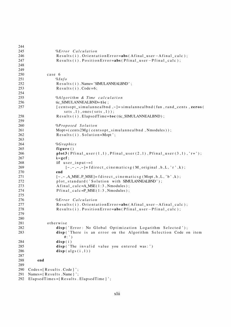
244245 %Error C a l c u l a t i o n246 R e s u l t s ( i ) . O r i e n t a t i o n E r r o r =abs ( A f i n a l _ u s e r−A f i n a l _ c a l c ) ;247 R e s u l t s ( i ) . P o s i t i o n E r r o r =abs ( P f i n a l _ u s e r−P f i n a l _ c a l c ) ;248249250 c a s e 6251 %I n f o252 R e s u l t s ( i ) . Name= ’SIMULANNEALBND’ ;253 R e s u l t s ( i ) . Code =6;254255 %A l g o r i t h m & Time c a l c u l a t i o n256 tic_SIMULANNEALBND= t i c ;257 [ c e n t s o p t _ s i m u l a n n e a l b n d , ~ ] = s i m u l a n n e a l b n d ( fun , r a n d _ c e n t s , z e r o s (

s e t s , 1 ) , ones ( s e t s , 1 ) ) ;258 R e s u l t s ( i ) . E lapsedTime = t o c ( tic_SIMULANNEALBND ) ;259260 %Proposed S o l u t i o n261 Mopt =( cents2Mg ( c e n t s o p t _ s i m u l a n n e a l b n d , Nmodules ) ) ;262 R e s u l t s ( i ) . S o l u t i o n =Mopt ’ ;263264 %Graph ics265 f i g u r e ( )266 p l o t 3 ( P f i n a l _ u s e r ( 1 , 1 ) , P f i n a l _ u s e r ( 2 , 1 ) , P f i n a l _ u s e r ( 3 , 1 ) , ’ r + ’ ) ;267 k= g c f ;268 i f u s e r _ i n p u t ~=1269 [ ~ , ~ , ~ , ~ ] = f d i r e c t _ c i n e m a t i c s g ( M_or ig ina l , h , L , ’ r ’ , k ) ;270 end271 [ ~ , ~ ,A_MSE, P_MSE]= f d i r e c t _ c i n e m a t i c s g ( Mopt , h , L , ’ b ’ , k ) ;272 p l o t _ s t a n d a r d ( ’ S o l u t i o n wi th SIMULANNEALBND’ ) ;273 A f i n a l _ c a l c =A_MSE( 1 : 3 , Nmodules ) ;274 P f i n a l _ c a l c =P_MSE ( 1 : 3 , Nmodules ) ;275276 %Error C a l c u l a t i o n277 R e s u l t s ( i ) . O r i e n t a t i o n E r r o r =abs ( A f i n a l _ u s e r−A f i n a l _ c a l c ) ;278 R e s u l t s ( i ) . P o s i t i o n E r r o r =abs ( P f i n a l _ u s e r−P f i n a l _ c a l c ) ;279280281 o t h e r w i s e282 di sp ( ’ E r r o r : No G lob a l O p t i m i z a t i o n Logar i thm S e l e c t e d ’ ) ;283 di sp ( ’ There i s an e r r o r on t h e Algo r i t hm S e l e c t i o n Code on i t em

# : ’ )284 di sp ( i )285 di sp ( ’ The i n v a l i d v a l u e you e n t e r e d was : ’ )286 di sp ( a l g s ( i , 1 ) )287288 end289290 Codes =[ R e s u l t s . Code ] ’ ;291 Names={ R e s u l t s . Name } ’ ;292 ElapsedTimes =[ R e s u l t s . E lapsedTime ] ’ ;

xlii

293 S o l u t i o n s =[ R e s u l t s . S o l u t i o n ] ;294 P o s i t i o n E r r o r s =[ R e s u l t s . P o s i t i o n E r r o r ] ;295 O r i e n t a t i o n E r r o r s =[ R e s u l t s . O r i e n t a t i o n E r r o r ] ;296 PPTimes =[ Codes ElapsedTimes ] ;

xliii

Plot Plate

1 f u n c t i o n p l o t _ p l a t e ( P u n i t , L , c o l o r e s )2 %%F u n c t i o n t o p l o t t h e squares ’ l i n e o f each module34 N= P u n i t ( 1 : 3 , 1 ) ;5 O= P u n i t ( 1 : 3 , 2 ) ;6 A= P u n i t ( 1 : 3 , 3 ) ;7 P= P u n i t ( 1 : 3 , 4 ) ;8 d i s t =L ∗ ( 2 ^ ( 1 / 2 ) / 2 ) ;9

10 NO=N+O;11 NO=NO/ norm (NO) ;1213 %V e r t i x c a l c u l a t i o n14 P o i n t 1 =P+ r o t _ a n y (NO’ , pi / 2 ,A’ ) ∗ d i s t ;15 P o i n t 2 =P+ r o t _ a n y (NO’ , 0 ,A’ ) ∗ d i s t ;16 P o i n t 3 =P+ r o t _ a n y (NO’ ,− pi / 2 ,A’ ) ∗ d i s t ;17 P o i n t 4 =P+ r o t _ a n y (NO’ , pi , A’ ) ∗ d i s t ;1819 %Line P l o t t i n g be tween v e r t i x20 C=[ P o i n t 1 P o i n t 2 P o i n t 3 P o i n t 4 P o i n t 1 ] ’ ;21 H= l i n e (C ( : , 1 ) , C ( : , 2 ) , C ( : , 3 ) ) ;22 s e t (H, ’ c o l o r ’ , c o l o r e s ) ;2324 end

xliv

Plot Point

1 f u n c t i o n p l o t _ p o i n t ( P0 , P u n i t , c o l o r e s )2 %%F u n c t i o n t o p l o t t h e modules ’ c e n t r a l p o i n t and ’ s p i n e ’34 H1= p l o t 3 ( P u n i t ( 1 , 4 ) , P u n i t ( 2 , 4 ) , P u n i t ( 3 , 4 ) ) ; %P l o t t i n g each p o i n t56 vx =[ P0 ( 1 , 4 ) P u n i t ( 1 , 4 ) ] ;7 vy =[ P0 ( 2 , 4 ) P u n i t ( 2 , 4 ) ] ;8 vz =[ P0 ( 3 , 4 ) P u n i t ( 3 , 4 ) ] ;9

10 H2= l i n e ( vx , vy , vz ) ;1112 s e t ( H1 , ’ c o l o r ’ , c o l o r e s ) ;13 s e t ( H2 , ’ c o l o r ’ , c o l o r e s ) ;141516 end

xlv

Plot Standard

1 f u n c t i o n p l o t _ s t a n d a r d ( t i t u l o )2 %%F u n c t i o n t o s t a n d a r i z e g r a p h i c s34 t i t l e ( t i t u l o )5 x l a b e l ( ’X [m] ’ )6 y l a b e l ( ’Y [m] ’ )7 z l a b e l ( ’Z [m] ’ )8 gr id on9

10 end

xlvi

Rot Any

1 f u n c t i o n T _ r o t _ t r a n s = r o t _ a n y ( vec t , r o t _ a n g l e , r o t _ a x i s _ v e c t )2 %%F u n c t i o n t o c a l c u l a t e t h e r e s u l t o f r o t a t i n g a v e c t o r ’ v e c t ’ around a

r o t a t i o n a x i s d e s c r i b e d by ’ r o t _ a x i s _ v e c t ’ ove r a c e r t a i n r o t a t i o n a n g l e’ r o t _ a n g l e ’

34 T _ r o t _ t r a n s 1 = z e r o s ( 3 ) ;56 u n i t _ r o t _ a x i s _ v e c t = r o t _ a x i s _ v e c t / ( norm ( r o t _ a x i s _ v e c t ) ) ;789 u= u n i t _ r o t _ a x i s _ v e c t ( 1 , 1 ) ;

10 v= u n i t _ r o t _ a x i s _ v e c t ( 1 , 2 ) ;11 w= u n i t _ r o t _ a x i s _ v e c t ( 1 , 3 ) ;1213 u2=u ^ 2 ;14 v2=v ^ 2 ;15 w2=w^ 2 ;16 c= cos ( r o t _ a n g l e ) ;17 s= s i n ( r o t _ a n g l e ) ;1819 T _ r o t _ t r a n s 1 ( 1 , 1 ) =u2 + ( v2 + w2 ) ∗c ;20 T _ r o t _ t r a n s 1 ( 1 , 2 ) =u∗v∗(1−c ) − w∗ s ;21 T _ r o t _ t r a n s 1 ( 1 , 3 ) =u∗w∗(1−c ) + v∗ s ;22 T _ r o t _ t r a n s 1 ( 2 , 1 ) =u∗v∗(1−c ) + w∗ s ;23 T _ r o t _ t r a n s 1 ( 2 , 2 ) =v2 + ( u2+w2 ) ∗c ;24 T _ r o t _ t r a n s 1 ( 2 , 3 ) =v∗w∗(1−c ) − u∗ s ;25 T _ r o t _ t r a n s 1 ( 3 , 1 ) =u∗w∗(1−c ) − v∗ s ;26 T _ r o t _ t r a n s 1 ( 3 , 2 ) =v∗w∗(1−c ) +u∗ s ;27 T _ r o t _ t r a n s 1 ( 3 , 3 ) =w2 + ( u2+v2 ) ∗c ;2829 T _ r o t _ t r a n s = T _ r o t _ t r a n s 1 ∗ vec t ’ ;303132 end

xlvii

Unit Vector Mat

1 f u n c t i o n [ U_mat ]= u n i t _ v e c t o r _ m a t ( P )2 %%F u n c t i o n t o n o r m a l i z e NOA v e c t o r s i n m a t r i x ’P ’34 U_mat= z e r o s ( 4 ) ;5 U_mat ( 1 : 4 , 4 ) =P ( 1 : 4 , 4 ) ;67 f o r i = 1 : 1 : 38 U_mat ( 1 : 3 , i ) =P ( 1 : 3 , i ) / ( norm ( P ( 1 : 3 , i ) ) ) ;9 end

xlviii

Inverse Kinematics of a 10 DOF Modular Hyper-Redundant ...

Documents

Transcript of Inverse Kinematics of a 10 DOF Modular Hyper-Redundant ...