
INVENTORY MANAGEMENT THROUGH VENDOR MANAGED INVENTORY · PDF fileinventory management through...
80
INVENTORY MANAGEMENT THROUGH VENDOR MANAGED INVENTORY IN A SUPPLY CHAIN WITH STOCHASTIC DEMAND A THESIS SUBMITTED TO THE GRADUATE SCHOOL OF NATURAL AND APPLIED SCIENCES OF MIDDLE EAST TECHNICAL UNIVERSITY BY HÜRDOĞAN GÜNEġ IN PARTIAL FULFILLMENT OF THE REQUIREMENTS FOR THE DEGREE OF MASTER OF SCIENCE IN INDUSTRIAL ENGINEERING SEPTEMBER 2010
Transcript of INVENTORY MANAGEMENT THROUGH VENDOR MANAGED INVENTORY · PDF fileinventory management through...
INVENTORY MANAGEMENT THROUGH VENDOR MANAGED
INVENTORY IN A SUPPLY CHAIN
WITH STOCHASTIC DEMAND
A THESIS SUBMITTED TO
THE GRADUATE SCHOOL OF NATURAL AND APPLIED SCIENCES
OF
MIDDLE EAST TECHNICAL UNIVERSITY
BY
HÜRDOĞAN GÜNEġ
IN PARTIAL FULFILLMENT OF THE REQUIREMENTS
FOR
THE DEGREE OF MASTER OF SCIENCE
IN
INDUSTRIAL ENGINEERING
SEPTEMBER 2010
Approval of the thesis
INVENTORY MANAGEMENT THROUGH VENDOR MANAGED
INVENTORY IN A SUPPLY CHAIN
WITH STOCHASTIC DEMAND
Submitted by HÜRDOĞAN GÜNEŞ in partial fulfillment of the requirements for
the degree of Master of Science in Industrial Engineering Department, Middle
East Technical University by,
Prof. Dr. Canan ÖZGEN
Dean, Graduate School of Natural and Applied Sciences ___________
Prof. Dr. Nur Evin ÖZDEMĠREL
Head of Department, Industrial Engineering ___________
Assist. Prof. Dr. Seçil SAVAġANERĠL
Supervisor, Industrial Engineering Dept., METU ___________
Assist. Prof. Dr. Zeynep Pelin BAYINDIR
Co-Supervisor, Industrial Engineering Dept., METU ___________
Examining Committee Members:
Assoc. Prof. Dr. Sedef MERAL
Industrial Engineering Dept., METU ___________
Assist. Prof. Dr. Seçil SAVAġANERĠL
Industrial Engineering Dept., METU ___________
Assist. Prof. Dr. Zeynep Pelin BAYINDIR
Industrial Engineering Dept., METU ___________
Assist. Prof. Dr. Ferda Can ÇETĠNKAYA
Industrial Engineering Dept., Çankaya University ___________
Dr. Benhür SATIR
Industrial Engineering Dept., Çankaya University ___________
Date: 17.09.2010
iii
I hereby declare that all information in this document has been obtained and
presented in accordance with academic rules and ethical conduct. I also declare
that, as required by these rules and conduct, I have fully cited and referenced
all material and results that are not original to this work.
Name, Last name: Hürdoğan GÜNEġ
Signature :
iv
ABSTRACT
INVENTORY MANAGEMENT THROUGH VENDOR
MANAGED INVENTORY IN A SUPPLY CHAIN WITH
STOCHASTIC DEMAND
GÜNEġ, Hürdoğan
M.S., Department of Industrial Engineering
Supervisor : Assist. Prof. Dr. Seçil SAVAġANERĠL
Co-Supervisor : Assist. Prof. Dr. Zeynep Pelin BAYINDIR
September 2010, 68 pages
Vendor Managed Inventory (VMI) is a business practice in which vendors monitor
their customers‟ inventories, and decide when and how much inventory should be
replenished. VMI has attracted a lot of attention due to its benefits. In this study, we
analyze the benefits of VMI in a supply chain consisting of a single retailer and a
single capacitated supplier under stochastic demand. We propose a VMI setting and
compare the vendor managed system with the traditional system to quantify the
benefits of VMI. In our proposed VMI system, the retailer shares the inventory level
information with the supplier, which is not available in traditional system; and the
supplier is responsible to keep the retailer‟s inventory level between the specified
minimum and maximum values, called (z,Z) levels, set by a contract. We examine
the benefits of such a VMI system for each member and for the overall chain; and
analyze the effects of system parameters on these benefits. The performance of VMI
in coordinating the overall chain is examined under different system parameters.
Keywords: Vendor Managed Inventory, Supply Chain Coordination
v
ÖZ
BİR TEDARİK ZİNCİRİ İÇİN STOKASTİK TALEP ALTINDA
TEDARİKÇİ KONTROLÜ İLE ENVANTER YÖNETİMİ
GÜNEġ, Hürdoğan
Yüksek Lisans, Endüstri Mühendisliği Bölümü
Tez Yöneticisi : Yrd. Doç. Dr. Seçil SAVAġANERĠL
Ortak Tez Yöneticisi : Yrd. Doç. Dr. Zeynep Pelin BAYINDIR
Eylül 2010, 68 sayfa
Tedarikçi Kontrollü Envanter Yönetimi (VMI), tedarikçilerin müĢterilerinin
envanterini kontrol ettiği, ne zaman ve ne miktarda yeniden doldurulacağına karar
verdiği bir iĢ yöntemidir. VMI, sağladığı faydalar nedeniyle oldukça dikkat
çekmektedir. Bu çalıĢmada, VMI uygulamasının stokastik talep altında bir
perakendeci ve bir tedarikçiden oluĢan tedarik zincirindeki faydaları incelenmiĢtir.
Bir VMI uygulaması tasarlanmıĢ ve tedarikçi kontrollü sistemle geleneksel sistem
kıyaslanarak VMI uygulamasının faydaları niceliksel olarak gösterilmiĢtir.
Tasarladığımız VMI uygulamasında perakendeci, geleneksel sistemde geçerli
olmayan bir Ģekilde stok seviyesine dair bilgileri tedarikçisiyle paylaĢmakla;
tedarikçi ise perakendecinin stok seviyesini aralarındaki sözleĢmece belirlenen ve
(z,Z) seviyesi olarak adlandırılan minimum ve maksimum seviyeler arasında
tutmakla yükümlüdür. Bu Ģekilde tasarlanan bir VMI sisteminin faydaları tedarik
zincirinin her bir üyesi ve zincirin bütünü için incelenmiĢ, sistem parametrelerinin bu
faydalara etkileri analiz edilmiĢtir. VMI uygulamasının tedarik zincirini bütünüyle
koordine edebilme performansı farklı parametreler altında incelenmiĢtir.
Anahtar Kelimeler: Tedarikçi Kontrollü Envanter Yönetimi, Tedarik Zinciri
Koordinasyonu

vi
Rüzgar’a
vii
ACKNOWLEDGEMENTS
I would like to express my most sincere gratitude to my advisors, Assist. Prof.
Dr. Seçil SavaĢaneril and Assist. Prof. Dr. Zeynep Pelin Bayındır for all the trust,
endless patience and endurance that they showed during my graduate study.
I am grateful to my dear friends Volkan, Akbay, Tufan and Ümit Baba for
their sincere friendship and morale support.
I thank my family for being there when I needed most. They are the most
valuable for me.
viii
TABLE OF CONTENTS
ABSTRACT ............................................................................................................................ iv
ÖZ ............................................................................................................................................ v
ACKNOWLEDGEMENTS ................................................................................................... vii
TABLE OF CONTENTS ...................................................................................................... viii
LIST OF FIGURES ................................................................................................................. x
LIST OF TABLES ................................................................................................................. xii
CHAPTER 1 ............................................................................................................................ 1
INTRODUCTION ................................................................................................................... 1
CHAPTER 2 ............................................................................................................................ 4
LITERATURE REVIEW ........................................................................................................ 4
CHAPTER 3 ............................................................................................................................ 9
MODEL ................................................................................................................................... 9
3.1 TRADITIONAL SETTING ................................................................................... 12
3.1.1 The Model For The Retailer ........................................................................... 12
3.1.2 The Model For The Supplier .......................................................................... 16
3.2 VMI SETTING ...................................................................................................... 22
3.3 CENTRALIZED SETTING .................................................................................. 29
CHAPTER 4 .......................................................................................................................... 31
COMPUTATIONAL STUDY ............................................................................................... 31
4.1 Benefit of VMI on Supplier‟s Profit: ..................................................................... 32
4.1.1 Effect of Demand Variation: .......................................................................... 33
4.1.2 Effect of Capacity .......................................................................................... 35
4.1.3 Effect of Retail and Wholesale Price ............................................................. 37
4.2 Benefit of VMI on Retailer‟s Profit ....................................................................... 39
4.2.1 Effect of Demand Variation ........................................................................... 39
4.2.2 Effect of Retail and Wholesale Price ............................................................. 40
4.3 The Performance of VMI and Benefit on Supply Chain Profit ............................. 42
4.3.1 Effect of Demand Variation ........................................................................... 43
4.3.2 Effect of Capacity ......................................................................................... 45
ix
4.3.3 Effect of Order Cost Sharing ......................................................................... 46
4.3.4 Effect of Retail and Wholesale Price ............................................................. 48
CHAPTER 5 .......................................................................................................................... 50
CONCLUSION ...................................................................................................................... 50
REFERENCES ...................................................................................................................... 52
APPENDIX A ........................................................................................................................ 54
List of Notation ...................................................................................................................... 54
APPENDIX B ........................................................................................................................ 57
The Algorithm For Generating P(t,Q) – A Numerical Example ........................................... 57
APPENDIX C ........................................................................................................................ 60
Computational Study – The Supplier‟s Profit in Traditional and VMI Setting ..................... 60
APPENDIX D ........................................................................................................................ 63
Computational Study – The Retailer‟s Profit Under The Traditional and The VMI Setting . 63
APPENDIX E ........................................................................................................................ 66
Computational Study – Total Supply Chain Profit Under The Traditional and The VMI
Settings ................................................................................................................................... 66
x
LIST OF FIGURES
Figure 3. 1: Traditional Setting ................................................................................................ 9
Figure 3. 2: VMI Setting ........................................................................................................ 10
Figure 3. 3: Centralized Setting ............................................................................................. 10
Figure 4. 1: Profit of The Supplier vs Coefficient of Variation (cvd) Under Traditional and
VMI Setting (C = 15; pr = 15; αs = 0.25)................................................................................ 34
Figure 4. 2: Benefit of VMI on Supplier‟s Profit vs Coefficient of Variation (C = 15;
pr = 15; αs = 0.25)................................................................................................................... 35
Figure 4. 3: Benefits of VMI on Supplier‟s Profit vs Capacity (αs = 0.25)............................ 36
Figure 4. 4: Profit of The Supplier vs Retail Price (pr) Under Traditional and VMI Settings
(C = 15; cvd = 0.522; αs = 0.25) ............................................................................................. 37
Figure 4. 5: Benefit of VMI on Supplier‟s Profit vs Retail Price (C = 15; αs = 0.25) ............ 38
Figure 4. 6: Profit of The Retailer vs Coefficient of Variation (cvd) Under Traditional and
VMI Settings (C = 15; pr = 15; αs = 0.25) .............................................................................. 39
Figure 4. 7: Benefit of VMI on Retailer‟s Profit vs Coefficient of Variation (C = 15;
αs = 0.25) ................................................................................................................................ 40
Figure 4. 8: Profit of The Retailer vs Retail Price (pr) Under Traditional and VMI Settings
(C = 15; αs = 0.25; cvd = 0.522) ............................................................................................. 41
Figure 4. 9: Benefit of VMI on Retailer‟s Profit vs Retail Price (C = 15; αs = 0.25) ............ 41
Figure 4. 10: Profit of The Supply Chain vs Coefficient of Variation (cvd) (C = 15; pr = 15;
w = 8; αs = 0.25) ..................................................................................................................... 43
Figure 4. 11: Benefit of VMI on Supply Chain Profit vs Coefficient of Variation (C = 15;
pr = 15; w = 8; αs = 0.25)........................................................................................................ 44
Figure 4. 12: Performance of VMI vs Coefficient of Variation (C = 15; pr = 15; αs = 0.25) 44
Figure 4. 13: Benefit of VMI on Supply Chain Profit vs Capacity (pr = 15; αs = 0.25) ........ 45
Figure 4. 14: Performance of VMI vs Capacity (αs = 0.25) ................................................... 46

xi
Figure 4. 15: Benefit of VMI on Supply Chain Profit vs Order Cost Sharing Ratio (αs) ...... 47
Figure 4. 16: Performance of VMI vs Order Cost Sharing Ratio (αs) .................................... 47
Figure 4. 17: Benefit of VMI on Supply Chain Profit vs Retail Price (C = 15; αs = 0.25) .... 48
Figure 4. 18: Performance of VMI vs Retail Price (C = 15; αs = 0.25) ................................. 49
xii
LIST OF TABLES
Table 3. 1: Problem Environment For The Traditional, VMI and Centralized Settings ........ 11
Table 4. 1: Parameters and Their Values Used in Computational Study ............................... 31
Table 4. 2: Cost Parameters and Fixed Values Used in Computational Study ...................... 32
Table C. 1: Profit of The Supplier Under The Traditional and VMI Settings For Each
Parameter Set (αs = 0.25) ....................................................................................................... 60
Table C. 2: Profit of The Supplier Under The Traditional and VMI Settings For Each
Parameter Set (αs = 0.50) ....................................................................................................... 61
Table C. 3: Profit of The Supplier Under The Traditional and VMI Settings For Each
Parameter Set (αs = 0.75) ....................................................................................................... 62
Table D. 1: Profit of The Retailer Under The Traditional and VMI Settings For Each
Parameter Set (αs = 0.25) ....................................................................................................... 63
Table D. 2: Profit of The Retailer Under The Traditional and VMI Settings For Each
Parameter Set (αs = 0.50) ....................................................................................................... 64
Table D. 3: Profit of The Retailer Under The Traditional and VMI Settings For Each
Parameter Set (αs = 0.75) ....................................................................................................... 65
Table E. 1: Supply Chain Profit Under The Traditional and VMI Settings For Each
Parameter Set (αs = 0.25) ....................................................................................................... 66
Table E. 2: Supply Chain Profit Under The Traditional and VMI Settings For Each
Parameter Set (αs = 0.50) ....................................................................................................... 67
Table E. 3: Supply Chain Profit Under The Traditional and VMI Settings For Each
Parameter Set (αs = 0.75) ....................................................................................................... 68
1
CHAPTER 1
INTRODUCTION
A company which is involved in supply chain operations should perform the
processes of sourcing of raw materials and components, producing and dispatching
the finished products to customers. The main concern of each company is to
minimize the operational cost and to maximize profit.
Although being a part of the supply chain, a firm still focuses on optimizing
its own costs or profits, because the decisions concerning production and
replenishment are made separately and independently by the members of that chain.
However, a supply chain implies the interaction of its members, even when they have
different operational goals. Technological advancements and the realization that each
company is a part of one or more supply chains that dictate its performance and
effectiveness have resulted to the adoption of cooperative strategies through
information sharing and contracting.
“In fact, the performance of a supply chain depends not only on how well
each member manages its operational processes, but also on how well the members
coordinate their decisions” (Achabal 2000). For this reason, coordinating the
decisions is significant in a supply chain, even each member of the chain has
different own operational goals.
Vendor Managed Inventory (VMI) is a popular and widely discussed
partnership between the members of the supply chain which was popularized in the
late 1980‟s by Wal-Mart and Procter & Gamble and resulted in significant benefits.
2
After this successful application, many other firms, such as Campbell Soup
Company, Barilla and Intel, have also implemented VMI in their supply chains.
VMI is an inter-organizational relationship that the retailer shares the
information of end-item demand and the inventory level information with the
supplier and the supplier uses this information for better management of the retailer‟s
inventory. “Although it depends on the form of the agreement, the benefits of VMI
generally include improved service level and reduced supply chain costs, reduced
customer-demand uncertainty, reduced stock-outs and stock-out frequency, and
reduced bullwhip effect” (Waller, Johnson and Davis 1999).
In this study, we model a supply chain which is composed of a single retailer
(he) and a single capacitated supplier (she). We define a traditional system under
which the retailer manages his own inventory, and then introduce a system with VMI
agreement. We analyze the benefits of VMI for the retailer, for the supplier and for
the total chain. The retailer faces stochastic customer demand at each period and in
the traditional setting, he periodically places orders to the supplier. In the traditional
setting, the supplier is assumed to know the end-demand distribution and the
inventory policy of the retailer with its parameter values. She infers the probability
distribution of the retailer‟s demand by using this information. The information of
the retailer‟s inventory level is not available to the supplier in the traditional system,
although she has full information in the VMI system. Availability of information in
traditional and VMI systems is similar to partial and full information models defined
and analyzed in Gavirneni, Kapuscinski and Tayur (1999).
In a VMI system, if the supplier‟s control were unlimited, then without some
form of penalty costs at the supplier, it would be optimal for the supplier to dispatch
large volumes of inventory to the retailer. In real life systems, however, the supplier
is limited in her replenishments and in other operational decisions under VMI by an
agreement or contract between the participant firms (Fry, Kapuscinski and Olsen
2001). The implementation and details of VMI contracts differ from company to
company and may specify various parameters to control the replenishments of the
supplier, such as customer service level, allocated storage or shelf space (Fry,
3
Kapuscinski and Olsen (2001) provides the examples of VMI agreements used in
practice). In our study, under the VMI setting, the supplier is expected (or forced) to
keep the retailer‟s inventory level between the specified two values, which are
denoted as (z,Z) levels. These specified levels should satisfy that each player in the
chain is never worse off under the VMI setting when compared to the traditional
case. In the new system, the fixed ordering cost of the retailer (transportation cost) is
also shared between the retailer and the supplier in different ratios, although it is
fully incurred by the retailer in traditional setting.
We aim to examine the benefits of VMI for the retailer, for the supplier and
for the overall chain in this study and we analyze how these benefits under VMI
setting change with system parameters.
Depending on the form of the agreement between the supplier and the retailer,
the supply chain under VMI may be very close to a centralized system, that is, it may
operate on conditions which are very close to optimal. One of our aims is to measure
the performance of such an agreement to coordinate the chain by comparing its
benefit on total supply chain by a centralized system.
The remainder of the study is organized as follows. A literature review related
to the VMI systems is provided in Chapter 2. In Chapter 3, we present the supply
chain environments and the models for the traditional, VMI and the centralized
settings. We present our computational study results in Chapter 4. The benefits of
VMI for the supplier, for the retailer and for the overall supply chain under different
system parameters are analyzed in this chapter. In Chapter 5, we conclude the study
by stating a summary of our work and by discussing on the further study issues.
4
CHAPTER 2
LITERATURE REVIEW
Vendor Managed Inventory (VMI) systems have been studied from many
aspects. A considerable amount of researches in this literature addresses the benefits
of information sharing in a supply chain. Benefit of VMI as a supply chain
coordinator is studied by many researchers. VMI contractual agreements are also
studied in the related literature.
Co-operative policies and information sharing are one of the focuses in VMI
research. There exist considerable amount of articles studying these issues.
Gavirneni, Kapuscinski and Tayur (1999) analyze the value of information in a
supply chain with single retailer and a single capacitated supplier. The authors study
the partial and the full information sharing and compare these to a traditional case of
no information. As a partial information sharing, the benefit of knowing he retailer‟s
inventory policy parameters, (s,S) policy, is examined. In complete information
sharing case, they examine the benefits of knowing the retailer‟s inventory level.
They found that the information sharing is most beneficial when the capacity is not
restrictive. Cachon and Fisher (2000) find only limited benefits to information
sharing. They analyze a supply chain which consists of multiple retailers and a single
supplier. The retailers order an integer number of batches and the supplier uses a
batch priority allocation process among these retailers. They conclude that the extra
benefit of demand information is limited for the supplier, since it is most valuable
just before an order is placed by the retailer. Aviv and Federgruen (1998) analyze
VMI from the perspective of information sharing. They find that information sharing
with VMI always provides more benefits than pure information sharing.
5
The incentive issues in VMI contractual agreements are also studied in VMI
literature. Fry, Kapuscinski and Olsen (2001) model a specific (z,Z)-type of VMI
agreement in a supply chain environment with a single manufacturer and a single
retailer with stochastic demand and compare the VMI system with a traditional case
under full information sharing. In this type of contract, the retailer sets the inventory
levels, z and Z, that represent the lowest and highest inventory levels, respectively.
The manufacturer should keep the retailer‟s inventory level between these specified
levels. The manufacturer follows a fixed production schedule, but can replenish the
retailer in any period and she incurs a penalty cost if she cannot keep the retailer‟s
inventory level between the specified levels. They make a comparison between the
VMI system and the traditional system with information sharing and find that VMI
can perform significantly better than the traditional case in many settings but can
perform worse in others. Their numerical analyses also show that when the
outsourcing cost and the demand variation is high, VMI performs close to a
centralized system.
VMI provides flexibility in delivery and in operational decisions. Several
studies focus on these benefits provided by the VMI agreements in a single supplier-
multiple retailer supply chain environments. “The flexibility may enable a supplier to
combine routes from multiple origins and delay stock assignments, consolidate
shipments to two or more customers, or postpone a decision on the quantity destined
for each of them” (Gumus 2006). Aviv and Federgruen (1998) study the effects of
information sharing under periodic inventory review in a supply chain with single
supplier and multiple retailer. They assume a VMI agreement that leads to a fully
centralized planning model where the supplier minimizes the system-wide total cost
of inventory holding and distribution. They construct the optimal policies for the
supplier and the retailers under VMI with information sharing and under information
sharing alone. They conclude that VMI provides more benefits than information
sharing alone. Cheung and Lee (2002) also study the flexibility of delivery to
multiple retailers offered by VMI in terms of shipment coordination and stock
balancing. Similarly, Çetinkaya and Lee (2000) analyze the synchronization of
inventory and dispatch decisions under VMI. They assume that under VMI, the
supplier can hold orders until a suitable shipment time, at which orders can be
6
economically consolidated. They derive the optimal policy under VMI and conclude
that shipment consolidation is beneficial if the outsourcing and holding costs are low.
Waller, Johnson and Davis (1999) studies the impacts of VMI under different levels
of demand variability. They demonstrate that a reduction in inventory is achieved in
VMI and this is the result of frequent reviews and shorter intervals between
replenishments. Kleywegt, Nori and Savelsbergh (2002) also study a single supplier-
multiple retailer supply chain environment in order to determine the optimal
distribution policy of a single product.
Supply chain coordination is another stream of research. A supply chain may
be very close to a centralized system depending on the performance of the VMI
agreement between the supplier and the retailer. The effects of VMI agreements to
the coordination of the supply chain is studied in the literature. Cachon (2001)
studies VMI in a supply chain with a single supplier-multiple retailers. He analyzes
various strategies with the aim of channel coordination. He employs game theory to
find the equilibrium for each member of the supply chain. Cachon (2001) remarks
that “VMI alone does not guarantee an optimal supply-chain solution; both the
vendor and retailers must also agree to make fixed transfer payments to participate in
the VMI contract, and then be willing to share the benefits.” Bernstein, Chen and
Federgruen (2006) study a partially centralized VMI model. For the supply chain a
replenishment strategy is determined. They find that when the demand rate is
constant and a single retailer retains the decision rights on pricing, the channel
coordination can be achieved. In their supply chain environment, the supplier incurs
holding costs of the retailer. Therefore, their system considers consignment inventory
with VMI. Dong and Xu (2002) analyze the different impacts of a VMI program on a
supply channel in terms of total chain cost and supplier‟s cost. The purchasing price
is set by the retailers in the contract; however the selling quantity is determined by
the supplier in their model. They find that total chain cost is reduced by VMI, but the
profit of the supplier could decrease under some certain conditions. They argue that
VMI is an effective strategy that can realize many of the benefits obtainable only in a
fully integrated supply channel. Narayanan and Raman (1997) and Fry, Kapuscinski
and Olsen (2001) also analyze VMI agreements under stochastic demand and discuss
centralization. One aim of our study is to analyze the benefits of the VMI agreement
7
on the total supply chain and to measure the performance of VMI in coordinating the
supply chain by comparing the supply chain profits under VMI setting with the
centralized system.
The VMI agreement may also specify a consignment stock, whereby the
retailer will not be invoiced until he sells the product to end customers. Several
research employ the consignment stock with VMI. Valentini and Zavanella (2003)
discuss the use of consignment stock by a manufacturer who manages the inventory
of her customer based on (s,S) policy. Their analysis and computational studies show
that consignment stock outperforms the usual inventory models. In a very recent
study, Zavanella and Zanoni (2009) examine a consignment stock system in a single
supplier-multiple retailers supply chain environment with discrete demand. They
offer an analytical model to analyze the benefits of consignment stock and to obtain
the optimal replenishment decisions both for the supplier and the retailers. They
show that according to the structure of the chain, the joint management of the
inventory gives modest or relevant rise to economic benefits. In our study, the
retailer is invoiced just after the replenishment. Therefore, our supply chain
environment does not represent a consignment system.
We study a periodic review inventory control problem in a supply chain with
a single retailer and a single supplier under stochastic demand. We propose a VMI
agreement and compare the VMI setting with the traditional case to quantify the
benefits of VMI. In our proposed VMI agreement, the retailer shares the inventory
level information with the supplier, which is not available in traditional system, and
the supplier is responsible to keep the retailer‟s inventory level between the
minimum and maximum levels set by the contract. We analyze the benefits of such
an agreement for each member and also for the supply chain. Furthermore, we aim to
measure the performance of the VMI agreement in coordinating the overall chain by
comparing it with the centralized system.
Our work is one of the few studies that consider a specific type of VMI
agreement and differs from the existing studies in the following aspects. (i) We
analyze the benefits VMI from the perspective of each member and the supply chain.
(ii) We utilize fixed cost sharing as the motivation for the retailer to join in a VMI
8
partnership. (iii) Apart from the benefits over the traditional system, we analyze the
performance of the vendor managed system in coordinating the supply chain. (iv)
Finally, we analyze how the system parameters affect the benefits of VMI system.
9
CHAPTER 3
MODEL
We consider a periodic review inventory control problem in a supply chain
which consists of a single retailer (he) and a single capacitated supplier (she). Our
aim is to model a particular type of Vendor Managed Inventory (VMI) agreement
between the supplier and the retailer, and to investigate the benefits provided by such
an agreement.
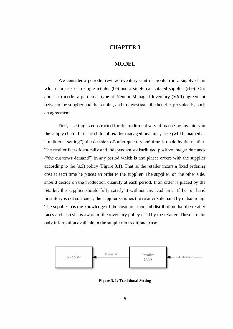
First, a setting is constructed for the traditional way of managing inventory in
the supply chain. In the traditional retailer-managed inventory case (will be named as
“traditional setting”), the decision of order quantity and time is made by the retailer.
The retailer faces identically and independently distributed positive integer demands
(“the customer demand”) in any period which is and places orders with the supplier
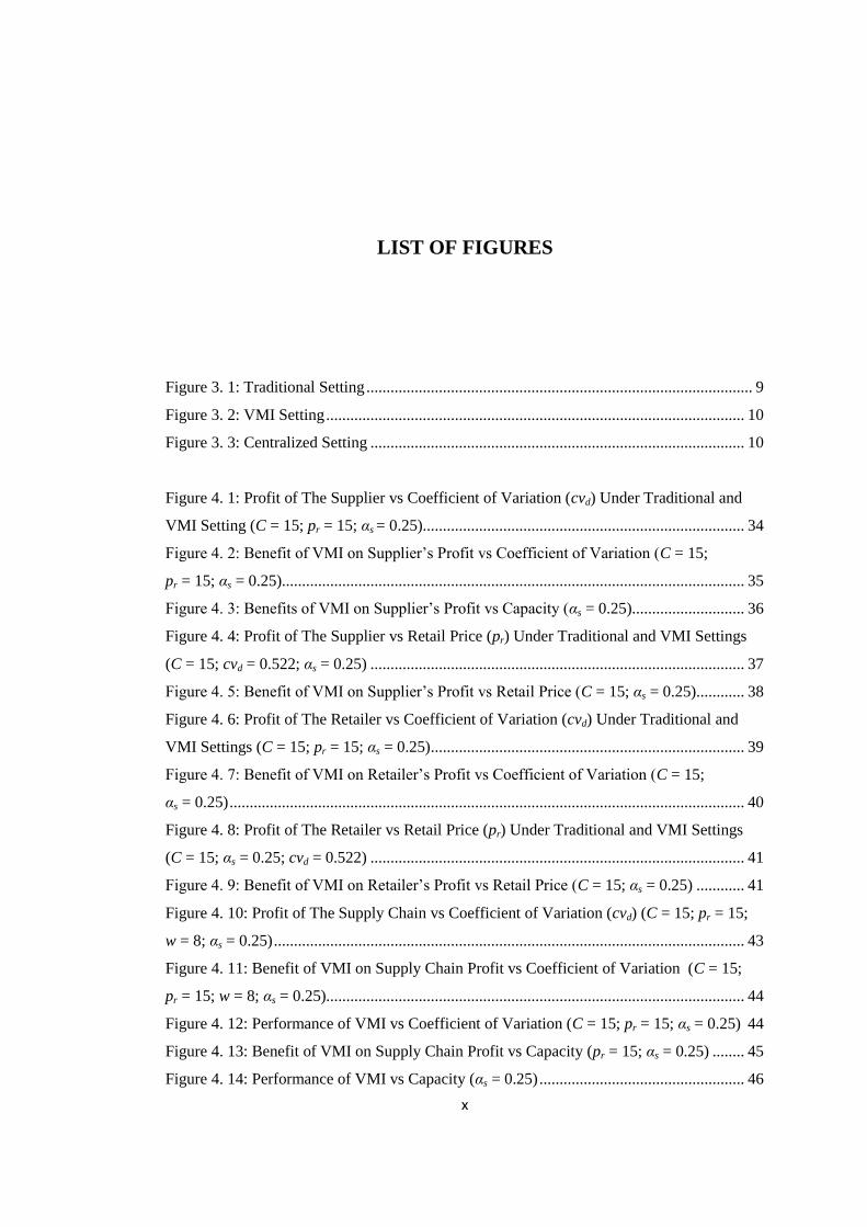
according to the (s,S) policy (Figure 3.1). That is, the retailer incurs a fixed ordering
cost at each time he places an order to the supplier. The supplier, on the other side,
should decide on the production quantity at each period. If an order is placed by the
retailer, the supplier should fully satisfy it without any lead time. If her on-hand
inventory is not sufficient, the supplier satisfies the retailer‟s demand by outsourcing.
The supplier has the knowledge of the customer demand distribution that the retailer
faces and also she is aware of the inventory policy used by the retailer. These are the
only information available to the supplier in traditional case.
Figure 3. 1: Traditional Setting
10
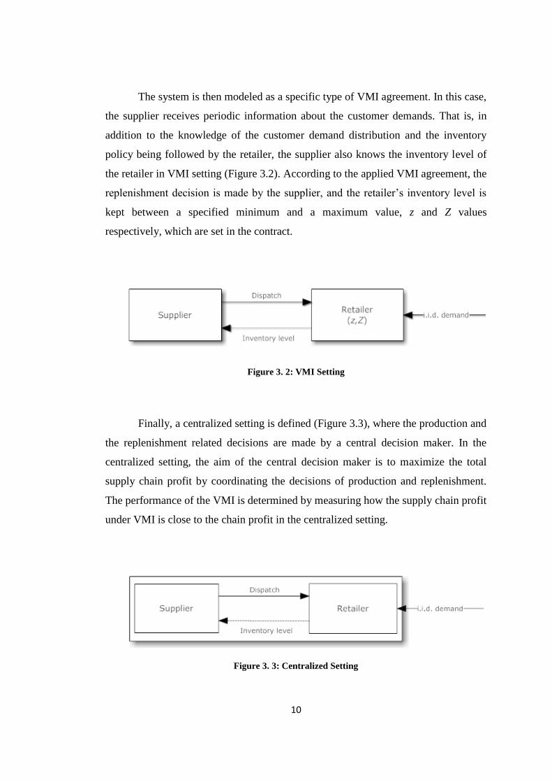
The system is then modeled as a specific type of VMI agreement. In this case,
the supplier receives periodic information about the customer demands. That is, in
addition to the knowledge of the customer demand distribution and the inventory
policy being followed by the retailer, the supplier also knows the inventory level of
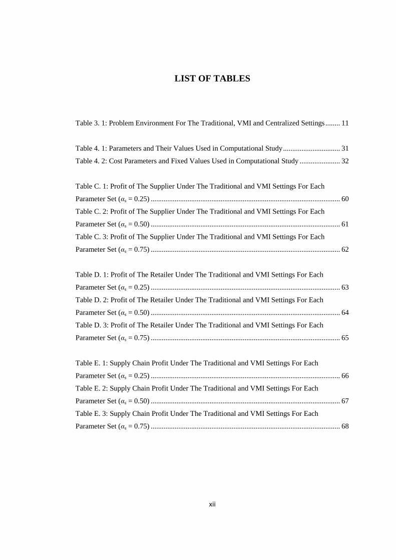
the retailer in VMI setting (Figure 3.2). According to the applied VMI agreement, the
replenishment decision is made by the supplier, and the retailer‟s inventory level is
kept between a specified minimum and a maximum value, z and Z values
respectively, which are set in the contract.
Figure 3. 2: VMI Setting
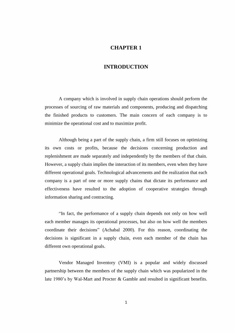
Finally, a centralized setting is defined (Figure 3.3), where the production and
the replenishment related decisions are made by a central decision maker. In the
centralized setting, the aim of the central decision maker is to maximize the total
supply chain profit by coordinating the decisions of production and replenishment.
The performance of the VMI is determined by measuring how the supply chain profit
under VMI is close to the chain profit in the centralized setting.
Figure 3. 3: Centralized Setting
11
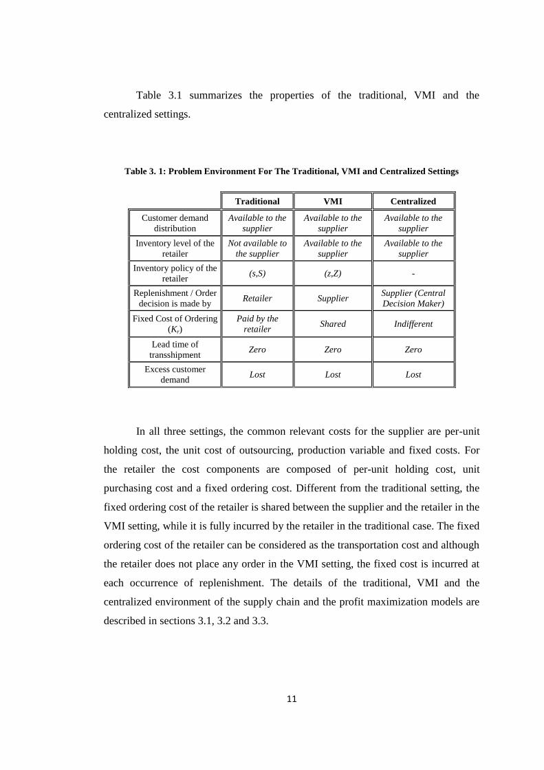
Table 3.1 summarizes the properties of the traditional, VMI and the
centralized settings.
Table 3. 1: Problem Environment For The Traditional, VMI and Centralized Settings
In all three settings, the common relevant costs for the supplier are per-unit
holding cost, the unit cost of outsourcing, production variable and fixed costs. For
the retailer the cost components are composed of per-unit holding cost, unit
purchasing cost and a fixed ordering cost. Different from the traditional setting, the
fixed ordering cost of the retailer is shared between the supplier and the retailer in the
VMI setting, while it is fully incurred by the retailer in the traditional case. The fixed
ordering cost of the retailer can be considered as the transportation cost and although
the retailer does not place any order in the VMI setting, the fixed cost is incurred at
each occurrence of replenishment. The details of the traditional, VMI and the
centralized environment of the supply chain and the profit maximization models are
described in sections 3.1, 3.2 and 3.3.
Traditional VMI Centralized
Customer demand
distribution
Available to the
supplier
Available to the
supplier
Available to the
supplier
Inventory level of the
retailer
Not available to
the supplier
Available to the
supplier
Available to the
supplier
Inventory policy of the
retailer (s,S) (z,Z) -
Replenishment / Order
decision is made by Retailer Supplier
Supplier (Central
Decision Maker)
Fixed Cost of Ordering
(Kr)
Paid by the
retailer Shared Indifferent
Lead time of
transshipment Zero Zero Zero
Excess customer
demand Lost Lost Lost
12
3.1 TRADITIONAL SETTING
In traditional way of managing inventory, there is no agreement or contract
between the supplier and the retailer. That is, there is no shared information about the
inventory level of the retailer. The retailer manages his own inventory, decides on the
replenishment time and quantity by himself. On the other hand, the supplier should
decide on the optimal production quantity in order to satisfy the retailer‟s demand
while maximizing her own profit. The sequence of events in traditional setting is as
follows: (1) First, the supplier decides how much to produce for the period. (2)
Customer demand occurs at the retailer and he satisfies the demand either fully or
partially (unsatisfied demand is lost). After satisfying the demand, he reviews his
inventory level and if required, places an order with the supplier. (3) The supplier
ships the demanded quantity to the retailer with a negligible lead time at the end of
the period. If her on-hand inventory is not sufficient to fully satisfy the retailer‟s
demand, then she does outsourcing. (4) Costs are incurred for the period.
The problem environments both for the retailer and the supplier in traditional
setting are evaluated separately and discussed in detail in sections 3.1.1 and 3.1.2.
Although the notation is described within the text when necessary, a full list of the
notation is provided in Appendix A.
3.1.1 The Model For The Retailer
In traditional setting the retailer manages his own inventory and focuses on
maximizing his profit by optimizing the ordering decisions.
The retailer faces stochastic demand and periodically places order to the
supplier. At the beginning of each period, the retailer checks his inventory level (Ir)
and decides on the order quantity (q). When he places an order, the supplier makes
the replenishment with a negligible lead time, and the retailer gets the exact quantity
of order each time. That is, the supplier fully satisfies the retailer‟s demand and
13
backorders are not allowed. After the replenishment, the retailer faces an integer
demand (customer demand). If the customer demand exceeds the retailer‟s on-hand
inventory, then it is assumed that the excess demand is lost. Since the ordered
quantity is fully dispatched to the retailer within the same period and the excess
demand of the customer is not backlogged, the inventory level of the retailer at the
beginning of the next period (Ir') is independent of the previous order decisions and
previous customer demands. The system represents a Markov chain with these
properties and the profit maximization problem of the retailer is modeled as a
Markov Decision Process (MDP).
The inventory level of the retailer at the beginning of each period, Ir,
represents the state of the system. At each state, the retailer decides on the order
quantity, q, and places order to the supplier, which represents the action. So, the state
space E and the action set A is composed of Ir and q values respectively, where Ir ≥ 0
and q ≥ 0.
If the system is in state Ir and the retailer places q units of order, then the
retailer‟s inventory level after the replenishment increases to Ir + q units. When D
units of customer demand occurs, then the retailer starts to the next period with Ir'
units of item with a probability of P(Ir'│Ir,q). The new state of the system, Ir', will be
equal to max (Ir + q –D, 0). The transition probability, P(Ir'│Ir,q), is expressed as;
P(Ir + q – Ir') when Ir' > 0;
when Ir' = 0;
where P(D) is the probability that the customer demand is equal to D units
(D>0).
The cost components for the retailer at each period are composed of per-unit
holding cost, unit purchasing cost and a fixed ordering cost. In order to express the
cost and revenue functions, the following notations are used:
: purchasing cost (includes fixed and variable cost) of the retailer
when the system is in state Ir E and decision q A is made.
P(Ir'│Ir,q) =
14
: expected inventory holding cost of the retailer if the system is in
state Ir E and decision q A is made.
: expected revenue of the retailer if the system is in state Ir E and
decision q A is made.
: expected profit of the retailer if system is in state Ir E and decision
q A is made
pr : unit selling price of the retailer (retail price)
w : unit selling price of the supplier (wholesale price)
hr : unit holding cost/period for the retailer
Kr : fixed ordering cost of the retailer
The retailer incurs a fixed ordering cost at each time he places an order to the
supplier. So, the purchasing cost of the retailer is defined as:
(1)
After satisfying the customer demand, the retailer incurs holding cost for
unsold items. That is, if the retailer faces D units of demand, he will incur holding
cost for Ir + q –D units of item if Ir + q ≥ D. Expected holding cost of the retailer is
provided in Eq. (2)
= Ir E and q A (2)
PC(Ir,q) =
w. q + Kr for q > 0
0 for q = 0
15
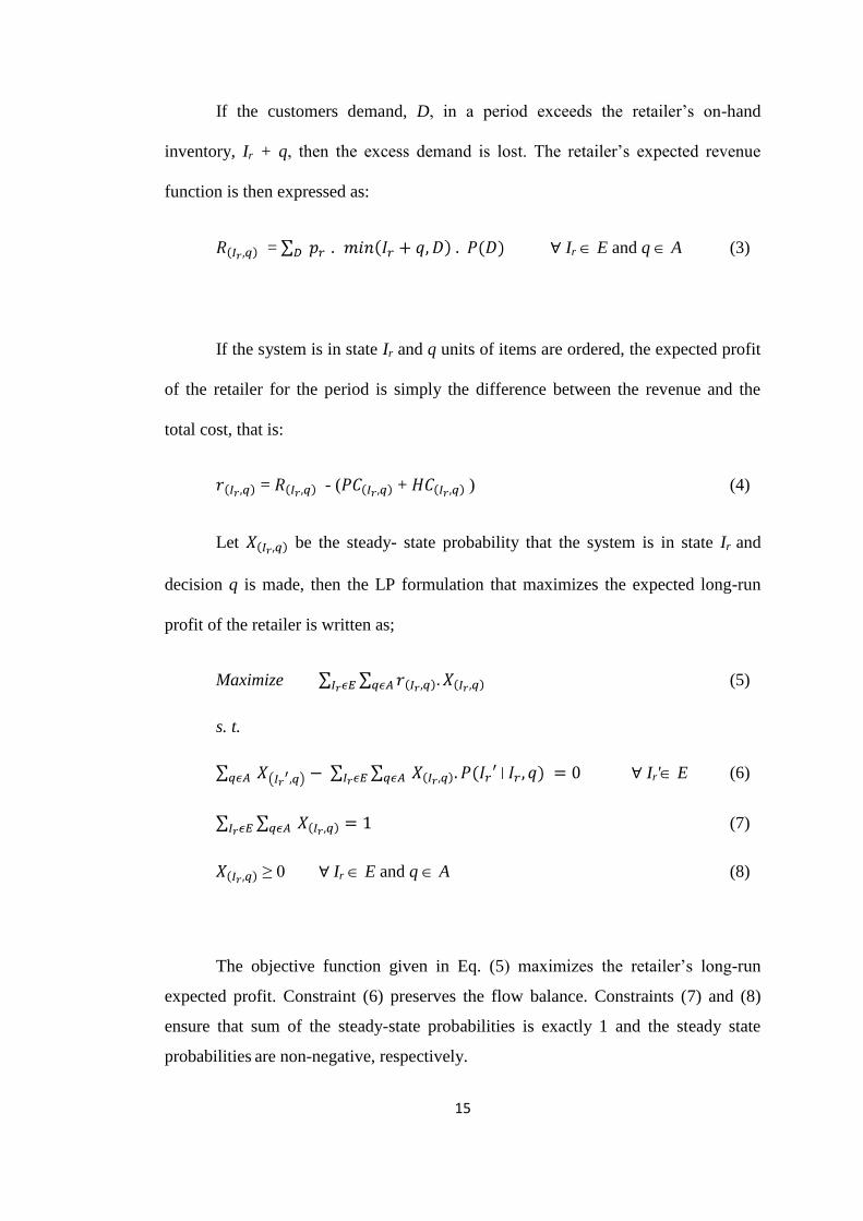
If the customers demand, D, in a period exceeds the retailer‟s on-hand
inventory, Ir + q, then the excess demand is lost. The retailer‟s expected revenue
function is then expressed as:
= Ir E and q A (3)
If the system is in state Ir and q units of items are ordered, the expected profit
of the retailer for the period is simply the difference between the revenue and the
total cost, that is:
= - ( + ) (4)
Let be the steady- state probability that the system is in state Ir and
decision q is made, then the LP formulation that maximizes the expected long-run
profit of the retailer is written as;
Maximize (5)
s. t.
Ir' E (6)
(7)
≥ 0 Ir E and q A (8)
The objective function given in Eq. (5) maximizes the retailer‟s long-run
expected profit. Constraint (6) preserves the flow balance. Constraints (7) and (8)
ensure that sum of the steady-state probabilities is exactly 1 and the steady state
probabilities are non-negative, respectively.
16
In traditional setting, the optimal ordering policy of the retailer is obtained by
the given MDP model. According to the modeled environment in traditional setting,
the retailer uses (s,S) policy in managing his inventory. That is, if the level of
inventory drops below the reorder point s, then the retailer places an order to bring
his inventory level to S.
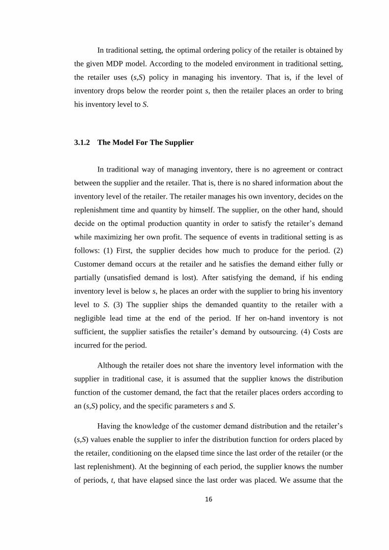
3.1.2 The Model For The Supplier
In traditional way of managing inventory, there is no agreement or contract
between the supplier and the retailer. That is, there is no shared information about the
inventory level of the retailer. The retailer manages his own inventory, decides on the
replenishment time and quantity by himself. The supplier, on the other hand, should
decide on the optimal production quantity in order to satisfy the retailer‟s demand
while maximizing her own profit. The sequence of events in traditional setting is as
follows: (1) First, the supplier decides how much to produce for the period. (2)
Customer demand occurs at the retailer and he satisfies the demand either fully or
partially (unsatisfied demand is lost). After satisfying the demand, if his ending
inventory level is below s, he places an order with the supplier to bring his inventory
level to S. (3) The supplier ships the demanded quantity to the retailer with a
negligible lead time at the end of the period. If her on-hand inventory is not
sufficient, the supplier satisfies the retailer‟s demand by outsourcing. (4) Costs are
incurred for the period.
Although the retailer does not share the inventory level information with the
supplier in traditional case, it is assumed that the supplier knows the distribution
function of the customer demand, the fact that the retailer places orders according to
an (s,S) policy, and the specific parameters s and S.
Having the knowledge of the customer demand distribution and the retailer‟s
(s,S) values enable the supplier to infer the distribution function for orders placed by
the retailer, conditioning on the elapsed time since the last order of the retailer (or the
last replenishment). At the beginning of each period, the supplier knows the number
of periods, t, that have elapsed since the last order was placed. We assume that the
17
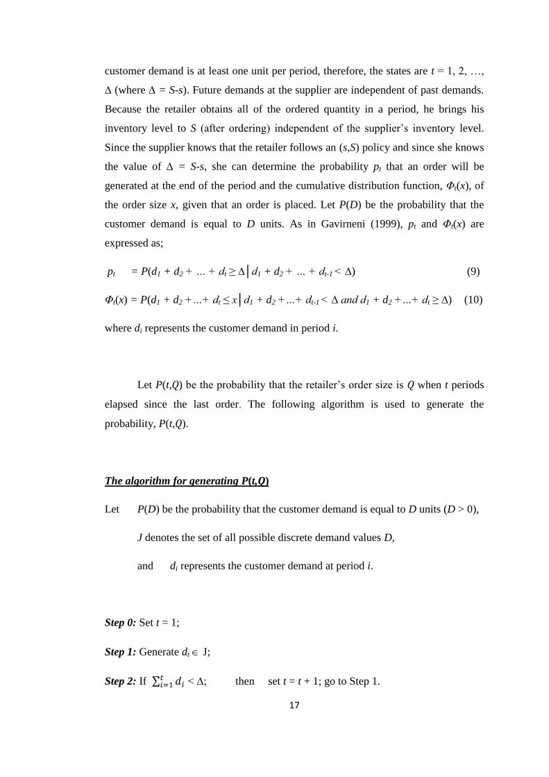
customer demand is at least one unit per period, therefore, the states are t = 1, 2, …,
∆ (where ∆ = S-s). Future demands at the supplier are independent of past demands.
Because the retailer obtains all of the ordered quantity in a period, he brings his
inventory level to S (after ordering) independent of the supplier‟s inventory level.
Since the supplier knows that the retailer follows an (s,S) policy and since she knows
the value of ∆ = S-s, she can determine the probability pt that an order will be
generated at the end of the period and the cumulative distribution function, Φt(x), of
the order size x, given that an order is placed. Let P(D) be the probability that the
customer demand is equal to D units. As in Gavirneni (1999), pt and Φt(x) are
expressed as;
pt = P(d1 + d2 + … + dt ≥ ∆│d1 + d2 + … + dt-1 < ∆) (9)
Φt(x) = P(d1 + d2 +…+ dt ≤ x│d1 + d2 +…+ dt-1 < ∆ and d1 + d2 +…+ dt ≥ ∆) (10)
where di represents the customer demand in period i.
Let P(t,Q) be the probability that the retailer‟s order size is Q when t periods
elapsed since the last order. The following algorithm is used to generate the
probability, P(t,Q).
The algorithm for generating P(t,Q)
Let P(D) be the probability that the customer demand is equal to D units (D > 0),
J denotes the set of all possible discrete demand values D,
and di represents the customer demand at period i.
Step 0: Set t = 1;
Step 1: Generate dt J;
Step 2: If < ∆; then set t = t + 1; go to Step 1.
18
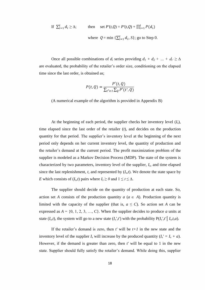
If ≥ ∆; then set P'(t,Q) = P'(t,Q) +
where Q = min { , S}; go to Step 0.
Once all possible combinations of di series providing d1 + d2 + … + dt‟ ≥ ∆
are evaluated, the probability of the retailer‟s order size, conditioning on the elapsed
time since the last order, is obtained as;
(A numerical example of the algorithm is provided in Appendix B)
At the beginning of each period, the supplier checks her inventory level (Is),
time elapsed since the last order of the retailer (t), and decides on the production
quantity for that period. The supplier‟s inventory level at the beginning of the next
period only depends on her current inventory level, the quantity of production and
the retailer‟s demand at the current period. The profit maximization problem of the
supplier is modeled as a Markov Decision Process (MDP). The state of the system is
characterized by two parameters, inventory level of the supplier, Is, and time elapsed
since the last replenishment, t, and represented by (Is,t). We denote the state space by
E which consists of (Is,t) pairs where Is ≥ 0 and 1 ≤ t ≤ ∆.
The supplier should decide on the quantity of production at each state. So,
action set A consists of the production quantity a (a A). Production quantity is
limited with the capacity of the supplier (that is, a ≤ C). So action set A can be
expressed as A = {0, 1, 2, 3, …, C}. When the supplier decides to produce a units at
state (Is,t), the system will go to a new state (Is',t') with the probability P(Is',t'│Is,t,a).
If the retailer‟s demand is zero, then t' will be t+1 in the new state and the
inventory level of the supplier Is will increase by the produced quantity (Is' = Is + a).
However, if the demand is greater than zero, then t' will be equal to 1 in the new
state. Supplier should fully satisfy the retailer‟s demand. While doing this, supplier
19
will use the on-hand inventory (Is+a) first. If it is not enough to satisfy the all
demand, then she will provide the remaining by outsourcing. So, the inventory level
of the supplier at the beginning of the next period, Is', will be zero if the retailer‟s
demand is greater than or equal to the on-hand inventory of the supplier. Otherwise,
Is' will be greater than zero and will be equal to Is + a - Q. As a result, the state
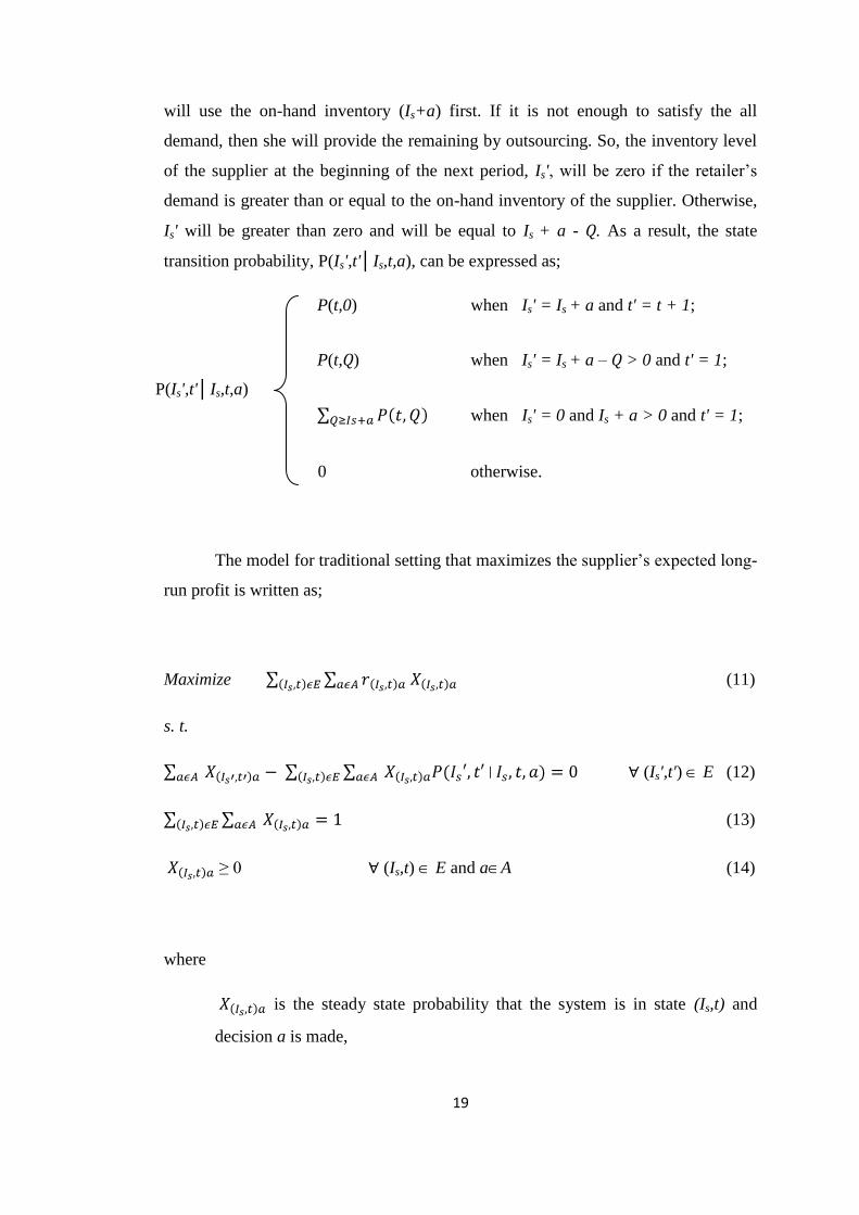
transition probability, P(Is',t'│Is,t,a), can be expressed as;
P(t,0) when Is' = Is + a and t' = t + 1;
P(t,Q) when Is' = Is + a – Q > 0 and t' = 1;
when Is' = 0 and Is + a > 0 and t' = 1;
0 otherwise.
The model for traditional setting that maximizes the supplier‟s expected long-
run profit is written as;
Maximize (11)
s. t.
(Is',t') E (12)
(13)
≥ 0 (Is,t) E and aA (14)
where
is the steady state probability that the system is in state (Is,t) and
decision a is made,
P(Is',t'│Is,t,a)
=
20
and is the expected profit gained if the system is in state (Is,t) and
decision a is made.
The objective function given in (11) maximizes the long run expected average
profit of the supplier. Constraint (12) preserves the flow balance. Constraint (13)
ensures that sum of the steady-state probabilities is exactly 1 and Constraint (14)
ensures that steady state probabilities should be non-negative.
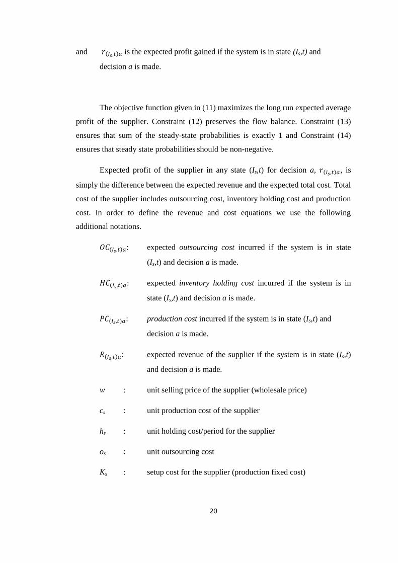
Expected profit of the supplier in any state (Is,t) for decision a, , is
simply the difference between the expected revenue and the expected total cost. Total
cost of the supplier includes outsourcing cost, inventory holding cost and production
cost. In order to define the revenue and cost equations we use the following
additional notations.
: expected outsourcing cost incurred if the system is in state
(Is,t) and decision a is made.
: expected inventory holding cost incurred if the system is in
state (Is,t) and decision a is made.
: production cost incurred if the system is in state (Is,t) and
decision a is made.
: expected revenue of the supplier if the system is in state (Is,t)
and decision a is made.
w : unit selling price of the supplier (wholesale price)
cs : unit production cost of the supplier
hs : unit holding cost/period for the supplier
os : unit outsourcing cost
Ks : setup cost for the supplier (production fixed cost)

21
If the system is in state (Is,t) and decision a is made, then total inventory of
the supplier for that period will be equal to Is + a . If the retailer‟s demand (Q)
exceeds the supplier‟s total inventory, i.e., if Q > Is + a, then the supplier will
outsource Q – (Is + a) units of item. On the other hand, if the demand is less than the
supplier‟s total inventory (Q < Is + a), then the supplier will incur holding cost for (Is
+ a) – Q units of item. So, for a given state (Is,t) and decision a, expected outsourcing
and holding costs are given in Eq. (15) and (16) respectively;
OC(Is,t)a = (15)
HC(Is,t)a = (16)
Production cost of the supplier is defined as a function of the produced
quantity, a. At any state, if the supplier decides to produce a units (a > 0), then she
will charge a fixed setup cost, Ks, and unit production cost cs for each produced unit
of item. That is;
(17)
The revenue of the supplier is independent from the state of the system and
the decision of production quantity, because she should satisfy the retailer‟s demand
fully in any case and she gets w dollars per unit of item dispatched to the retailer.
When the retailer demands Q units of item, then the revenue of the supplier will be
equal to (w . Q). Then the expected revenue of the supplier is as in Eq. (8).
R(Is,t)a = (18)
PC(Is,t)a =
cs . a + Ks for a > 0
0 for a = 0
22
Using the revenue function defined in Eq. (8) and the cost components defined in Eq.
(5), (6) and (7), we obtain the expected profit of the supplier. When the system is in
state (Is,t) and decision a is made, the expected profit, r(Is,t)a , is the difference
between the expected revenue and total cost.
r(Is,t)a = R(Is,t)a - (OC(Is,t)a + HC(Is,t)a + PC(Is,t)a ) (19)
3.2 VMI SETTING
In traditional setting, it is assumed that the end-item demand probabilities and
the retailer‟s inventory policy with its parameter values ((s,S) policy with s and S
values) are the only information known by the supplier. In VMI setting, the inventory
level of the retailer is also available to the supplier and the management of the
retailer‟s inventory is left to the supplier. According to the VMI agreement, the
supplier follows a (z,Z) type policy in managing the retailer‟s inventory. That is, the
retailer sets a minimum inventory level, z, and a maximum inventory level, Z, which
represents the lowest and highest inventory levels, respectively. The supplier decides
not only to the quantity of production but also the quantity of shipment to the retailer.
She should keep the inventory level of the retailer between the specified (z,Z) values.
The sequence of events relating to the replenishment decision under VMI is as
follows: (0) (z,Z) levels are specified by a contract. (1) The supplier examines the
retailer‟s inventory level and decides how much to produce and how much to ship to
the retailer. If the retailer‟s inventory level is below z, then the supplier should make
a replenishment to carry the inventory level between z and Z. (2) The material is
shipped to the retailer with negligible lead time. (3) Demand occurs at the retailer.
(4) Holding costs are incurred.
In traditional case, the fixed order cost of the retailer (can be named as
transportation cost) was charged to the retailer. In VMI setting, however, this cost
will be shared between the participants in different ratios.
23
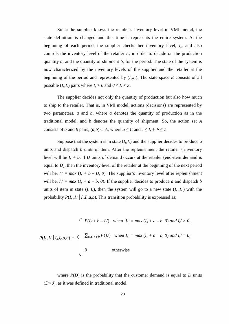
Since the supplier knows the retailer‟s inventory level in VMI model, the
state definition is changed and this time it represents the entire system. At the
beginning of each period, the supplier checks her inventory level, Is, and also
controls the inventory level of the retailer Ir, in order to decide on the production
quantity a, and the quantity of shipment b, for the period. The state of the system is
now characterized by the inventory levels of the supplier and the retailer at the
beginning of the period and represented by (Is,Ir). The state space E consists of all
possible (Is,Ir) pairs where Is ≥ 0 and 0 ≤ Ir ≤ Z.
The supplier decides not only the quantity of production but also how much
to ship to the retailer. That is, in VMI model, actions (decisions) are represented by
two parameters, a and b, where a denotes the quantity of production as in the
traditional model, and b denotes the quantity of shipment. So, the action set A
consists of a and b pairs, (a,b) A, where a ≤ C and z ≤ Ir + b ≤ Z.
Suppose that the system is in state (Is,Ir) and the supplier decides to produce a
units and dispatch b units of item. After the replenishment the retailer‟s inventory
level will be Ir + b. If D units of demand occurs at the retailer (end-item demand is
equal to D), then the inventory level of the retailer at the beginning of the next period
will be, Ir' = max (Ir + b – D, 0). The supplier‟s inventory level after replenishment
will be, Is' = max (Is + a – b, 0). If the supplier decides to produce a and dispatch b
units of item in state (Is,Ir), then the system will go to a new state (Is',Ir') with the
probability P(Is',Ir'│Is,Ir,a,b). This transition probability is expressed as;
P(Ir + b – Ir') when Is' = max (Is + a – b, 0) and Ir' > 0;
when Is' = max (Is + a – b, 0) and Ir' = 0;
0 otherwise
where P(D) is the probability that the customer demand is equal to D units
(D>0), as it was defined in traditional model.
P(Is',Ir'│Is,Ir,a,b) =
24
Let be the steady-state probability that the system is in state (Is,Ir)
and decision (a,b) is made. Then, the LP formulation for VMI setting that maximizes
the supplier‟s expected long-run profit is written as;
Maximize (20)
s. t.
(Is',Ir') E (21)
(22)
≥ 0 (Is,Ir) E and (a,b) A (23)
where denotes the expected profit gained if system is in state (Is,Ir) and
decision (a,b) is made.
The objective function given in Eq. (20) maximizes the long run expected
average profit of the supplier for a given (z,Z) band. Constraint (21) preserves the
flow balance. Constraints (22) and (23) ensure that sum of the steady-state
probabilities is exactly 1 and the steady state probabilities are non-negative,
respectively.
In order to generate the equation for the profit of the supplier when the
system is in state (Is,Ir) and decision (a,b) is made , we should first
specify the revenue and cost equations. In VMI case, there is an additional cost
component for the supplier when compared with the traditional model, which is
dispatching cost (or transportation cost).
25
Additional notation for VMI setting is provided below:
: dispatching cost (transportation cost) incurred if the system is
in state (Is,Ir) and decision (a,b) is made.
: expected outsourcing cost incurred if the system is in state
(Is,Ir) and decision (a,b) is made.
: expected inventory holding cost incurred if the system is in
state (Is,Ir) and decision (a,b) is made.
: production cost incurred if the system is in state (Is,Ir) and
decision (a,b) is made.
: expected revenue of the supplier if the system is in state (Is,Ir)
and decision (a,b) is made.
When the supplier decides to produce a units of item in state (Is,Ir), then her
inventory level will be Is + a just before the shipment. If the supplier dispatches b
units of item to the retailer, then she will incur holding cost for Is + a – b units of
item if b < Is + a. However, if the dispatching quantity b is greater than Is + a, then
outsourcing cost will be incurred for b – (Is + a) units of item. So, holding and
outsourcing cost equations will be as follows:
= os . max (b – Is - a, 0) (24)
= hs . max (Is + a - b, 0) (25)
Each time the supplier makes a replenishment, a specified fraction (denoted
as αs) of the retailer‟s fixed order cost will be charged to the supplier as dispatching
cost.
26
αs . Kr for b > 0
0 for b = 0
Production cost expression in VMI model is the same with the expression in
traditional setting. At any state, if the supplier decides to produce a units (a > 0),
then she will charge a fixed setup cost, Ks, and unit production cost cs for each
produced unit of item. That is;
(27)
If the supplier dispatches b units of item in any state, then the revenue of the
supplier is simply the multiplication of wholesale price, w, by dispatch quantity b.
That is,
= w . b (28)
Profit function of the supplier can now be expressed by using the revenue
function in Eq. (28) and cost components described in Eqns. (24), (25), (26) and (27).
r(Is,Ir)(a,b) = - ( + +
+ ) (29)
In VMI setting, the expected profit of the retailer is also calculated within the
model. The notation that is related with the cost, revenue and profit of the retailer in
PC(Is,Ir)(a,b) =
cs . a + Ks for a > 0
0 for a = 0
(26) =
27
VMI setting is given below. In order to specify „the retailer‟, superscript „R‟ is used
in representation.
: purchasing cost (includes fixed and variable cost ) of the
retailer when the system is in state (Is,Ir) and decision (a,b) is
made.
: expected inventory holding cost of the retailer if the system is
in state (Is,Ir) and decision (a,b) is made.
: expected revenue of the retailer if the system is in state (Is,Ir)
and decision (a,b) is made.
: expected profit of the retailer if system is in state (Is,Ir) and
decision (a,b) is made.
pr : unit selling price of the retailer (end-item price)
hr : unit holding cost/period for the retailer
When the system is in state (Is,Ir) and the supplier decides to dispatch b units
of item to the supplier, the retailer‟s inventory level will be Ir + b before the
customer demand occurs. If the retailer‟s inventory level after replenishment (Ir + b)
is enough to fully satisfy the demand, i.e., if Ir + b ≥ D, then the retailer‟s revenue
will be (pr D) and he will incur holding cost for the remaining Ir + b – D units of
inventory, after satisfying the demand. On the other hand, if the demand is greater
than on-hand inventory, excess demand will be lost as in the traditional case. The
holding cost and the revenue functions are provided in Eqns. (30) and (31),
respectively.
= (Is,Ir) E , (a,b) A (30)
28
= (Is,Ir) E, (a,b) A (31)
One other cost component for the retailer is purchasing cost, which contains
ordering fixed cost and variable cost. Each time the supplier makes a replenishment,
the retailer will pay w for each unit. Ordering fixed cost (transportation cost) is
shared between the supplier and the retailer in the VMI setting. So, the retailer will
pay the specified fraction (will be denoted as αr ) of fixed cost. (αr = 1 - αs).
Purchasing cost function of the retailer is given in Eq. (32).
Expected profit of the retailer in state (Is,Ir) when decision (a,b) is made, can
now be expressed as;
= – ( + ) (33)
We defined as the steady-state probability that the system is in
state (Is,Ir) and decision (a,b) is made. So, the expected total long-run profit of the
retailer in VMI setting is obtained by the following summation:
. (34)
=
(1-αs) . Kr + w . b for b > 0
0 for b = 0
(32)
29
3.3 CENTRALIZED SETTING
In the centralized setting, the supplier and the retailer act as a single firm for a
unique objective. The decisions, concerning production and replenishment, are
assumed to be made with the focus of maximizing the total supply chain profit. The
supplier, which has full information about the retailer and the chain, can be
considered as the central decision maker. She aims to maximize the total chain profit
by managing the inventory in the supply chain.
The sequence of events in a period relating to the replenishment decision is
the same with the VMI setting and as follows: (1) The supplier, as a central decision
maker, reviews her own and the retailer‟s inventory level, and then decides on the
production and dispatch quantity. (2) The material is shipped to the retailer with
negligible lead time. (3) Demand occurs at the retailer. (4) Costs are incurred.
The state of the system represents the entire supply chain in the centralized
setting and defined as the inventory levels of the supplier and the retailer at the
beginning of each period, (Is,Ir). The definition of the state is the same with the VMI
setting. However, in centralized case, the retailer‟s inventory level is not bounded by
an agreement. So, the state space E consists of all (Is,Ir) pairs where Is ≥ 0 and Ir ≥ 0.
The decisions of production and replenishment quantities are made by the
supplier after checking the inventory levels at the beginning of each period. The
action set A is composed of the production and dispatch quantities, a and b
respectively, where 0 ≤ a ≤ C and b ≥ 0. After the action is taken, customer demand
occurs at the retailer and the system goes to a new state, (Is',Ir'), with the probability
P(Is',Ir'│Is,Ir,a,b), which is expressed in VMI setting.
The LP formulation for centralized setting that maximizes the expected long-
run profit of the supply chain is written as;
30
Maximize (35)
s. t.
(Is',Ir') E (36)
(37)
≥ 0 (Is,Ir) E and (a,b) A (38)
where
is the steady-state probability that the system is in state (Is,Ir) and
decision (a,b) is made;
and denotes the expected profit of the supply chain if the system is in
state (Is,Ir) and decision (a,b) is made.
All cost components of the retailer and the supplier in the centralized setting
are the same with those defined and expressed in the VMI setting. The expected
profit of the supply chain in state (Is,Ir) when decision (a,b) is made, ,
is the sum of the profit of each member. That is;
(39)
where and are the expected profits of the supplier and
the retailer, respectively, and expressed in Eqns. (19) and (23).
31
CHAPTER 4
COMPUTATIONAL STUDY
In this section, a computational study is performed in order to investigate the
benefits of VMI and to examine the performance of the agreement in coordinating
the supply chain. The benefit of VMI on the profits of the retailer, the supplier and
the total supply chain are evaluated separately and the effects of the system
parameters to the benefit of VMI on profits are investigated. In addition to the
benefits of the VMI over the traditional setting, the performance of VMI in
coordinating the supply chain is examined.
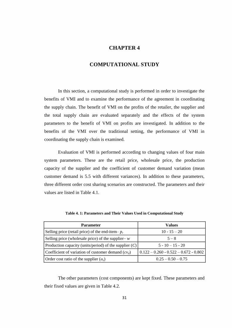
Evaluation of VMI is performed according to changing values of four main
system parameters. These are the retail price, wholesale price, the production
capacity of the supplier and the coefficient of customer demand variation (mean
customer demand is 5.5 with different variances). In addition to these parameters,
three different order cost sharing scenarios are constructed. The parameters and their
values are listed in Table 4.1.
Table 4. 1: Parameters and Their Values Used in Computational Study
Parameter Values
Selling price (retail price) of the end-item– pr 10 - 15 – 20
Selling price (wholesale price) of the supplier– w 5 – 8
Production capacity (units/period) of the supplier (C) 5 - 10 – 15 - 20
Coefficient of variation of customer demand (cvd) 0.122 – 0.260 - 0.522 – 0.672 - 0.802
Order cost ratio of the supplier (αs) 0.25 – 0.50 – 0.75
The other parameters (cost components) are kept fixed. These parameters and
their fixed values are given in Table 4.2.
32
Table 4. 2: Cost Parameters and Fixed Values Used in Computational Study
Cost Component Cost
Holding cost of the retailer (hr) 1.2
Holding cost of the supplier (hs) 0.5
Order cost of the retailer (Kr) 10
Production setup cost of the supplier (Ks) 20
Unit production cost (p) 1
Unit outsource cost (os) 11
4.1 Benefit of VMI on Supplier’s Profit:
In analyzing the benefits of VMI on supplier‟s profit, we assume that the
supplier is the powerful player in the chain, and the values of contract parameters, z
and Z, are set by her. However, in order to encourage the retailer to participate in
such a VMI agreement, she has to provide that the retailer must be better than the
traditional setting in terms of profit with the decided values of (z,Z) levels. Among
all possible levels that satisfy the retailer‟s criteria, the supplier selects the one that
maximizes her profit.
In the computational study, for each parameter set, the profits of the retailer
and the supplier are calculated under all (z,Z) levels (0 ≤ z ≤ Z) with a complete
enumeration, and the (z,Z) level satisfying the mentioned criteria is obtained.
For each set of parameter, the profit of the supplier under VMI is compared to
the profit in traditional setting, and the benefit of VMI over traditional setting is
analyzed under different values of system parameters. For each parameter set, the
profit value of the supplier under the traditional and the VMI setting is provided in
Appendix C.
33
4.1.1 Effect of Demand Variation:
In the VMI setting, the replenishment decision is made by the supplier and
this provides her flexibility in terms of the dispatch quantity. She can replenish the
retailer with any quantity as soon as she guarantees the inventory level of the retailer
after replenishment is kept between the specified (z,Z) levels. The specified values of
these levels, z and Z, determine the flexibility of the supplier in VMI setting. As the
difference between these levels (Z - z) increase, the flexibility increases.
In contrast to the traditional setting, the supplier does not face a demand by
the retailer in VMI setting that should be fully satisfied. Because of the gained
flexibility in dispatch quantity, the supplier does not use the expensive outsource
option in VMI. In addition, since the supplier has full information about the retailer
and flexible in replenishment quantity, she operates on just-in-time basis; that is, as
soon as she make a production, she dispatches all produced items to the retailer and
does not carry inventory. If the specified (z,Z) levels in the VMI agreement provide
enough flexibility to the supplier to keep the retailer‟s inventory levels between the
specified values without outsourcing and holding inventory; in the long-run, the
expected revenue and the profit of the supplier are not affected by the coefficient of
customer demand variation as long as the mean demand is the same.
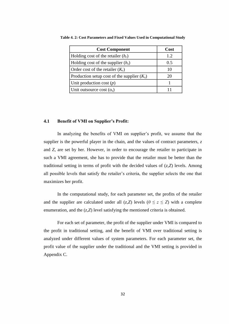
Figure 4.1 monitors the effect of customer demand variation to the supplier‟s
profit in traditional and VMI setting (C=15; pr = 15; αs = 0.25 for this example). It
is seen that, the expected profit of the supplier in VMI setting does not change with
the coefficient of variation. The (z,Z) levels, set by the supplier at each cvd value in
this example, are the optimal levels for her and these levels are also acceptable by the
retailer in VMI setting. For increasing values of cvd in this example, the (z,Z) levels,
set by the supplier, are (7,21), (8,22), (10,24), (10,24) and (10,24), respectively. At
each pair, the difference between the maximum and the minimum level (Z-z) is 14.
So, when the retailer‟s inventory level drops below z, the supplier makes a
production with full capacity (a = 15) and dispatches all produced items to the
retailer. With this policy, the supplier does not incur any holding and outsourcing
cost. In addition, she minimizes the unit production cost by allocating the fixed cost
to the full capacity and reaches the optimal profit. Under such a situation, the
34
expected profit of the supplier is not affected by different values of coefficient of
variation, since the mean demand is the same at each value.
Figure 4. 1: Profit of The Supplier vs Coefficient of Variation (cvd) Under Traditional and VMI
Setting (C = 15; pr = 15; αs = 0.25)
In traditional case, however, the supplier periodically faces demand from the
retailer, and she infers the distribution of this demand by using customer demand
distribution and the (s,S) values as expressed in Eqns. (9) and (10). Changing values
of coefficient of customer demand variation and (s,S) parameters yields different
demand distributions, inferred by the supplier. Therefore, the expected profit of the
supplier in traditional setting is affected by the coefficient of customer demand
variation.
In Figure 4.1, when the wholesale price is low (w = 5), the expected profit of
the supplier decreases with increasing values of the coefficient of customer demand
variation in traditional setting. As the demand variation increases, the difference
between the order-up-to level (S) and the reorder point (s) is decreased by the retailer
to become more sensitive to the variations on demand, and the retailer keeps more
safety stock. Decreased (S-s) provides the supplier to better infer the distribution of
the retailer orders. However, as the difference (S-s) decreases, the retailer‟s order
0
5
10
15
20
25
30
35
0.000 0.100 0.200 0.300 0.400 0.500 0.600 0.700 0.800 0.900
Pro
fit
/ P
eri
od
cvd
Profit of Supplier versus cvd
w=8 (VMI) w=8 (Trad) w=5 (VMI) w=5 (Trad)
35
frequency increases in traditional setting. That is, he is replenished by the supplier
more frequently with smaller quantities. Due to the decreased dispatch quantity, the
supplier incurs higher inventory holding cost. Although the revenue of the supplier is
also increased with the increasing values of the reorder point (s) at high variance
case, increasing holding cost is the most important factor in decreasing profits. For
the higher value of wholesale price (w=8), the profit is maximum when the
coefficient of demand variation is low. With increasing values of cvd, the profit
initially decreases and reaches minimum at moderate values of cvd, then increases
slightly. For w=8, at higher values of cvd, the increase in the revenue is slightly
greater than the increase in holding cost, which results in increasing profit.
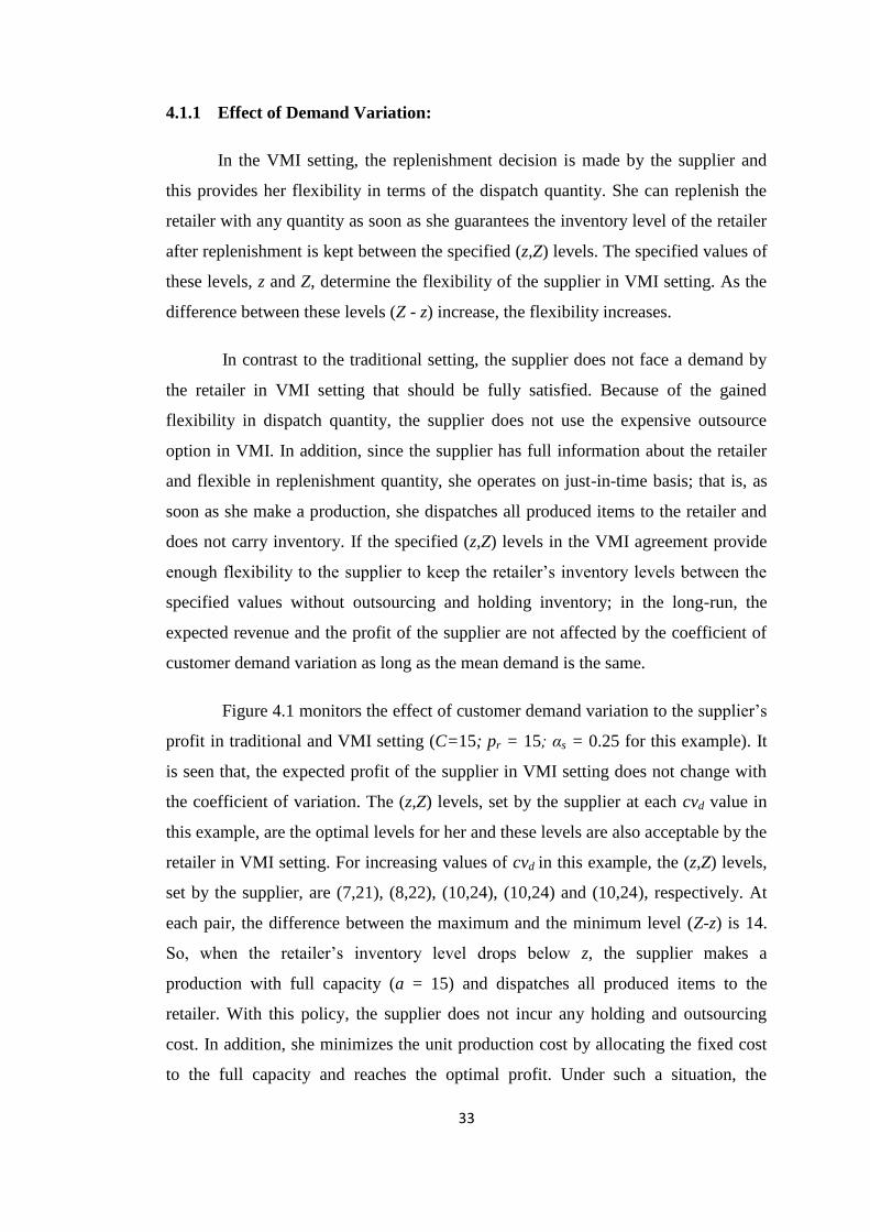
The effect of customer demand variation to the benefit of VMI is displayed in
Figure 4.2. The benefit of VMI increases with increasing demand variation when the
wholesale price is low. For a higher wholesale price, VMI is most beneficial at
moderate values of variation and provide 25% increase on profit.
Figure 4. 2: Benefit of VMI on Supplier’s Profit vs Coefficient of Variation
(C = 15; pr = 15; αs = 0.25)
4.1.2 Effect of Capacity
Figure 4.3 displays the effect of the capacity to the benefit of VMI on the
supplier‟s profit. For every value of capacity and each coefficient of variation of
10
15
20
25
30
35
40
45
50
55
60
0.000 0.100 0.200 0.300 0.400 0.500 0.600 0.700 0.800 0.900
% B
en
efi
t
cvd
Benefit of VMI on Supplier's Profit versus cvd
w=5
w=8
36
customer demand, since they show similar patterns, the percentage benefits are
averaged over all the retail and wholesale prices in the figure.
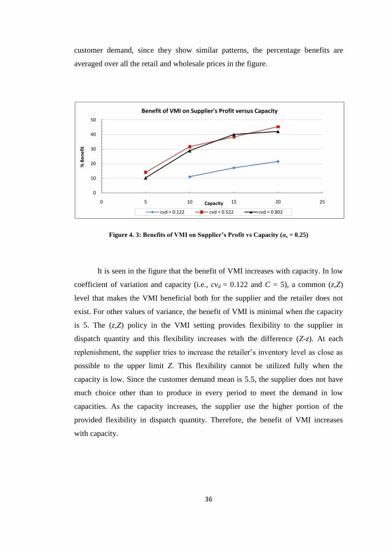
Figure 4. 3: Benefits of VMI on Supplier’s Profit vs Capacity (αs = 0.25)
It is seen in the figure that the benefit of VMI increases with capacity. In low
coefficient of variation and capacity (i.e., cvd = 0.122 and C = 5), a common (z,Z)
level that makes the VMI beneficial both for the supplier and the retailer does not
exist. For other values of variance, the benefit of VMI is minimal when the capacity
is 5. The (z,Z) policy in the VMI setting provides flexibility to the supplier in
dispatch quantity and this flexibility increases with the difference (Z-z). At each
replenishment, the supplier tries to increase the retailer‟s inventory level as close as
possible to the upper limit Z. This flexibility cannot be utilized fully when the
capacity is low. Since the customer demand mean is 5.5, the supplier does not have
much choice other than to produce in every period to meet the demand in low
capacities. As the capacity increases, the supplier use the higher portion of the
provided flexibility in dispatch quantity. Therefore, the benefit of VMI increases
with capacity.
0
10
20
30
40
50
0 5 10 15 20 25
% B
en
efi
t
Capacity
Benefit of VMI on Supplier's Profit versus Capacity
cvd = 0.122 cvd = 0.522 cvd = 0.802
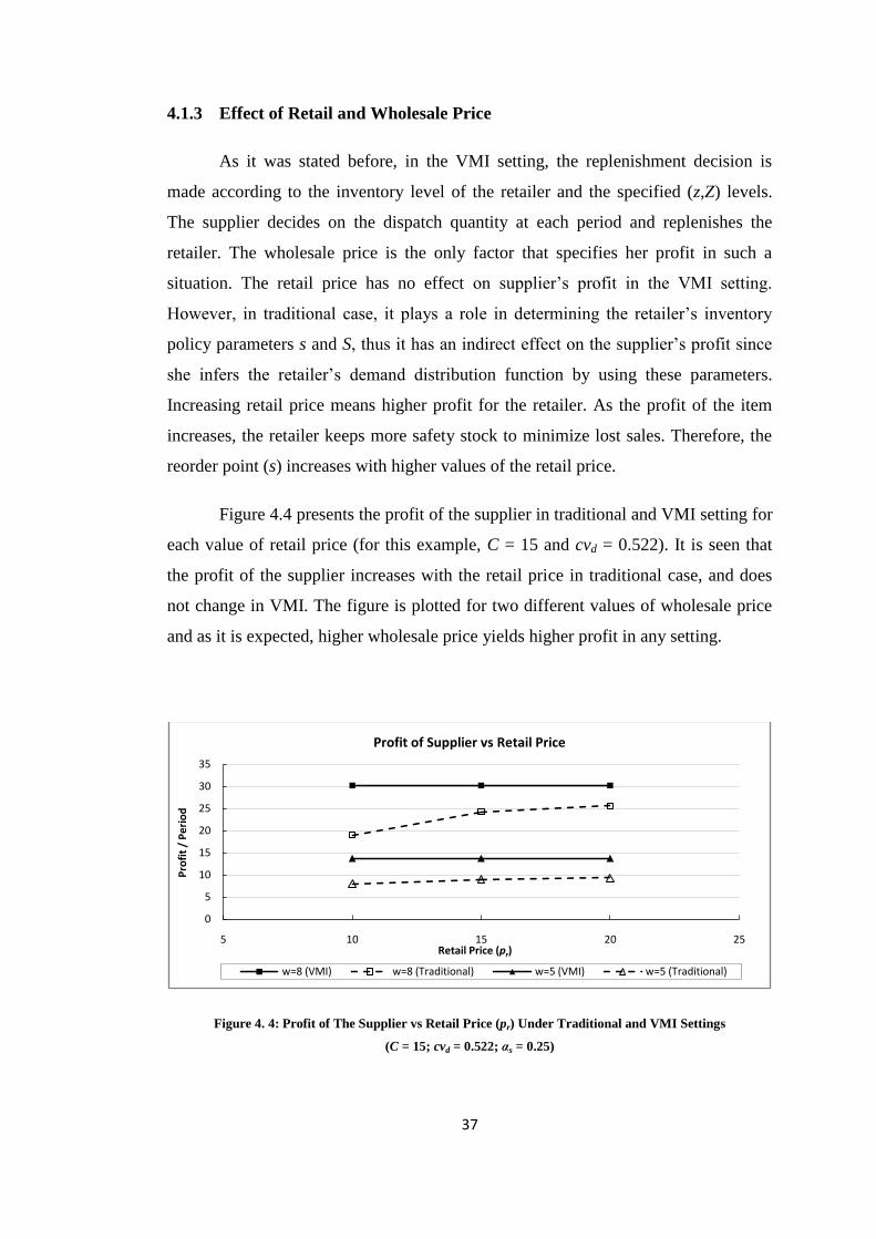
37
4.1.3 Effect of Retail and Wholesale Price
As it was stated before, in the VMI setting, the replenishment decision is
made according to the inventory level of the retailer and the specified (z,Z) levels.
The supplier decides on the dispatch quantity at each period and replenishes the
retailer. The wholesale price is the only factor that specifies her profit in such a
situation. The retail price has no effect on supplier‟s profit in the VMI setting.
However, in traditional case, it plays a role in determining the retailer‟s inventory
policy parameters s and S, thus it has an indirect effect on the supplier‟s profit since
she infers the retailer‟s demand distribution function by using these parameters.
Increasing retail price means higher profit for the retailer. As the profit of the item
increases, the retailer keeps more safety stock to minimize lost sales. Therefore, the
reorder point (s) increases with higher values of the retail price.
Figure 4.4 presents the profit of the supplier in traditional and VMI setting for
each value of retail price (for this example, C = 15 and cvd = 0.522). It is seen that
the profit of the supplier increases with the retail price in traditional case, and does
not change in VMI. The figure is plotted for two different values of wholesale price
and as it is expected, higher wholesale price yields higher profit in any setting.
Figure 4. 4: Profit of The Supplier vs Retail Price (pr) Under Traditional and VMI Settings
(C = 15; cvd = 0.522; αs = 0.25)
0
5
10
15
20
25
30
35
5 10 15 20 25
Pro
fit
/ P
eri
od
Retail Price (pr)
Profit of Supplier vs Retail Price
w=8 (VMI) w=8 (Traditional) w=5 (VMI) w=5 (Traditional)
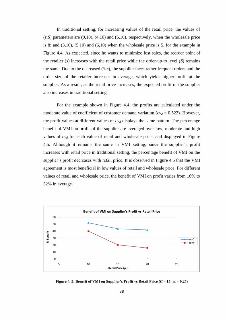
38
In traditional setting, for increasing values of the retail price, the values of
(s,S) parameters are (0,10), (4,10) and (6,10), respectively, when the wholesale price
is 8; and (3,10), (5,10) and (6,10) when the wholesale price is 5, for the example in
Figure 4.4. As expected, since he wants to minimize lost sales, the reorder point of
the retailer (s) increases with the retail price while the order-up-to level (S) remains
the same. Due to the decreased (S-s), the supplier faces rather frequent orders and the
order size of the retailer increases in average, which yields higher profit at the
supplier. As a result, as the retail price increases, the expected profit of the supplier
also increases in traditional setting.
For the example shown in Figure 4.4, the profits are calculated under the
moderate value of coefficient of customer demand variation (cvd = 0.522). However,
the profit values at different values of cvd displays the same pattern. The percentage
benefit of VMI on profit of the supplier are averaged over low, moderate and high
values of cvd for each value of retail and wholesale price, and displayed in Figure
4.5. Although it remains the same in VMI setting; since the supplier‟s profit
increases with retail price in traditional setting, the percentage benefit of VMI on the
supplier‟s profit decreases with retail price. It is observed in Figure 4.5 that the VMI
agreement is most beneficial in low values of retail and wholesale price. For different
values of retail and wholesale price, the benefit of VMI on profit varies from 16% to
52% in average.
Figure 4. 5: Benefit of VMI on Supplier’s Profit vs Retail Price (C = 15; αs = 0.25)
0
10
20
30
40
50
60
5 10 15 20 25
% B
en
efi
t
Retail Price (pr)
Benefit of VMI on Supplier's Profit vs Retail Price
w=5w=8
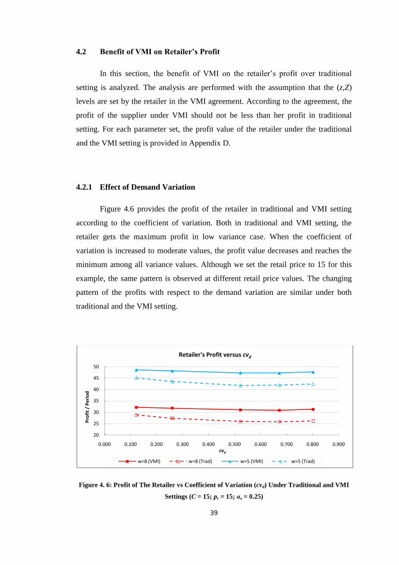
39
4.2 Benefit of VMI on Retailer’s Profit
In this section, the benefit of VMI on the retailer‟s profit over traditional
setting is analyzed. The analysis are performed with the assumption that the (z,Z)
levels are set by the retailer in the VMI agreement. According to the agreement, the
profit of the supplier under VMI should not be less than her profit in traditional
setting. For each parameter set, the profit value of the retailer under the traditional
and the VMI setting is provided in Appendix D.
4.2.1 Effect of Demand Variation
Figure 4.6 provides the profit of the retailer in traditional and VMI setting
according to the coefficient of variation. Both in traditional and VMI setting, the
retailer gets the maximum profit in low variance case. When the coefficient of
variation is increased to moderate values, the profit value decreases and reaches the
minimum among all variance values. Although we set the retail price to 15 for this
example, the same pattern is observed at different retail price values. The changing
pattern of the profits with respect to the demand variation are similar under both
traditional and the VMI setting.
Figure 4. 6: Profit of The Retailer vs Coefficient of Variation (cvd) Under Traditional and VMI
Settings (C = 15; pr = 15; αs = 0.25)
20
25
30
35
40
45
50
0.000 0.100 0.200 0.300 0.400 0.500 0.600 0.700 0.800 0.900
Pro
fit
/ P
eri
od
cvd
Retailer's Profit versus cvd
w=8 (VMI) w=8 (Trad) w=5 (VMI) w=5 (Trad)
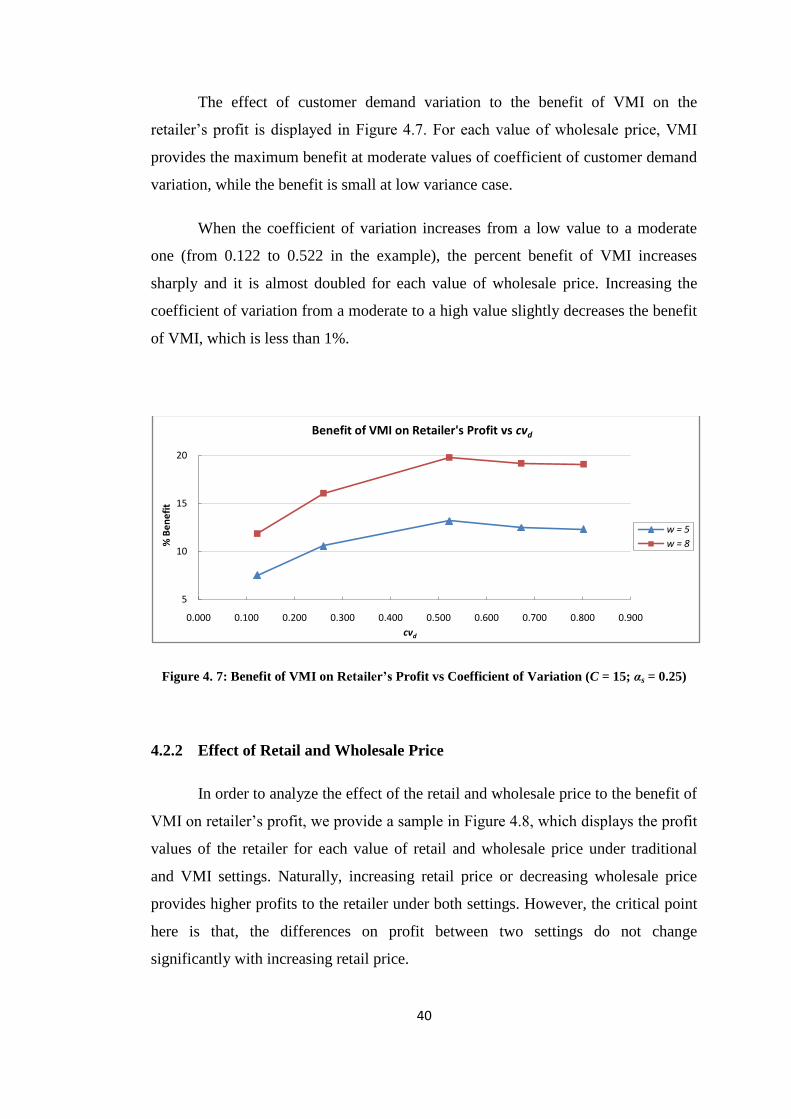
40
The effect of customer demand variation to the benefit of VMI on the
retailer‟s profit is displayed in Figure 4.7. For each value of wholesale price, VMI
provides the maximum benefit at moderate values of coefficient of customer demand
variation, while the benefit is small at low variance case.
When the coefficient of variation increases from a low value to a moderate
one (from 0.122 to 0.522 in the example), the percent benefit of VMI increases
sharply and it is almost doubled for each value of wholesale price. Increasing the
coefficient of variation from a moderate to a high value slightly decreases the benefit
of VMI, which is less than 1%.
Figure 4. 7: Benefit of VMI on Retailer’s Profit vs Coefficient of Variation (C = 15; αs = 0.25)
4.2.2 Effect of Retail and Wholesale Price
In order to analyze the effect of the retail and wholesale price to the benefit of
VMI on retailer‟s profit, we provide a sample in Figure 4.8, which displays the profit
values of the retailer for each value of retail and wholesale price under traditional
and VMI settings. Naturally, increasing retail price or decreasing wholesale price
provides higher profits to the retailer under both settings. However, the critical point
here is that, the differences on profit between two settings do not change
significantly with increasing retail price.
5
10
15
20
0.000 0.100 0.200 0.300 0.400 0.500 0.600 0.700 0.800 0.900
% B
en
efi
t
cvd
Benefit of VMI on Retailer's Profit vs cvd
w = 5
w = 8
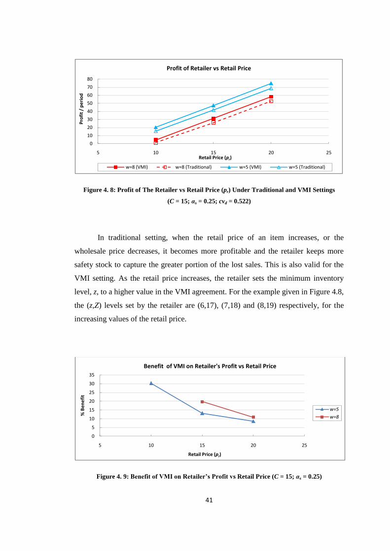
41
Figure 4. 8: Profit of The Retailer vs Retail Price (pr) Under Traditional and VMI Settings
(C = 15; αs = 0.25; cvd = 0.522)
In traditional setting, when the retail price of an item increases, or the
wholesale price decreases, it becomes more profitable and the retailer keeps more
safety stock to capture the greater portion of the lost sales. This is also valid for the
VMI setting. As the retail price increases, the retailer sets the minimum inventory
level, z, to a higher value in the VMI agreement. For the example given in Figure 4.8,
the (z,Z) levels set by the retailer are (6,17), (7,18) and (8,19) respectively, for the
increasing values of the retail price.
Figure 4. 9: Benefit of VMI on Retailer’s Profit vs Retail Price (C = 15; αs = 0.25)
0
10
20
30
40
50
60
70
80
5 10 15 20 25
Pro
fit
/ p
eri
od
Retail Price (pr)
Profit of Retailer vs Retail Price
w=8 (VMI) w=8 (Traditional) w=5 (VMI) w=5 (Traditional)
0
5
10
15
20
25
30
35
5 10 15 20 25
% B
en
efi
t
Retail Price (pr)
Benefit of VMI on Retailer's Profit vs Retail Price
w=5
w=8
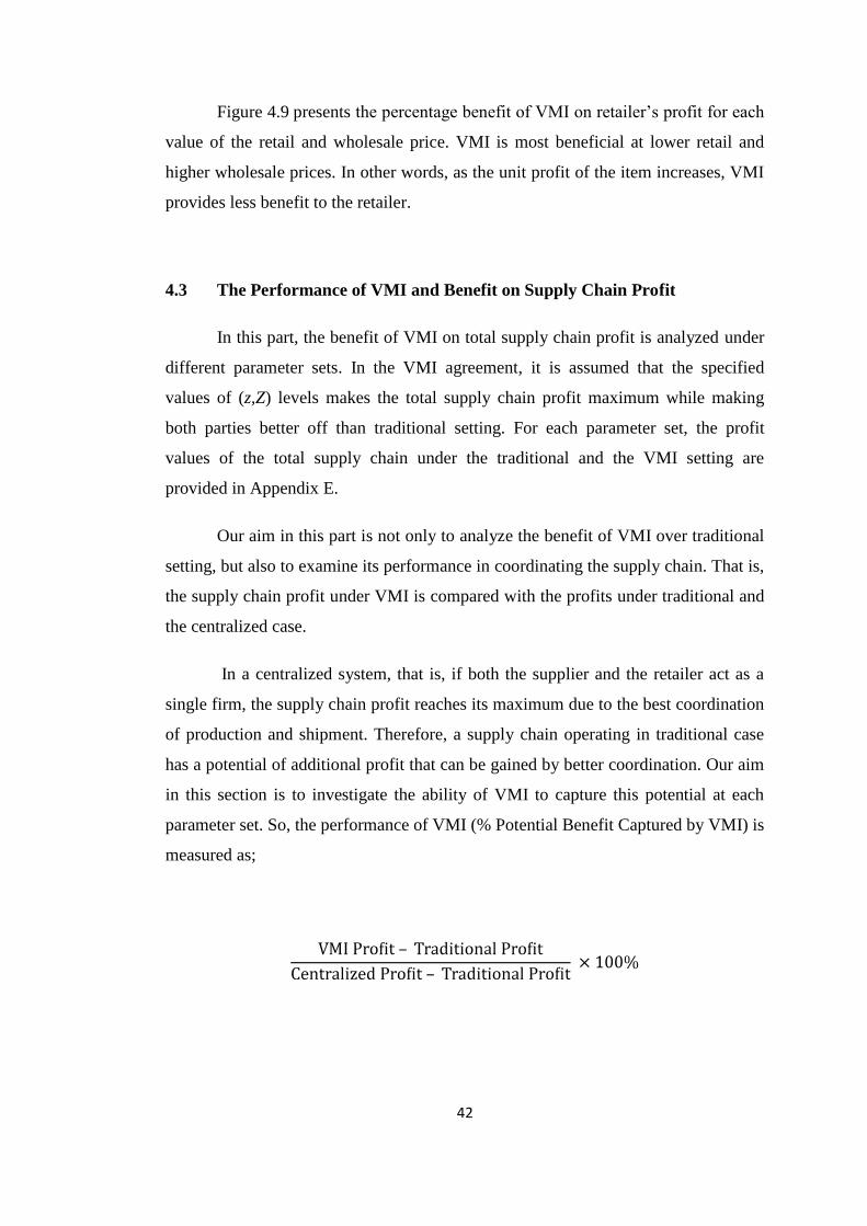
42
Figure 4.9 presents the percentage benefit of VMI on retailer‟s profit for each
value of the retail and wholesale price. VMI is most beneficial at lower retail and
higher wholesale prices. In other words, as the unit profit of the item increases, VMI
provides less benefit to the retailer.
4.3 The Performance of VMI and Benefit on Supply Chain Profit
In this part, the benefit of VMI on total supply chain profit is analyzed under
different parameter sets. In the VMI agreement, it is assumed that the specified
values of (z,Z) levels makes the total supply chain profit maximum while making
both parties better off than traditional setting. For each parameter set, the profit
values of the total supply chain under the traditional and the VMI setting are
provided in Appendix E.
Our aim in this part is not only to analyze the benefit of VMI over traditional
setting, but also to examine its performance in coordinating the supply chain. That is,
the supply chain profit under VMI is compared with the profits under traditional and
the centralized case.
In a centralized system, that is, if both the supplier and the retailer act as a
single firm, the supply chain profit reaches its maximum due to the best coordination
of production and shipment. Therefore, a supply chain operating in traditional case
has a potential of additional profit that can be gained by better coordination. Our aim
in this section is to investigate the ability of VMI to capture this potential at each
parameter set. So, the performance of VMI (% Potential Benefit Captured by VMI) is
measured as;
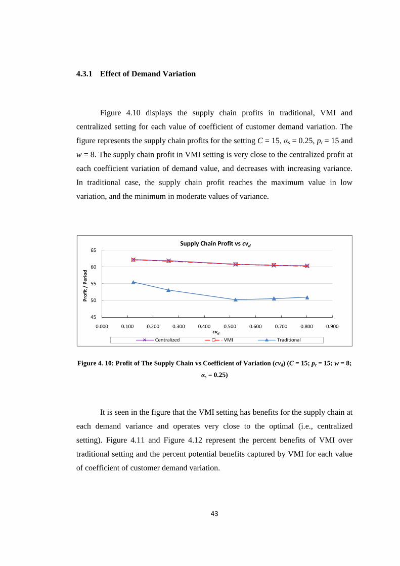
43
4.3.1 Effect of Demand Variation
Figure 4.10 displays the supply chain profits in traditional, VMI and
centralized setting for each value of coefficient of customer demand variation. The
figure represents the supply chain profits for the setting C = 15, αs = 0.25, pr = 15 and
w = 8. The supply chain profit in VMI setting is very close to the centralized profit at
each coefficient variation of demand value, and decreases with increasing variance.
In traditional case, the supply chain profit reaches the maximum value in low
variation, and the minimum in moderate values of variance.
Figure 4. 10: Profit of The Supply Chain vs Coefficient of Variation (cvd) (C = 15; pr = 15; w = 8;
αs = 0.25)
It is seen in the figure that the VMI setting has benefits for the supply chain at
each demand variance and operates very close to the optimal (i.e., centralized
setting). Figure 4.11 and Figure 4.12 represent the percent benefits of VMI over
traditional setting and the percent potential benefits captured by VMI for each value
of coefficient of customer demand variation.
45
50
55
60
65
0.000 0.100 0.200 0.300 0.400 0.500 0.600 0.700 0.800 0.900
Pro
fit
/ P
eri
od
cvd
Supply Chain Profit vs cvd
Centralized VMI Traditional
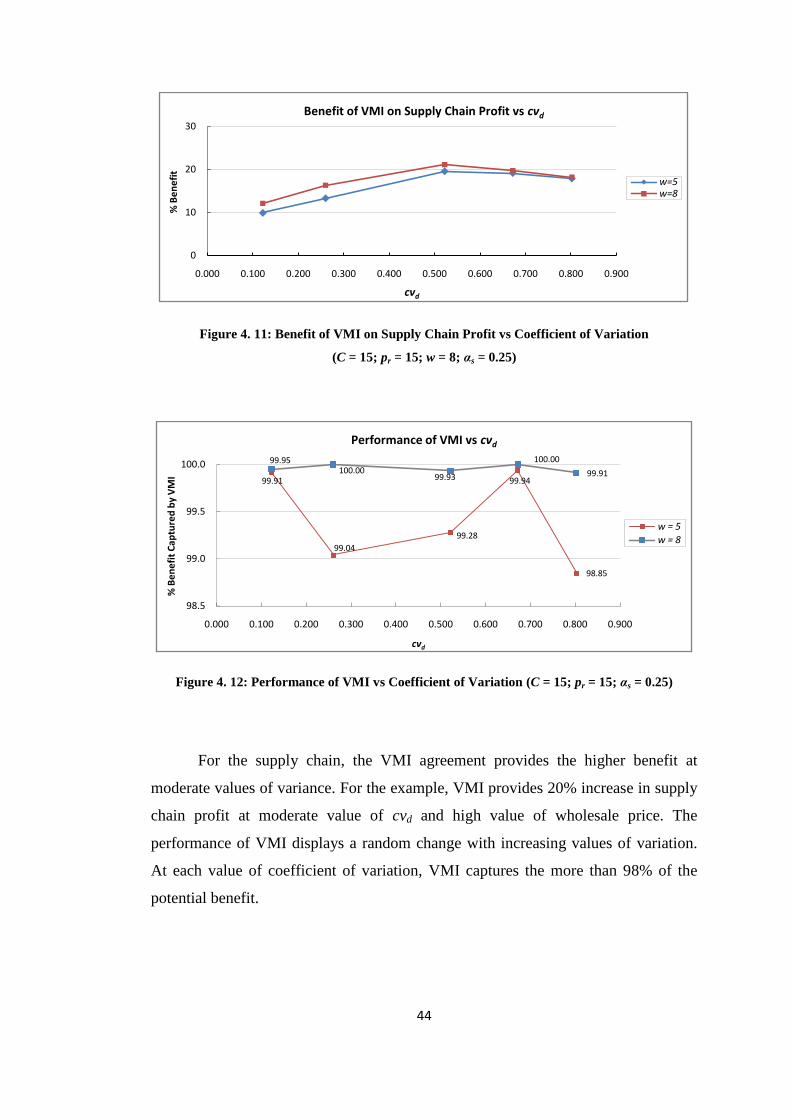
44
Figure 4. 11: Benefit of VMI on Supply Chain Profit vs Coefficient of Variation
(C = 15; pr = 15; w = 8; αs = 0.25)
Figure 4. 12: Performance of VMI vs Coefficient of Variation (C = 15; pr = 15; αs = 0.25)
For the supply chain, the VMI agreement provides the higher benefit at
moderate values of variance. For the example, VMI provides 20% increase in supply
chain profit at moderate value of cvd and high value of wholesale price. The
performance of VMI displays a random change with increasing values of variation.
At each value of coefficient of variation, VMI captures the more than 98% of the
potential benefit.
0
10
20
30
0.000 0.100 0.200 0.300 0.400 0.500 0.600 0.700 0.800 0.900
% B
en
efi
t
cvd
Benefit of VMI on Supply Chain Profit vs cvd
w=5w=8
99.91
99.04
99.28
99.94
98.85
99.95100.00
99.93
100.00
99.91
98.5
99.0
99.5
100.0
0.000 0.100 0.200 0.300 0.400 0.500 0.600 0.700 0.800 0.900
% B
en
efi
t C
aptu
red
by
VM
I
cvd
Performance of VMI vs cvd
w = 5w = 8
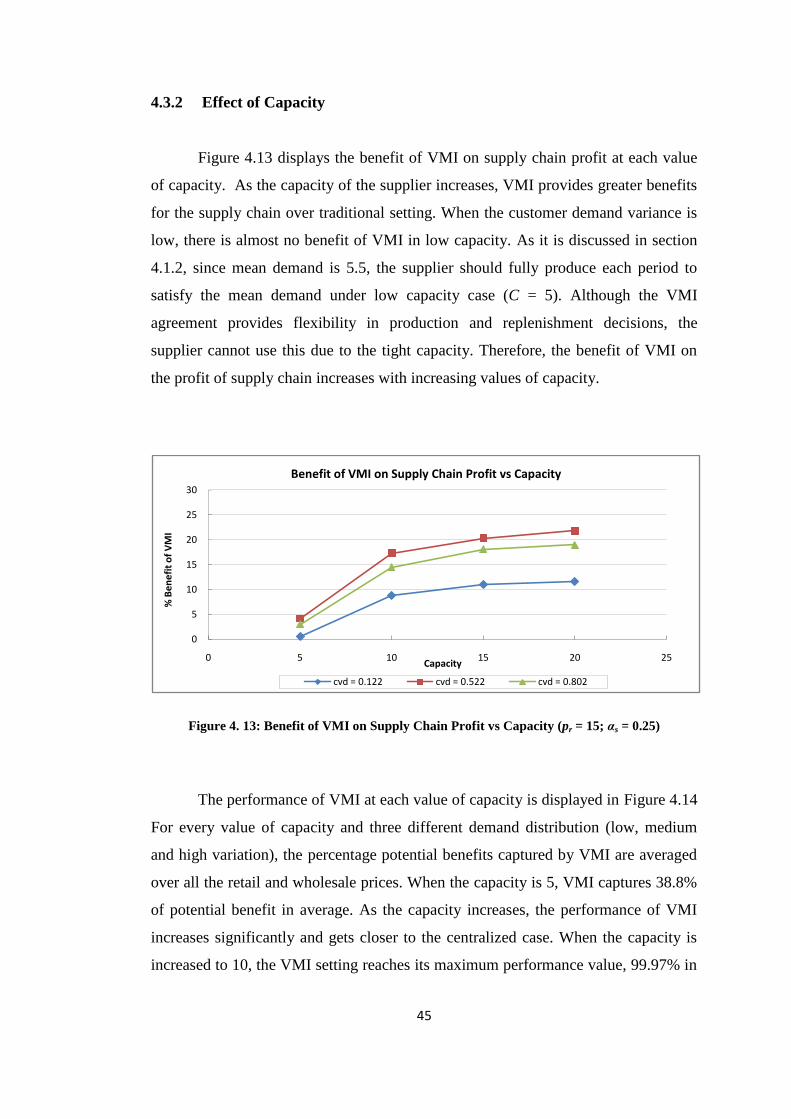
45
4.3.2 Effect of Capacity
Figure 4.13 displays the benefit of VMI on supply chain profit at each value
of capacity. As the capacity of the supplier increases, VMI provides greater benefits
for the supply chain over traditional setting. When the customer demand variance is
low, there is almost no benefit of VMI in low capacity. As it is discussed in section
4.1.2, since mean demand is 5.5, the supplier should fully produce each period to
satisfy the mean demand under low capacity case (C = 5). Although the VMI
agreement provides flexibility in production and replenishment decisions, the
supplier cannot use this due to the tight capacity. Therefore, the benefit of VMI on
the profit of supply chain increases with increasing values of capacity.
Figure 4. 13: Benefit of VMI on Supply Chain Profit vs Capacity (pr = 15; αs = 0.25)
The performance of VMI at each value of capacity is displayed in Figure 4.14
For every value of capacity and three different demand distribution (low, medium
and high variation), the percentage potential benefits captured by VMI are averaged
over all the retail and wholesale prices. When the capacity is 5, VMI captures 38.8%
of potential benefit in average. As the capacity increases, the performance of VMI
increases significantly and gets closer to the centralized case. When the capacity is
increased to 10, the VMI setting reaches its maximum performance value, 99.97% in
0
5
10
15
20
25
30
0 5 10 15 20 25
% B
en
efi
t o
f V
MI
Capacity
Benefit of VMI on Supply Chain Profit vs Capacity
cvd = 0.122 cvd = 0.522 cvd = 0.802
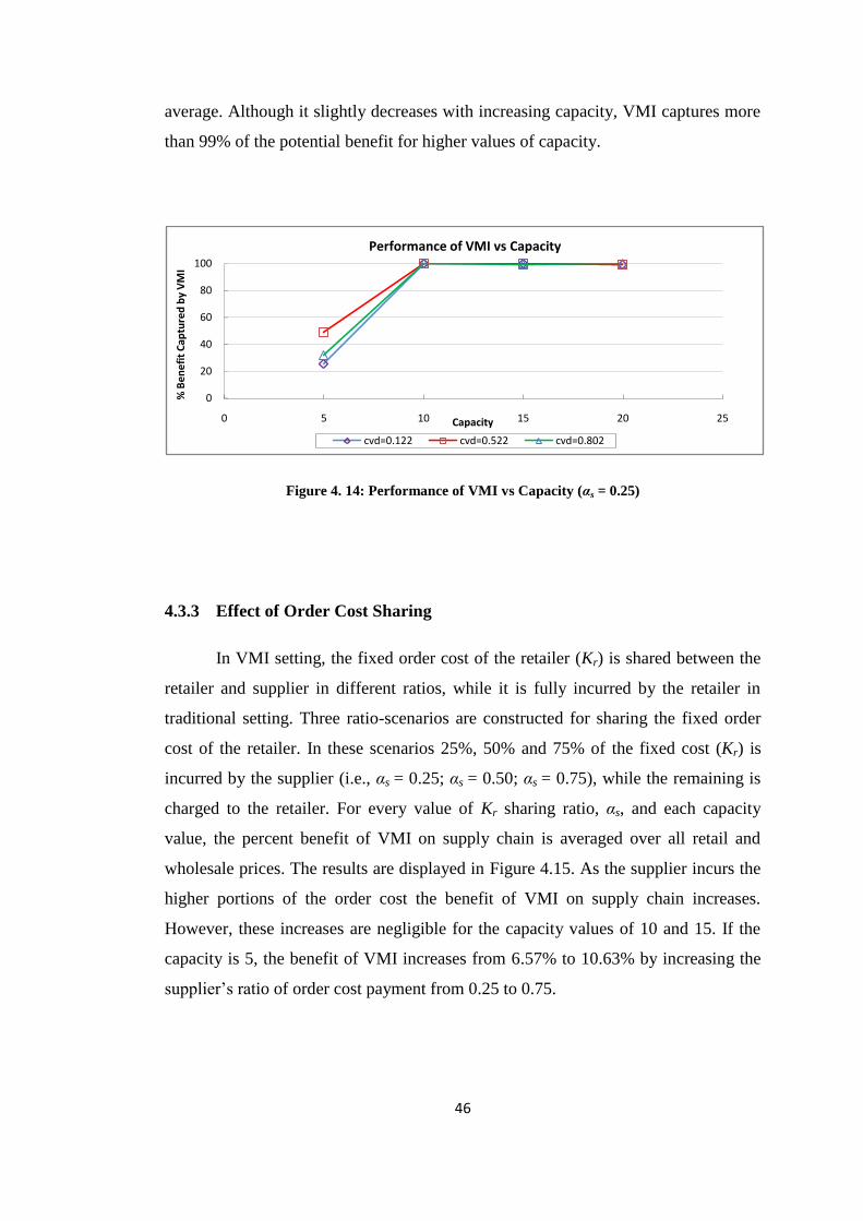
46
average. Although it slightly decreases with increasing capacity, VMI captures more
than 99% of the potential benefit for higher values of capacity.
Figure 4. 14: Performance of VMI vs Capacity (αs = 0.25)
4.3.3 Effect of Order Cost Sharing
In VMI setting, the fixed order cost of the retailer (Kr) is shared between the
retailer and supplier in different ratios, while it is fully incurred by the retailer in
traditional setting. Three ratio-scenarios are constructed for sharing the fixed order
cost of the retailer. In these scenarios 25%, 50% and 75% of the fixed cost (Kr) is
incurred by the supplier (i.e., αs = 0.25; αs = 0.50; αs = 0.75), while the remaining is
charged to the retailer. For every value of Kr sharing ratio, αs, and each capacity
value, the percent benefit of VMI on supply chain is averaged over all retail and
wholesale prices. The results are displayed in Figure 4.15. As the supplier incurs the
higher portions of the order cost the benefit of VMI on supply chain increases.
However, these increases are negligible for the capacity values of 10 and 15. If the
capacity is 5, the benefit of VMI increases from 6.57% to 10.63% by increasing the
supplier‟s ratio of order cost payment from 0.25 to 0.75.
0
20
40
60
80
100
0 5 10 15 20 25
% B
en
efi
t C
aptu
red
by
VM
I
Capacity
Performance of VMI vs Capacity
cvd=0.122 cvd=0.522 cvd=0.802
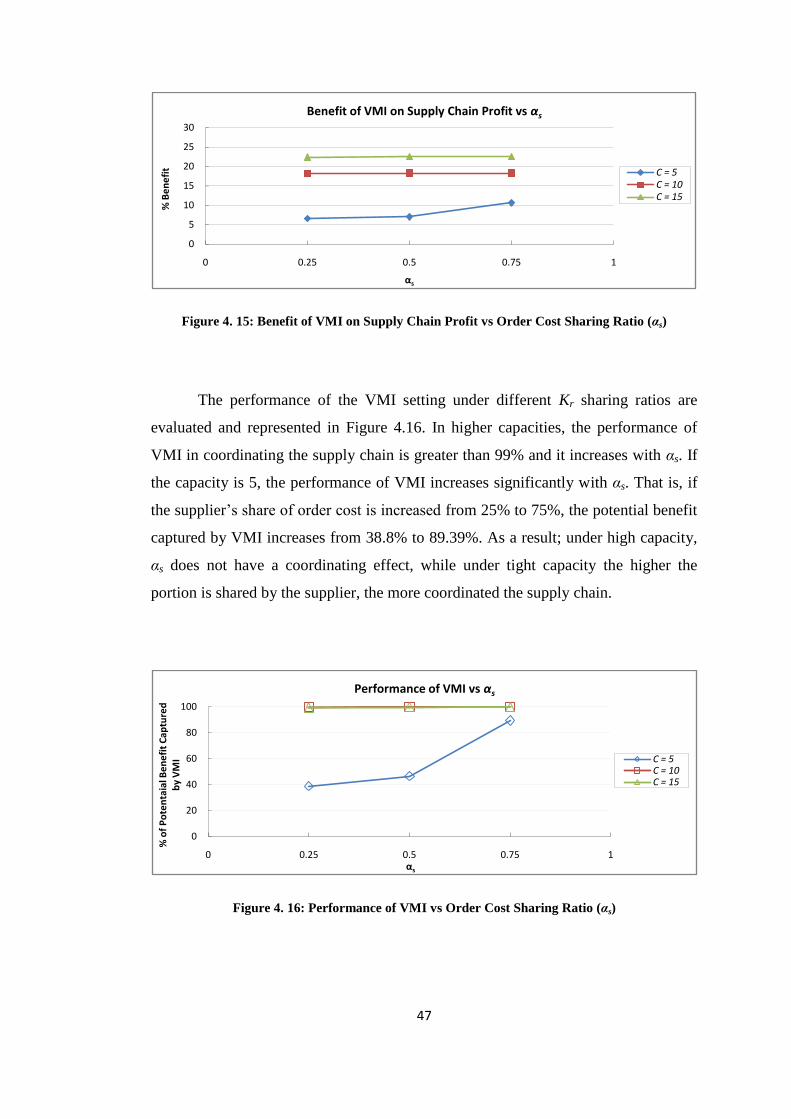
47
Figure 4. 15: Benefit of VMI on Supply Chain Profit vs Order Cost Sharing Ratio (αs)
The performance of the VMI setting under different Kr sharing ratios are
evaluated and represented in Figure 4.16. In higher capacities, the performance of
VMI in coordinating the supply chain is greater than 99% and it increases with αs. If
the capacity is 5, the performance of VMI increases significantly with αs. That is, if
the supplier‟s share of order cost is increased from 25% to 75%, the potential benefit
captured by VMI increases from 38.8% to 89.39%. As a result; under high capacity,
αs does not have a coordinating effect, while under tight capacity the higher the
portion is shared by the supplier, the more coordinated the supply chain.
Figure 4. 16: Performance of VMI vs Order Cost Sharing Ratio (αs)
0
5
10
15
20
25
30
0 0.25 0.5 0.75 1
% B
en
efi
t
αs
Benefit of VMI on Supply Chain Profit vs αs
C = 5C = 10C = 15
0
20
40
60
80
100
0 0.25 0.5 0.75 1
% o
f P
ote
nta
ial B
en
efi
t C
aptu
red
b
y V
MI
αs
Performance of VMI vs αs
C = 5C = 10C = 15
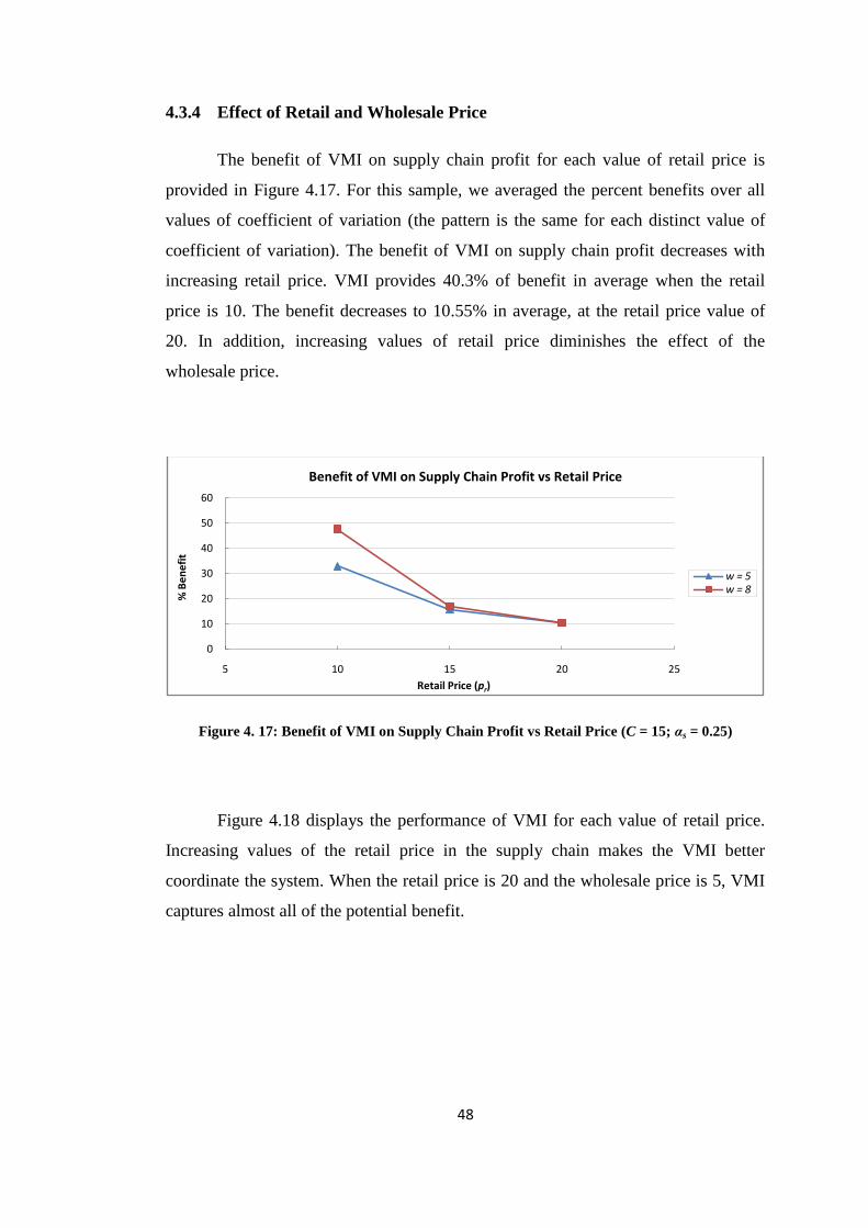
48
4.3.4 Effect of Retail and Wholesale Price
The benefit of VMI on supply chain profit for each value of retail price is
provided in Figure 4.17. For this sample, we averaged the percent benefits over all
values of coefficient of variation (the pattern is the same for each distinct value of
coefficient of variation). The benefit of VMI on supply chain profit decreases with
increasing retail price. VMI provides 40.3% of benefit in average when the retail
price is 10. The benefit decreases to 10.55% in average, at the retail price value of
20. In addition, increasing values of retail price diminishes the effect of the
wholesale price.
Figure 4. 17: Benefit of VMI on Supply Chain Profit vs Retail Price (C = 15; αs = 0.25)
Figure 4.18 displays the performance of VMI for each value of retail price.
Increasing values of the retail price in the supply chain makes the VMI better
coordinate the system. When the retail price is 20 and the wholesale price is 5, VMI
captures almost all of the potential benefit.
0
10
20
30
40
50
60
5 10 15 20 25
% B
en
efi
t
Retail Price (pr)
Benefit of VMI on Supply Chain Profit vs Retail Price
w = 5w = 8
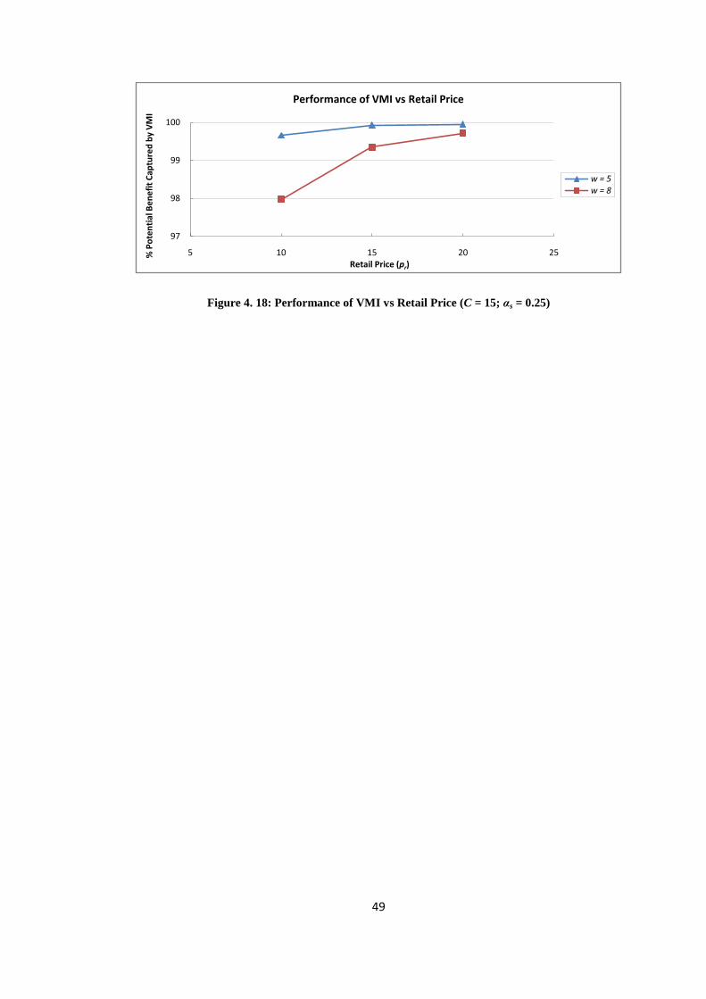
49
Figure 4. 18: Performance of VMI vs Retail Price (C = 15; αs = 0.25)
97
98
99
100
5 10 15 20 25% P
ote
nti
al B
en
efi
t C
aptu
red
by
VM
I
Retail Price (pr)
Performance of VMI vs Retail Price
w = 5w = 8
50
CHAPTER 5
CONCLUSION
In this study, we analyze a VMI system for a supply chain consisting of a
single capacitated supplier and a single retailer. According to the proposed VMI
agreement, the supplier is informed periodically about the inventory level of the
retailer, and she manages the retailer‟s inventory by deciding on the timing and the
quantity of the replenishments on behalf of him. The motivation of the retailer for
participating in such a relationship is provided by transferring some portion of his
fixed ordering cost to the supplier. The replenishments in the VMI setting are forced
to be done according to the (z,Z) policy. That is, the minimum and the maximum
inventory levels, z and Z respectively, are specified in a contract and the supplier
should keep the inventory level of the retailer between these levels. We conduct a
computational study and compare the VMI system with the traditional setting, under
which the supplier has limited (partial) information and the replenishment decision is
made by the retailer himself according to (s,S) policy. The analyses of the benefits
provided by VMI are done from the perspective of the supplier, the retailer and the
overall supply chain. The effects of the capacity, variation of customer demand, retail
price, wholesale price and the order cost sharing ratio to these benefits are analyzed.
VMI system provides significant benefits in many settings, but not for all.
The (z,Z) type of inventory management in the VMI system provides flexibility to
the supplier on the quantity of production and dispatch. However, the utilization of
this flexibility is mainly dependent on the production capacity of the supplier;
therefore the capacity plays an important role on the benefit provided by VMI. When
the capacity of the supplier is low (close to mean demand), the VMI system does not
provide benefit to the supplier, that is, at any (z,Z) level, the supplier cannot get
51
better than traditional setting, although the retailer can. On the other hand, increasing
production capacity yields significant benefits both for the supplier and the retailer.
We analyze the effects of customer demand variability on the benefits. In the
VMI system, as soon as the supplier can utilize the flexibility on dispatch quantity,
her profit does not affected by the customer demand variation in the long-run. VMI
provides the higher benefit for the supplier at moderate or high variation cases,
depending on the retailer‟s policy parameters in the traditional setting. The VMI
system, however, is most beneficial at moderate values of demand variance when we
consider the profit of the retailer and the total supply chain. Under the VMI setting,
the system performs very close to the centralized setting at any value of the demand
variance according to our data set.
Future research can extend the analysis here in many directions. In our supply
chain environment, as soon as the material is shipped to the retailer, the ownership of
the inventory is also transferred to the retailer. A further extension may consider the
consignment stock case under the VMI setting. Another extension could be to aim a
specified service level under the VMI setting.
Finally, one other extension of the study may consider a supply chain
environment with a single supplier who joins in a VMI partnership with two or more
retailers. For such a case, the model we construct for VMI setting can be easily
modified by defining the state with more parameters. However, this case is not
simple to conduct a numerical analysis due to the increased complexity of the model.
52
REFERENCES
Achabal D. Dale, Shelby H. McIntyre, Stephen A. Smith, Kirthi K. (2000). A
decision support system for vendor managed inventory, Journal of Retailing, 76(4),
430-454.
Aviv Y., Federgruen A. (1998). The Operational Benefits of Information
Sharing and Vendor Managed Inventory (VMI) Programs, Working Paper.
Bernstein F., Chen F., Federgruen A. (2006). Coordinating Supply Chains
with Simple Pricing Schemes: The Role of Vendor-Managed Inventories,
Management Science, 52(10), 1483-1492.
Cachon G. P., Fisher M. (2000). Supply Chain Inventory Management and
the Value of Shared Information, Management Science, 46(8), 1032-1048.
Cachon G. (2001). “Stock Wars: Inventory Competition in a Two-echelon
Supply Chain with Multiple Retailers”, Operations Research, 49(5), 658-674.
Cheung K. L., Lee H. L. (2002). The Inventory Benefit of Shipment
Coordination and Stock Rebalancing in a Supply Chain, Management Science, 48(2),
300-306.
Çetinkaya S., Lee C. (2000). Stock Replenishment and Shipment Scheduling
for Vendor-Managed Inventory Systems, Management Science, 46(2), 217-232.
Dong Y., Xu K. (2002). A supply chain model of vendor managed inventory,
Transportation Research Part E: Logistics and Transportation Review, 38(2), 75-95.
Fry M. J., Kapuscinski R., Lennon T. L. (2001). Coordinating Production
and Delivery Under a (z, Z)-Type Vendor-Managed Inventory Contract,
Manufacturing and Service Operations Management, 3(2), 151-173.
Gavirneni S., Kapuscinski R.., Tayur S. (1999). Value of information in
capacitated supply chains, Management Science, 45(1), 16-24.
Gumus M., Jewkes Elizabeth M., Bookbinder James H. (2008). Impact of
consignment inventory and vendor-managed inventory for a two-party supply chain,
International Journal of Production Economics, 113(2), 502-517.
Kleywegt A. J., Nori V. S., Savelsbergh M. W. (2002). The Stochastic
Inventory Routing Problem with Direct Deliveries, Transportation Science, 36(1),
94-118.
53
Valentini G., Zavanella L. (2003). The consignment stock of inventories:
industrial case and performance analysis, International Journal of Production
Economics, 81-82, 215-224.
Waller M., Johnson M. E., Davis T. (1999). Vendor-managed Inventory in
the Retail Supply Chain, Journal of Business Logistics, 20, 183–203.
Yuliang Y., Philip T. Evers, Martin E. Dresner (2007). Supply chain
integration in vendor-managed inventory, Decision Support Systems, 43(2), 663-674.
Zavanella L., Zanoni S. (2009). A one-vendor multi-buyer integrated
production-inventory model: The „Consignment Stock‟ case, International Journal of
Production Economics, 118(1), 225-232.
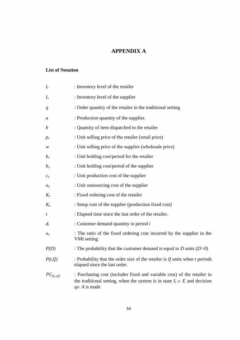
54
APPENDIX A
List of Notation
Ir : Inventory level of the retailer
Is : Inventory level of the supplier
q : Order quantity of the retailer in the traditional setting
a : Production quantity of the supplier.
b : Quantity of item dispatched to the retailer
pr : Unit selling price of the retailer (retail price)
w : Unit selling price of the supplier (wholesale price)
hr : Unit holding cost/period for the retailer
hs : Unit holding cost/period of the supplier
cs : Unit production cost of the supplier
os : Unit outsourcing cost of the supplier
Kr : Fixed ordering cost of the retailer
Ks : Setup cost of the supplier (production fixed cost)
t : Elapsed time since the last order of the retailer.
di : Customer demand quantity in period i
αs : The ratio of the fixed ordering cost incurred by the supplier in the
VMI setting
P(D) : The probability that the customer demand is equal to D units (D>0)
P(t,Q) : Probability that the order size of the retailer is Q units when t periods
elapsed since the last order.
: Purchasing cost (includes fixed and variable cost) of the retailer in
the traditional setting, when the system is in state Ir E and decision
q A is made
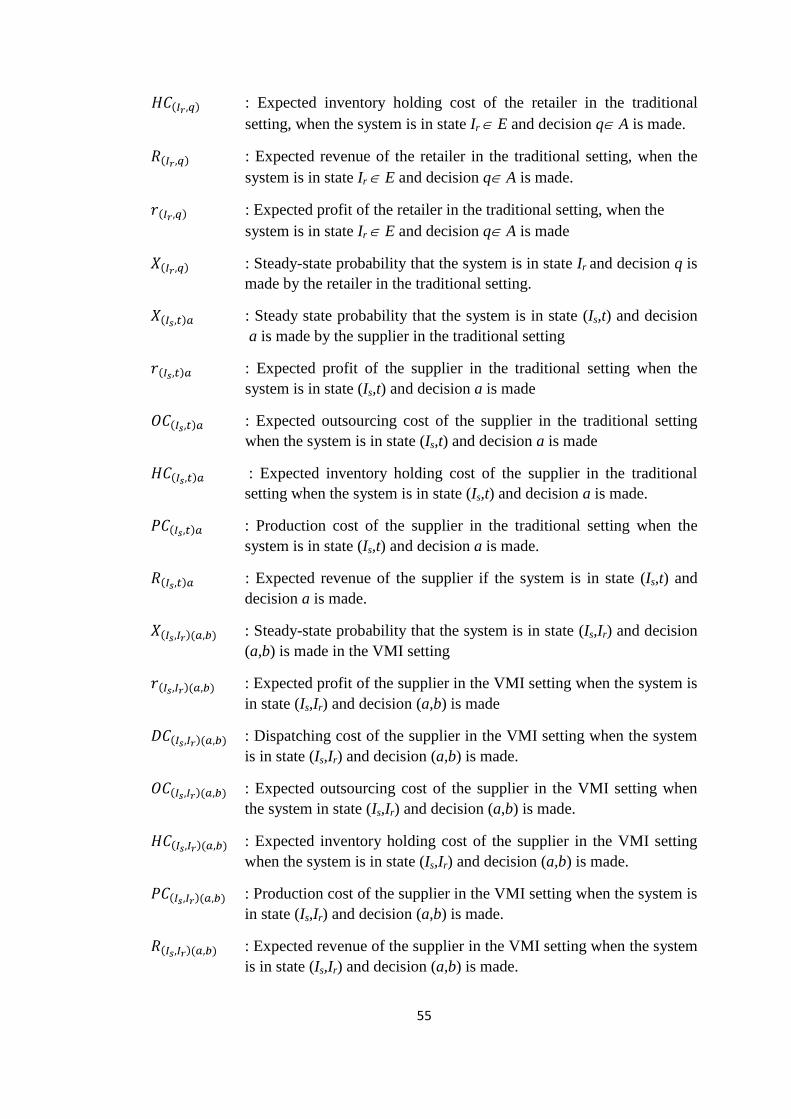
55
: Expected inventory holding cost of the retailer in the traditional
setting, when the system is in state Ir E and decision q A is made.
: Expected revenue of the retailer in the traditional setting, when the
system is in state Ir E and decision q A is made.
: Expected profit of the retailer in the traditional setting, when the
system is in state Ir E and decision q A is made
: Steady-state probability that the system is in state Ir and decision q is
made by the retailer in the traditional setting.
: Steady state probability that the system is in state (Is,t) and decision
a is made by the supplier in the traditional setting
: Expected profit of the supplier in the traditional setting when the
system is in state (Is,t) and decision a is made
: Expected outsourcing cost of the supplier in the traditional setting
when the system is in state (Is,t) and decision a is made
: Expected inventory holding cost of the supplier in the traditional
setting when the system is in state (Is,t) and decision a is made.
: Production cost of the supplier in the traditional setting when the
system is in state (Is,t) and decision a is made.
: Expected revenue of the supplier if the system is in state (Is,t) and
decision a is made.
: Steady-state probability that the system is in state (Is,Ir) and decision
(a,b) is made in the VMI setting
: Expected profit of the supplier in the VMI setting when the system is
in state (Is,Ir) and decision (a,b) is made
: Dispatching cost of the supplier in the VMI setting when the system
is in state (Is,Ir) and decision (a,b) is made.
: Expected outsourcing cost of the supplier in the VMI setting when
the system in state (Is,Ir) and decision (a,b) is made.
: Expected inventory holding cost of the supplier in the VMI setting
when the system is in state (Is,Ir) and decision (a,b) is made.
: Production cost of the supplier in the VMI setting when the system is
in state (Is,Ir) and decision (a,b) is made.
: Expected revenue of the supplier in the VMI setting when the system
is in state (Is,Ir) and decision (a,b) is made.
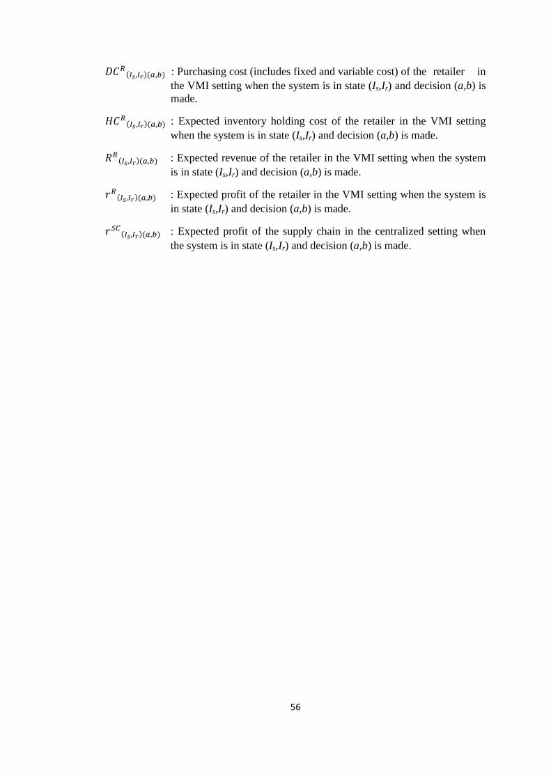
56
: Purchasing cost (includes fixed and variable cost) of the retailer in
the VMI setting when the system is in state (Is,Ir) and decision (a,b) is
made.
: Expected inventory holding cost of the retailer in the VMI setting
when the system is in state (Is,Ir) and decision (a,b) is made.
: Expected revenue of the retailer in the VMI setting when the system
is in state (Is,Ir) and decision (a,b) is made.
: Expected profit of the retailer in the VMI setting when the system is
in state (Is,Ir) and decision (a,b) is made.
: Expected profit of the supply chain in the centralized setting when
the system is in state (Is,Ir) and decision (a,b) is made.
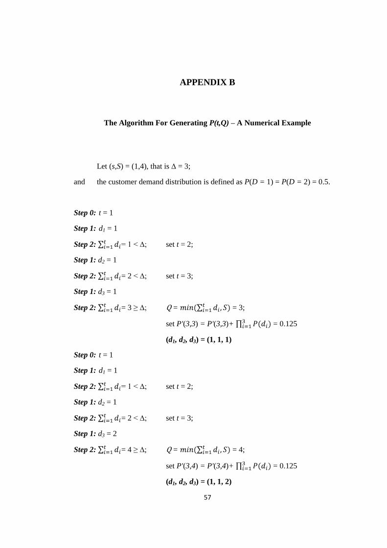
57
APPENDIX B
The Algorithm For Generating P(t,Q) – A Numerical Example
Let (s,S) = (1,4), that is ∆ = 3;
and the customer demand distribution is defined as P(D = 1) = P(D = 2) = 0.5.
Step 0: t = 1
Step 1: d1 = 1
Step 2: = 1 < ∆; set t = 2;
Step 1: d2 = 1
Step 2: = 2 < ∆; set t = 3;
Step 1: d3 = 1
Step 2: = 3 ≥ ∆; Q = = 3;
set P'(3,3) = P'(3,3)+ = 0.125
(d1, d2, d3) = (1, 1, 1)
Step 0: t = 1
Step 1: d1 = 1
Step 2: = 1 < ∆; set t = 2;
Step 1: d2 = 1
Step 2: = 2 < ∆; set t = 3;
Step 1: d3 = 2
Step 2: = 4 ≥ ∆; Q = = 4;
set P'(3,4) = P'(3,4)+ = 0.125
(d1, d2, d3) = (1, 1, 2)
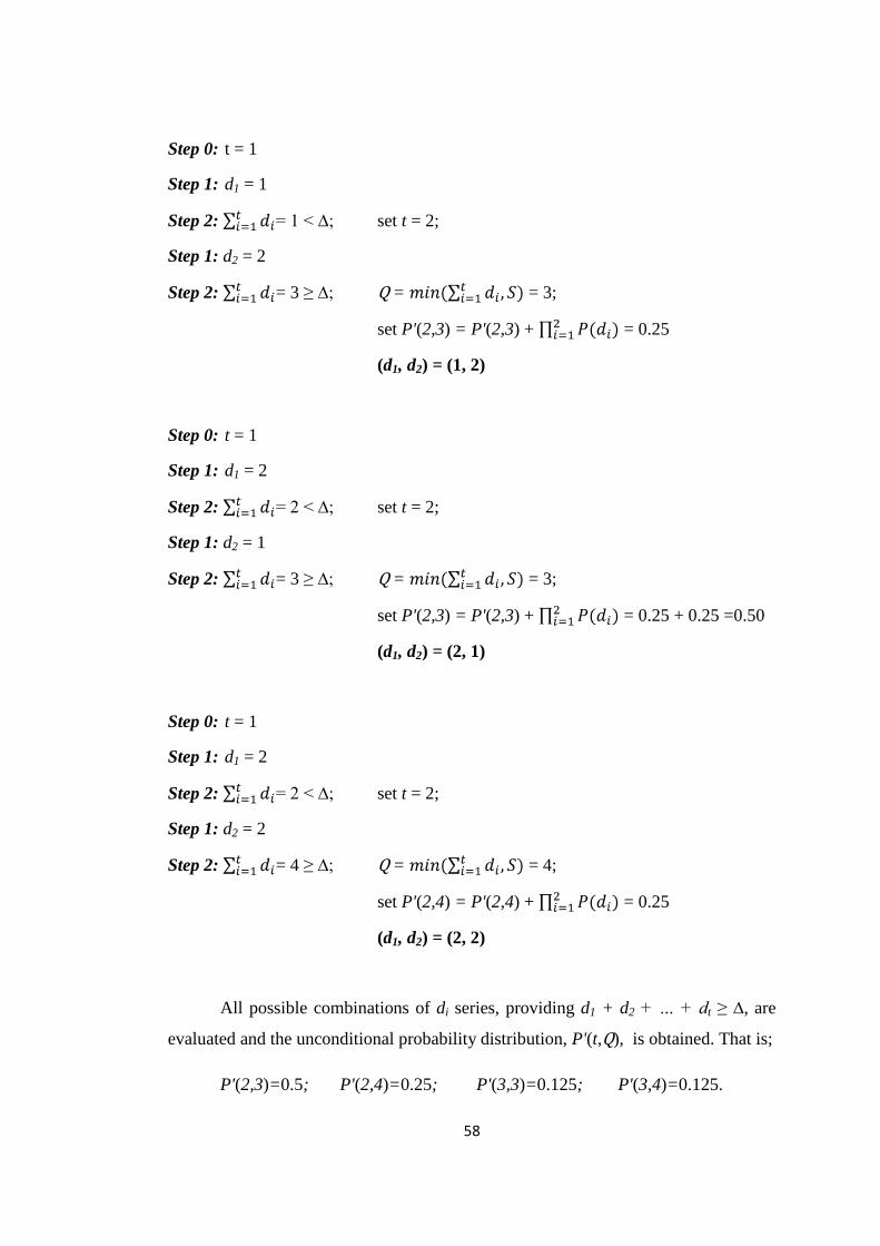
58
Step 0: t = 1
Step 1: d1 = 1
Step 2: = 1 < ∆; set t = 2;
Step 1: d2 = 2
Step 2: = 3 ≥ ∆; Q = = 3;
set P'(2,3) = P'(2,3) + = 0.25
(d1, d2) = (1, 2)
Step 0: t = 1
Step 1: d1 = 2
Step 2: = 2 < ∆; set t = 2;
Step 1: d2 = 1
Step 2: = 3 ≥ ∆; Q = = 3;
set P'(2,3) = P'(2,3) + = 0.25 + 0.25 =0.50
(d1, d2) = (2, 1)
Step 0: t = 1
Step 1: d1 = 2
Step 2: = 2 < ∆; set t = 2;
Step 1: d2 = 2
Step 2: = 4 ≥ ∆; Q = = 4;
set P'(2,4) = P'(2,4) + = 0.25
(d1, d2) = (2, 2)
All possible combinations of di series, providing d1 + d2 + … + dt ≥ ∆, are
evaluated and the unconditional probability distribution, P'(t,Q), is obtained. That is;
P'(2,3)=0.5; P'(2,4)=0.25; P'(3,3)=0.125; P'(3,4)=0.125.
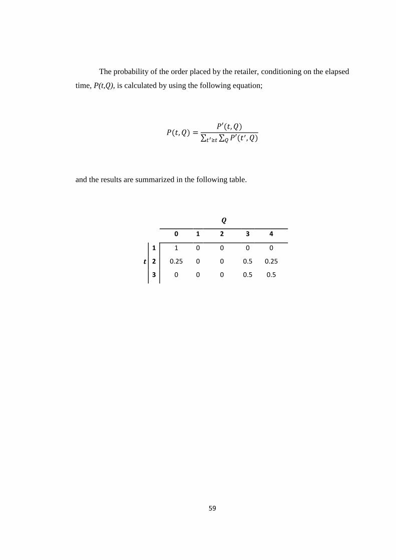
59
The probability of the order placed by the retailer, conditioning on the elapsed
time, P(t,Q), is calculated by using the following equation;
and the results are summarized in the following table.
Q
0 1 2 3 4
t
1 1 0 0 0 0
2 0.25 0 0 0.5 0.25
3 0 0 0 0.5 0.5
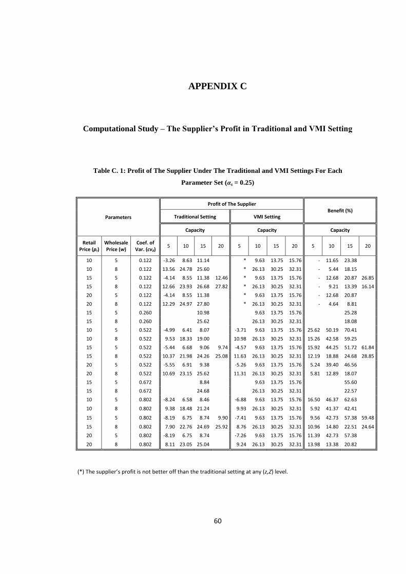
60
APPENDIX C
Computational Study – The Supplier’s Profit in Traditional and VMI Setting
Table C. 1: Profit of The Supplier Under The Traditional and VMI Settings For Each
Parameter Set (αs = 0.25)
Parameters
Profit of The Supplier Benefit (%)
Traditional Setting VMI Setting
Capacity Capacity Capacity
Retail Price (pr)
Wholesale Price (w)
Coef. of Var. (cvd)
5 10 15 20 5 10 15 20 5 10 15 20
10 5 0.122 -3.26 8.63 11.14 * 9.63 13.75 15.76 - 11.65 23.38
10 8 0.122 13.56 24.78 25.60
* 26.13 30.25 32.31 - 5.44 18.15
15 5 0.122 -4.14 8.55 11.38 12.46 * 9.63 13.75 15.76 - 12.68 20.87 26.85
15 8 0.122 12.66 23.93 26.68 27.82 * 26.13 30.25 32.31 - 9.21 13.39 16.14
20 5 0.122 -4.14 8.55 11.38
* 9.63 13.75 15.76 - 12.68 20.87
20 8 0.122 12.29 24.97 27.80 * 26.13 30.25 32.31 - 4.64 8.81
15 5 0.260
10.98
9.63 13.75 15.76
25.28
15 8 0.260
25.62
26.13 30.25 32.31
18.08
10 5 0.522 -4.99 6.41 8.07 -3.71 9.63 13.75 15.76 25.62 50.19 70.41
10 8 0.522 9.53 18.33 19.00
10.98 26.13 30.25 32.31 15.26 42.58 59.25
15 5 0.522 -5.44 6.68 9.06 9.74 -4.57 9.63 13.75 15.76 15.92 44.25 51.72 61.84
15 8 0.522 10.37 21.98 24.26 25.08 11.63 26.13 30.25 32.31 12.19 18.88 24.68 28.85
20 5 0.522 -5.55 6.91 9.38
-5.26 9.63 13.75 15.76 5.24 39.40 46.56
20 8 0.522 10.69 23.15 25.62
11.31 26.13 30.25 32.31 5.81 12.89 18.07
15 5 0.672
8.84
9.63 13.75 15.76
55.60
15 8 0.672
24.68
26.13 30.25 32.31
22.57
10 5 0.802 -8.24 6.58 8.46
-6.88 9.63 13.75 15.76 16.50 46.37 62.63
10 8 0.802 9.38 18.48 21.24
9.93 26.13 30.25 32.31 5.92 41.37 42.41
15 5 0.802 -8.19 6.75 8.74 9.90 -7.41 9.63 13.75 15.76 9.56 42.73 57.38 59.48
15 8 0.802 7.90 22.76 24.69 25.92 8.76 26.13 30.25 32.31 10.96 14.80 22.51 24.64
20 5 0.802 -8.19 6.75 8.74
-7.26 9.63 13.75 15.76 11.39 42.73 57.38
20 8 0.802 8.11 23.05 25.04 9.24 26.13 30.25 32.31 13.98 13.38 20.82
(*) The supplier’s profit is not better off than the traditional setting at any (z,Z) level.
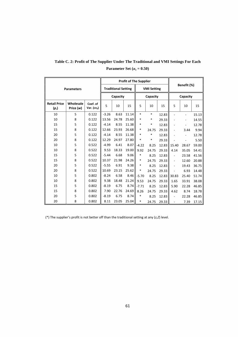
61
Table C. 2: Profit of The Supplier Under The Traditional and VMI Settings For Each
Parameter Set (αs = 0.50)
Parameters
Profit of The Supplier Benefit (%)
Traditional Setting VMI Setting
Capacity Capacity Capacity
Retail Price (pr)
Wholesale Price (w)
Coef. of Var. (cvd)
5 10 15 5 10 15 5 10 15
10 5 0.122 -3.26 8.63 11.14 * * 12.83 - - 15.13
10 8 0.122 13.56 24.78 25.60 * * 29.33 - - 14.55
15 5 0.122 -4.14 8.55 11.38 * * 12.83 - - 12.78
15 8 0.122 12.66 23.93 26.68 * 24.75 29.33 - 3.44 9.94
20 5 0.122 -4.14 8.55 11.38 * * 12.83 - - 12.78
20 8 0.122 12.29 24.97 27.80 * * 29.33 - - 5.50
10 5 0.522 -4.99 6.41 8.07 -4.22 8.25 12.83 15.40 28.67 59.00
10 8 0.522 9.53 18.33 19.00 9.92 24.75 29.33 4.14 35.05 54.41
15 5 0.522 -5.44 6.68 9.06 * 8.25 12.83 - 23.58 41.56
15 8 0.522 10.37 21.98 24.26 * 24.75 29.33 - 12.60 20.88
20 5 0.522 -5.55 6.91 9.38 * 8.25 12.83 - 19.43 36.75
20 8 0.522 10.69 23.15 25.62 * 24.75 29.33 - 6.93 14.48
10 5 0.802 -8.24 6.58 8.46 -5.70 8.25 12.83 30.83 25.40 51.74
10 8 0.802 9.38 18.48 21.24 9.53 24.75 29.33 1.65 33.91 38.08
15 5 0.802 -8.19 6.75 8.74 -7.71 8.25 12.83 5.90 22.28 46.85
15 8 0.802 7.90 22.76 24.69 8.26 24.75 29.33 4.62 8.74 18.78
20 5 0.802 -8.19 6.75 8.74 * 8.25 12.83 - 22.28 46.85
20 8 0.802 8.11 23.05 25.04 * 24.75 29.33 - 7.39 17.15
(*) The supplier’s profit is not better off than the traditional setting at any (z,Z) level.
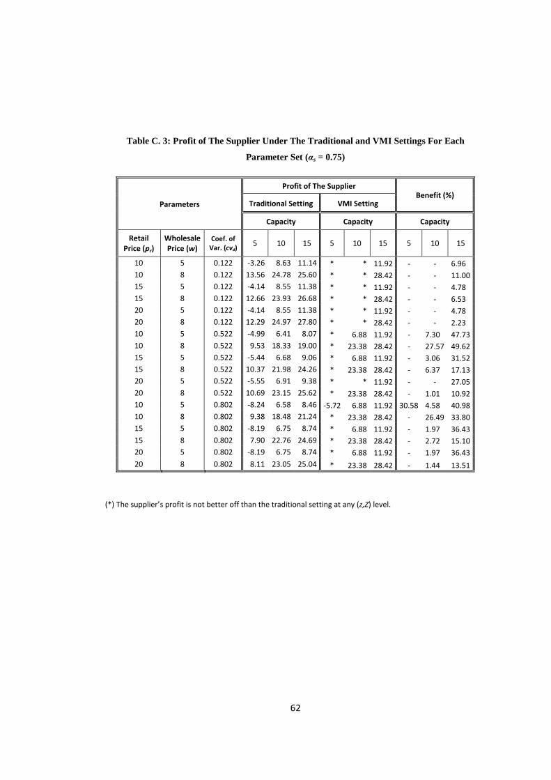
62
Table C. 3: Profit of The Supplier Under The Traditional and VMI Settings For Each
Parameter Set (αs = 0.75)
Parameters
Profit of The Supplier Benefit (%)
Traditional Setting VMI Setting
Capacity Capacity Capacity
Retail Price (pr)
Wholesale Price (w)
Coef. of Var. (cvd)
5 10 15 5 10 15 5 10 15
10 5 0.122 -3.26 8.63 11.14 * * 11.92 - - 6.96
10 8 0.122 13.56 24.78 25.60 * * 28.42 - - 11.00
15 5 0.122 -4.14 8.55 11.38 * * 11.92 - - 4.78
15 8 0.122 12.66 23.93 26.68 * * 28.42 - - 6.53
20 5 0.122 -4.14 8.55 11.38 * * 11.92 - - 4.78
20 8 0.122 12.29 24.97 27.80 * * 28.42 - - 2.23
10 5 0.522 -4.99 6.41 8.07 * 6.88 11.92 - 7.30 47.73
10 8 0.522 9.53 18.33 19.00 * 23.38 28.42 - 27.57 49.62
15 5 0.522 -5.44 6.68 9.06 * 6.88 11.92 - 3.06 31.52
15 8 0.522 10.37 21.98 24.26 * 23.38 28.42 - 6.37 17.13
20 5 0.522 -5.55 6.91 9.38 * * 11.92 - - 27.05
20 8 0.522 10.69 23.15 25.62 * 23.38 28.42 - 1.01 10.92
10 5 0.802 -8.24 6.58 8.46 -5.72 6.88 11.92 30.58 4.58 40.98
10 8 0.802 9.38 18.48 21.24 * 23.38 28.42 - 26.49 33.80
15 5 0.802 -8.19 6.75 8.74 * 6.88 11.92 - 1.97 36.43
15 8 0.802 7.90 22.76 24.69 * 23.38 28.42 - 2.72 15.10
20 5 0.802 -8.19 6.75 8.74 * 6.88 11.92 - 1.97 36.43
20 8 0.802 8.11 23.05 25.04 * 23.38 28.42 - 1.44 13.51
(*) The supplier’s profit is not better off than the traditional setting at any (z,Z) level.
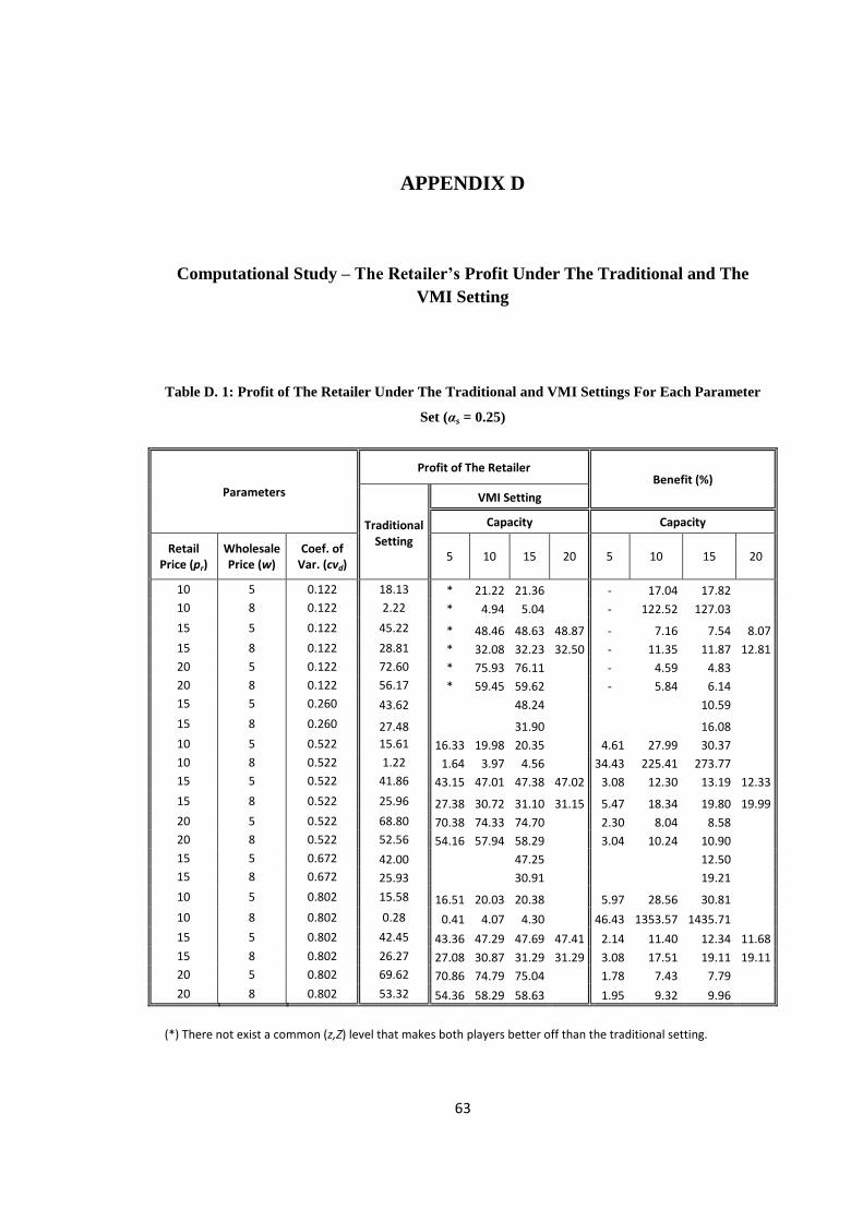
63
APPENDIX D
Computational Study – The Retailer’s Profit Under The Traditional and The
VMI Setting
Table D. 1: Profit of The Retailer Under The Traditional and VMI Settings For Each Parameter
Set (αs = 0.25)
Parameters
Profit of The Retailer Benefit (%)
Traditional Setting
VMI Setting
Capacity Capacity
Retail Price (pr)
Wholesale Price (w)
Coef. of Var. (cvd)
5 10 15 20 5 10 15 20
10 5 0.122 18.13 * 21.22 21.36 - 17.04 17.82
10 8 0.122 2.22 * 4.94 5.04 - 122.52 127.03
15 5 0.122 45.22 * 48.46 48.63 48.87 - 7.16 7.54 8.07
15 8 0.122 28.81 * 32.08 32.23 32.50 - 11.35 11.87 12.81
20 5 0.122 72.60 * 75.93 76.11 - 4.59 4.83
20 8 0.122 56.17 * 59.45 59.62 - 5.84 6.14
15 5 0.260 43.62
48.24
10.59
15 8 0.260 27.48
31.90
16.08
10 5 0.522 15.61 16.33 19.98 20.35 4.61 27.99 30.37
10 8 0.522 1.22 1.64 3.97 4.56 34.43 225.41 273.77
15 5 0.522 41.86 43.15 47.01 47.38 47.02 3.08 12.30 13.19 12.33
15 8 0.522 25.96 27.38 30.72 31.10 31.15 5.47 18.34 19.80 19.99
20 5 0.522 68.80 70.38 74.33 74.70 2.30 8.04 8.58
20 8 0.522 52.56 54.16 57.94 58.29 3.04 10.24 10.90
15 5 0.672 42.00
47.25
12.50
15 8 0.672 25.93
30.91
19.21
10 5 0.802 15.58 16.51 20.03 20.38 5.97 28.56 30.81
10 8 0.802 0.28 0.41 4.07 4.30 46.43 1353.57 1435.71
15 5 0.802 42.45 43.36 47.29 47.69 47.41 2.14 11.40 12.34 11.68
15 8 0.802 26.27 27.08 30.87 31.29 31.29 3.08 17.51 19.11 19.11
20 5 0.802 69.62 70.86 74.79 75.04 1.78 7.43 7.79
20 8 0.802 53.32 54.36 58.29 58.63 1.95 9.32 9.96
(*) There not exist a common (z,Z) level that makes both players better off than the traditional setting.
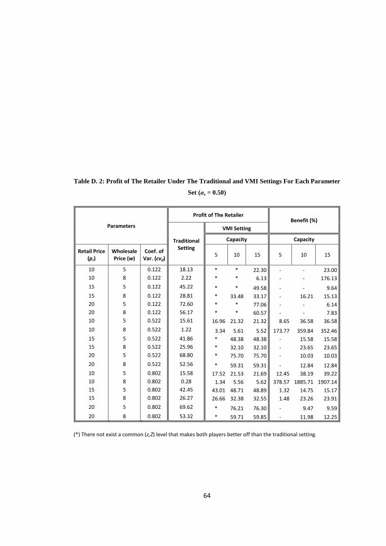
64
Table D. 2: Profit of The Retailer Under The Traditional and VMI Settings For Each Parameter
Set (αs = 0.50)
Parameters
Profit of The Retailer Benefit (%)
Traditional Setting
VMI Setting
Capacity Capacity
Retail Price (pr)
Wholesale Price (w)
Coef. of Var. (cvd)
5 10 15 5 10 15
10 5 0.122 18.13 * * 22.30 - - 23.00
10 8 0.122 2.22 * * 6.13 - - 176.13
15 5 0.122 45.22 * * 49.58 - - 9.64
15 8 0.122 28.81 * 33.48 33.17 - 16.21 15.13
20 5 0.122 72.60 * * 77.06 - - 6.14
20 8 0.122 56.17 * * 60.57 - - 7.83
10 5 0.522 15.61 16.96 21.32 21.32 8.65 36.58 36.58
10 8 0.522 1.22 3.34 5.61 5.52 173.77 359.84 352.46
15 5 0.522 41.86 * 48.38 48.38 - 15.58 15.58
15 8 0.522 25.96 * 32.10 32.10 - 23.65 23.65
20 5 0.522 68.80 * 75.70 75.70 - 10.03 10.03
20 8 0.522 52.56 * 59.31 59.31 - 12.84 12.84
10 5 0.802 15.58 17.52 21.53 21.69 12.45 38.19 39.22
10 8 0.802 0.28 1.34 5.56 5.62 378.57 1885.71 1907.14
15 5 0.802 42.45 43.01 48.71 48.89 1.32 14.75 15.17
15 8 0.802 26.27 26.66 32.38 32.55 1.48 23.26 23.91
20 5 0.802 69.62 * 76.21 76.30 - 9.47 9.59
20 8 0.802 53.32 * 59.71 59.85 - 11.98 12.25
(*) There not exist a common (z,Z) level that makes both players better off than the traditional setting.
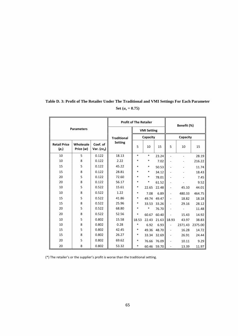
65
Table D. 3: Profit of The Retailer Under The Traditional and VMI Settings For Each Parameter
Set (αs = 0.75)
Parameters
Profit of The Retailer Benefit (%)
Traditional Setting
VMI Setting
Capacity Capacity
Retail Price (pr)
Wholesale Price (w)
Coef. of Var. (cvd)
5 10 15 5 10 15
10 5 0.122 18.13 * * 23.24 - - 28.19
10 8 0.122 2.22 * * 7.02 - - 216.22
15 5 0.122 45.22 * * 50.53 - - 11.74
15 8 0.122 28.81 * * 34.12 - - 18.43
20 5 0.122 72.60 * * 78.01 - - 7.45
20 8 0.122 56.17 * * 61.52 - - 9.52
10 5 0.522 15.61 * 22.65 22.48 - 45.10 44.01
10 8 0.522 1.22 * 7.08 6.89 - 480.33 464.75
15 5 0.522 41.86 * 49.74 49.47 - 18.82 18.18
15 8 0.522 25.96 * 33.53 33.26 - 29.16 28.12
20 5 0.522 68.80 * * 76.70 - - 11.48
20 8 0.522 52.56 * 60.67 60.40 - 15.43 14.92
10 5 0.802 15.58 18.53 22.43 21.63 18.93 43.97 38.83
10 8 0.802 0.28 * 6.92 6.93 - 2371.43 2375.00
15 5 0.802 42.45 * 49.36 48.70 - 16.28 14.72
15 8 0.802 26.27 * 33.34 32.69 - 26.91 24.44
20 5 0.802 69.62 * 76.66 76.09 - 10.11 9.29
20 8 0.802 53.32 * 60.46 59.70 - 13.39 11.97
(*) The retailer’s or the supplier’s profit is worse than the traditional setting.
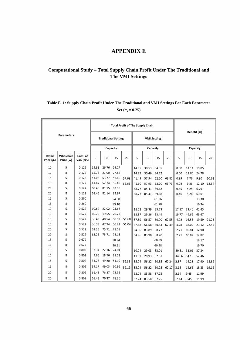
66
APPENDIX E
Computational Study – Total Supply Chain Profit Under The Traditional and
The VMI Settings
Table E. 1: Supply Chain Profit Under The Traditional and VMI Settings For Each Parameter
Set (αs = 0.25)
Parameters
Total Profit of The Supply Chain
Benefit (%)
Traditional Setting VMI Setting
Capacity Capacity Capacity
Retail Price (pr)
Wholesale Price (w)
Coef. of Var. (cvd)
5 10 15 20 5 10 15 20 5 10 15 20
10 5 0.122 14.88 26.76 29.27 14.95 30.53 34.85 0.50 14.11 19.05
10 8 0.122 15.78 27.00 27.82 14.95 30.46 34.72 0.00 12.80 24.78
15 5 0.122 41.08 53.77 56.60 57.68 41.49 57.94 62.20 63.81 0.99 7.76 9.90 10.62
15 8 0.122 41.47 52.74 55.49 56.63 41.50 57.93 62.20 63.73 0.08 9.85 12.10 12.54
20 5 0.122 68.46 81.15 83.98 68.77 85.41 89.68 0.45 5.25 6.79
20 8 0.122 68.46 81.14 83.97 68.77 85.41 89.68 0.46 5.26 6.80
15 5 0.260
54.60
61.86
13.30
15 8 0.260
53.10
61.78
16.34
10 5 0.522 10.62 22.02 23.68
12.52 29.39 33.73 17.87 33.46 42.45
10 8 0.522 10.75 19.55 20.22
12.87 29.26 33.49 19.77 49.69 65.67
15 5 0.522 36.43 48.54 50.92 51.60 37.89 56.57 60.90 62.55 4.02 16.55 19.59 21.23
15 8 0.522 36.33 47.94 50.22 51.04 37.88 56.58 60.83 62.49 4.28 18.02 21.12 22.45
20 5 0.522 63.25 75.71 78.18
64.96 83.89 88.27 2.71 10.81 12.90
20 8 0.522 63.25 75.71 78.18
64.96 83.90 88.20 2.71 10.82 12.82
15 5 0.672
50.84
60.59
19.17
15 8 0.672
50.61
60.58
19.70
10 5 0.802 7.34 22.16 24.04 10.24 29.03 33.01 39.51 31.01 37.34
10 8 0.802 9.66 18.76 21.52 11.07 28.93 32.81 14.66 54.19 52.46
15 5 0.802 34.26 49.20 51.19 52.35 35.24 56.22 60.35 62.24 2.87 14.28 17.90 18.89
15 8 0.802 34.17 49.03 50.96 52.19 35.24 56.22 60.25 62.17 3.15 14.66 18.23 19.12
20 5 0.802 61.43 76.37 78.36 62.74 83.58 87.75 2.14 9.45 11.99
20 8 0.802 61.43 76.37 78.36 62.74 83.58 87.75 2.14 9.45 11.99
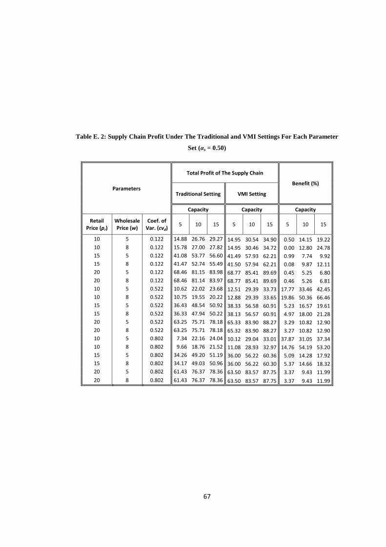
67
Table E. 2: Supply Chain Profit Under The Traditional and VMI Settings For Each Parameter
Set (αs = 0.50)
Parameters
Total Profit of The Supply Chain
Benefit (%)
Traditional Setting VMI Setting
Capacity Capacity Capacity
Retail Price (pr)
Wholesale Price (w)
Coef. of Var. (cvd)
5 10 15 5 10 15 5 10 15
10 5 0.122 14.88 26.76 29.27 14.95 30.54 34.90 0.50 14.15 19.22
10 8 0.122 15.78 27.00 27.82 14.95 30.46 34.72 0.00 12.80 24.78
15 5 0.122 41.08 53.77 56.60 41.49 57.93 62.21 0.99 7.74 9.92
15 8 0.122 41.47 52.74 55.49 41.50 57.94 62.21 0.08 9.87 12.11
20 5 0.122 68.46 81.15 83.98 68.77 85.41 89.69 0.45 5.25 6.80
20 8 0.122 68.46 81.14 83.97 68.77 85.41 89.69 0.46 5.26 6.81
10 5 0.522 10.62 22.02 23.68 12.51 29.39 33.73 17.77 33.46 42.45
10 8 0.522 10.75 19.55 20.22 12.88 29.39 33.65 19.86 50.36 66.46
15 5 0.522 36.43 48.54 50.92 38.33 56.58 60.91 5.23 16.57 19.61
15 8 0.522 36.33 47.94 50.22 38.13 56.57 60.91 4.97 18.00 21.28
20 5 0.522 63.25 75.71 78.18 65.33 83.90 88.27 3.29 10.82 12.90
20 8 0.522 63.25 75.71 78.18 65.32 83.90 88.27 3.27 10.82 12.90
10 5 0.802 7.34 22.16 24.04 10.12 29.04 33.01 37.87 31.05 37.34
10 8 0.802 9.66 18.76 21.52 11.08 28.93 32.97 14.76 54.19 53.20
15 5 0.802 34.26 49.20 51.19 36.00 56.22 60.36 5.09 14.28 17.92
15 8 0.802 34.17 49.03 50.96 36.00 56.22 60.30 5.37 14.66 18.32
20 5 0.802 61.43 76.37 78.36 63.50 83.57 87.75 3.37 9.43 11.99
20 8 0.802 61.43 76.37 78.36 63.50 83.57 87.75 3.37 9.43 11.99
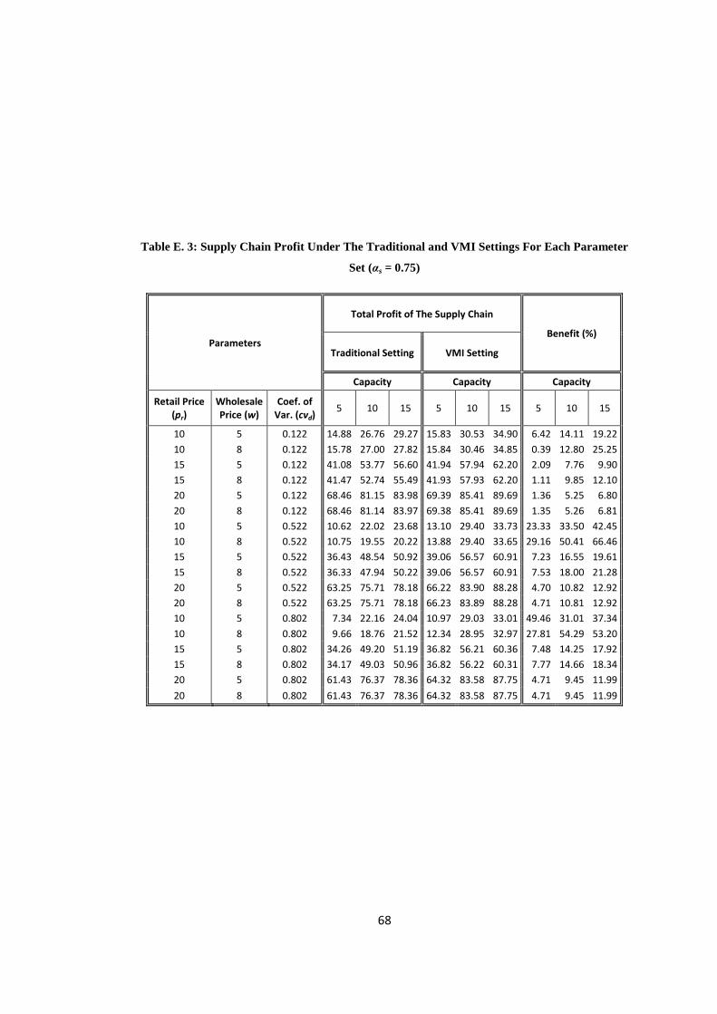
68
Table E. 3: Supply Chain Profit Under The Traditional and VMI Settings For Each Parameter
Set (αs = 0.75)
Parameters
Total Profit of The Supply Chain
Benefit (%)
Traditional Setting VMI Setting
Capacity Capacity Capacity
Retail Price (pr)
Wholesale Price (w)
Coef. of Var. (cvd)
5 10 15 5 10 15 5 10 15
10 5 0.122 14.88 26.76 29.27 15.83 30.53 34.90 6.42 14.11 19.22
10 8 0.122 15.78 27.00 27.82 15.84 30.46 34.85 0.39 12.80 25.25
15 5 0.122 41.08 53.77 56.60 41.94 57.94 62.20 2.09 7.76 9.90
15 8 0.122 41.47 52.74 55.49 41.93 57.93 62.20 1.11 9.85 12.10
20 5 0.122 68.46 81.15 83.98 69.39 85.41 89.69 1.36 5.25 6.80
20 8 0.122 68.46 81.14 83.97 69.38 85.41 89.69 1.35 5.26 6.81
10 5 0.522 10.62 22.02 23.68 13.10 29.40 33.73 23.33 33.50 42.45
10 8 0.522 10.75 19.55 20.22 13.88 29.40 33.65 29.16 50.41 66.46
15 5 0.522 36.43 48.54 50.92 39.06 56.57 60.91 7.23 16.55 19.61
15 8 0.522 36.33 47.94 50.22 39.06 56.57 60.91 7.53 18.00 21.28
20 5 0.522 63.25 75.71 78.18 66.22 83.90 88.28 4.70 10.82 12.92
20 8 0.522 63.25 75.71 78.18 66.23 83.89 88.28 4.71 10.81 12.92
10 5 0.802 7.34 22.16 24.04 10.97 29.03 33.01 49.46 31.01 37.34
10 8 0.802 9.66 18.76 21.52 12.34 28.95 32.97 27.81 54.29 53.20
15 5 0.802 34.26 49.20 51.19 36.82 56.21 60.36 7.48 14.25 17.92
15 8 0.802 34.17 49.03 50.96 36.82 56.22 60.31 7.77 14.66 18.34
20 5 0.802 61.43 76.37 78.36 64.32 83.58 87.75 4.71 9.45 11.99
20 8 0.802 61.43 76.37 78.36 64.32 83.58 87.75 4.71 9.45 11.99