Introduction to Weather Derivatives - hu- · PDF fileIntroduction to Weather Derivatives ......
39
Introduction to Weather Derivatives Brenda L´ opez Cabrera Wolfgang K. H¨ ardle CASE-Center for Applied Statistics and Economics Humboldt-Universit¨ at zu Berlin
-
Upload
nguyennguyet -
Category
Documents
-
view
225 -
download
2
Transcript of Introduction to Weather Derivatives - hu- · PDF fileIntroduction to Weather Derivatives ......

Introduction to Weather Derivatives
Brenda Lopez CabreraWolfgang K. Hardle
CASE-Center for Applied Statistics andEconomicsHumboldt-Universitat zu Berlin
1
�
Motivation 1-1
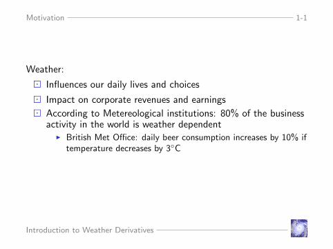
Weather:
� Influences our daily lives and choices
� Impact on corporate revenues and earnings
� According to Metereological institutions: 80% of the businessactivity in the world is weather dependent
I British Met Office: daily beer consumption increases by 10% iftemperature decreases by 3◦C
Introduction to Weather Derivatives

Motivation 1-2
� Climate changes related ”El Nino”
� Global climate changes the volatility of weather
� The occurrence of extreme weather events increases
� Emergence of international weather markets new opportunitiesarise to handle these risks
I Weather Derivatives (WD)
Introduction to Weather Derivatives
Motivation 1-3
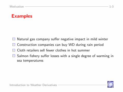
Examples
� Natural gas company suffer negative impact in mild winter
� Construction companies can buy WD during rain period
� Cloth retailers sell fewer clothes in hot summer
� Salmon fishery suffer losses with a single degree of warming insea temperatures
Introduction to Weather Derivatives
Outline 2-1
Outline
1. Motivation X
2. What are Weather Derivatives?
3. Weather Indices
4. Valuation of Weather Derivatives
5. Application
Introduction to Weather Derivatives
What are Weather Derivatives (WD)? 3-1
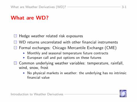
What are WD?
� Hedge weather related risk exposures
� WD returns uncorrelated with other financial instruments
� Formal exchanges: Chicago Mercantile Exchange (CME)I Monthly and seasonal temperature future contractsI European call and put options on these futures
� Common underlying weather variables: temperature, rainfall,wind, snow, frost
I No physical markets in weather: the underlying has no intrinsicfinancial value
Introduction to Weather Derivatives

What are Weather Derivatives (WD)? 3-2
Anatomy of a WD
A weather derivative is defined by several elements:
� Reference Weather Station
� Index
� Term
� Structure: puts, calls, swaps, collars, straddles, and strangles.
� Premium
Introduction to Weather Derivatives
What are Weather Derivatives (WD)? 3-3
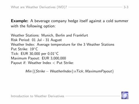
Example: A beverage company hedge itself against a cold summerwith the following option:
Weather Stations: Munich, Berlin and FrankfurtRisk Period: 01 Jul - 31 AugustWeather Index: Average temperature for the 3 Weather StationsPut Strike: 19◦CTick: EUR 30,000 per 0.01◦CMaximum Payout: EUR 3,000,000Payout if: Weather Index < Put Strike:
Min {(Strike −WeatherIndex) xTick;MaximumPayout}
Introduction to Weather Derivatives

What are Weather Derivatives (WD)? 3-4
Weather indices: temperature
Heating degree day (HDD): over a period [τ1, τ2]∫ τ2
τ1
max(T0 − Tu, 0)du (1)
Cooling degree day (CDD): over a period [τ1, τ2]∫ τ2
τ1
max(Tu − T0, 0)du (2)
T0 is some baseline temperature (typically 18◦C or 65◦F), Tu isthe average temperature on day u.
Introduction to Weather Derivatives
What are Weather Derivatives (WD)? 3-5
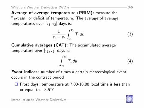
Average of average temperature (PRIM): measure the”excess” or deficit of temperature. The average of averagetemperatures over [τ1, τ2] days is:
1
τ1 − τ2
∫ τ2
τ1
Tudu (3)
Cumulative averages (CAT): The accumulated averagetemperature over [τ1, τ2] days is:∫ τ2
τ1
Tudu (4)
Event indices: number of times a certain meteorological eventoccurs in the contract period
� Frost days: temperature at 7:00-10.00 local time is less thanor equal to −3.5◦C
Introduction to Weather Derivatives
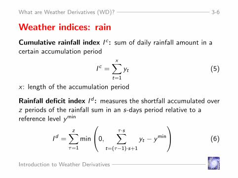
What are Weather Derivatives (WD)? 3-6
Weather indices: rain
Cumulative rainfall index I c : sum of daily rainfall amount in acertain accumulation period
I c =x∑
t=1
yt (5)
x : length of the accumulation period
Rainfall deficit index I d : measures the shortfall accumulated overz periods of the rainfall sum in an s-days period relative to areference level ymin
I d =z∑
τ=1
min
0,τ ·s∑
t=(τ−1)·s+1
yt − ymin
(6)
Introduction to Weather Derivatives
Valuation of WD 4-7
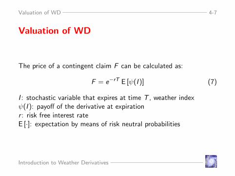
Valuation of WD
The price of a contingent claim F can be calculated as:
F = e−rT E [ψ(I )] (7)
I : stochastic variable that expires at time T , weather indexψ(I ): payoff of the derivative at expirationr : risk free interest rateE [·]: expectation by means of risk neutral probabilities
Introduction to Weather Derivatives
Valuation of WD 4-8
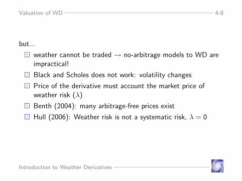
but...
� weather cannot be traded → no-arbitrage models to WD areimpractical!
� Black and Scholes does not work: volatility changes
� Price of the derivative must account the market price ofweather risk (λ)
� Benth (2004): many arbitrage-free prices exist
� Hull (2006): Weather risk is not a systematic risk, λ = 0
Introduction to Weather Derivatives
Valuation of WD 4-9
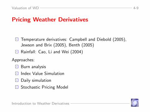
Pricing Weather Derivatives
� Temperature derivatives: Campbell and Diebold (2005),Jewson and Brix (2005), Benth (2005)
� Rainfall: Cao, Li and Wei (2004)
Approaches:
� Burn analysis
� Index Value Simulation
� Daily simulation
� Stochastic Pricing Model
Introduction to Weather Derivatives
Valuation of WD 4-10
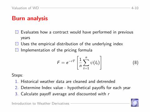
Burn analysis
� Evaluates how a contract would have performed in previousyears
� Uses the empirical distribution of the underlying index
� Implementation of the pricing formula
F = e−rT
[1
n
n∑t=1
ψ(It)
](8)
Steps:
1. Historical weather data are cleaned and detrended
2. Determine Index value - hypothetical payoffs for each year
3. Calculate payoff average and discounted with r
Introduction to Weather Derivatives

Valuation of WD 4-11
Call option price:
F = e−rT
[1
n
n∑t=1
{It − K , 0}+
]
Put option price:
F = e−rT
[1
n
n∑t=1
{K − It , 0}+
]
r : risk free interest rateK : strikeIt : accumulated weather index for t-th yearn: number of years
Introduction to Weather Derivatives

Valuation of WD 4-12
Index Value simulation
� Utilizes a statistical model for the weather index or thederivative payoff
� Supported by goodness of fit tests
Steps:
1. Given an appropriate distribution, the values of the index arerandomly drawn and the payoffs are determined
2. Calculate payoff average and discounted with r
Introduction to Weather Derivatives
Valuation of WD 4-13
Daily simulation
� Describes the dynamics of the weather variable over time
� Yield smaller confidence intervals than Burn and indexsimulation: smaller for rainfall than for temperature
Steps:
1. Derive the weather index from the simulated sample pathI summing up daily precipitation/daily average temperature
2. Determined pay offs
3. Calculate payoff average and discounted with r
Introduction to Weather Derivatives

Valuation of WD 4-14
Stochastic Model for temperature
Define the Ornstein-Uhlenbleck process Xt ∈ Rp:
dXt = Atdt +pt σtdBt
ekp: k’th unit vector in Rp
σt : temperature volatilityA: p × p-matrixBt : Wiener Process
A =
(0 1
−αp ... −α1
)Solution of Xt :
Xs = exp (A(s−t))x +
∫ s
texp (A(s − u))epσudBu
Introduction to Weather Derivatives
Valuation of WD 4-15
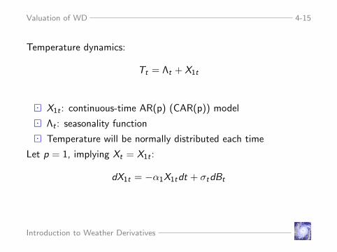
Temperature dynamics:
Tt = Λt + X1t
� X1t : continuous-time AR(p) (CAR(p)) model
� Λt : seasonality function
� Temperature will be normally distributed each time
Let p = 1, implying Xt = X1t :
dX1t = −α1X1tdt + σtdBt
Introduction to Weather Derivatives

Valuation of WD 4-16
Berlin temperature data
Daily average temperatures: 1950/1/1-2006/7/24
� Station: BERLIN-TEMP.(FLUGWEWA)� 29 February removed� 20645 recordings
Introduction to Weather Derivatives

Valuation of WD 4-17
Seasonal function
Suppose seasonal function with trend:
Λt = a0 + a1t + a2sin
(2π(t)
365− a3
)Estimates: a0 = 86.0543, a1 = 0.0008, a2 = 98.0582, a3 = 174.058Squared 2-norm of the residual at x:
minx{1
2‖Λt − Tt‖2
2} =1
2
m∑t=1
(Λt − Tt)2 = 3.02 + e07
Introduction to Weather Derivatives
Valuation of WD 4-18
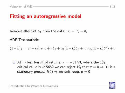
Fitting an autoregressive model
Remove effect of Λt from the data: Yi = Ti − Λi
ADF-Test statistic:
(1−L)y = c1 +c2trend+ τLy +α1(1−L)Ly + . . . αp(1−L)Lpy +u
� ADF-Test Result of returns: τ = −51.53, where the 1%critical value is -2.5659 we can reject H0 that τ = 0 ⇒ Yi is astationary process I (0) ⇒ no unit roots d = 0
Introduction to Weather Derivatives
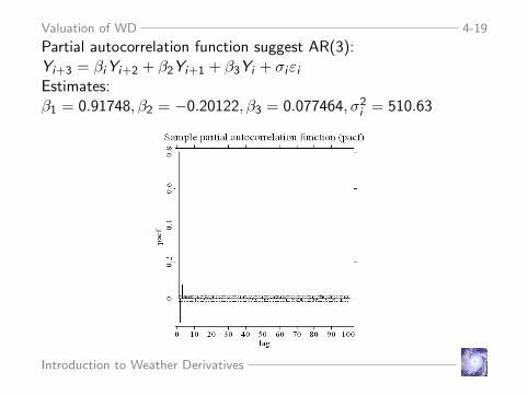
Valuation of WD 4-19
Partial autocorrelation function suggest AR(3):Yi+3 = βiYi+2 + β2Yi+1 + β3Yi + σiεiEstimates:β1 = 0.91748, β2 = −0.20122, β3 = 0.077464, σ2
i = 510.63
Introduction to Weather Derivatives
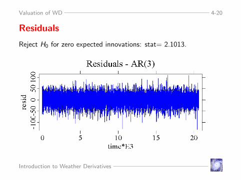
Valuation of WD 4-20
Residuals
Reject H0 for zero expected innovations: stat= 2.1013.
Introduction to Weather Derivatives

Valuation of WD 4-21
Seasonal volatility
Close to zero ACF for residuals of AR(3) and highly seasonal ACFfor squared residuals of AR(3)
Figure 1: ACFIntroduction to Weather Derivatives

Valuation of WD 4-22
Figure 2: PACF
Introduction to Weather Derivatives
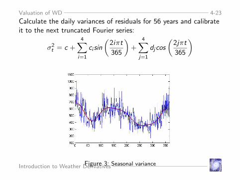
Valuation of WD 4-23
Calculate the daily variances of residuals for 56 years and calibrateit to the next truncated Fourier series:
σ2t = c +
4∑i=1
ci sin
(2iπt
365
)+
4∑j=1
djcos
(2jπt
365
)
Figure 3: Seasonal varianceIntroduction to Weather Derivatives

Valuation of WD 4-24
Dividing out the seasonal volatility from the regression residuals:
� ACF for residuals unchanged, residuals become normallydistributed
� ACF for squared residuals non-seasonal
Figure 4: Residual/seasonal variance
Introduction to Weather Derivatives

Valuation of WD 4-25
Temperature futures
HDD-futures price FHDD(t,τ1,τ2) at time t ≤ τ1:
FHDD(t,τ1,τ2) = EQ
[∫ τ2
τ1
max(18◦C − Tu, 0)du|Ft
]No trade in settlement periodConstant interest rate rQ is a risk neutral probability
� Not unique since market is incomplete
� Temperature is not tradable
Analogously: CDD and CAT future prices
Introduction to Weather Derivatives

Valuation of WD 4-26
Risk neutral probabilities
Defined by the Girsanov transformation of Bt : dBθt = dBt − θtdt
θt : time-dependent market price of risk.
Density of Qθ:
Z θt = exp
(∫ t
0θsdBs −
1
2
∫ t
0θ2s ds
)Dynamics Xt under Qθ:
dXt = (AXt + epσtθt)dt + epσtdBθt
with solution:
Xs = exp (A(s−t))x +
∫ s
texp (A(s−u))epσuθudu
+
∫ s
texp (A(s−u))epσudBθ
u (9)Introduction to Weather Derivatives
Valuation of WD 4-27
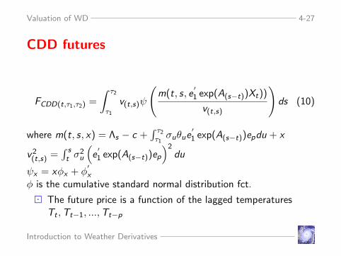
CDD futures
FCDD(t,τ1,τ2) =
∫ τ2
τ1
v(t,s)ψ
(m(t, s, e
′1 exp(A(s−t))Xt))
v(t,s)
)ds (10)
where m(t, s, x) = Λs − c +∫ τ2
τ1σuθue
′1 exp(A(s−t))epdu + x
v2(t,s) =
∫ st σ
2u
(e
′1 exp(A(s−t))ep
)2du
ψx = xφx + φ′x
φ is the cumulative standard normal distribution fct.
� The future price is a function of the lagged temperaturesTt ,Tt−1, ...,Tt−p
Introduction to Weather Derivatives
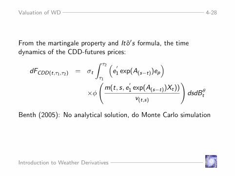
Valuation of WD 4-28
From the martingale property and Ito ′s formula, the timedynamics of the CDD-futures prices:
dFCDD(t,τ1,τ2) = σt
∫ τ2
τ1
(e
′1 exp(A(s−t))ep
)×φ
(m(t, s, e
′1 exp(A(s−t))Xt))
v(t,s)
)dsdBθ
t
Benth (2005): No analytical solution, do Monte Carlo simulation
Introduction to Weather Derivatives
Valuation of WD 4-29
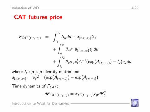
CAT futures price
FCAT (t,τ1,τ2) =
∫ τ2
τ1
Λudu + a(t,τ1,τ2)Xt
+
∫ τ2
τ1
θuσua(t,τ1,τ2)epdu
+
∫ τ2
τ1
θuσue′1A
−1(exp(A(τ2−u))− Ip)epdu
where Ip : p × p identity matrix anda(t,τ1,τ2) = e
′1A
−1(exp(A(τ2−u))− exp(A(τ1−t))
Time dynamics of FCAT :
dFCAT (t,τ1,τ2) = σta(t,τ1,τ2)epdBθt
Introduction to Weather Derivatives
Valuation of WD 4-30
Data adjustments
Station changes
� Instrumentation
� Location
Trends: to capture weather surprise
� Global Climate Cycles
� Urban heat
Forecasting
Introduction to Weather Derivatives

Research 5-31
Questions for Research
� Memory in AR(3): volatility with monthly/weeklymeasurement period
� Role of the strike value
� Longterm (interannual) variability of parameters - capturevolatility due to climate changes
� Relationship between weather variables and production
� Formula for options on CAT/CDD/HDD futures
� WD related to catastrophes
Introduction to Weather Derivatives

Conclusion 6-1
Conclusion
� CAR(p) model for the temperature dynamicsI Autoregressive process with seasonal mean and seasonal
volatility
� Analytical future prices for the traded contract on CMEI HDD/CDD/CAT/ futures with delivery over months or seasons
Introduction to Weather Derivatives

Conclusion 6-2
Reference
F.E. BenthOption Theory with Stochastic Analysis: An Introduction toMathematical Finance(Berlin: Springer), 2004.
Benth and S. BenthStochastic Modelling of temperature variations with a viewtowards weather derivatives(Appl.Math. Finance), 2005.
K. BurneckiWeather derivatives(Warsaw), 2004.
Introduction to Weather Derivatives

Conclusion 6-3
S. Cambell, F. DieboldWeather Forecasting for weather derivativesJ.American Stat. Assoc. , 2006.
J.C. HullOption, Futures and other Derivatives(6th ed. New Jersey: Prentice Hall International), 2006.
M. OdeningAnalysis of Rainfall Derivatives using Daily precipitationmodels: opportunities and pitfalls
Introduction to Weather Derivatives