Weather Derivatives in Russia: Insuring Farmers Against ... · This project proposes the use of...

i

Weather Derivatives in Russia: Insuring Farmers Against Temperature Fluctuations

Figure 1. Derivative Effect for Farmers

Submitted by:

Eric Carkin Stanislav Chekirov

Anastasia Echimova Caroline Johnston

Congshan Li Vladislav Secrieru Alyona Strelnikova

Marshall Trier Vladislav Trubnikov

Submitted to:

Professor Svetlana Nikitina Worcester Polytechnic Institute

Alexander Ilyinsky

Financial University under the Government of the Russian Federation

Date: 11 October 2017

ii

Abstract This project proposes the use of weather derivatives, a type of financial instrument

with a payout based on weather conditions, as a method for Russian farmers to hedge against daily temperature fluctuations. We created a weather derivative simulation tool in Microsoft Excel that calculates the effect of temperature on crop yield and then analyzes how the return of weather derivatives can potentially compensate for crop loss. Based on this tool, we developed a series of recommendations to help implement this system of protection with real users.

iii

Executive Summary

iv

Acknowledgements Our team would like to thank the following individuals for their contributions to the completion of our project:

● Worcester Polytechnic Institute and The Financial University Under the Government of the Russian Federation for providing us with the means and opportunity to complete this project.

● Alexander Ilyinsky, Dean of the International Finance Department at the Finanical University, for his guidance and for planning the foundations of the project as our sponsor.

● Tatiana Goroshnikova, Deputy Dean of the International Finance Department at the Financial University, for her weekly advice and guidance.

● Svetlana Chugunova for organizing our stay and accommodations while in Russia. ● Oleg Pavlov, Stephan Sturm, Gbetonmasse Somasse, Michael Radzicki, Michael

Johnson, and Anton Losev, for sharing the knowledge of their respective fields during our interviews and team meetings.

● Svetlana Nikitina for coordinating with The Financial University Under the Government of the Russian Federation to make this project possible. We also would like to thank her for her continual guidance throughout the duration of the project as our advisor.

v

TABLE OF CONTENTS TITLE PAGE……………………………………………………………………………………....…...…….……………….....i ABSTRACT……………………………………………………………………………………………………………………...ii EXECUTIVE SUMMARY……………………………………………...…….……...…….……...…….……...….………. iii ACKNOWLEDGEMENTS…...…….……...…….……...…….……...…….……...…….……...…….……...…….…….. iv TABLE OF CONTENTS………………………………………………………...……………….…...…….……...……..… v TABLE OF FIGURES………....…………………………………………………….…………..…...…….……...…….….. vi TABLE OF TABLES………………………………………………………………………………………………………...vii 1. UTILIZING WEATHER DERIVATIVES IN RUSSIA……………………………….…...…….………………..1 2. USING WEATHER DERIVATIVES TO INSURE RUSSIAN AGRICULTURE……..…...………..…….. 2

2.1. Weather Risks and Mitigation Strategies.................................................................. …………2 2.2. Weather Derivatives………………………………………….…………...…...…….…... ………………2 2.3. Non-Russian Weather Derivatives Systems………………………. …………………………….3 2.4. Agriculture in the Moscow, Krasnodar, and Omsk Regions….....……...……...…….. …..4 2.5. The Shortcomings of the Russian Government Subsidies System………….…………..5 2.6 Conclusion………………………………………………………………………………………………...…....6

3. METHODOLOGY: DEVELOPING A WEATHER DERIVATIVES SYSTEM.…………...……...…….. ...7 3.1. Determining Relationship Between Temperature and Crop Yield………..……...........8 3.2. Pricing Weather Derivatives ……...……...……...……...……...……...……...……...……......….....8 3.3. Creating Simulation Tool..……...……...…….……...…………………………………………………. 8 3.4 Conclusion…………………………………………....……………………………………………………… .9

4. Results and Discussion ……...……...……...……...……...……...……...……...……...……...……...…………...10 4.1. Determining Relationship Between Temperature and Crop Yield…………………...10 4.2. Pricing Weather Derivatives………………………………………………………………………....12 4.3. Creating Simulation Tool………………………………………………………………………………12 4.4. Testing Simulation Tool………………………………………………………………………. ……...13 4.5. Advantages of the Simulation Tool……………………………………………………...………... 15

5. Conclusions and Recommendations……...……...……...……...……...……...……...……...…….……… …16 5.1. Testing with Real Users……………………………………………………………………………. …16 5.2. Promoting the Tool……………………………………………………………………………………....16 5.3. Testing the Effect of Precipitation and Constructing Precipitation-based Derivatives…….. ……………………………………………………………………………………...........16 Derivatives………………………………………………………...............................................……14 5.4. Optimizing Pricing Parameters……………………………………………………………….……. 17 5.5. Evaluating Other Pricing Methods………………………………………………………………. ..17 5.6. Trading Weather Derivatives………………………………………………………………………. .18 5.7. Conclusion…………………………………………………………………………………………………...18

REFERENCES……………………………………………………………………………………………………………….. 19 APPENDICES……………………………………………………………………………...………………………………....22

A. Relevant Equations………..…………………………....………………………………………………...22 B. Crop Planting and Harvest Dates…………………………………………………………………. ..24 C. Record of Project Development………………………………………………………. ………….…25 D. Simulation Tool VBA Code…………………………………………………………………………….27

vi

TABLE OF FIGURES

Figure 1: Derivative Effect for Farmers……………………………. ……………….………………………………i Figure 2: Regions of focus: Left-Krasnodar, Center-Moscow, Right-Omsk………………………..…1

Figure 3: Adapted from Growth and Development Guide for Spring Wheat………….……… ……3 Figure 4. Russian grain production 1992-2016………………………………………………………..………. 5 Figure 5: Methodology strategy layout……………………………………………………………………………..7 Figure 6: Collecting data from the Bloomberg Terminal…………………………………………………… 9 Figure 7: Krasnodar spring wheat GDD/yield before data pre-processing………………… …….10 Figure 8: Trend between land acreage and crop yield for Krasnodar winter wheat ...........… 11 Figure 9: Krasnodar spring wheat and Moscow corn regression results…………………… ...…..12 Figure 10: Tool interface…………………………………………………………………………………………… ….13 Figure 11: Accuracy of Predicted Yield Values…………………………………………………………. …….14 Figure 12: Accuracy of Predicted GDD Values………………………………………………………….. …….14 Figure 13: Profits with yield and weather derivative use…………………………………………….…..14 Figure 14: Team photo…………………………………………………………………………………………………..25 Figure 15: Vladislav T. and Caroline presenting on the pricing of weather derivatives…… ..25 Figure 16: Anastasia and Eric presenting on educating farmers and the simulation tool… ..26 Figure 17: Taking a break from the project to enjoy Stanislav’s magic tricks…………………… 26

vii

TABLE OF TABLES Table 1: Yield Per Area vs Cumulative GDD Regression R2 Values……………… ……………………12 Table 2: Derivative Parameters…………………………………………………………………….. ……………....23

Table 3: Potato, Corn, and Wheat Planting/Harvest Dates……...... …………………………………….24

Table 4: Moscow, Krasnodar, and Omsk frost dates. ……………………………………………………….24

1

1. Utilizing Weather Derivatives in Russia In 1998 it was estimated that 20% of the world economy is vulnerable to weather conditions (Barrieu & Scaillet, 2010). Weather is one of the most uncontrollable and influential variables within the agriculture sector, becoming increasingly unpredictable as climate change continues to affect global weather patterns. In some cases, extreme weather can cause up to a 40% deficit in crop yields in Russia, potentially devastating a farmer’s economic income (Pavlova, Varcheva, Bokusheva, & Calanca, 2014). However, by utilizing various types of insurance, those in the agricultural sector are able to survive and continue to develop by mitigating their exposure to this financial risk.

Russia’s ambitions to become agriculturally self-sufficient and the country’s ban on imported crops have caused its agricultural sector to grow substantially in recent years (Liefert, Serova and Liefert, 2015). In order to foster this growth and continue to develop this sector, farmers are in need of insurance policies to protect themselves from risks that are beyond their control, such as weather. Weather derivatives, a type of financial option, can be used to protect farmers from daily fluctuations in temperature and precipitation that catastrophic insurance plans do not shield them from (Chung, 2011). These events have a modest effect over a single day but cumulatively they can have severe effects on a farmer’s yield by the end of the growing season. Though weather derivatives have been used to hedge against risks in other countries, Russia has yet to explore this tool and popularize it among its farmers (Esper Group, 2010).

The goal of this project is to create a proof-of-concept weather derivatives pricing system. This system will explore the feasibility of insuring farmers within Russia using such financial instruments. Farmers will be able to hedge against weather-related risks by trading weather derivative options and to remain financially stable even in times of fluctuating weather conditions. In order to accomplish this goal, we had to meet the following objectives:

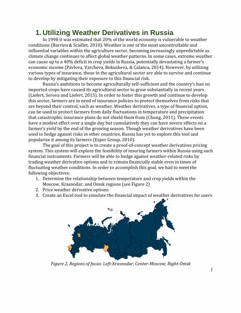
1. Determine the relationship between temperature and crop yields within the Moscow, Krasnodar, and Omsk regions (see Figure 2)

2. Price weather derivative options 3. Create an Excel tool to simulate the financial impact of weather derivatives for users

Figure 2. Regions of focus: Left-Krasnodar, Center-Moscow, Right-Omsk

2

2. Using Weather Derivatives to Insure Russian Agriculture

In order to implement a weather derivatives system within Russia, one must understand the relationship between weather and agriculture and the current measures in place to protect farmers against weather risks. In this chapter we will explain the concept of a weather derivative as a means to hedge against these risks. Then we will discuss Russia’s current agricultural economy and strategies to protect those working in agriculture from losses due to weather events. 2.1. Weather Risks and Mitigation Strategies

Weather conditions directly affect an estimated 20% of the world economy. The associated economic risks tied to weather can be divided into two major groups: high frequency-low risk events and low frequency-high risk events. Low frequency-high risk events, such as tornadoes and hurricanes, have an extreme, immediate impact, costing millions of dollars in damages. High frequency-low risk events are everyday weather phenomena, such as rain and temperature change. These events cause little impact over a single day but cumulatively can cause substantial, negative effects. The agricultural sector is especially sensitive to this type of risk, causing weather to have a considerable effect on the economy (Barrieu & Scaillet, 2010). Governments across the globe have set up various forms of insurance, such as government subsidies or weather derivatives, to protect those working within the agricultural sector. The use of government subsidies in times of poor harvest however is not always ideal or even feasible for less developed countries that cannot generate enough revenue from taxation. Additionally, subsidy compensation is based on a farmer’s exact loss, requiring insurers to determine farmer’s yields in order to calculate what compensation is due. This increases costs to the insurer and in turn raises the cost of premiums for those who are insured (Chung, 2011).

2.2. Weather Derivatives

Weather derivatives offer advantages to both small-scale farmers and corporate agricultural businesses. These derivatives are a type of option with an index-based payout, modeled after predicted future weather conditions over a certain period of time. The major difference between a weather derivative and subsidy is that the payout for a derivative is based on the specific weather conditions that cause farming loss, while a payout for a subsidy is based on the actual loss itself. Thus, weather derivatives are able to cover the high frequency-low risk events described above- without the need for insurers to determine farmer’s exact yields, keeping premium costs lower (Chung, 2011).

There are still many adversities to overcome in order to utilize weather derivatives effectively (Chung, 2011). For example, as discussed above, a substantial amount of meteorological data is required to price the derivative with any degree of accuracy.

3

Collecting this data can take an enormous amount of time and resources but is absolutely vital for constructing an accurate index for making weather predictions.

Around 75% of all weather derivative transactions are based upon temperature predictions while 10% are based upon rainfall (Barrieu & Scaillet, 2010). Temperature- indexed weather derivatives revolve around the concept of Growing Degree Day (GDD), which measures heat accumulation to predict favorable plant development rates and stages of growth (see Figure 3, Appendix A). The metric below computes the difference between realized temperatures to a baseline temperature, which varies depending on the crop species (e.g. baseline temperature is 7.2 °C for potatoes, 4.4 degrees °C for wheat, etc.).

Figure 3. Adapted from Growth and Development Guide for Spring Wheat (Simmons,

Oelke and Anderson, 1985)

2.3. Non-Russian Weather Derivatives Systems While weather derivatives are still a fledgling concept, being first traded on the Chicago Mercantile Exchange (CME) in 1999, their use is slowly becoming more commonplace within global markets outside of Russia (Barrieu & Scaillet, 2010). The Canadian agricultural insurance market recently introduced weather derivatives to insure against abnormal season temperatures or precipitation levels. After interviewing 397 farmers from Saskatchewan over a period of three years, investigators showed that 307 of these farmers used only traditional agricultural insurance, 37 only used weather derivatives, and 37 used both types of insurance. The study concluded that this wide disparity in weather derivative use is mainly attributed to farmers’ lack of “awareness and understanding” of the tool (Van Camp, 2015, para. 5). About half of the participants who

4

did not invest in weather derivatives were not aware that such a tool was available to them. About one-third of these farmers felt they did not have enough knowledge and skill to utilize the derivative (Van Camp, 2015). In 2003, a Mumbai insurance company implemented weather derivatives for small groundnut and castor farmers in four villages within the Andhra-Pradesh state. The program encouraged farmers to attend educational workshops about the product to properly inform farmers of what this insurance is and its benefits, increasing the derivative’s approachability. In 2005 after more improvements to the program, “more than 250000 [sic] farmers bought weather insurance” (Barrieu & Scaillet, 2010, 7). This pilot weather derivatives project in India was deemed a major success and inspired many more weather-based insurance schemes across India such as the Weather-based Crop Insurance Scheme (WBCIS) (Ministry of Finance of India, 2017).

One of the main distinctions between the Indian and the Canadian weather derivatives program is the presence of an educational program for the users. Equipped with the knowledge of how these weather derivatives could financially support them, farmers in India widely supported the weather derivatives system. However, those in Canada struggled to see the potential benefits of these tools or were completely unaware of them. Thus, in order to build a successful and accessible weather derivative system, it is vital to educate the users.

2.4. Agriculture in the Moscow, Krasnodar, and Omsk Regions The Russian agriculture sector employs 7.7 million people, or 12% of the total workforce (British Potato Council, 2006). Concurrently, most of Russia's land mass is considered to be in "risky farming zones," where the harvest capacity, or these farmers’ economic livelihoods depends largely on weather conditions. This is exacerbated by global climate change, which makes weather conditions increasingly more unpredictable. Because of the country’s geographic span, the overall climate of Russia varies significantly from north to south and east to west, allowing different crops to thrive in different areas and temperatures (Country Studies, 1996). These differences in temperature not only affect the rate at which these crops grow, but also the dates on which they are planted and harvested, creating a unique set of growing conditions for each crop in each region.

Wheat, corn, and potatoes are three of the most widely-grown crops within Russia (Basic Element, 2013). Grains occupy more than 50% of the available cropland, primarily in the form of wheat (Country Studies, 1996). The overall land productivity is recently on the rise due to a decrease in the price of the ruble and recent favorable growing conditions (see Figure 4) (Medetsky, 2016). These large yields have brought in a substantial income for farmers, but again, only on the condition of favorable weather conditions. Thus, the agricultural sector is currently a lucrative investment area but not without potential risks.

The Moscow, Krasnodar, and Omsk regions provide a representative range of Russian climatic and agricultural conditions. The Moscow region is located in the western part of the country. Because of its large population, its local agriculture has a high profile. Krasnodar is the economic center of southern Russia, and 42.8% of its main industries is

5

agriculture-based (Oleynik ,2013). Because of Krasnodar’s geolocation by the Black Sea, the region has a longer growing season and more ideal weather conditions for plant growth (State's executives of the Krasnodar Region, n.d.). Conversely, the growing conditions in Omsk are not as favorable. Situated on the West Siberian Plain, the annual average temperature in Omsk is around 1.4℃ (Climatemp, n.d.). Wheat, corn, and potatoes are grown in all three areas, but each is subject to the region’s unique weather conditions.

Figure 4. Russian grain production 1992-2016 (Medetsky, 2016)

2.5. The Shortcomings of the Russian Government Subsidies System

Government subsidies are currently used to help farmers in Russia hedge against weather risks (Buckley, 2017). State-issued subsidies have created significant growth within the agricultural sector, but not without complications. Some farmers cannot afford premiums, cannot meet land acreage requirements, or do not have the necessary accounting paperwork to qualify for these payments. In the 2012 drought, state compensation was only given to farmers “located in emergency districts… in a manner that was not at all transparent [to the farmers],” while those located in “non-emergency” zones suffered terrible losses as well (Ukhova, 2013, 12). Those who received payment received dismally insufficient amounts of compensation in comparison to their actual loss. The amount of red tape and underperformance from subsidies has resulted in a general lack of faith in the system (Ukhova, 2013). To work towards restoring this faith and efficiency, farmers must be able to easily access their method of compensation and understand why they are receiving it. Even with these improvements, subsidies only protect against high-impact events such as a drought. There is still a clear lack of protection against small but continual risk such as temperature fluctuations (Esper Group, 2010).

6

2.6. Conclusion Weather derivatives can be used to insure farmers against daily fluctuations in temperature, which can have a substantial impact on their yields, and thus their wallets. Most of the farmland within Russia is highly sensitive to weather conditions. Though government subsidies have been used in the past to assist farmers in protecting themselves against weather risks, farmers no longer trust this specific system. Weather derivatives, however, use objective weather data and minimal bureaucratic procedures to help farmers compensate for their losses incurred by unfavorable weather conditions. As shown in the Indian and Canadian contexts, for the concept of a weather derivative to work it has to be familiar to farmers, and it is vital that they are educated about this tool’s use and benefits. This builds trust and extends the use of an effective weather derivatives system.

7

3. Methodology: Developing a Weather Derivatives System

The goal of this project is to create a proof-of-concept weather derivatives pricing system. This system will explore the feasibility of insuring farmers within Russia using such financial instruments. As can be seen in Figure 5, we created the following objectives to successfully reach this goal:

1. Determine the relationship between temperature and crop yield within the Moscow, Krasnodar, and Omsk regions

2. Price weather derivative options 3. Create an Excel tool to simulate the financial impact of weather derivatives

for users

Figure 5. Methodology strategy layout

8

3.1. Determining Relationship between Temperature and Crop Yield Because the pricing of weather derivatives depends upon GDDs that are crop-specific, we selected 3 regions and 3 specific crop types for the construction of derivatives. We identified corn, potatoes, and wheat (spring and winter) as some of the most common crops in Russia and the Moscow, Krasnodar, and Omsk regions as areas representing a spread of weather conditions. We gathered each crop’s baseline temperature for its GDD calculation, its planting dates, and its harvest dates. Using these dates and temperatures, we were able to accurately gauge the temperatures these crops experience within a growing season.

We calculated the mean cumulative GDD experienced by each crop within Moscow, Krasnodar, and Omsk regions from the years 1996 to 2015 with data from the meteo.ru (RIHMI-WDC) weather database and collected regional crop yield statistics from Knoema, another online database (see References). Using Microsoft Excel, we developed a database of these temperatures and implemented an ordinary least squares regression technique to quantify the relationship between cumulative GDD over the growing period and crop yield. 3.2. Pricing Weather Derivatives

In order to price the derivatives, we surveyed various pricing methods. After reviewing literature by Sun and van Kooten (2015); Groll, López-Cabrera, and Meyer-Brandis (2016); Taylor and Buizza (2006); Chung (2011); Alaton, Djehiche, and Stillberger (2002); Barrieu and Scaillet (2010); and Consedine (2000), we chose the historical burn analysis method, which takes the average historical GDD as the expected GDD for future years (see Appendix A). This technique was chosen because of its ability to accurately model these future GDD values, the accessibility of the data needed for this method, and the ability to conduct the necessary mathematical processes in a familiar format such as an Excel spreadsheet. 3.3. Creating Simulation Tool

To visually represent the results of this project and demonstrate the potential impact of this weather derivatives system, we created a weather derivative simulation tool in Visual Basic for Excel. This tool calculates the potential losses a farmer faces by interfacing with the GDD/yield relationship model. The farmer inputs his or her farm size, crop type, and location. His or her projected yield for the upcoming year is then calculated by utilizing the appropriate GDD/yield model, the projected GDD based on his or her region, and the size of his or her farm. This yield is then multiplied by the estimated worth of his or her crop, data gathered from Bloomberg, converting his or her potential profit to a monetary value (see Figure 6).

Based on the GDD/yield model, the tool also estimates potential economic loss if the weather varies from the expected GDD. A derivative is then constructed using the chosen tick size. The derivative’s payoff can be compared to a farmer's potential loss, showing its potential effectiveness as a form of insurance.

9

The tool draws upon values from the database mentioned in Section 3.1. Because all of the data inputs (excluding those provided by the user) are contained within Excel spreadsheets, the tool can be easily updated to include more recent information or different areas and crops, expanding it to become a more encompassing and accurate tool.

3.4. Conclusion

The cumulative application of our methods is showcased in the simulation tool. The tool is capable of evaluating the GDD/yield relationship for each region and crop, the predicted GDD values for future years, and the potential profit or loss with weather derivative use for a specific user. This allows the user to directly visualize the effect of a weather derivative and its potential as an insurance measure. Additionally, the tool is easily modifiable, allowing it to remain relevant and open for modification while further developments take place in this research field. By using this tool, those who are interested in developing derivative-based insurance can also test their own research methods and display these techniques to their target users.

Figure 6. Collecting data from the Bloomberg Terminal

10

4. Results and Discussion After initial poor results in our regression analysis for cumulative GDD and crop

yield, we found there were large flaws in the methods in which we were processing and interpreting our collected data. We then developed a strategy to correct these flaws to pre-process our data to eliminate trends that were contaminating our results. This lead to more accurate results. We produced a clearer relationship between the two variables. When pricing the derivative, the historical burn analysis generated high quality GDD predictions and generally low premiums for the farmers. Both the regression and the pricing calculations were implemented in our Excel simulation tool that is both flexible for those who wish to build upon it and approachable for farmers who wish to use it.

4.1. Determining Relationship between Temperature and Crop Yield

The regression between temperature and crop yield initially yielded fairly weak results and no clear or logical relationship has been obtained at that point (see Figure 7). After discussing the quality of our data, we isolated the causes of this weak regression result to two factors:

1.) Qualitative growing season data 2.) Skewed yield data

Figure 7. Krasnodar spring wheat GDD/yield before data pre-processing (1996-2015)

When collecting harvest and planting dates, we found that the data was extremely

qualitative, described as “early May”, “mid-September”, etc. This is perfectly reasonable for a farmer who plants when the soil is deemed ready, but not sufficient for quantitative analysis. In order to accurately model these decisions, we further researched the favorable planting conditions for our four crops. Then, based on this information, we created an algorithm to search through the temperature database and select a planting day that meets these conditions.

Each crop has its respective GDD criteria to meet to reach its planting date (see Appendix B). However, GDD is not the only factor used. The typical growing season for our

11

chosen crops covers a period of three months. Thus, our algorithm only selects a planting date that satisfies the GDD requirements within this time range. If this criteria was not met during this time period, the end of the time interval was selected as the planting date. This method of selecting planting dates creates a more accurate picture of actual GDD, giving us stronger models to predict crop growth. Harvest dates, on the other hand, remain relatively stable from year to year and do not require such attention.

We then realized that our collected yield data had varying amounts of total acreage per year contributing to this yield. An increased total acreage was resulting in an increased total yield for that year, i.e. causing a linear trend within the data (see Figure 8). Thus, to isolate the effects of GDDs on crop yield, we converted the raw yield data into yield per recorded acreage. The regression analysis then produced relatively strong results (see Figure 9 and Table 1). Thus, this relationship can be used to approximate how a predicted change in cumulative GDD in each region will affect the yield results for each crop, clearly demonstrating to the farmers their potential loss in yield. This is the first step in showcasing to them how the purchase of weather derivatives can compensate for this projected loss.

Figure 8. Trend between land acreage and crop yield for Krasnodar winter wheat (1996-

2015)

12

Table 1. Yield Per Area vs Cumulative GDD Regression R2 Values

Crop Moscow Krasnodar Omsk

Corn 0.276 0.201 0.137

Potato 0.026 0.247 0.195

Spring Wheat 0.211 0.428 0.26

Winter Wheat 0.083 0.259 0.057

Figure 9. Krasnodar spring wheat and Moscow corn regression results (1996-2015)

4.2. Pricing Weather Derivatives

Following the formulas for pricing the weather derivatives, the farmer profits whenever the GDD hits one of two appropriate points (see Appendix A). However, it was not entirely clear how to adjust these pricing parameters so that farmers with a larger amount of farmland and a greater economic loss from poor weather conditions would be able to buy a weather derivative in order to collect a larger payout. In other words, we could not establish a relationship between farm size and premium. Therefore, we decided to add tick size as a user input for our simulation tool.

4.3. Creating Simulation Tool

The final deliverable of our project is an easy-to-use tool that compiles all of our work and demonstrates the effectiveness of weather derivatives to farmers, while also serving as a stepping stone for a practical implementation of this project. The tool performs situation-specific calculations based upon profile information provided by the user, e.g. crop type, location, farm size, and tick size (see Figure 10). Using this information as a basis

13

for our parameters, the tool draws from a large Excel database to calculate the GDD/yield relationships, predicted GDDs and yields, the potential profit/loss of the farmer, and the price of the weather derivative. The farmer is then able to see his or her potential loss under various circumstances.

The program offers a large amount of flexibility in terms of upkeep, update potential, and data management. Data can easily be added into the Excel database for further processing as time passes and more weather and yield data is collected. The tool itself can easily be used by those with basic familiarity with Microsoft Office Products. The program’s functionality demonstrates the potential effectiveness of utilizing weather derivatives for farming insurance and serves as a flexible and scalable tool that can generate further interest in the development of a weather derivatives program.

Figure 10. Tool interface

4.4. Testing Simulation Tool In order to determine the accuracy of the simulation tool and whether weather

derivatives are an effective hedging tool for farmers, we added testing code to the tool. This test code takes the last 5 years of the data base (the years 2011 through 2015), and treats them as future years. For each of these years, we predict the GDD, the crop yield, and produce a derivative option. The actual yield and GDD are then compared to what was predicted to determine accuracy, and the farmer's profit is compared to the derivative return to determine its effectiveness. As each past year is tested, its information is added

14

back into the database for the next test calculation. The results show that as more data is added to the model, it becomes more accurate (see Figure 11 & 12). It also shows that with adjustment of the tick size, weather derivatives can help considerably to cover farmer’s losses (see Figure 13).

Figure 11. Accuracy of Predicted Yield Values

Figure 12. Accuracy of Predicted GDD Values

Figure 13. Profits with yield and weather derivative use

15

4.5. Advantages of the Simulation Tool

This simulation tool is effective in allowing other individuals to quickly visualize the potential benefits of utilizing weather derivatives as insurance. A farmer, or someone acting as a farmer for academic research, can input information that reflects their current economic position, and then gauge how effectively weather derivatives can mitigate their economic risks. In terms of development, it allows researchers to determine the efficiency of weather derivatives and adjust parameters as necessary when working towards a market implementation. For users, the tool’s ability to easily convey the savings delivered by a derivative should generate popular interest in the product. The creation of this tool will hopefully spur the development of derivative-based insurance systems throughout Russia to further boost the agricultural sector development.

16

5. Conclusions and Recommendations

From our project work we have compiled a list of recommendations for the further development of this weather derivative tool. Ultimately, we recommend:

1. Testing the tool with real users 2. Promoting the tool amongst real users 3. Conducting laboratory experiments to determine the effect of precipitation

on yield and create precipitation-based derivatives 4. Optimizing pricing parameters 5. Evaluating and applying other pricing techniques 6. Trading the weather derivatives on a local exchange trading system (LETS)

5.1. Testing with Real Users In order to further confirm the effectiveness and reliability of this tool, it is imperative that actual farmers test it. These farmers would complete surveys and/or take part in focus groups to evaluate the ease of use of this tool and its accessibility. Additionally, these farmers can be used to judge the robustness of the constructed models. Users would record their actual crop loss versus their predicted loss and their actual compensation from the weather derivatives. The differences in the actual conditions and projected conditions would then be used to create more accurate models. Working with more relevant data and tracking the actual outcomes of these farmers’ experiences would ultimately help to create a more beneficial tool in the future. 5.2. Promoting the Tool Once the tool has been sufficiently tested, it is important that farmers are aware that this tool exists. As described above, many Canadian farmers did not even know that weather derivatives existed or did not how they could be used to help them (Van Camp, 2015). Thus, we recommend that our tool is promoted in a marketing campaign. This promotion would involve researching the methods of communication that are most valuable to farmers (e.g. publications in an agricultural magazine, workshops like those in the India system, word-of-mouth, etc.) and then promoting through these methods. The farmers will never be aware of how this tool can help them if they are never aware of the tool itself. 5.3. Testing the Effect of Precipitation and Constructing Precipitation-based Derivatives

One issue we encountered during the development of the GDD/yield model is that, even with the preprocessing of data, cumulative GDD is undoubtedly not the only factor that determines crop growth. As evident in Figure 9, some years experience a similar GDD but vastly different yields.

Precipitation also plays a key role in crop development. With global changes in climate and unstable precipitation patterns, it is especially important to factor in more than just temperature into our yield response model. Thus, we recommend conducting a future

17

laboratory experiment that analyzes the effect precipitation has on overall yield for these crops. This experiment would expose crops to the same cumulative GDD, but change the amount of water each plant receives and document each crop’s growth rates. A similar experiment should also be conducted that maintains constant water levels and varies the GDDs.

Comparing the results of each of these tests would reveal which factor is more critical for the growth of different crops. A similar precipitation/yield model could be constructed so that farmers can visualize how future rainfall predictions will affect their crops. Weather derivatives based on a cumulative rainfall index could also be priced if necessary. This will allow farmers to pick between a GDD or a precipitation derivative, depending on whichever is more unpredictable and/or influential in their region.

5.4. Optimizing Pricing Parameters

The goal of this weather derivatives system is to compensate farmers for their agricultural losses due to unfavorable weather conditions. The weather derivative makes a payment to the farmer under certain temperature conditions, but further research must be done to optimize the pricing parameters to ensure that farmers’ premiums are affordable to the farmer and that these payouts provide substantial compensations. For example, the strike values of the weather derivative are currently set at 0.2 standard deviations away from the mean cumulative GDD values. By setting the strike values at a larger standard deviation away, we could decrease the cost of the premium, but also decrease the likelihood of receiving payout from the derivative. Thus, a balance must be found between the initial premium cost and meaningful levels of compensation when the weather conditions are not favorable.

5.5. Evaluating Other Pricing Methods

Finding the best methods to price weather derivatives is an open research problem. As stated before, we selected the historical burn analysis and because the data needed for processing was accessible and the technique proved to be effective in previous research papers. The mathematical concepts presented were also easy to grasp and implement by our team in Excel within a limited timeframe.

Currently more accurate methods of pricing exist, even if they were not feasible for our team to calculate. For example, Taylor and Buizza (2006) use ensemble forecasting to create their weather prediction model with data provided by the European Centre for Medium-range Weather Forecasts (ECMWF), a source which we did not have access to. With higher-fidelity forecasting models, more accurate derivative pricing will ensue and more protection will be provided to the farmers. Because weather prediction continues to be uncertain, we recommend a more comprehensive comparison of weather derivative pricing that encompasses techniques outside of those presented here. This will either affirm the accuracy of our methods or provide even more accurate pricing methods.

18

5.6. Trading Weather Derivatives

Most weather derivatives are currently traded on the market using over-the-counter (OTC) transactions, meaning they are not traded on formal exchange systems like NASDAQ or Dow Jones but privately negotiated between two parties (Investopedia, n.d.). We did not pursue research into bringing the derivatives to a real-world market due to lack of time for the project. Eventually this weather derivatives system should be brought out of academia and into the real-world. We recommend further research into trading derivatives on an online local exchange trading system (LETS) so that contracts can be easily bought and sold all around the world. Additionally, all derivative transactions could take place utilizing Blockchain technology, eliminating the need for clearing houses as well as third-party security issues. This would also decrease costs to users and increase their profits (Iansiti & Lahkani, 2017). 5.7. Conclusion

With global climate change altering weather patterns, Russian farmers are in need of protection from everyday weather events that will negatively affect their crop yields. This type of protection is not currently offered through traditional methods of agricultural insurance or government subsidies and furthermore, Russian farmers have a lack of faith in these products. Through the use of weather derivatives, these farmers should be able to hedge these risks at an affordable premium price. To build a weather derivative simulation tool, our team constructed a model that demonstrates the relationship between cumulative GDD within a growing season and crop yield for corn, potatoes, and wheat in the Moscow, Krasnodar, and Omsk regions. We were then able to price weather derivatives, displaying these results and models on the Excel simulation tool. This tool is able to demonstrate how predicted GDDs will affect farmers’ yields and how they can protect themselves from potential economic loss and thus boost popular interest in a weather derivatives system in Russia.

https://hbr.org/search?term=marco+iansiti

19

References

Alaton, P., Djehiche B., & Stillberger D. (2002). On Modeling and Pricing Weather Derivatives. Retrieved from http://dx.doi.org/10.1080/13504860210132897

APK-Inform. (2004). Optimum Terms of Harvesting of Winter Wheat In The Central Region

of Ukraine. Retrieved from http://www.apk-inform.com/ru/news/17539

Basic Element (2013) The Future of Farming in Russia. «Базовый Элемент», Farmers Weekly. Retrieved from www.basel.ru/en/articles/farming_09_12_13/. Barrieu, P., & Scaillet, O. (2010). A primer on weather derivatives. In Uncertainty and

Environmental Decision Making: A Handbook of Research and Best Practice (pp. 155-175). Retrieved from http://1cellonelight.com/pdf/weatherCambridge.pdf

British Potato Council. (2006, August). Target market report for the export of GB seed potatoes. BPC Target Market Report Russia. Retrieved from https://potatoes.ahdb.org.uk/sites/default/files/publication_upload/BPC%20 OMIS%20Report%20Russia.pdf Buckley, N. (2017, April). Russian Agriculture Flourishes Amid Sanctions. Financial

Times. Retrieved from https://www.ft.com/content/422a8252-2443-11e7-8691-d5f7e0cd0a16

Cereals of Russia. Sowing of Spring Wheat. (n.d.). Retrieved from

http://www.activestudy.info/posev-yarovoj-pshenicy/

Climatemp (n.d.). Omsk Weather and Temperature. Retrieved from http://www.omsk.climatemps.com/

Chung, W. (2011). Evaluating weather derivatives and crop insurance for farm production risk management in southern Minnesota. Master’s thesis, University of Minnesota. Retrieved from https://conservancy.umn.edu/bitstream/handle/11299/119325/Chung_umn_0130E_12390.pdf?sequence=1&isAllowed=y

Consedine, G. (2000). Introduction to Weather Derivatives. CME Group. Retrieved from https://www.cmegroup.com/trading/weather/files/WEA_intro_to_weather_der.pdf Country Studies. (1996). Agriculture. Country Studies. Retrieved from http://countrystudies.us/russia/60.htm Esper Group. (2010). NO CLIMAT but weather. Esper Times. Retrieved from http://www.esper-group.com/files/4/Esper-Times-_30-eng.pdf Glenn, J. (2017). Euro vs. US Dollar. Investor Guide. Retrieved from http://www.investorguide.com/article/15564/euro-vs-us-dollar-d1412/ Groll, A., López-Cabrera, B., & Meyer-Brandis, T. (2016). A consistent two-factor model for pricing temperature derivatives. Energy Economics, 55, 112-126. Retrieved from http://www.sciencedirect.com/science/article/pii/S0140988316000104 Growing Guide. (2006). Potatoes. Retrieved from

http://www.gardening.cornell.edu/homegardening/scenec6be.html

http://dx.doi.org/10.1080/13504860210132897

http://www.apk-inform.com/ru/news/17539

http://www.basel.ru/en/articles/farming_09_12_13/

http://1cellonelight.com/pdf/weatherCambridge.pdf

https://potatoes.ahdb.org.uk/sites/default/files/publication_upload/BPC%20OMIS%20Report%20Russia.pdf

https://potatoes.ahdb.org.uk/sites/default/files/publication_upload/BPC%20OMIS%20Report%20Russia.pdf

https://www.ft.com/content/422a8252-2443-11e7-8691-d5f7e0cd0a16

https://www.ft.com/content/422a8252-2443-11e7-8691-d5f7e0cd0a16

http://www.activestudy.info/posev-yarovoj-pshenicy/

http://www.omsk.climatemps.com/

https://conservancy.umn.edu/bitstream/handle/11299/119325/Chung_umn_0130E_12390.pdf?sequence=1&isAllowed=y

https://conservancy.umn.edu/bitstream/handle/11299/119325/Chung_umn_0130E_12390.pdf?sequence=1&isAllowed=y

https://www.cmegroup.com/trading/weather/files/WEA_intro_to_weather_der.pdf

http://countrystudies.us/russia/60.htm

http://www.esper-group.com/files/4/Esper-Times-_30-eng.pdf

http://www.investorguide.com/article/15564/euro-vs-us-dollar-d1412/

http://www.sciencedirect.com/science/article/pii/S0140988316000104

http://www.gardening.cornell.edu/homegardening/scenec6be.html

20

Iansiti, M. Lakhani, K. (2017) The Truth About Blockchain. Harvard Business Review.

Retrieved from https://hbr.org/2017/01/the-truth-about-blockchain

Investopedia. (n.d.). Over-The-Counter-OTC. Retrieved from

http://www.investopedia.com/terms/o/otc.asp

Knoema. (2015). Production and Sale of Agricultural Products, 1990-2015. Russian Agriculture Yields, Retrieved from https://knoema.com/atlas/Russian-Federation/Krasnodar-Krai/topics/ Agriculture/Production-and-sales-of-agricultural-products-Gross-harvest-of- crops/Yield-of-winter-wheat Liefert, W. M., Serova, E & Liefert, O. (2015). “Russia's economic crisis and its agricultural and food economy,” Choices 30, no. 1, pp. 1-6. Retrieved from http://www.choicesmagazine.org/magazine/article.php?article=78 Medetsky, A. (2016, October 6). Russia Becomes a Grain Superpower as Wheat Exports Explode. Retrieved September 18, 2017, from https://www.bloomberg.com/news/articles/2016-10-06/russia-upends-world -wheat-market-with-record-harvest-exports Ministry of Finance of India. (2017). Government Sponsored Socially Oriented Insurance Schemes. Department of Financial Services, Government of India. Retrieved from http://financialservices.gov.in/insurance/gssois/wbcis.asp?pageid=2 Mosolkova, M. A., Rylko, D. N., & Jolly, R. W. (2005). Organizational Innovation in Russian Agriculture: The emergence of "new agricultural operators" and its consequences. Retrieved from http://econpapers.repec.org/paper/agseaae94/24446.htm Oleynik, I. S. (2013). Russia Regional Economic and Business Atlas. 2,16. Retrieved from https://books.google.ru/books?id=ZEe8BQAAQBAJ&printsec=frontcover&hl=zh- CN&source=gbs_ge_summary_r&cad=0#v=onepage&q&f=false Pavlova, V. N., Varcheva, S. E., Bokusheva, R., & Calanca, P. (2014). Modelling the effects of climate variability on spring wheat productivity in the steppe zone of Russia and Kazakhstan. Ecological Modelling, 277, 57-67. Retrieved from http://www.sciencedirect.com/science/article/pii/S030438001400057X Plant Maps. (2016). Interactive Russia First Frost Date Map. Retrieved from http://www.plantmaps.com/interactive-russia-first-frost-date-map.php Plant Maps. (2016) Interactive Russia Last Frost Date Map. Retrieved from http://www.plantmaps.com/interactive-russia-last-frost-date-map.php RIHMI-WDC, Russia, CDIAC, USA. Daily Data. Air Temperature and Precipitation. (n.d.). Retrieved from http://meteo.ru/data/162-temperature-precipitation#доступ-к-данным Sfgate. (n.d.). What Temperature Should The Ground Be to Plant Corn? Retrieved from http://homeguides.sfgate.com/temperature-should-ground-plant-corn- 55128.html Simmons, S.R., Oelke, E.A., & Anderson, P.M. (1985). Growth and Development Guide for Spring Wheat. University of Minnesota Agricultural Extension Service. Retrieved from https://conservancy.umn.edu/handle/11299/165834

https://hbr.org/2017/01/the-truth-about-blockchain

http://www.investopedia.com/terms/o/otc.asp

https://knoema.com/atlas/Russian-Federation/Krasnodar-Krai/topics/Agriculture/Production-and-sales-of-agricultural-products-Gross-harvest-of-crops/Yield-of-winter-wheat



http://www.choicesmagazine.org/magazine/article.php?article=78

https://www.bloomberg.com/news/articles/2016-10-06/russia-upends-world-wheat-market-with-record-harvest-exports




http://financialservices.gov.in/insurance/gssois/wbcis.asp?pageid=2

http://econpapers.repec.org/paper/agseaae94/24446.htm

https://books.google.ru/books?id=ZEe8BQAAQBAJ&printsec=frontcover&hl=zh-CN&source=gbs_ge_summary_r&cad=0#v=onepage&q&f=false

https://books.google.ru/books?id=ZEe8BQAAQBAJ&printsec=frontcover&hl=zh-CN&source=gbs_ge_summary_r&cad=0#v=onepage&q&f=false

http://www.sciencedirect.com/science/article/pii/S030438001400057X

http://www.plantmaps.com/interactive-russia-first-frost-date-map.php

http://www.plantmaps.com/interactive-russia-last-frost-date-map.php

http://meteo.ru/data/162-temperature-precipitation#%D0%B4%D0%BE%D1%81%D1%82%D1%83%D0%BF-%D0%BA-%D0%B4%D0%B0%D0%BD%D0%BD%D1%8B%D0%BC

http://homeguides.sfgate.com/temperature-should-ground-plant-corn-%20%20%2055128.html

http://homeguides.sfgate.com/temperature-should-ground-plant-corn-%20%20%2055128.html

https://conservancy.umn.edu/handle/11299/165834

21

State's executives of the Krasnodar Region. (n.d.) Agricultural of Krasnodar Region. Retrieved from https://www.krasnodar.ru/en/content/453/show/32845/ Sun, B., & van Kooten, G. (2015). Financial weather derivatives for corn production in Northern China: A comparison of pricing methods. Journal of Empirical Finance, 32, 201-209. Retrieved from http://www.sciencedirect.com/science/article/pii/S0927539815000328 Taylor, J., & Buizza, R. (2006). Density forecasting for weather derivative pricing. International Journal of Forecasting, 22, 29-42. Retrieved from http://www.sciencedirect.com/science/article/pii/S0169207005000634 Ukhova, D. (2013, September). After the Drought: The 2012 Drought, Russian Farmers, and the Challenges to Adapting to Extreme Weather Events. Oxfam Case Study. Retrieved from https://www.oxfam.org/sites/www.oxfam.org/files/cs-russia-drought- adaptation-270913-en.pdf Van Camp, M. (2015). Weather derivatives to mitigate weather risk to crops. Country Guide. Paragraph 3,4 and 5. Retrieved from https://www.country-guide.ca/2015/11/23/weather-derivatives-to-mitigate- weather-risk-to-crops/47647/ Veggieharvest. (n.d.). Corn Growing the Harvest Information. Retrieved from http://veggieharvest.com/vegetables/corn.html Zawada, Z. (2012, May 14). Russia, Ukraine surging in global grain markets. Retrieved from http://www.marketwatch.com/story/russia-ukraine-surging-in-global-grain -markets-2012-05-14

https://www.krasnodar.ru/en/content/453/show/32845/



https://www.oxfam.org/sites/www.oxfam.org/files/cs-russia-drought-adaptation-270913-%09en.pdf

https://www.oxfam.org/sites/www.oxfam.org/files/cs-russia-drought-adaptation-270913-%09en.pdf

https://www.country-guide.ca/2015/11/23/weather-%09derivatives-to-mitigate-weather-risk-to-crops/47647/

https://www.country-guide.ca/2015/11/23/weather-%09derivatives-to-mitigate-weather-risk-to-crops/47647/

http://veggieharvest.com/vegetables/corn.html

http://www.marketwatch.com/story/russia-ukraine-surging-in-global-grain-markets-2012-05-14




22

Appendices

Appendix A. Relevant Equations A Growing Degree Day (GDD) is defined as,

𝐺𝐷𝐷𝑖,𝑛,𝑐 ∶=𝑇𝑚𝑎𝑥,𝑖,𝑛+𝑇𝑚𝑖𝑛,𝑖,𝑛

2− 𝑇𝑐,

where 𝑇𝑚𝑎𝑥,𝑖,𝑛 and 𝑇𝑚𝑖𝑛,𝑖,𝑛 are the maximum and minimum recorded temperatures, respectively, for day, 𝑖 and year, 𝑛; and 𝑇𝑐 is the base temperature for crop, 𝑐. Cumulative GDD is defined as,

∑ 𝐺𝐷𝐷𝑖,𝑛,𝑐𝑞𝑖=𝑠 ,

where 𝑠 and 𝑞 are the start and end dates of the growing season, respectively.

The expected payout for a weather derivative with low GDD or high GDD is defined as,

𝐸𝑝,𝐿𝑂𝑊 = 𝐷𝜎[𝜙(𝑛) + 𝑛Φ(𝑛)]

or 𝐸𝑝,𝐻𝐼𝐺𝐻 = 𝐷𝜎[𝜙(𝑚) − 𝑚 + 𝑚Φ(𝑚)], where 𝐷 is the tick size (dollar value per unit of GDD), 𝜇 is the mean value of GDD’s, 𝜎 is the standard deviation of the GDD’s, 𝜙 is the PDF of the standard normal distribution, Φ is the CDF of the standard normal distribution, and

𝑛 ∶= 𝐾1−𝜇

𝜎 ,

𝑚 ∶= 𝐾2−𝜇

𝜎 ,

where 𝐾1 is the strike value for the low GDD value, and 𝐾2 is the strike value for the high GDD value (see Sun and van Kooten (2015) for derivation). The dollar is used as the choice of currency in the tick size because of its historic stability (Glenn, 2017). Thus, the price or payout of an option will not fluctuate due to inflation. The price (premium) of the option is defined as,

𝑐 = 𝑒−𝑟(𝑢−𝑣)𝐸𝑝, where 𝑐 is the premium that hedgers pay for the contract, 𝑟 is a risk-free periodic market interest rate, 𝑣 is the date that contract was issued/purchased, and 𝑢 is the date the contract was claimed/expiration date. 𝐸𝑝 is the expected payoff based on predicted or

historic mean value of temperatures (see Sun and van Kooten for the derivation). The actual payout is defined as,

𝑝(𝑥)𝑓𝑎𝑟𝑚𝑒𝑟 = {𝐷(𝐾1 − 𝑥), 𝑥 ≤ 𝐾1

0, 𝐾1 < 𝑥 < 𝐾2

𝐷(𝑥 − 𝐾2), 𝑥 ≥ 𝐾2

,

where 𝑥 is the realized cumulative GDD.

23

In a historic burn analysis, the expected payout is set equal to the average historical weather conditions. In the case of GDD it is defined as,

𝜇 ∶=∑ ∑ 𝐺𝐷𝐷𝑖,𝑗,𝑐

𝑞𝑖=𝑠

𝑛𝑗=1

𝑛.

In the derivative tool, the interest rate, contract length, risk loading factor, and 𝑚 and 𝑛 values were fixed (see Table 2).

Table 2. Derivative Parameters

24

Appendix B. Crop Planting and Harvest Dates

Table 3. Potato, Corn, and Wheat Planting/Harvest Dates

Crop Planting Date Harvest Date

Potato - Plant about 2 to 4

weeks before last

frost date

- Early October

Corn - late May or early

June

- GDD > 0

- Sum of three weeks

GDD > 90

- 4 -11 days before last

frost date

Spring Wheat - April - May

- GDD > -1.5

- After 10 days, GDD

reach average 5.6

- Moscow & Krasnodar: August 1

- Omsk: August: 25

Winter Wheat - February

- Average GDD ≥-5 for

two weeks

- July - August

APK-Inform (2004), Cereals of Russia (n.d.), Growing Guide (2006), Sfgate (n.d.) & Veggieharvest (n.d.)

Table 4. Moscow, Krasnodar, and Omsk frost dates

Region Last Frost date First Frost Date

Moscow May 1 - May 10 Oct. 1 - Oct. 10

Krasnodar Mar. 21 - Mar. 31 Oct. 21 - Oct. 31

Omsk May 1 - May 10 Sep. 11 - Sep. 20

Interactive Russia First Frost Date Map (2016) & Interactive Russia Last Frost Date Map (2016)

25

Appendix C. Record of Project Development

Figure 14. Team photo (from left to right: Marshall, Anastasia, Vladislav S., Congshan, Stanislav, Alyona, Vladislav T., Caroline, Eric)

Figure 15. Vladislav T. and Caroline presenting on the pricing of weather derivatives

26

Figure 16. Anastasia and Eric presenting on educating farmers and the simulation tool

Figure 17. Taking a break from the project to enjoy Stanislav’s magic tricks

27

Appendix D: Simulation Tool VBA Code

'Created By: Eric Carkin: [email protected]

'10/9/2017

'Code for weather derivative examination

'Please note, some calculations are done on spread sheet, and this code will not work

'without its corresponding workbook

Option Explicit

Dim Crop_Type As String

Dim Crop_Val As Double

Dim Crop_Column As String

Dim Season_SD() As String

Dim Season_ED() As String

Dim Num_Years(1 To 30) As Integer

Dim Sheet_Name As String

Dim Data_StartYr As Integer

Dim Projected_GDD As Double

Dim Technique As Integer

Dim Temp_Floor As Double

Dim Days As Integer

Dim Date_Track As Integer

Dim Equation_Text As String

Dim R_Square As String

Dim D As Double 'tick size

Dim U As Double 'mean value of weather index

Dim DEV As Double 'standard deviation of weather index

Dim K1 As Double 'Strike price for put option

Dim K2 As Double 'Stike price for call option

Dim R As Double 'risk-free periodic market interest rate

Dim RL As Double 'risk loading factor

Dim Contract_Range As Double 'time period of contract

28

Dim Put_Val As Double 'payoff for put option

Dim Call_Val As Double 'payoff for call option

Dim m As Double 'param

Dim n As Double 'param

Dim Num_DataYr As Integer 'number of years in data base

Dim Call_Divisions(1 To 5) As Double

Dim Put_Divisions(1 To 5) As Double

'calc v2

Dim Start_Month As Integer

Dim Init_GDD As Double

Dim Avg_Time As Double

Dim Min_Avg_Value As Double

Dim GDD2012 As Double






Dim Historic_GDD As Double

Dim Wheat_Val As Double

Dim Corn_Val As Double

Dim Potato_Val As Double

Dim Crop_Region As String

Dim Crop_Day As Integer

Dim Crop_Month As Integer

Dim Temp_EndCell As Integer

29

Dim Letter_Array(1 To 26) As String

Dim Month_Lengths(1 To 26) As Integer 'holds number of days to add to begining of year(felxability to change data/ leap years)

Function Calc_PDF(Distribution As Double) As Double

'PDF of the standard nomral distribution

Calc_PDF = (1 / Sqr(2 * WorksheetFunction.Pi)) * Exp((-1) * (Distribution ^ 2) / 2)

End Function

Function Calc_CDF(Distribution As Double) As Double

'CDF of the standard normal dsitributiom

Calc_CDF = 0.5 * (WorksheetFunction.Erf(Distribution / Sqr(2)) + 1)

End Function

Function Burn_analysis(Year_Count As Integer)

'Averages past GDDs to predict futureGDD aka the mean

Dim Count As Integer

Dim Avg_Count As Double

Projected_GDD = 0

Avg_Count = 0

For Count = 3 To (Year_Count + 3) 'look at yearly GDDs, avg the valid ones togther

If (Worksheets("Specs").Range("I" & CStr(Count)) <> 0) And Not IsEmpty(Worksheets("Specs").Range("I" & CStr(Count))) Then

Projected_GDD = Projected_GDD + Worksheets("Specs").Range("I" & CStr(Count))

Avg_Count = Avg_Count + 1

End If

Next Count

If (Avg_Count = 0) Then

MsgBox "Error! No GDD Found"

Else

Projected_GDD = Projected_GDD / Avg_Count

End If

Worksheets("Specs").Range("F4") = Projected_GDD

U = Projected_GDD

30

End Function

Sub FindDeviation() 'caclulates deviation of hisoric data


Dim Sum As Double

Dim Divide As Double

Dim Mean As Double

Mean = Worksheets("Specs").Range("F4") 'aka gdd prediction

Sum = 0

Divide = 0

For Count = 1 To 20

If Not IsEmpty(Worksheets("Specs").Range("I" & CStr(2 + Count))) Then

Sum = Sum + (((Worksheets("Specs").Range("I" & CStr(2 + Count))) - Mean) ^ 2)

Divide = Divide + 1

End If

Next Count

Worksheets("Specs").Range("F5") = Sqr(Sum / Divide)

DEV = Worksheets("Specs").Range("F5") 'save to spread sheet

End Sub

Function Update_Val(Num_Years As Integer) 'reset calcualtions, redo with argument number of years (for historic check)

Call Burn_analysis(Num_Years)

Call FindDeviation

Call Find_Put_Strike

Call Find_Call_Strike

End Function

Sub Find_Put_Strike()

'calculates put strike price

K1 = (DEV * n) + U

End Sub

Sub Find_Call_Strike()

31

'caclulates call strike price

K2 = (DEV * m) + U

End Sub

Function Premium_Calc() As Double 'calculates premium

Dim Ep As Double

Ep = D * DEV * (Calc_PDF(m) - m + (m * Calc_CDF(m)))

Premium_Calc = (1 + RL) * Exp(-R * (Contract_Range)) * Ep

End Function

Sub Reset()

Dim Count As Integer 'clears spread sheets values (note: may not clear some values)

For Count = 3 To 28

Worksheets("Specs").Range("I" & CStr(Count)) = Null

Worksheets("Specs").Range("J" & CStr(Count)) = Null

Next Count

For Count = 32 To 36

Worksheets("Specs").Range("F" & CStr(Count)) = Null

Worksheets("Specs").Range("G" & CStr(Count)) = Null

Worksheets("Specs").Range("I" & CStr(Count)) = Null

Next Count

End Sub

Private Sub Calculate_Click() 'performs squence of calculations

Call Reset

Date_Track = 0

Days = 0

Dim cht As Chart

Dim rng As Range

Dim imageName As String

32


Dim Count1 As Integer

Dim completed_range As Boolean

Dim processed_days As Integer

Dim processed_months As Integer

Dim start_cell As String

Dim end_cell As String

Dim in_range As Boolean

Dim Days_Count As Integer

Dim Years_Count As Integer

Dim Cold_Snap As Boolean

Cold_Snap = False

'clear yield and GDD vals

For Count = 1 To Num_DataYr

Worksheets("Specs").Range("J" & CStr(Count + 2)) = Null

Worksheets("Specs").Range("I" & CStr(Count + 2)) = Null

Next Count

If (Crop_Type <> " ") And (AreaInput.value <> 0) Then 'if all required data is entered perform calculations

For Count = 3 To 21 'search for crop type within the specified crop types

If Crop_Type = Worksheets("Specs").Range("B" & CStr(Count)) Then 'if we found it, load information

Crop_Val = Worksheets("Specs").Range("C" & CStr(Count)) 'rubles per ton

Season_SD = Split(Worksheets("Specs").Range("D" & CStr(Count)), ",")

End If

Next Count

Sheet_Name = Location.value & " Historic GDD" 'define which sheet contains the relevant information

For Count = 27 To 45 'Search for crop

If Crop_Type = Worksheets(Sheet_Name).Range("BA" & CStr(Count)) Then

33

Start_Month = Worksheets(Sheet_Name).Range("BB" & CStr(Count))

Init_GDD = Worksheets(Sheet_Name).Range("BC" & CStr(Count))

Avg_Time = Worksheets(Sheet_Name).Range("BD" & CStr(Count))

Min_Avg_Value = Worksheets(Sheet_Name).Range("BE" & CStr(Count))

Season_ED = Split(Worksheets(Sheet_Name).Range("BF" & CStr(Count)), ",")

Temp_Floor = Worksheets(Sheet_Name).Range("BG" & CStr(Count))

Technique = Worksheets(Sheet_Name).Range("BH" & CStr(Count))

End If

Next Count

in_range = False 'flag for tracking where we are in data

completed_range = False 'flag for tracking where we are in data

Historic_GDD = 0 'avg gdd for given crop

For Count = 1 To 18 'on the relevant sheet, look for which column has the crop GDD we are looking for

If Not IsEmpty(Worksheets(Sheet_Name).Range("A" & Letter_Array(Count) & "3")) Then

If (InStr(1, Crop_Type, Worksheets(Sheet_Name).Range("A" & Letter_Array(Count) & "3")) > 0) Then

Crop_Column = ("A" & Letter_Array(Count))

'MsgBox Crop_Column

End If

End If

Next Count

Call FindYears 'define where the start and end of years are in the data

Count = 0

processed_days = 4 'cell location of days

processed_months = 0 'number of months we have counted

Dim Avg_Found As Boolean

34

Dim Averaging As Double

Averaging = 0

Avg_Found = False

For Years_Count = 1 To Num_DataYr 'progress through 20 years of data

processed_months = 0 'reset months

Historic_GDD = 0 'reset GDD

If Num_Years(Years_Count + 1) - Num_Years(Years_Count) > 360 Then 'if there is a complete year of data, continue with progression

Count = Count + 1

For Days_Count = 0 To (Num_Years(Years_Count + 1) - Num_Years(Years_Count)) 'for all days in the year

If (Worksheets(Sheet_Name).Range("D" & CStr(Num_Years(Years_Count) + Days_Count)) = 1) Then 'if the day is a one, start of new

month

processed_months = processed_months + 1 'increase number of months

End If

'If we are in what is considered a valid range for planting the crop in question, or are in the growing season,

'and is not pass harvest date, and the GDD satisifes crop req

If Not IsEmpty(Worksheets(Sheet_Name).Range(Crop_Column & CStr(Num_Years(Years_Count) + Days_Count))) Then

If (Worksheets(Sheet_Name).Range(Crop_Column & CStr(Num_Years(Years_Count) + Days_Count)) >= Init_GDD) And Not Avg_Found

And (processed_months < Season_ED(1)) And processed_months >= (Start_Month - 1) Then

Select Case Technique

Case 1 'corn/ potato- take a number of days (defined by crop type) and average the GDD over that range

Averaging = 0

For Count = (Num_Years(Years_Count) + Days_Count) To (Num_Years(Years_Count) + Days_Count + Avg_Time)

Averaging = Averaging + Worksheets(Sheet_Name).Range(Crop_Column & CStr(Count)) 'start averaging data

Next Count

Averaging = Averaging / Avg_Time

If Averaging >= Min_Avg_Value Then 'if avg satisfies crop req, allow for GDD calculation to start

Avg_Found = True

35

Days = (Num_Years(Years_Count) + Days_Count)

Call Find_Season 'indicate what start days are being used- (Developer Use)

End If

Case 2 'winter wheat look over number of days decided by crop type, if temp drops below certain cut off, search for new range, other

wise find GDD

Avg_Found = True

For Count = (Num_Years(Years_Count) + Days_Count) To (Num_Years(Years_Count) + Days_Count + Avg_Time)

If Worksheets(Sheet_Name).Range("E" & CStr(Count)) < Temp_Floor Then

Avg_Found = False

End If

Next Count

If Avg_Found Then


Call Find_Season 'indicate what start days are being used (Developer use)

End If

Case 3 'spring wheat

For Count = (Num_Years(Years_Count) + Days_Count + 10) To (Num_Years(Years_Count) + Days_Count + Avg_Time + 10)

Averaging = Averaging + Worksheets(Sheet_Name).Range(Crop_Column & CStr(Count)) 'start averaging data

Next Count

Averaging = Averaging / Avg_Time

If Averaging >= Min_Avg_Value Then

Avg_Found = True

End If

If Avg_Found Then


Call Find_Season

End If

End Select

End If

36

If processed_months > (Start_Month + 1) And Not Avg_Found And (processed_months < Season_ED(1)) Then

Avg_Found = True


Call Find_Season

End If

If (Avg_Found) Then

Historic_GDD = Historic_GDD + Worksheets(Sheet_Name).Range(Crop_Column & CStr(Num_Years(Years_Count) + Days_Count)) 'add gdd

of that day

End If

If (processed_months = Val(Season_ED(1)) And (Worksheets(Sheet_Name).Range("D" & CStr(Num_Years(Years_Count) + Days_Count)) =

Val(Season_ED(0)))) Then

Avg_Found = False

End If

'End If

End If

Next Days_Count

End If

Worksheets("Specs").Range("I" & CStr(Data_StartYr - 1994 + Years_Count)) = Historic_GDD 'fill chart with GDD for each historic year for

crop

Historic_GDD = 0

If (Years_Count = 3 And Crop_Region = "Krasnodar") Then

Worksheets("Specs").Range("I" & CStr(Data_StartYr - 1994 + Years_Count)) = Null

End If

Next Years_Count

For Count = 1 To 18

If (InStr(1, Worksheets(Sheet_Name).Range("B" & Letter_Array(Count) & "1"), Crop_Type) > 0) Then 'look for yield data, when we find

the correct set, fill in the data on spec page

For Count1 = 1 To 20

37

Worksheets("Specs").Range("J" & CStr(Count1 + 2)) = Worksheets(Sheet_Name).Range("B" & Letter_Array(Count) & CStr(Count1 + 1))

Next Count1

End If

Next Count

start_cell = ("I" & CStr(Data_StartYr - 1993) & ":J23") 'define start of data for chart

Set rng = Worksheets("Specs").Range(start_cell)

Set cht = Worksheets("RSquare").Shapes.AddChart(xlXYScatter).Chart 'create chart

'create chart

Worksheets("RSquare").Activate

Dim trend As Trendline

With cht

.SetSourceData Source:=rng

.ChartType = xlXYScatter

.HasTitle = True

.ChartTitle.Text = "Crop Yield Response"

.Axes(xlCategory).HasTitle = True

.Axes(xlCategory).AxisTitle.Text = "Cumulative GDD"

.Axes(xlValue).HasTitle = True

.Axes(xlValue).AxisTitle.Text = "Yield (ql/ ha)"

.SeriesCollection(1).Name = Crop_Region & " " & Crop_Type

'capture r^2 and trendline equation

Set trend = .SeriesCollection(1).Trendlines.Add(xlPolynomial)

trend.Name = "Regression"

trend.DisplayEquation = True

trend.DisplayRSquared = False

trend.DataLabel.NumberFormat = "0.0000E+00"

trend.DataLabel.Select

38

Equation_Text = Selection.Characters.Text

trend.DisplayEquation = False

trend.DisplayRSquared = True

trend.DataLabel.Select

R_Square = Selection.Characters.Text

trend.DisplayRSquared = False

.Axes(xlValue).MinimumScale = 0

End With

Worksheets("RSquare").ChartObjects.Height = Temperature.Height

Worksheets("RSquare").ChartObjects.Width = Temperature.Width

imageName = Application.DefaultFilePath & Application.PathSeparator & "TempChart.gif"

cht.Export Filename:=imageName 'make chart an image

'Worksheets("Calculations").ChartObjects(1).Delete 'delete chart on the excel page

Application.ScreenUpdating = True

ValueCalculator.Temperature.Picture = LoadPicture(imageName) 'show chart on interface

Worksheets("Specs").Activate

Update_Val (20) 'finds future gdd, and deviation

Predicted_Yield.value = Predict_YieldEq(Projected_GDD) * AreaInput.value 'predict yield from yield response and projected GDD

Predicted_GDD.value = Projected_GDD 'show predicted GDD

Call Weather_Test

Call Calc_Financial

Else

MsgBox "Please Enter all Required Information"

End If

End Sub

Function Predict_YieldEq(x As Double) As Double ' finds yield response equation and evals

39

Dim Sub_Eq As String

Sub_Eq = Equation_Text

Sub_Eq = Replace(Sub_Eq, "y =", "")

Sub_Eq = Replace(Sub_Eq, "x2", "x^2")

Sub_Eq = Replace(Sub_Eq, "x", " * " & x & " ")

Predict_YieldEq = CDbl(Evaluate(Sub_Eq))

End Function

Sub Find_Season() 'determines what month of data we are looking at based upon the progression day count, shows it on calculation page

for operation check

Days = Days - 3 '3 days are added to count to get past headers

While (Days > 366) 'data base uses 366 days to account for leap year (if not a leap year the extra day has no data)

Days = Days - 366 'subtract 366 days until we are dealing with a span of days in one year

Wend

Date_Track = Date_Track + 1

If (0 < Days And Days <= 31) Then

Worksheets("Calculations").Range("A" & CStr(Date_Track)) = "Jan"

Worksheets("Calculations").Range("B" & CStr(Date_Track)) = Days

ElseIf (31 < Days And Days <= 60) Then

Days = Days - 31

Worksheets("Calculations").Range("A" & CStr(Date_Track)) = "Feb"



Days = Days - 60

Worksheets("Calculations").Range("A" & CStr(Date_Track)) = "Mar"



Days = Days - 91

Worksheets("Calculations").Range("A" & CStr(Date_Track)) = "April"



40

Days = Days - 121

Worksheets("Calculations").Range("A" & CStr(Date_Track)) = "May"



Days = Days - 152

Worksheets("Calculations").Range("A" & CStr(Date_Track)) = "June"



Days = Days - 182

Worksheets("Calculations").Range("A" & CStr(Date_Track)) = "July"



Days = Days - 216

Worksheets("Calculations").Range("A" & CStr(Date_Track)) = "Aug"



Days = Days - 244

Worksheets("Calculations").Range("A" & CStr(Date_Track)) = "Sep"



Days = Days - 274

Worksheets("Calculations").Range("A" & CStr(Date_Track)) = "Oct"



Days = Days - 305

Worksheets("Calculations").Range("A" & CStr(Date_Track)) = "Nov"



Days = Days - 335

Worksheets("Calculations").Range("A" & CStr(Date_Track)) = "Dec"


End If

41

End Sub

Sub FindYears() 'records locations of the start/ ending of years of data

Dim end_data As Boolean

Dim Year_Count As Integer

Dim processed_days As Integer

Dim processed_months As Integer

end_data = False

Year_Count = 1

processed_days = 4 'days dont start until 4th row

processed_months = 0

While (Not end_data) 'we potentially do not know length of data, so go until we find an end indicator

If (IsEmpty(Worksheets(Sheet_Name).Range("D" & CStr(processed_days)))) Then 'if the cell is empty, the end of data has been reached

end_data = True

Num_Years(Year_Count) = (processed_days - 1) 'the last entry of the years_num array is the last counted day

End If

If (Worksheets(Sheet_Name).Range("D" & CStr(processed_days)) = 1) Then 'if the data is a 1, its the start of a new month

If (processed_months = 0) Then 'if processed months = 0, indicator we have started a new year

Num_Years(Year_Count) = (processed_days) 'Num_Years holds the cell location of the start/ end of each year, load the start location of

new year

Year_Count = Year_Count + 1 '

End If

processed_months = processed_months + 1 'increase the num of months

If (processed_months = 12) Then 'if we have 12 months, set to zero so next month will start a new year

processed_months = 0

End If

End If

processed_days = processed_days + 1 'increase the day count

Wend

End Sub

42

Private Sub CropChoice_Change()

'change type of crop we are using

Crop_Type = CropChoice.value

End Sub

Private Sub Location_Change()

'selects the region we are dealing with

Crop_Region = Location.value

End Sub

Sub Weather_Test() 'performs calculations to show accuracy of tool over last 5 years

Dim Year As Integer

Dim Historical As Integer

Dim Average As Double

Dim Divider As Double

Dim GDD_cht As Chart

Dim Yield_cht As Chart

Dim Pre_GDD As Range

Dim Act_GDD As Range

Dim Pre_Yield As Range

Dim Act_Yield As Range

Dim Graph_Years As Range


Dim value As Double

For Year = 1 To 5 '5 yrs of historical data

Average = 0

43

Divider = 0 ' go through the past data up until the year we are predicting

For Historical = 1 To (14 + Year)

If Not IsEmpty(Worksheets("Specs").Range("I" & CStr(2 + Historical))) Then 'add GDD if present, keep track of additions to do an avg

later

Average = Average + Worksheets("Specs").Range("I" & CStr(2 + Historical))

Divider = Divider + 1

End If

Next Historical

If Average <> 0 Then 'if there was data to add

Average = Average / Divider 'find average

Worksheets("Specs").Range("F" & CStr(Year + 31)) = Average 'avg is the prediction for the next year

Else

MsgBox "Error, No Valid GDD" 'no GDD present, alert user

End If

If Not IsEmpty(Worksheets("Specs").Range("I" & CStr(Year + 17))) Then

Worksheets("Specs").Range("G" & CStr(Year + 31)) = Worksheets("Specs").Range("I" & CStr(Year + 17)) 'put actual gdd in table

End If

Next Year

For Year = 1 To 5

If Not IsEmpty(Worksheets("Specs").Range("F" & CStr(Year + 31))) Then

value = Worksheets("Specs").Range("F" & CStr(Year + 31))

Worksheets("Specs").Range("I" & CStr(Year + 31)) = Predict_YieldEq(value) 'if a prediction was made, determine what the predicted

yield is

Else

MsgBox "Missing Data"

End If

Next Year

'set up graph parameters

Set Pre_GDD = Worksheets("Specs").Range("F32:F36")

Set Act_GDD = Worksheets("Specs").Range("G32:G36")

44

Set Pre_Yield = Worksheets("Specs").Range("I32:I36")

Set Act_Yield = Worksheets("Specs").Range("J32:J36")

Set Graph_Years = Worksheets("Specs").Range("E32:E36")

Set GDD_cht = Worksheets("Calculations").Shapes.AddChart(xlColumnClustered).Chart 'create chart

Set Yield_cht = Worksheets("Calculations").Shapes.AddChart(xlColumnClustered).Chart 'create chart

'create chart

Worksheets("Calculations").Activate

With GDD_cht

.SeriesCollection.NewSeries


.SeriesCollection(1).Name = "Predicted GDD"

.SeriesCollection(2).Name = "Actual GDD"

.SeriesCollection(1).Values = Pre_GDD

.SeriesCollection(1).XValues = Graph_Years

.SeriesCollection(2).Values = Act_GDD


.ChartType = xlColumnClustered

.HasTitle = True

.ChartTitle.Text = "GDD Predictions VS Actual"


.Axes(xlCategory).AxisTitle.Text = "Year"


.Axes(xlValue).AxisTitle.Text = "GDD"

End With

Worksheets("Calculations").ChartObjects.Height = GDD.Height

Worksheets("Calculations").ChartObjects.Width = GDD.Width

imageName = Application.DefaultFilePath & Application.PathSeparator & "GDDChart.gif"

GDD_cht.Export Filename:=imageName 'make chart an image

Worksheets("Calculations").ChartObjects(1).Delete 'delete chart on the excel page


ValueCalculator.GDD.Picture = LoadPicture(imageName) 'show chart on interface

45

With Yield_cht



.SeriesCollection(1).Name = "Predicted Yield/ Area"

.SeriesCollection(2).Name = "Actual Yield/ Area"

.SeriesCollection(1).Values = Pre_Yield


.SeriesCollection(2).Values = Act_Yield


.ChartType = xlColumnClustered

.HasTitle = True

.ChartTitle.Text = "Yield Predictions VS Actual"




.Axes(xlValue).AxisTitle.Text = "Yield/ Area (ql/ha)"

End With

Worksheets("Calculations").ChartObjects.Height = Yield.Height

Worksheets("Calculations").ChartObjects.Width = Yield.Width

imageName = Application.DefaultFilePath & Application.PathSeparator & "YieldChart.gif"

Yield_cht.Export Filename:=imageName 'make chart an image



ValueCalculator.Yield.Picture = LoadPicture(imageName) 'show chart on interface


Call Show_Accuracy

End Sub

46

Function Derivative_Return(Act_GDD As Double) As Double

Call Find_Call_Strike

Call Find_Put_Strike

If (Act_GDD >= K2) Then

Derivative_Return = D * (Act_GDD - K2)

ElseIf (K1 >= Act_GDD) Then

Derivative_Return = D * (K1 - Act_GDD)

Else

Derivative_Return = 0

End If

End Function

Sub Calc_Financial() 'calculates and shows the premium for each predicted yr

Dim Call_Cht As Chart

Dim Put_Cht As Chart


Dim Returns As Range

Dim X_Axis As Range


Dim Normal_Return As Range

Dim Yield_Loss As Range

Dim Outlook As Chart

Dim GDD_Input As Range

Dim Derivative_Output As Range

Dim Yield_Profit As Range

Dim ProfitMargins_Cht As Chart

Dim Crop_Relation As Range

Dim Outlook_2011 As Chart





47

Dim Loss_Margins As Range

Set Outlook_2011 = Worksheets("OutlookGraphs").Shapes.AddChart(xlLine).Chart





Update_Val (15) 'find premium costs for 15 yrs of data

Worksheets("Specs").Range("N3") = Premium_Calc()

'Call Return_Data(Premium2011.value, 1)

Call Return_Data(Premium_Calc(), 1)

Set GDD_Input = Worksheets("OutlookGraphs").Range("A1:A23")

Set Derivative_Output = Worksheets("OutlookGraphs").Range("B1:B23")

Set Crop_Relation = Worksheets("OutlookGraphs").Range("C1:C23")

With Outlook_2011 'plot return graph



.SeriesCollection(1).Name = "Return"

.SeriesCollection(1).Values = Derivative_Output

.SeriesCollection(1).XValues = GDD_Input

.SeriesCollection(2).Name = "Crop Growth"

.SeriesCollection(2).Values = Crop_Relation


.ChartType = xlLine

.HasTitle = True

.ChartTitle.Text = "2011 Derivative Return"


.Axes(xlCategory).AxisTitle.Text = "GDD"


48

.Axes(xlValue).AxisTitle.Text = "Return"

End With




Set GDD_Input = Worksheets("OutlookGraphs").Range("D1:D23")

Set Derivative_Output = Worksheets("OutlookGraphs").Range("E1:E23")

Set Crop_Relation = Worksheets("OutlookGraphs").Range("F1:F23")










.ChartType = xlLine

.HasTitle = True






End With




Set GDD_Input = Worksheets("OutlookGraphs").Range("G1:G23")

49

Set Derivative_Output = Worksheets("OutlookGraphs").Range("H1:H23")

Set Crop_Relation = Worksheets("OutlookGraphs").Range("I1:I23")










.ChartType = xlLine

.HasTitle = True






End With




Set GDD_Input = Worksheets("OutlookGraphs").Range("J1:J23")

Set Derivative_Output = Worksheets("OutlookGraphs").Range("K1:K23")

Set Crop_Relation = Worksheets("OutlookGraphs").Range("L1:L23")





50






.ChartType = xlLine

.HasTitle = True






'.Axes(xlCategory).MinimumScale = 650

.Axes(xlCategory).TickLabelSpacing = 100

End With




Set GDD_Input = Worksheets("OutlookGraphs").Range("M1:M23")

Set Derivative_Output = Worksheets("OutlookGraphs").Range("N1:N23")

Set Crop_Relation = Worksheets("OutlookGraphs").Range("O1:O23")







.SeriesCollection(2).Name = "Crop Worth"



51

.ChartType = xlLine

.HasTitle = True






'.Axes(xlCategory).MinimumScale = 650


End With

Update_Val (20) 'next year premium cost

'Current_PutCost1 = EP_Put()

Current_Premium.value = Premium_Calc()

Worksheets("Specs").Range("M8") = Premium_Calc()


For Count = 1 To 5 'for each of check years, find yield profit, returns, and losses, then record

Update_Val (14 + Count)

Worksheets("Specs").Range("O" & CStr(Count + 2)) = Derivative_Return(Worksheets("Specs").Range("G" & CStr(Count + 31)))

Worksheets("Specs").Range("P" & CStr(Count + 2)) = Crop_Val * Worksheets("Specs").Range("J" & CStr(31 + Count)) * AreaInput.value

'calculates the worth of actual farmer yield

If (Worksheets("Specs").Range("Q" & CStr(Count + 2)) < 0) Then

Worksheets("Specs").Range("S" & CStr(Count + 2)) = Worksheets("Specs").Range("P" & CStr(Count + 2)) +

Worksheets("Specs").Range("Q" & CStr(Count + 2))

Worksheets("Specs").Range("T" & CStr(Count + 2)) = Abs(Worksheets("Specs").Range("Q" & CStr(Count + 2)))

Worksheets("Specs").Range("U" & CStr(Count + 2)) = 0

Else

Worksheets("Specs").Range("S" & CStr(Count + 2)) = Worksheets("Specs").Range("P" & CStr(Count + 2))

Worksheets("Specs").Range("T" & CStr(Count + 2)) = 0

52

Worksheets("Specs").Range("U" & CStr(Count + 2)) = Worksheets("Specs").Range("Q" & CStr(Count + 2))

End If

Next Count

Set Returns = Worksheets("Specs").Range("U3:U7")

Set X_Axis = Worksheets("Specs").Range("M3:M7")

Set Loss_Margins = Worksheets("Specs").Range("T3:T7")

Set ProfitMargins_Cht = Worksheets("Calculations").Shapes.AddChart(xlColumnClustered).Chart 'create chart

Set Yield_Profit = Worksheets("Specs").Range("S3:S7")

'create chart

Worksheets("Calculations").Activate

With ProfitMargins_Cht 'produces the main profit chart




.SeriesCollection(1).Name = "Yield Profit"


.SeriesCollection(3).Name = "Loss"

.SeriesCollection(1).Values = Yield_Profit

.SeriesCollection(1).XValues = X_Axis

.SeriesCollection(2).Values = Returns


.SeriesCollection(3).Values = Loss_Margins


.SeriesCollection(3).Select

With Selection.Format.Fill

.Patterned (7)

53

.ForeColor.RGB = RGB(255, 255, 255)

.BackColor.RGB = RGB(27, 161, 226)

End With

.ChartType = xlColumnStacked

.HasTitle = True

.ChartTitle.Text = "Derivative Effect"




.Axes(xlValue).AxisTitle.Text = "Net Profit"

End With

Worksheets("Calculations").ChartObjects.Height = Net_Stats.Height

Worksheets("Calculations").ChartObjects.Width = Net_Stats.Width

imageName = Application.DefaultFilePath & Application.PathSeparator & "ProfitMargins.gif"

ProfitMargins_Cht.Export Filename:=imageName 'make chart an image



ValueCalculator.Net_Stats.Picture = LoadPicture(imageName) 'show chart on interface

Call Return_Data(Current_Premium.value, 16)

Set GDD_Input = Worksheets("OutlookGraphs").Range("P1:P23")

Set Derivative_Output = Worksheets("OutlookGraphs").Range("Q1:Q23")

Set Crop_Relation = Worksheets("OutlookGraphs").Range("R1:R23")

Set Outlook = Worksheets("Calculations").Shapes.AddChart(xlColumnClustered).Chart 'create chart

With Outlook 'plot return graph





54


.SeriesCollection(2).Name = "Yield Worth"



.ChartType = xlLine

.HasTitle = True

.ChartTitle.Text = "Derivative Return"




.Axes(xlValue).AxisTitle.Text = "Value ($)"


.Axes(xlCategory).TickLabels.NumberFormat = "0"

End With

Worksheets("Calculations").ChartObjects.Height = Return_Outlook.Height

Worksheets("Calculations").ChartObjects.Width = Return_Outlook.Width

imageName = Application.DefaultFilePath & Application.PathSeparator & "Outlook.gif"

Outlook.Export Filename:=imageName 'make chart an image



ValueCalculator.Return_Outlook.Picture = LoadPicture(imageName) 'show chart on interface


End Sub

Function Return_Data(Premium As Double, Column As Integer) 'records return data in excel sheet, Column is the start column of data


For Count = 50 To 500 Step 50

Worksheets("OutlookGraphs").Range(Letter_Array(Column) & CStr((Count / 50))) = (K1 - 550) + Count

Next Count

55

Worksheets("OutlookGraphs").Range(Letter_Array(Column) & "11") = K1

Worksheets("OutlookGraphs").Range(Letter_Array(Column) & "12") = Projected_GDD

Worksheets("OutlookGraphs").Range(Letter_Array(Column) & "13") = K2

For Count = 50 To 500 Step 50

Worksheets("OutlookGraphs").Range(Letter_Array(Column) & CStr((Count / 50) + 13)) = K2 + Count

Next Count

For Count = 1 To 23

Worksheets("OutlookGraphs").Range(Letter_Array(Column + 1) & CStr(Count)) =

Derivative_Return(Worksheets("OutlookGraphs").Range(Letter_Array(Column) & CStr(Count))) - Premium

Next Count

For Count = 1 To 23

Worksheets("OutlookGraphs").Range(Letter_Array(Column + 2) & CStr(Count)) =

Predict_YieldEq(Worksheets("OutlookGraphs").Range(Letter_Array(Column) & CStr(Count))) * AreaInput.value * Crop_Val

Next Count

End Function

Sub Show_Accuracy() 'show accuracy values

Dim hold As Double

Dim val1 As Double

Dim val2 As Double

Dim val3 As Double

Dim val4 As Double

Dim val5 As Double

GDDer2011.value = Worksheets("Specs").Range("H32")





GDDerAVG.value = Worksheets("Specs").Range("H32") + Worksheets("Specs").Range("H33") + Worksheets("Specs").Range("H34")

GDDerAVG.value = GDDerAVG.value + Worksheets("Specs").Range("H35") + Worksheets("Specs").Range("H36")

56

GDDerAVG.value = GDDerAVG.value / 5

Yielder2011.value = Worksheets("Specs").Range("K32")





YielderAVG.value = Worksheets("Specs").Range("K32") + Worksheets("Specs").Range("K33") + Worksheets("Specs").Range("K34")

YielderAVG.value = YielderAVG.value + Worksheets("Specs").Range("K35") + Worksheets("Specs").Range("K36")

YielderAVG.value = YielderAVG.value / 5

End Sub

Private Sub AreaInput_Change()

If Not IsNumeric(AreaInput.value) And AreaInput.value <> vbNullString Then

MsgBox "Please Enter Numeric Number of Tons"

AreaInput.value = 0

End If

End Sub

Private Sub Tick_Button_SpinUp() 'code for adjusting tick size, no safety in place!

Tick_Input.value = Tick_Input.value + 1

D = Tick_Input.value

Call Calculate_Click

End Sub

Private Sub Tick_Button_SpinDown() 'adjust tick size, no saftey in place!

Tick_Input.value = Tick_Input.value - 1


Call Calculate_Click

End Sub

57

Private Sub Tick_Input_Change() 'entering tick value

If Not IsNumeric(Tick_Input.value) And Tick_Input.value <> vbNullString Then

MsgBox "Please Enter Numeric Number"

AreaInput.value = 0

ElseIf Tick_Input.value <> vbNullString Then


End If

End Sub

Private Sub UserForm_Initialize()

'Suppose to position the screen on start up, however does not work

Me.StartUpPosition = 0

Dim Top As Double, Left As Double

Top = Abs(Application.Top) + _

(Application.Height - ActiveWindow.Height) + _

(Application.UsableHeight - ActiveWindow.UsableHeight)

Left = Abs(Application.Left) + (Application.Width) - (Me.Width + 10)

Me.Top = Top

Me.Left = Left

'clear graphs on outlook page

If Worksheets("OutlookGraphs").ChartObjects.Count > 0 Then

Worksheets("OutlookGraphs").ChartObjects.Delete

End If

Dim counter As Integer

'Clear error outputs

58

GDDer2011.value = 0

GDDer2012.value = 0

GDDer2013.value = 0

GDDer2014.value = 0

GDDer2015.value = 0

GDDerAVG.value = 0

Yielder2011.value = 0





YielderAVG.value = 0

'fill letter array

Letter_Array(1) = "A"

Letter_Array(2) = "B"

Letter_Array(3) = "C"

Letter_Array(4) = "D"

Letter_Array(5) = "E"

Letter_Array(6) = "F"

Letter_Array(7) = "G"

Letter_Array(8) = "H"

Letter_Array(9) = "I"

Letter_Array(10) = "J"

Letter_Array(11) = "K"

Letter_Array(12) = "L"

Letter_Array(13) = "M"

Letter_Array(14) = "N"

Letter_Array(15) = "O"

Letter_Array(16) = "P"

Letter_Array(17) = "Q"

Letter_Array(18) = "R"

59

Letter_Array(19) = "S"

Letter_Array(20) = "T"

Letter_Array(21) = "U"

Letter_Array(22) = "V"

Letter_Array(23) = "W"

Letter_Array(24) = "X"

Letter_Array(25) = "Y"

Letter_Array(26) = "Z"

'fill Crop selection

CropChoice.Clear

CropChoice.value = ""

'clear yield and GDD vals

For counter = 1 To 20

Worksheets("Specs").Range("J" & CStr(counter + 2)) = Null

Worksheets("Specs").Range("I" & CStr(counter + 2)) = Null

Next counter


For Count = 3 To 21 '18 possible crops can be added

If Not IsEmpty(Worksheets("Specs").Range("B" & CStr(Count))) Then

CropChoice.AddItem Worksheets("Specs").Range("B" & CStr(Count))

End If

Next Count

'fill Location selection

Location.Clear

Location.value = ""

Location.AddItem "Moscow"

Location.AddItem "Krasnodar"

60

Location.AddItem "Omsk"

'Set Variables

Crop_Type = " "

Crop_Val = 0 'wait for value

Crop_Region = 0 'wait for value

Crop_Day = 0 'wait for input

Crop_Month = 0 'wait for input

Temp_EndCell = 0 'wait for input

'init cell locations of years

Num_Years(1) = 0

Num_Years(2) = 0

Num_Years(3) = 0

Num_Years(4) = 0

Num_Years(5) = 0

Num_Years(6) = 0

Num_Years(7) = 0

Num_Years(8) = 0

Num_Years(9) = 0

Num_Years(10) = 0

Date_Track = 0

Predicted_Yield.value = 0 ' clear predicted yield

Predicted_GDD.value = 0 ' clear predicted GDD

AreaInput.value = 0 ' clear area input

'year that data goes back to

Data_StartYr = 1996

Num_DataYr = Worksheets("Specs").Range("F15")

61

'load derivative values

D = Worksheets("Specs").Range("F3") 'tick size

Tick_Input.value = D

U = Worksheets("Specs").Range("F4")

DEV = Worksheets("Specs").Range("F5")

R = Worksheets("Specs").Range("F8")

RL = Worksheets("Specs").Range("F9")

Contract_Range = Worksheets("Specs").Range("F10")

m = Worksheets("Specs").Range("F11")

n = Worksheets("Specs").Range("F12")

'testing

'Call_Divisions(1) = 1.2




'Call_Divisions(5) = 2

'

'Put_Divisions(1) = 0.8




'Put_Divisions(5) = 0

End Sub

Additional information (including a downloadable version of the tool) can be found on our website at

https://sites.google.com/view/russiaweatherderivatives/home?authuser=0

https://sites.google.com/view/russiaweatherderivatives/home?authuser=0

Weather Derivatives in Russia: Insuring Farmers Against ... · This project proposes the use of...

Documents

Transcript of Weather Derivatives in Russia: Insuring Farmers Against ... · This project proposes the use of...