Introduction To Simulation

2

Overview

Simulation: Key Questions Common Mistakes in Simulation Other Causes of Simulation Analysis Failure Checklist for Simulations Terminology Types of Models

3

Simulation: Key Questions

What are the common mistakes in simulation and why most simulations fail?

What language should be used for developing a simulation model?

What are different types of simulations? How to schedule events in a simulation? How to verify and validate a model? How to determine that the simulation

has reached a steady state? How long to run a simulation?

4

Simulation: Key Questions (cont’d) How to generate uniform random numbers? How to verify that a given random number

generator is good? How to select seeds for random number

generators? How to generate random variables

with a given distribution? What distributions should be used and when?

5

Common Mistakes in Simulation1. Inappropriate Level of Detail:

More detail More time More Bugs More CPU More parameters More accurate

2. Improper Language General purpose More portable, More efficient, More time3. Unverified Models: Bugs4. Invalid Models: Model vs. reality5. Improperly Handled Initial Conditions6. Too Short Simulations: Need confidence intervals7. Poor Random Number Generators: Safer to use a well-known

generator8. Improper Selection of Seeds: Zero seeds, Same seeds for all

streams

6

Other Causes of Simulation Analysis Failure1. Inadequate Time Estimate2. No Achievable Goal3. Incomplete Mix of Essential Skills (a) Project Leadership (b) Modeling and (c) Programming (d) Knowledge of the Modeled System4. Inadequate Level of User Participation5. Obsolete or Nonexistent Documentation6. Inability to Manage the Development of a Large Complex

Computer Program Need software engineering tools7. Mysterious Results

7

Checklist for Simulations

1. Checks before developing a simulation: (a) Is the goal of the simulation properly specified? (b) Is the level of detail in the model appropriate for the goal? (c) Does the simulation team include personnel with project leadership, modeling, programming, and computer systems backgrounds? (d) Has sufficient time been planned for the project? 2. Checks during development: (a) Has the random number generator used in the simulation been tested for uniformity and independence? (b) Is the model reviewed regularly with the end user? (c) Is the model documented?

8

Checklist for Simulations (cont’d)3.Checks after the simulation is running: (a) Is the simulation length appropriate? (b) Are the initial transients removed before

computation? (c) Has the model been verified thoroughly? (d) Has the model been validated before using its

results? (e) If there are any surprising results, have they been

validated? (f) Are all seeds such that the random number

streams will not overlap?

9

Terminology

Introduce terms using an example of simulating CPU scheduling Study various scheduling techniques given job

characteristics, ignoring disks, display… State Variables: Define the state of the system

Can restart simulation from state variables E.g., length of the job queue.

Event: Change in the system state E.g., arrival, beginning of a new execution, departure

10

Terminology: Types of Models Continuous Time Model

State is defined at all times Discrete Time Models

State is defined only at some instants

11

Terminology: Types of Models (cont’d) Continuous State Model

State variables are continuous Discrete State Models

State variables are discrete

12

Terminology: Types of Models (cont’d) Discrete state = Discrete event model Continuous state = Continuous event model Continuity of time Continuity of state

Four possible combinations 1. discrete state/discrete time 2. discrete state/continuous time 3. continuous state/discrete time 4. continuous state/continuous time

13

Terminology: Types of Models (cont’d) Deterministic and Probabilistic Models

Deterministic - If output predicted with certainty Probabilistic - If output different for different

repetitions

14

Terminology: Types of Models (cont’d) Static and Dynamic Models

Static - Time is not a variable Dynamic - If changes with time

Linear and nonlinear models Linear - Output is linear combination of input Nonlinear - Otherwise

Ou

tpu

t

Input(Linear)

Ou

tpu

tInput

(Non-Linear)

15

Terminology: Types of Models (cont’d) Open and closed models

Open - Input is external and independent Closed - Model has no external inputs Ex: if same jobs leave and re-enter queue then

closed, while if new jobs enter system then open

cpu

open

cpu

closed

16

Terminology: Types of Models (cont’d) Stable and unstable

Stable - Model output settles down Unstable - Model output always changes

17

Computer System Models

Continuous time Discrete state Probabilistic Dynamic Nonlinear Open or closed Stable or unstable

18

Selecting a Language for Simulation Four choices

1. Simulation language 2. General purpose 3. Extension of a general purpose language 4. Simulation package

19

Selecting a Language for Simulation (cont’d) Simulation language – built in facilities for time steps,

event scheduling, data collection, reporting General-purpose – known to developer,

available on more systems, flexible The major difference is the cost tradeoff (SL vs. GPL)

SL+: save development time (if you know it), more time for system specific issues, more readable code

SL-: requires startup time to learn GPL+: Analyst's familiarity, availability, quick startup GPL-: may require more time to add simulation flexibility,

portability, flexibility Recommendation may be for all analysts to learn one simulation

language so understand those “costs” and can compare

20

Selecting a Language for Simulation Extension of general-purpose – collection of routines and tasks

commonly used. Often, base language with extra libraries that can be called

Simulation packages – allow definition of model in interactive fashion. Get results in one day

Tradeoff is in flexibility, where packages can only do what developer envisioned, but if that is what is needed then is quicker to do so

Examples: GASP (for FORTRAN) Collection of routines to handle simulation tasks Compromise for efficiency, flexibility, and portability.

Examples: QNET4, and RESQ Input dialog Library of data structures, routines, and algorithms Big time savings Inflexible Simplification

21

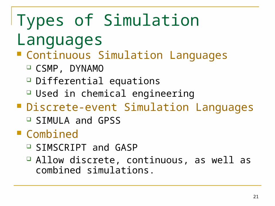
Types of Simulation Languages Continuous Simulation Languages

CSMP, DYNAMO Differential equations Used in chemical engineering

Discrete-event Simulation Languages SIMULA and GPSS

Combined SIMSCRIPT and GASP Allow discrete, continuous, as well as combined

simulations.

22

Types of Simulations

1. Emulation: Using hardware or firmware

2. Monte Carlo Simulation

3. Trace-Driven Simulation

4. Discrete Event Simulation

23

Types of Simulations (cont’d) Emulation

Simulation that runs on a computer to make it appear to be something else

Examples: JVM, NIST Net

Operating System

Hardware

Process Process

Java program

Java VM

24

Types of Simulation (cont’d)

Monte Carlo method [Origin: after Count Montgomery

de Carlo, Italian gambler and random-number

generator (1792-1838).] A method of jazzing up the

action in certain statistical and number-analytic

environments by setting up a book and inviting bets on

the outcome of a computation.

- The Devil's DP Dictionary

McGraw Hill (1981)

25

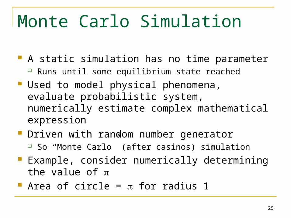
Monte Carlo Simulation

A static simulation has no time parameter Runs until some equilibrium state reached

Used to model physical phenomena, evaluate probabilistic system, numerically estimate complex mathematical expression

Driven with random number generator So “Monte Carlo” (after casinos) simulation

Example, consider numerically determining the value of

Area of circle = for radius 1

26

Monte Carlo Simulation (cont’d)

Imagine throwing dart at square Random x (0,1) Random y (0,1)

Count if inside sqrt(x2+y2) < 1

Compute ratio R in / (in + out)

Can repeat as many times as needed to get arbitrary precision

Unit square area of 1 Ratio of area in

quarter to area in square = R = 4R

27

Monte Carlo Simulation (cont’d) Evaluate the following integral

1. Generate uniformly distributed x ~ Uniform(0,2)

2. Density function f(x)=1/2 iff 0x 2

3. Compute:

28

Monte Carlo Simulation (cont’d) Expected value for y:

29

Trace-Driven Simulation

Uses time-ordered record of events on real system as input Example: to compare memory management, use

trace of page reference patterns as input, and can model and simulate page replacement algorithms

Note, need trace to be independent of system Example: if had trace of disk events, could not be

used to study page replacement since events are dependent upon current algorithm

30

Advantages of Trace-Driven Simulations1. Credibility2. Easy Validation: Compare simulation with measured3. Accurate Workload: Models correlation and interference 4. Detailed Trade-Offs: Detailed workload Can study small changes in algorithms5. Less Randomness: Trace deterministic input Fewer repetitions6. Fair Comparison: Better than random input7. Similarity to the Actual Implementation: Trace-driven model is similar to the system Can understand complexity of implementation

31

Disadvantages of Trace-Driven Simulations1. Complexity: More detailed

2. Representativeness: Workload changes with time, equipment

3. Finiteness: Few minutes fill up a disk

4. Single Point of Validation: One trace = one point

5. Detail

6. Trade-Off: Difficult to change workload

32

Discrete Event Simulations

A simulation using a discrete state model of the system is DISCRETE EVENT SIMULATION Continuous-event simulations – the state of the system takes

continuous values Typical components:

Event scheduler Simulation Clock and a Time Advancing Mechanism System State Variables Event Routines Input Routines Report Generator Initialization Routines Trace Routines Dynamic Memory Management Main Program

33

Components of Discrete Event Simulations Event scheduler – linked list of events waiting

Schedule event X at time T Hold event X for interval dt Cancel previously scheduled event X Hold event X indefinitely until scheduled by other event Schedule an indefinitely scheduled event Note, event scheduler executed often, so has significant impact

on performance Simulation Clock and a Time Advancing Mechanism

Global variable representing simulated time (maintained by the scheduler)

Two approaches Unit-time approach: increment time and check for events Event-driven approach: move to the next event in queue

34

Components of Discrete Events Sims (cont’d) System State Variable

Global variables describing the state of the systems(e.g., the umber of jobs in CPU scheduling simulation)

Local variables (e.g., CPU time required for a job is placed in the data structure for that particular job)

Event Routines -- one per event; update state variables and schedule other events E.g., job arrivals, job scheduling, and job departure

Input Routines Get model parameters

(e.g., means CPU time per job) from the user Very parameters in a range

35

Components of Discrete Events Sims (cont’d) Report Generator

Output routines run at the end of the simulation Initialization Routines

Set the initial state of the system state variables. Initialize seeds. Trace Routines

Print out intermediate variables as the simulation proceeds On/off feature

Dynamic Memory Management New entities are created and old ones are destroyed Periodic garbage collection

Main Program Tie everything together

36

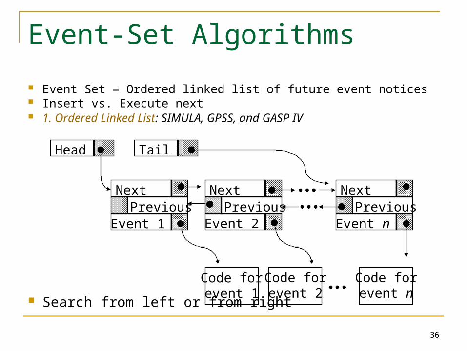
Event-Set Algorithms

Event Set = Ordered linked list of future event notices Insert vs. Execute next 1. Ordered Linked List: SIMULA, GPSS, and GASP IV

Search from left or from right

Head Tail

NextPrevious

Event n

NextPrevious

Event 1

NextPrevious

Event 2

Code forevent 1

Code forevent 2

Code forevent n

37

Event-Set Algorithms (cont’d) 2. Indexed Linear List

Array of indexes No search to find the sub-list Fixed or variable t. Only the first list is kept sorted

Head 1 Tail 1

Head 3 Tail 3

Head 2 Tail 2

t

t+ t

t+n t

38

Event-Set Algorithms (Cont)

3. Tree Structures: Binary tree log2 n Special case: Heap: Event is a node in binary tree

19

15

28

48

39 4527

34 50

23

25 47

(a) Tree representation of a heap.

1

2 3

4 5 6 7

8 9 10 11 12

39

Summary

Common Mistakes: Detail, Invalid, Short Discrete Event, Continuous time, nonlinear

models Monte Carlo Simulation: Static models Trace driven simulation: Credibility, difficult

trade-offs Even Set Algorithms: Linked list, indexed

linear list, heaps

Analysis of Simulation Results

41

Overview

Analysis of Simulation Results Model Verification Techniques Model Validation Techniques Transient Removal Terminating Simulations Stopping Criteria: Variance Estimation Variance Reduction

42

Model Verification vs. Validation The model output should be close to that of real system

Make assumptions about behavior of real systems 1st step, test if assumptions are reasonable

Validation, or representativeness of assumptions 2nd step, test whether model implements assumptions

Verification, or correctness

Four Possibilities1. Unverified, Invalid

2. Unverified, Valid

3. Verified, Invalid

4. Verified, Valid

43

Model Verification Techniques1. Top Down Modular Design2. Anti-bugging3. Structured Walk-Through4. Deterministic Models5. Run Simplified Cases6. Trace7. On-Line Graphic Displays8. Continuity Test9. Degeneracy Tests10. Consistency Tests11. Seed Independence

44

Top Down Modular Design

Divide and Conquer Modules = Subroutines, Subprograms,

Procedures Modules have well defined interfaces Can be independently developed, debugged, and

maintained Top-down design

Hierarchical structure Modules and sub-modules

45

Top Down Modular Design (cont’d)

Computer Network Simulator for Congestion Control studies

46

Top Down Modular Design (cont’d)

47

Verification Techniques

Anti-bugging: Include self-checks Probabilities = 1 Jobs left = Generated - Serviced

Structured Walk-Through Explain the code another person or group Works even if the person is sleeping

Deterministic Models: Use constant values Run Simplified Cases

Only one packet Only one source Only one intermediate node

48

Verification Techniques (cont’d) Trace = Time-ordered list of events and

variables Several levels of detail

Events trace Procedure trace Variables trace

User selects the detail Include on and off

49

Verification Techniques (cont’d) On-Line Graphic Displays

Make simulation interesting Help selling the results More comprehensive than trace

50

Verification Techniques (cont’d) Continuity Test

Run for different values of input parameters Slight change in input slight change in output

If not, investigate

Before After

51

Verification Techniques (cont’d) Degeneracy Tests: Try extreme

configuration and workloads One CPU, Zero disk

Consistency Tests Similar result for inputs that have same effect

Four users at 100 Mbps vs. Two at 200 Mbps Build a test library of continuity,

degeneracy and consistency tests Seed Independence: Similar results for

different seeds

52

Model Validation Techniques

Ensure assumptions used are reasonable Final simulated system should be like the real system

Unlike verification, techniques to validate one simulation may be different from one model to another

Three key aspects to validate Assumptions Input parameter values and distributions Output values and conclusions

Compare validity of each to one or more of Expert intuition Real system measurements Theoretical results

9 combinations- Not all are always possible, however

53

Expert Intuition

Most practical and common way Experts = Involved in design, architecture,

implementation, analysis, marketing, or maintenance of the system

Present assumption, input, output Better to validate one at a time See if the experts can distinguish simulation vs.

measurement

Th

roughput

0.2 0.4 0.8

Which alternativelooks invalid? Why?

54

Real System Measurements

Most reliable and preferred May be unfeasible because system does not exist or

too expensive to measure That could be why simulating in the first place!

But even one or two measurements add an enormous amount to the validity of the simulation

Should compare input values, output values, workload characterization Use multiple traces for trace-driven simulations

Can use statistical techniques (confidence intervals) to determine if simulated values different than measured values

55

Theoretical Results

Can be used to compare a simplified system with simulated results

May not be useful for sole validation but can be used to complement measurements or expert intuition E.g.: measurement validates for one processor, while analytic

model validates for many processors Note, there is no such thing as a “fully validated” model

Would require too many resources and may be impossible Can only show is invalid

Instead, show validation in a few select cases, to lend confidence to the overall model results

56

Transient Removal

Most simulations only want steady state Remove initial transient state

Trouble is, not possible to define exactly what constitutes end of transient state

Use heuristics: Long runs Proper initialization Truncation Initial data deletion Moving average of replications Batch means

57

Long Runs

Use very long runs Effects of transient state will be amortized But … wastes resources And tough to choose how long is “enough” Recommendation … don’t use long runs

alone

58

Proper Initialization

Start simulation in state close to expected state

Ex: CPU scheduler may start with some jobs in the queue

Determine starting conditions by previous simulations or simple analysis

May result in decreased run length, but still may not provide confidence that are in stable condition

59

Truncation

Assume variability during steady state is less than during transient state

Variability measured in terms of range (min, max)

If a trajectory of range stabilizes, then assume that in stable state

Method: Given n observations

{x1, x2, …, xn} Ignore first l observations Calculate (min,max) of

remaining n-l Repeat for l = 1…n Stop when l+1th

observation is neither min nor max

60

Truncation Example

Sequence: 1, 2, 3, 4, 5, 6, 7, 8, 9, 10, 11, 10, 9, 10, 11, 10, 9…

Ignore first (l=1), range is (2, 11) and 2nd observation (l+1) is the min

Ignore second (l=2), range is (3,11) and 3rd observation (l+1) is min

Finally, l=9 and range is (9,11) and 10th observation is neither min nor max

So, discard first 9 observations

TransientInterval

61

Truncation Example 2 (1 of 2) Find duration of transient interval for:

11, 4, 2, 6, 5, 7, 10, 9, 10, 9, 10, 9, 10

62

Truncation Example 2 (2 of 2) Find duration of

transient interval for:11, 4, 2, 6, 5, 7, 10, 9,

10, 9, 10, 9, 10 When l=3, range is

(5,10) and 4th (6) is not min or max

So, discard only 3 instead of 6

“Real” transient

Assumed transient

63

Initial Data Deletion (1 of 3)

Study average after some initial observations are deleted from sample If average does not change much, must be deleting from

steady state However, since randomness can cause some fluctuations

during steady state, need multiple runs (w/different seeds)

Given m replications size n each with xij – jth observation of ith replication Note j varies along time axis

and i varies across replications

64

Initial Data Deletion (2 of 3) Get mean trajectory:

xj = (1/m)xij j=1,2,…,n Get overall mean

x = (1/n)xj j=1,2,…,n Set l=1. Assume transient state l long, delete

first l and repeat for remaining n-lxl = (1/(n-l))xj j=l+1,…,n

Compute relative change

(xl – x) / x Repeat with l from 1 to n-1. Plot. Relative

change graph will stabilize at knee. Choose l there and delete 1 through l

65

Initial Data Deletion (3 of 3)

xij

j

xj

j

xl

l

(xl –

x)

/ x

l

transientinterval

knee

66

Moving Average of Independent Replications Compute mean over moving

time window Get mean trajectory

xj = (1/m)xij j=1,2,…,n Set k=1. Plot moving average

of 2k+1 values:Mean xj = 1/(2k+1) (xj+l)

With j=k+1, k+2,…,n-kWith l=-k to k

Repeat for k=2,3… and plot until smooth

Find knee. Value at j is length of transient phase.

xj

j

Mean

xj

j

transientinterval

knee

67

Batch Means

Run for long time N observations

Divide up into batches m batches size n each so m = N/n

Compute batch mean (xi) Compute var of batch means as

function of batch size (X is overall mean) Var(x) = (1/(m-1))(xi-X)2

Plot variance versus size n When n starts decreasing, have

transientR

esp

on

ses

Observation number

n 2n 3n 4n 5n

Vari

ance

of

batc

h m

eans

transientinterval

Batch size n

(Ignore)

68

Terminating Simulations For some simulations, transition state is of interest no

transient removals required Sometimes upon termination you also get final

conditions that do not reflect steady state Can apply transition removal conditions to end of simulation

Take care when gathering at end of simulation E.g.: mean service time should include only those that finish

Also, take care of values at event times E.g.: queue length needs to consider area under curve Say t=0 two jobs arrive, t=1 one leaves, t=4 2nd leaves qlengths q0=2, q1=1 q4=0 but q average not (2+1+0)/3=1 Instead, area is 2 + 1 + 1 + 1 so q average 5/4=1.25

69

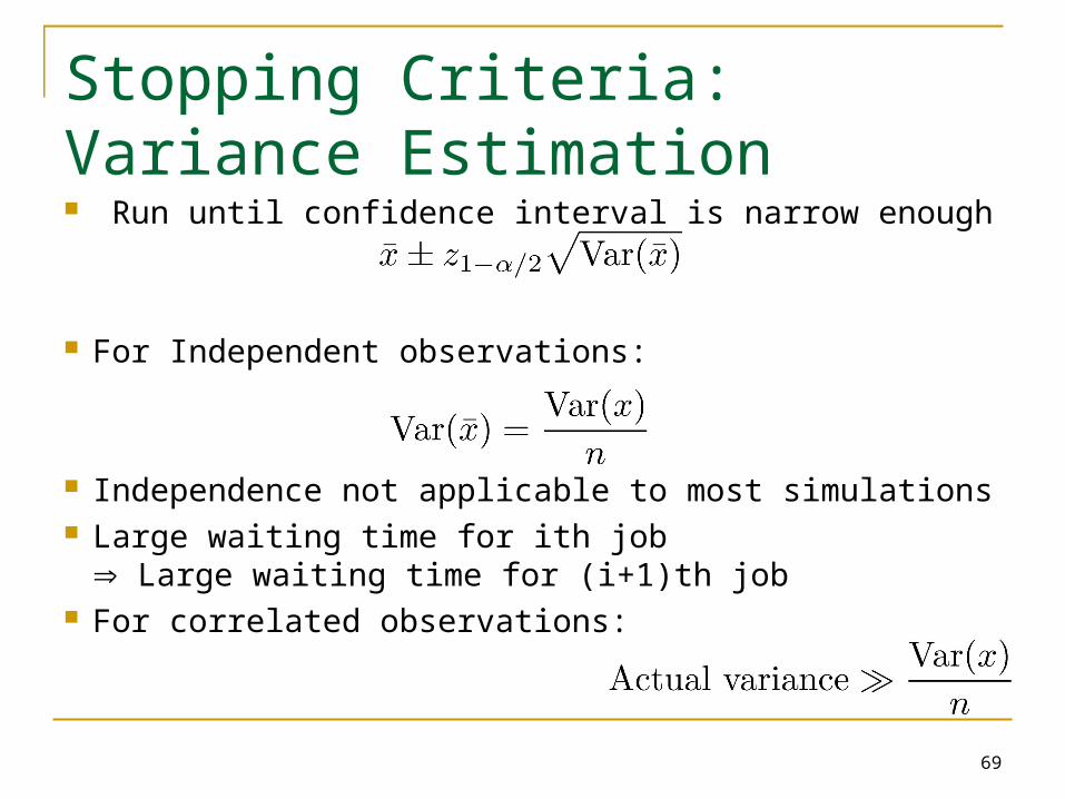
Stopping Criteria: Variance Estimation Run until confidence interval is narrow enough

For Independent observations:

Independence not applicable to most simulations Large waiting time for ith job

Large waiting time for (i+1)th job For correlated observations:

70

Variance Estimation Methods

1. Independent Replications

2. Batch Means

3. Method of Regeneration

71

Independent Replications

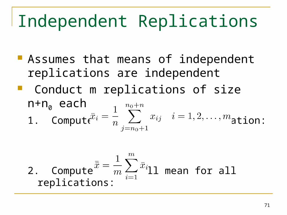
Assumes that means of independent replications are independent

Conduct m replications of size n+n0 each

1. Compute a mean for each replication:

2. Compute an overall mean for all replications:

72

Independent Replications (cont’d)3. Calculate the variance of replicate means:

4. Confidence interval for the mean response is:

Keep replications large to avoid waste Ten replications generally sufficient

73

Batch Means

Also called method of sub-samples Run a long simulation run Discard initial transient interval, and Divide the

remaining observations run into several batches or sub-samples. 1. Compute means for each batch:

2. Compute an overall mean:

74

Batch Means (cont’d)

3. Calculate the variance of batch means:

4. Confidence interval for the mean response is:

Less waste than independent replications Keep batches long to avoid correlation Check: Compute the auto-covariance of successive batch

means:

Double n until autocovariance is small

75

Case Study 25.1: Interconnection Networks Indirect binary n-cube networks:

Used for processor-memory interconnection Two stage network with full fan out. At 64, autocovariance

< 1% of sample variance

76

Method of Regeneration

Behavior after idle period does not depend upon the past history System takes a new birthRegeneration point

Note: The regeneration point are the beginning of the idle interval. (not at the ends as shown in the book).

Regeneration Points

QueueLength

77

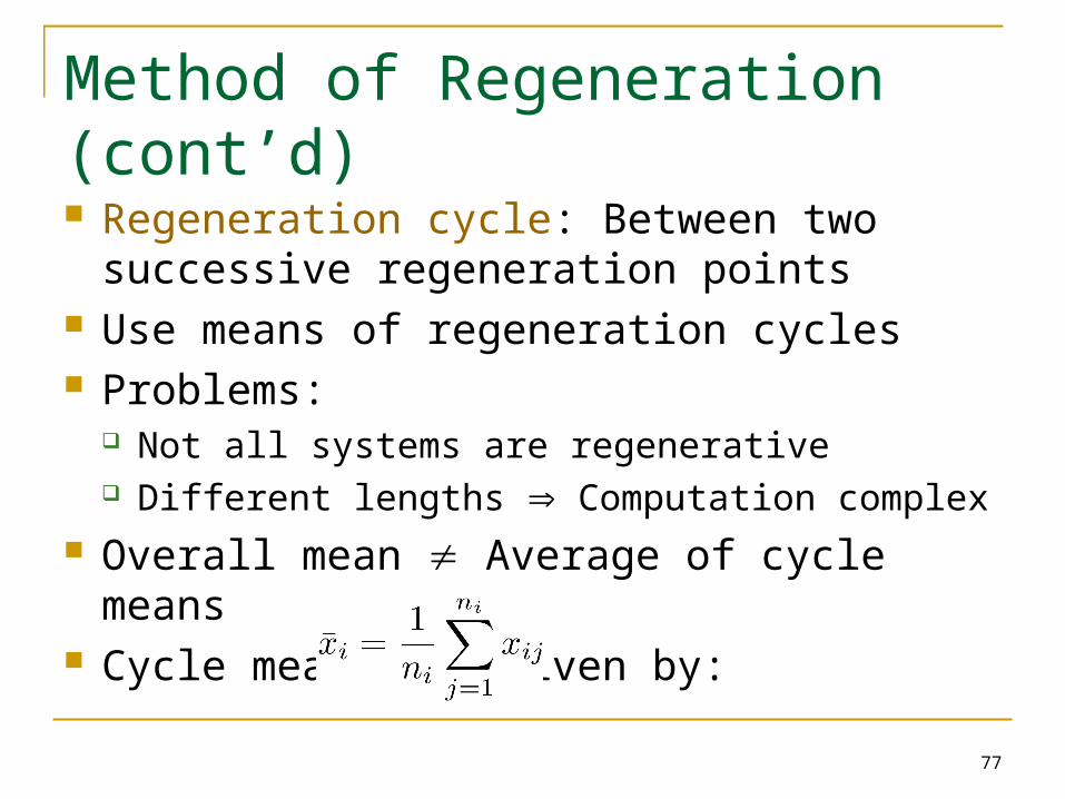
Method of Regeneration (cont’d) Regeneration cycle: Between two successive

regeneration points Use means of regeneration cycles Problems:

Not all systems are regenerative Different lengths Computation complex

Overall mean Average of cycle means Cycle means are given by:

78

Method of Regeneration (cont’d) Overall mean:

1. Compute cycle sums:

2. Compute overall mean:

3. Calculate the difference between expected and observed cycle sums:

79

Method of Regeneration (cont’d)4. Calculate the variance of the differences:

5. Compute mean cycle length:

6. Confidence interval for the mean response is given by:

7. No need to remove transient observations

80

Method of Regeneration: Problems1. The cycle lengths are unpredictable. Can't

plan the simulation time beforehand.

2. Finding the regeneration point may require a lot of checking after every event.

3. Many of the variance reduction techniques can not be used due to variable length of the cycles.

4. The mean and variance estimators are biased

81

Variance Reduction

Reduce variance by controlling random number streams

Introduce correlation in successive observations

Problem: Careless use may backfire and lead to increased variance.

For statistically sophisticated analysts only Not recommended for beginners

82

Summary

Verification = Debugging Software development techniques

Validation Simulation = Real Experts involvement

Transient Removal: Initial data deletion, batch means Terminating Simulations = Transients are of interest Stopping Criteria: Independent replications, batch

means, method of regeneration Variance reduction is not for novice