
Introduction to Machine Learning - UMIACS · Introduction to Machine Learning CMSC 422 Ramani...
27
Introduction to Machine Learning CMSC 422 Ramani Duraiswami Decision Trees Wrapup, Overfitting Slides adapted from Profs. Carpuat and Roth
Transcript of Introduction to Machine Learning - UMIACS · Introduction to Machine Learning CMSC 422 Ramani...

Introduction to Machine LearningCMSC 422
Ramani Duraiswami
Decision Trees Wrapup, Overfitting
Slides adapted from Profs. Carpuat and Roth
A decision tree to distinguish homes in
New York from homes in San
Francisco
http://www.r2d3.us/visual-intro-to-machine-learning-part-1/

Inductive bias in
decision tree learning
• Our learning algorithm
performs heuristic search
through space of decision
trees
• It stops at smallest acceptable
tree
• Why do we prefer small trees?
– Occam’s razor: prefer the
simplest hypothesis that fits
the data
Evaluating the learned hypothesis ℎ
• Assume
– we’ve learned a tree ℎ using the top-down
induction algorithm
– It fits the training data perfectly
• Is it guaranteed to be a good hypothesis?

Training error is not sufficient
• We care about generalization to new
examples
• A tree can classify training data perfectly,
yet classify new examples incorrectly
– Because training examples are incomplete --
only a sample of data distribution
• a feature might correlate with class by coincidence
– Because training examples could be noisy
• e.g., accident in labeling

Our training data
6
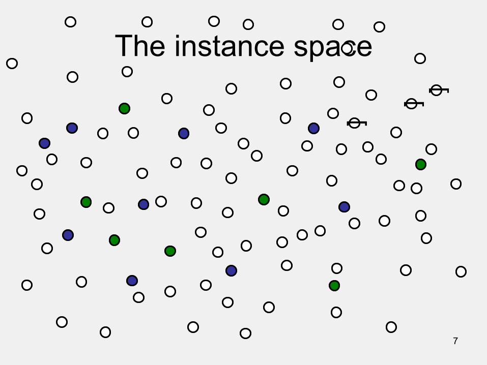
The instance space
]]
]]]]
7

Missing Values
8
Outlook
Overcast Rain
3,7,12,13 4,5,6,10,14
3+,2-
Sunny
1,2,8,9,11
4+,0-2+,3-
YesHumidity Wind
NormalHigh
No
WeakStrong
No YesYes
Outlook = ???, Temp = Hot, Humidity = Normal, Wind = Strong, label = ??
1/3 Yes + 1/3 Yes +1/3 No = Yes
Outlook = Sunny, Temp = Hot, Humidity = ???, Wind = Strong, label = ?? Normal/High
Other
suggestions?

Recall: Formalizing Induction
• Given
– a loss function 𝑙
– a sample from some unknown data distribution 𝐷
• Our task is to compute a function f that has low
expected error over 𝐷 with respect to 𝑙.
𝔼 𝑥,𝑦 ~𝐷 𝑙(𝑦, 𝑓(𝑥)) =
(𝑥,𝑦)
𝐷 𝑥, 𝑦 𝑙(𝑦, 𝑓(𝑥))
We end up reducing the error on the training
subset alone

Overfitting
• Consider a hypothesis ℎ and its:
– Error rate over training data 𝑒𝑟𝑟𝑜𝑟𝑡𝑟𝑎𝑖𝑛(ℎ)
– True error rate over all data 𝑒𝑟𝑟𝑜𝑟𝑡𝑟𝑢𝑒 ℎ
• We say ℎ overfits the training data if
𝑒𝑟𝑟𝑜𝑟𝑡𝑟𝑎𝑖𝑛 ℎ < 𝑒𝑟𝑟𝑜𝑟𝑡𝑟𝑢𝑒 ℎ
• Amount of overfitting =𝑒𝑟𝑟𝑜𝑟𝑡𝑟𝑢𝑒 ℎ − 𝑒𝑟𝑟𝑜𝑟𝑡𝑟𝑎𝑖𝑛 ℎ

Effect of Overfitting
in Decision Trees

Evaluating on test data
• Problem: we don’t know 𝑒𝑟𝑟𝑜𝑟𝑡𝑟𝑢𝑒 ℎ !
• Solution:
– we set aside a test set
• some examples that will be used for evaluation
– we don’t look at them during training!
– after learning a decision tree, we calculate
𝑒𝑟𝑟𝑜𝑟𝑡𝑒𝑠𝑡 ℎ

Underfitting/Overfitting
• Underfitting
– Learning algorithm had the opportunity to learn more
from training data, but didn’t
– Or didn’t have sufficient data to learn from
• Overfitting
– Learning algorithm paid too much attention to
idiosyncrasies of the training data; the resulting tree
doesn’t generalize
• What we want:
– A decision tree that neither underfits nor overfits
– Because it is expected to do best in the future

Pruning a decision tree
• Prune = remove leaves and assign
majority label of the parent to all items
• Prune the children of S if:
– all children are leaves, and
– the accuracy on the validation set does not
decrease if we assign the most frequent class
label to all items at S.
14

Avoiding Overfitting
• Two basic approaches
– Pre-pruning: Stop growing the tree at some point during construction
when it is determined that there is not enough data to make reliable
choices.
– Post-pruning: Grow the full tree and then remove nodes that seem not
to have sufficient evidence.
• Methods for evaluating subtrees to prune
– Cross-validation: Reserve hold-out set to evaluate utility
– Statistical testing: Test if the observed regularity can be dismissed as
likely to occur by chance
– Minimum Description Length: Is the additional complexity of the
hypothesis smaller than remembering the exceptions?
• This is related to the notion of regularization that we will see in other
contexts – keep the hypothesis simple.
15

Size of tree
Accuracy
On test data
On training data
Overfitting
• A decision tree overfits the training data when its accuracy on the training data goes up but its accuracy on unseen data goes down
16

Model complexity
Empirical
Error
Overfitting
17
• Empirical error (= on a given data set):
The percentage of items in this data set
are misclassified by the classifier f.
Model complexity
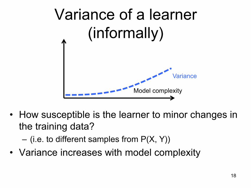
Variance of a learner
(informally)
• How susceptible is the learner to minor changes in
the training data?
– (i.e. to different samples from P(X, Y))
• Variance increases with model complexity
18
Variance

Model complexity
Bias of a learner (informally)
• How likely is the learner to identify the target hypothesis?
• Bias is low when the model is expressive (low empirical error)
• Bias is high when the model is (too) simple
– The larger the hypothesis space is, the easier it is to be close to the true
hypothesis.
19
Bias

Model complexity
Expected
Error
Impact of bias and variance
20
• Expected error ≈ bias + variance
Variance
Bias

Model complexity
Expected
Error
Model complexity
21
• Simple models: High bias and low variance
Variance
Bias
Complex models:
High variance and low bias

Underfitting Overfitting
Model complexity
Expected
Error
Underfitting and Overfitting
22
• Simple models: High bias and low variance
Variance
Bias
Complex models:
High variance and low bias
This can be made more accurate for some loss functions.
We will develop a more precise and general theory that
trades expressivity of models with empirical error

Expectation
• X is a discrete random variable with
distribution P(X):
• Expectation of X (E[X]), aka. the mean of X (μX)
E[X} = x P(X=x)X := μX
• Expectation of a function of X (E[f(X)])
E[f(X)} = x P(X=x)f(x)
• If X is continuous, replace sums with
integrals23
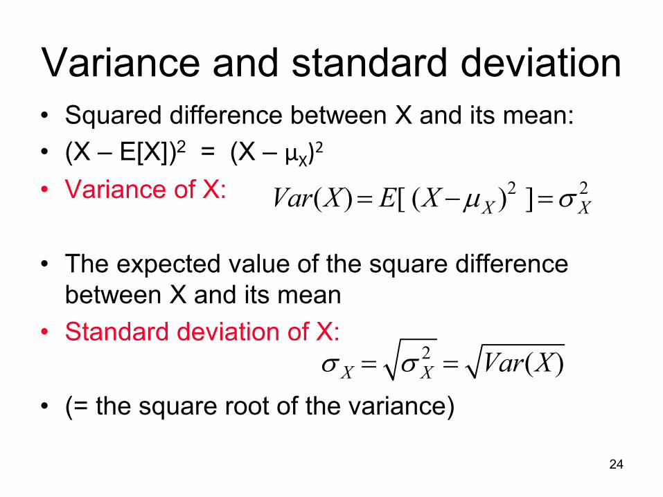
Variance and standard deviation• Squared difference between X and its mean:
• (X – E[X])2 = (X – μX)2
• Variance of X:
• The expected value of the square difference
between X and its mean
• Standard deviation of X:
• (= the square root of the variance)
24
Var(X)= E[ (X -mX )2 ]=s X
2
s X = s X2 = Var(X)

More on variance
• The variance of X is equal to the expected
value of X2 minus the square of its mean
• Var(X) = E[X2] − (E[X])2
= E[X2] − μX2
• Proof:
• Var(X) = E[(X − μX)2]
• = E[X2 − 2μXX + μX2]
• = E[X2] − 2μXE[X] + μX2
• = E[X2] − μX2
25

Train/dev/test sets
In practice, we always split examples into 3 distinct sets
• Training set
– Used to learn the parameters of the ML model
– e.g., what are the nodes and branches of the decision tree
• Development set
– aka tuning set, aka validation set, aka held-out data)
– Used to learn hyperparameters
• Parameter that controls other parameters of the model
• e.g., max depth of decision tree
• Test set
– Used to evaluate how well we’re doing on new unseen examples

Cardinal rule of machine learning:
Never ever touch
your test data!