Introduction to Localization (lecture 2) - Indico · 2018-11-22 · Introduction to Localization...

Introduction to Localization(lecture 2)

Stefano Cremonesi

Durham University

Bicocca-Surrey School “Prospects in Strings, Fields and Related Topics”University of Milano-Bicocca, 21/9/2018

Stefano Cremonesi Introduction to Localization (lecture 2)

SUSY on curved space and Localisation

We will see how the idea of localisation applies to the path integral of asupersymmetric quantum field theory on a compact curved manifoldM.

Compact space provides IR cutoff, making path integral better defined

Supersymmetric localisation reduces it to a finite-dimensional integral

ZM[J] =⟨

e−∫

JO⟩

=

∫[DX] e−S[X]−

∫JO

J is a supersymmetric source, coupled to a supersymmetric observable O.

The dependence onM is hidden in S[X] and the notion of supersymmetry.


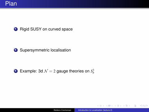
Plan

1 Rigid SUSY on curved space

2 Supersymmetric localisation

3 Example: 3d N = 2 gauge theories on S3b


Rigid SUSY on curved space


The problem of defining rigid SUSY on curved space

Supersymmetric QFT on flat space (Rd, g(0)µν = ηµν):

Flat space SUSY algebra

L(0) SUSY Lagrangian

Ü SUSY transformations δ(0)X

Ü δ(0)L(0) = ∂µ(. . . )µ

↓

Supersymmetric QFT on curved space (Md, gµν):

Curved space SUSY algebra

L SUSY Lagrangian

Ü SUSY transformations δX

Ü δL = ∇µ(. . . )µ

?

We would like to know:1 For which flat space SUSY algebras and (Md, gµν) this is possible2 What are δX and L(X, ∂µX)


Approach 1: Trial and error

δ = δ(0)∣∣ η→g∂→∇

+∑n≥1

1rn δ

(n)

L = L(0)∣∣ η→g∂→∇

+∑n≥1

1rnL

(n)

until SUSY algebra closes and δL = ∇µ(. . . )µ.

rM

Drawbacks:

- No guarantee it will work

- Case by case

- When it succeeds, expansions stop at n = 1 and n = 2 resp. Why?


Approach 2: Background supergravity [Festuccia, Seiberg 2011]

see also [Karlhede, Rocek 1988; Johansen 1995; Adams, Jockers, Kumar, Lapan 2011]

Nonlinearly couple supersymmetric FT to an off-shell supersymmetricbackground for supergravity multiplet (gµν , ψµα, aux).

Rigid limit of supergravity: gravity multiplet becomes non-dynamical.

Only require that the background is supersymmetric:

Generalised Killing spinor equations

ψµα = 0 , δζψµα = 0

Advantages:

- Model independent: only input is flat space SUSY algebra.

- δSuGra|bg XSFT = δXSFT , LSFT+SuGra|bg = LSFT .

- 1/r expansion above due to auxiliary fields.

- Supersymmetric backgrounds bg = (Md, gµν , aux, ζ) can be classified.


3d N = 2 SUSY with U(1)R symmetry

SUSY algebra on R3: Qα, Qβ = 2γµαβPµ + 2iεαβZ

Qα,Qβ = 0 Qα, Qβ = 0

[R,Qα] = −Qα [R, Qα] = +Qα

[Z,Qα] = [Z, Qα] = [Z,R] = 0

[Dumitrescu, Seiberg 2011]

Supercurrent R-multiplet: Tµν Sµα Sµα jµ(R) jµ(Z) iεµνρ∂ρJ(Z)

New min’l SUGRA multiplet: hµν ψµα ψµα Aµ Cµ Bµν

3d version of [Sohnius, West 1981/82]

Cµ ←→ Vµ = −iεµνρ∂µCρ Bµν ←→ H =i2εµνρ∂µBνρ

δLlinmin = −Tµνhµν −

12

Sµψµ +12

Sµψµ + jµ(R)(Aµ −32

Vµ) + jµ(Z)Cµ + J(Z)H


3d N = 2 SUSY with U(1)R symmetry onM3

[Klare, Tomasiello, Zaffaroni 2012; Closset, Dumitrescu, Festuccia, Komargodski 2012]

δζψµα, δζψµα in the rigid limit can be inferred from linear theory, diffeo + localR invariance and dimensional analysis, without knowing the full SuGra.

δζψµ = 2(∇µ − iAµ)ζ + Hγµζ + 2iVµζ + εµνρVνγρζ + (. . . )

δζψµ = 2(∇µ + iAµ)ζ + Hγµζ − 2iVµζ − εµνρVνγρζ + (. . . ) ,

(Generalised) Killing spinor equations

(∇µ − iAµ)ζ = −H2γµζ − iVµζ −

12εµνρVνγρζ

(∇µ + iAµ)ζ = −H2γµζ + iVµζ +

12εµνρVνγρζ .

Supersymmetric background:

(M3, gµν ,Aµ,Vµ,H) allowing solutions (ζ, ζ) 6= 0 of GKSE.


Curved space supersymmetry algebra

δζ , δζφ(r,z) = −2i(L′K + ζζ(z− rH)

)φ(r,z)

δζ , δηφ(r,z) = 0 δζ , δηφ(r,z) = 0

where L′K is a fully covariant Lie derivative along the Killing vector Kµ = ζγµζ,

L′Kϕ(r,z) =(KµDµ + i

2 (DµKν)Sµν)ϕ(r,z) ,

Dµϕ(r,z) =(∇µ − ir(Aµ − 1

2 Vµ)− izCµ)ϕ(r,z)

the totally covariant derivative of a field ϕ(r,z) of R-charge r and Z-charge z.

The representation of this SUSY algebra on a general multiplet is known.

We will be mostly interested in vector and chiral multiplets.


Vector multiplet V

SUSY transformations:

δaµ = −i(ζγµλ+ ζγµλ

)δσ = −ζλ+ ζλ

δλ = +ζ (D + iHσ)− i2εµνργρζ fµν − γµζ (iDµσ − Vµσ)

δλ = −ζ (D + iHσ)− i2εµνργρζ fµν + γµζ (iDµσ + Vµσ)

δD = Dµ(ζγµλ− ζγµλ

)− iVµ

(ζγµλ+ ζγµλ

)− H

(ζλ− ζλ

)SUSY Lagrangians:

LYM =1

g2YM

Tr(1

2fµν fµν + DµσDµσ + (D + iHσ)2 + iσεµνρVµfνρ − VµVµσ2

− 2iλγµ(Dµ + i2 Vµ)λ− 2iλ[σ, λ] + iHλλ

)LCS = i

k4π

Tr(εµνρ(aµ∂νaρ + i

23

aµaνaρ) + 2Dσ + 2λλ)

LFI = −iξ

2πTr (D− iHσ − iVµaµ)


Chiral multiplet Φ(r,z)

SUSY transformations:

δφ =√

2ζψ

δψ =√

2ζF −√

2i (z− σ − rH) ζφ−√

2iγµζDµφ

δF =√

2i (z− σ − (r − 2)H) ζψ + 2iζλφ

SUSY Lagrangians:

Lmat = DµφDµφ− iψγµDµψ − FF − iφVµDµφ

+ φ(− i(D + iHσ) + (z− σ − rH)2 + 2H(z− σ) +

r2

(12

R + VµVµ − H2))φ

+ iψ(

z− σ −(r − 1

2)H)ψ − 1

2ψγµVµψ +

√2i(φλψ + φλψ

)LW = FW(Φ) + FW(Φ) =

(F∂W∂φ

+ ψψ∂2W∂φ2

)+

(F∂W

∂φ+ ψψ

∂2W

∂φ2

)


Compact supersymmetric backgrounds

1 supercharge ζ: M3 has a transversely holomorphic foliation

Coordinates (τ, z, z): τ ′ = τ + t(z, z) , z′ = f (z) .

Metric: ds2 = (dτ + h(τ, z, z)dz + h(τ, z, z)dz)2 + c(τ, z, z)2dzdz

ζ determines all background fields, up to invariance of GKSE.

2 supercharges ζ, ζ: M3 is a Seifert manifold (S1 → M3 → Σ)

Metric: ds2 = Ω(z, z)2(dψ + h(z, z)dz + h(z, z)dz)2 + c(z, z)2dzdz

4 supercharges ζ1, ζ2, ζ1, ζ2:

T3

Round S2 × S1 with H = 0, A = V = ± iRS1

dτ [Imamura, S. Yokoyama 2011]

(Squashed) S3 with SU(2)× U(1) isometry: [Imamura, D. Yokoyama 2011]

ds2 = R2(

(µ1)2 + (µ2)2 + h2(µ3)2), H =

ihR, A = V = 2

√h2 − 1µ3


The 3d ellipsoid S3b [Hama, Hosomichi, Lee 2011]

b2|z1|2 + b−2|z2|2 = R2 S3 topology

U(1)2 isometry

z1 = Rb−1 sinϑ eiϕ1

z2 = Rb cosϑ eiϕ2

Background:

ds2 = R2(

b2 sin2 ϑ dϕ21 + b−2 cos2 ϑ dϕ2

2 + f (ϑ)2dϑ2)

H = − iRf (ϑ)

, 2A =

(1− b

f (ϑ)

)dϕ1 +

(1− b−1

f (ϑ)

)dϕ2

f (ϑ) = (b−2 sin2 ϑ+ b2 cos2 ϑ)1/2

ζ =1√2

(e

i2 (ϕ1+ϕ2+ϑ)

ei2 (ϕ1+ϕ2−ϑ)

), ζ =

1√2

(−e−

i2 (ϕ1+ϕ2−ϑ)

e−i2 (ϕ1+ϕ2+ϑ)

)Stefano Cremonesi Introduction to Localization (lecture 2)

Supersymmetric localisation


The path integral of a supersymmetric QFTConsider a supersymmetric QFT with fields X ∈ F :

Supercharge Q: Q2 = HAction S[X]: QS[X] = 0

Supersymmetric observable O: QO = 0

We wish to compute

〈O〉 =

∫F

[DX] O e−S[X]

Note that [Witten 1988]

〈QO′〉 =

∫F

[DX] (QO′)e−S[X] =

∫F

[DX] Q(O′e−S[X]

)= 0 ,

therefore expectation values only depend on the Q-cohomology class:

〈O +QO′〉 = 〈O〉


Localisation argument 1 [Witten 1991]

Assume the QFT has a symmetry group G which acts freely on field space F .For a G-invariant operator O,

〈O〉 =

∫F

[DX] O e−S[X] = Vol(G) ·∫F/G

[DX] O e−S[X] .

If G is generated by a fermionic charge Q, then Vol(G) ∝∫

dθ 1 = 0.

A supercharge Q does not act freely. Fixed points form the

BPS locus FQ = [X] ∈ F | fermions = 0, Q(fermions) = 0 .

If FQ,ε is an infinitesimal tubular neighbourhood of FQ of size ε,

〈O〉 = limε→0

(∫F\FQ,ε

[DX] O e−S[X] +

∫FQ,ε

[DX] O e−S[X]

)= limε→0

∫FQ,ε

[DX] O e−S[X]

Hence the path integral over field space F localises to the BPS locus FQ.


Localisation argument 2 [Witten 1988]

We can exploit the fact that the expectation value of a Q-closed observable Oonly depends on its Q-cohomology class [O]. Change representative:

〈O〉 = 〈O e−tQV[X]〉 =

∫F

[DX] O e−S[X]−tQV[X] ∀ t, V[X] s.t. Q2V[X] = 0 .

We will assume that ReQV[X]|bos is positive semi-definite and consider t ≥ 0.

〈O〉 = limt→+∞

∫F

[DX] O e−S[X]−tQV[X] .

t→ +∞: integral dominated by the saddle points of the

Localising action Sloc[X] = QV[X] ,

Localisation locus Floc = X0 ∈ F|δSloc[X]

δX

∣∣∣X0

= 0 .


Exact semiclassical approximation in ~aux = 1/t, around saddles X0 of Sloc:

X = X0 +1√

tδX

S[X] + tSloc[X] −−−−→t→+∞

S[X0] +12

x δ2Sloc[X]

δX2

∣∣∣X0

(δX)2

Integrating out the transverse fluctuations δX, one obtains

Localisation formula

〈O〉 =

∫Floc

[DX0] O|X0 e−S[X0]1

Sdet[δ2Sloc[X0]

δX20

] .

E.g., for the standard choice (here Ψ = fermions) [Pestun 2007]

VP = (QΨ,Ψ) =⇒ Sloc|bos = (QΨ,QΨ) ≥ 0 ,

the path integral over F localizes to Floc = FQ, the BPS locus.Stefano Cremonesi Introduction to Localization (lecture 2)

The 1-loop determinant Z1−loop

Z1−loop = Sdet[δ2Sloc[X0]

δX20

]=

(det Kferm

det Kbos

)1/2

,

where the kinetic operators for bosonic and fermionic fluctuations Kbos, Kferm

are some modified Laplace and Dirac operators.

General observations:

Computing their spectrum can be difficult.

Many cancellations because SUSY pairs bosons and fermions.

One can localise to fixed points of Q2 in spacetime.

The computation is best done by organising fields cohomologically(i.e. in multiplets of Q) and applying index theorems. [Pestun 2007]


1 Reorganise fields in Q-multiplets X = φ, ψ′ = Qφ, ψ, φ′ = Qψ:

Qφ = ψ′ , Qψ′ = Q2φ .

Qψ = φ′ , Qφ′ = Q2ψ .

For simplicity,[Hosomichi 2015]

VH = (φ,Qφ) + (ψ,Qψ)

QVH = (ψ′, ψ′) + (φ,Q2φ) + (φ′, φ′)− (ψ,Q2ψ)

Z1−loop =

(detψQ2

detφQ2

)1/2

2 If there is a differential operator D that commutes with Q2,

D : Γ(E0) → Γ(E1)3 3φ ψ

D† : Γ(E1) → Γ(E0)3 3

ψ φ

then

Z1−loop =

(detcokerDQ2

detkerDQ2

)1/2

.← unpaired ψ← unpaired φ


The 1-loop determinant can be deduced from the Q2-equivariant index of D

Ind(D; eQ2) := trkerD(eQ

2)− trcokerD(eQ

2) =

∑j

dj ehj

as

Z1−loop =

(detcokerDQ2

detkerDQ2

)1/2

=∏

j

h−dj/2j .

If D is transversally elliptic, which ensures that dj are finite, the equivariantindex can be computed by the Atiyah-Bott fixed point formula e.g. [Atiyah 1974]

Ind(D; eQ2) =

∑p|eQ2 ·p=p

trE0(p) eQ2− trE1(p) eQ

2

detTM(p)(1− eQ2 ).

This reduces the computation of Z1−loop to determining the local action of Q2

around fixed points in field space F and in spacetimeM.


Localisation of 3d N = 2 gauge theories on S3b

[Hama, Hosomichi, Lee 2011], building on [Kapustin, Willett, Yaakov ’09; Jafferis ’10; HHL ’10]

Z[V] =

∫[DV][DΦ][DΦ] e−(SYM [V]+SCS[V]+SFI [V]+Smat[Φ,Φ,V,V]+SW [Φ,Φ])

V: background vector multiplet (global symmetry)

Localising supercharge: Q = δζ + δζ

Localising action: Sloc = QVP , VP =∑

Ψ∈λ,λ,ψ,ψ(QΨ,Ψ)

Localisation locus FQ: D = −iHσ, aµ = 0, σ = const.φ = φ = F = F = 0

Classical action: S[X0] = −ikπ tr(Rσ)2 + 2πi(ξR) tr(Rσ)

[SYM, Smat, SW are Q-exact] Zclass = eikπ tr(Rσ)2−2πi(ξR) tr(Rσ)


Diagonalise σ = σiHi: |J| =∏

α∈∆+

α(Rσ)2

1-loop det of Φ(r,z): ZΦ1−loop =

∞∏m,n=0

(m + 1)b + (n + 1)b−1 + iRzCmb + nb−1 − iRzC

“ = ”Γh(RzC)

RzC = Rz + ib + b−1

2r , z = ρ(σ) + ρ(σ)

1-loop det of V: ZV1−loop =

∏α∈∆+

4 sinh(πbα(Rσ)) sinh(πb−1α(Rσ))

α(Rσ)2

Coulomb branch localisation formula (R = 1)

ZS3b(σ; k, ξ, r) =

1|WG|

∫ rk(G)∏i=1

dσi Zclass(σ; ξ, k) Z1−loop(σ, σ, r) .

This result generalizes to any background with S3 topology: b ∈ C is themodulus of the transversely holomorphic foliation on S3.

[Closset, Dumitrescu, Festuccia, Komargodski 2013; Alday, Martelli, Richmond, Sparks 2013]


An alternative: Higgs branch localisation[Benini, SC ’12] in 2d; [Fujitsuka, Honda, Yoshida ’13; Benini, Peelaers ’13] in 3d; ...

Localising action: S′loc = Q (VP + VHiggs)

VHiggs =

∫d3x√

g tr( ζλ− ζλ

2iM(φ, φ)

)M(φ, φ) =

∑α

φαφ†α − ξ , ξ =∑

i∈Cartan(g)

ξihi

When the “fake FI parameter” ξ →∞ (in an appropriate direction):

Coulomb branch saddles are suppressed

Higgs branch saddles controlled by M (plus zero size vortices) dominate.

Higgs branch localisation formula

Z =∑

Higgs vacua

Zclass Z′1−loop Z(NP)v Z(SP)

av

proving the factorisation of Z observed in [Pasquetti ’11], [Beem, Dimofte, Pasquetti ’12].Stefano Cremonesi Introduction to Localization (lecture 2)

Bonus tracks: two applications


Partition function and field theory dualitiesThe partition function ZM(V;λ) computed exactly by localisation allowsdetailed tests of field theory dualities. If theory A is dual to theory B, then

Z(A)M (V(A);λ(A)) = Z(B)

M (V(B);λ(B))

with a duality map

V(A)a =

∑b

cabV(B)

b

λ(A) = f (λ(B)) .

These tests have been performed for a variety of theories:[Dolan, Osborn ’08; Spiridonov, Vartanov ’08-’12; Kapustin, Willett, Yaakov ’10; Willett, Yaakov ’11;

Benini, Closset, SC ’11; Benini, SC ’12; Doroud, Gomis, Le Floch, Lee ’12; . . . ]

Identities between integrals of special functions

Useful to determine the duality map

Can be extended to supersymmetric operators


The free energy of 3d N = 2 SCFTs

A particularly interesting quantity for a 3d CFT:

Free energy F = − log ZS3 |finite

3d analogue of c and a central charges: it counts degrees of freedom.

It can be computed exactly using localisation for N ≥ 2 theories.

Using the large-N limit of the matrix model for ZS3 , it was shown thatM2-brane theories have F ∝ N3/2. [Drukker, Mariño, Putrov 2010]

F-maximisation: the N = 2 superconformal R-symmetry

R(t) = R0 +∑

a

taQa

maximizes Re(F(t)). [Jafferis 2010; Closset, Dumitrescu, Festuccia, Seiberg 2012]

F-theorem: F decreases along RG-flows. [Jafferis, Klebanov, Pufu, Safdi 2011][Casini, Huerta 2012]


Conclusions


Localisation has led to many exact results for broad classes ofsupersymmetric QFTs on curved manifolds of various dimensions.

What about 4d N = 1?

- S3 × S1 3

- Σg × T2 3

- S4 7

I have overlooked many interesting results: (Sorry!)

- “Superconformal” indices: ZSd−1×S1 = Tr (−1)Fe−β′Q,S−β

∑a vaFa

- Twisted partition functions

- Localisation on manifolds with boundaries

- Inclusion of order/disorder operators

- Even localisation of supersymmetric quantum theories of gravity!


Localisation will remain an important tool in the future:

Very concrete approach to make exact calculations in SUSY QFT.

Probes generic (strongly coupled) regimes of parameter/moduli space.

Allows to address fundamental questions in QFT and String Theory.

Many open questions, likely new directions are waiting to be explored.


Thank you for your attention!


Introduction to Localization (lecture 2) - Indico · 2018-11-22 · Introduction to Localization...

Documents

Transcript of Introduction to Localization (lecture 2) - Indico · 2018-11-22 · Introduction to Localization...