Introduction to Interrupted Time Series Part II. … to Interrupted Time Series Part II. Analysis...
27
SGregorich CAPS/TAPS January, 19, 2016 1 Introduction to Interrupted Time Series Part II. Analysis Options Joint CAPS/TAPS Methodology Seminar January 19, 2016 Steve Gregorich
Transcript of Introduction to Interrupted Time Series Part II. … to Interrupted Time Series Part II. Analysis...

SGregorich CAPS/TAPS January, 19, 2016 1
Introduction to Interrupted Time Series
Part II. Analysis Options
Joint CAPS/TAPS Methodology Seminar
January 19, 2016
Steve Gregorich
SGregorich CAPS/TAPS January, 19, 2016 2
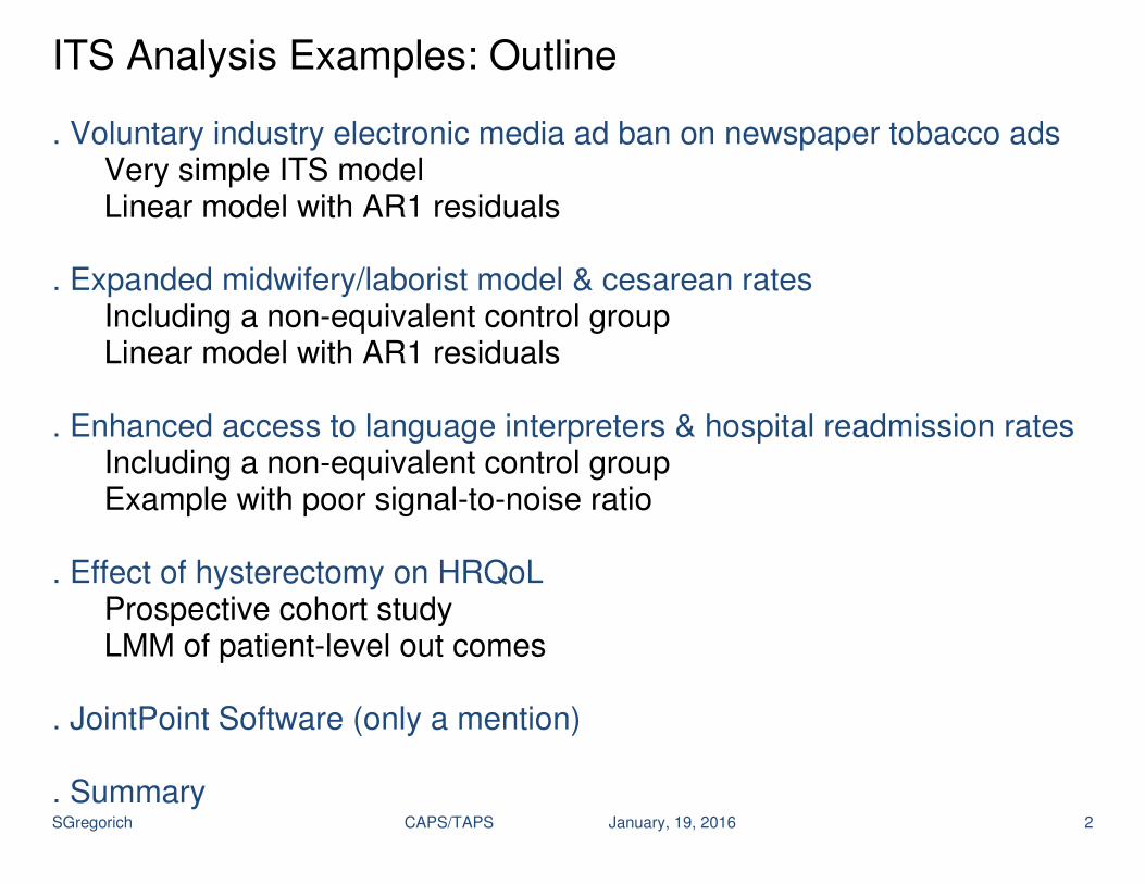
ITS Analysis Examples: Outline . Voluntary industry electronic media ad ban on newspaper tobacco ads Very simple ITS model Linear model with AR1 residuals . Expanded midwifery/laborist model & cesarean rates Including a non-equivalent control group Linear model with AR1 residuals . Enhanced access to language interpreters & hospital readmission rates Including a non-equivalent control group Example with poor signal-to-noise ratio . Effect of hysterectomy on HRQoL Prospective cohort study LMM of patient-level out comes . JointPoint Software (only a mention) . Summary

SGregorich CAPS/TAPS January, 19, 2016 3
Units of observation Unit(s) of observation observed across time a. A single unit observed longitudinally: a patient, a hospital, a county
b. Multiple units observed longitudinally: longitudinal cohort sample
c. Multiple cross sectional samples of individual units (with perhaps some individual units observed more than once) You may choose to aggregate data to a higher level of abstraction, e.g., Single unit observed:
daily summaries → monthly summaries
Multiple units observed:
patient-level outcomes in real time → monthly summaries

SGregorich CAPS/TAPS January, 19, 2016 4
ITS: Tobacco Ad Images in Argentinean Newspapers Beginning in the late 1980s, the tobacco industry anticipated increased anti-smoking pressure In 1997, the tobacco industry created a ‘weak’ voluntary ad ban Ads OK’d on radio and TV from 10PM to 8AM, only In 2000, the tobacco industry withdrew all ads from radio and TV Q: How did the 2000 radio and TV ban affect ads in the print media?

SGregorich CAPS/TAPS January, 19, 2016 5
2011. CVD Prevention & Control, 6, 71-80.
Objective: Describe prevalence of tobacco-related images and articles
Design . Observation period 1995-2004
. Industry self-imposed radio/TV ban in 2001
. 4 main national newspapers
. 4 sampled months per year March, June, August, November

SGregorich CAPS/TAPS January, 19, 2016 6
ITS: Tobacco Ad Images in Argentinean Newspapers Basic Results
. N=4828 newspaper issues sampled
. N=1800 tobacco-related images or articles identified
. n=360 articles
. n=1283 non-advisement images
. n=157 advertisement images Data aggregation
. Data were aggregated up to calendar year . Aggregated across newspapers w/in each year
. This was done by primary authors, other options possible
. Sample size: N=10 calendar years (1995-2004)

SGregorich CAPS/TAPS January, 19, 2016 7
ITS: Tobacco Ad Images in Argentinean Newspapers

SGregorich CAPS/TAPS January, 19, 2016 8
ITS: Tobacco Ad Images in Argentinean Newspapers Data
Year Year_Rel Ban Ad_Images Subj 1995 -6 0 16 1 1996 -5 0 24 1 1997 -4 0 18 1 1998 -3 0 5 1 1999 -2 0 13 1 2000 -1 0 3 1 2001 0 1 2 1 2002 +1 1 14 1 2003 +2 1 31 1 2004 +3 1 32 1
Code intervention onset as time=0

SGregorich CAPS/TAPS January, 19, 2016 9
ITS: Tobacco Ad Images in Argentinean Newspapers
Analysis plan
. Preliminary analyses suggested that annual counts were reasonably symmetrically distributed
. Modeled via linear regression with AR1 residuals
proc mixed data= Newspaper;
class Subj;
model Ad_Image = Year_Rel|Ban / s;
estimate 'post-slope' Year_Rel 1 Year_Rel*Ban 1;
repeated / subject= Subj type=AR(1);
run;
. Estimated intercept represents outcome level just prior to the ad ban
. Estimated effect of Ban represents ‘immediate effect’ of Ban . Model estimates separate slopes for pre- and post- periods
SGregorich CAPS/TAPS January, 19, 2016 10
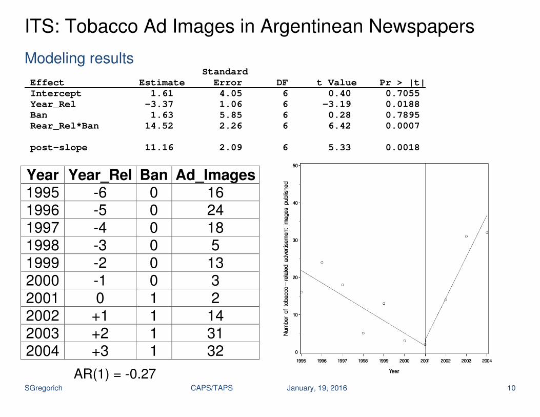
ITS: Tobacco Ad Images in Argentinean Newspapers
Modeling results Standard
Effect Estimate Error DF t Value Pr > |t|
Intercept 1.61 4.05 6 0.40 0.7055
Year_Rel -3.37 1.06 6 -3.19 0.0188
Ban 1.63 5.85 6 0.28 0.7895
Rear_Rel*Ban 14.52 2.26 6 6.42 0.0007
post-slope 11.16 2.09 6 5.33 0.0018
Year Year_Rel Ban Ad_Images 1995 -6 0 16 1996 -5 0 24 1997 -4 0 18 1998 -3 0 5 1999 -2 0 13 2000 -1 0 3 2001 0 1 2 2002 +1 1 14 2003 +2 1 31 2004 +3 1 32
AR(1) = -0.27
SGregorich CAPS/TAPS January, 19, 2016 11
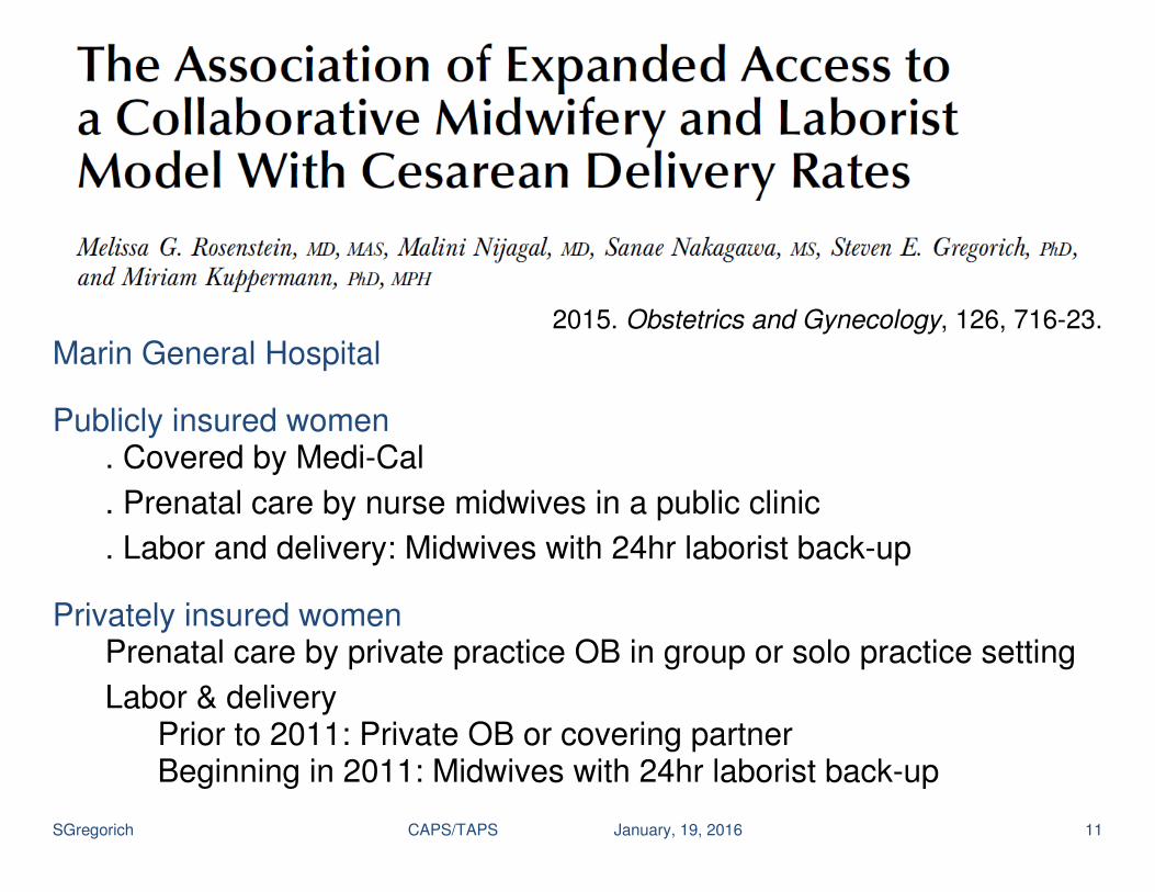
2015. Obstetrics and Gynecology, 126, 716-23.
Marin General Hospital
Publicly insured women . Covered by Medi-Cal
. Prenatal care by nurse midwives in a public clinic
. Labor and delivery: Midwives with 24hr laborist back-up
Privately insured women Prenatal care by private practice OB in group or solo practice setting
Labor & delivery Prior to 2011: Private OB or covering partner Beginning in 2011: Midwives with 24hr laborist back-up
SGregorich CAPS/TAPS January, 19, 2016 12
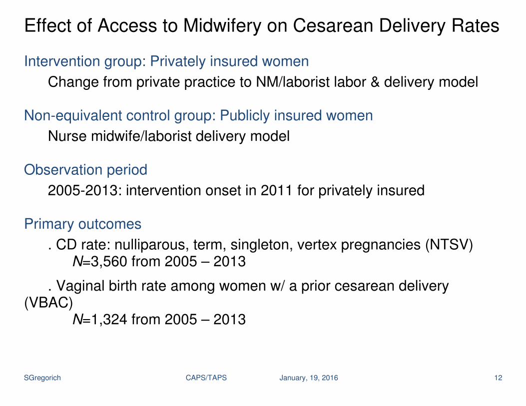
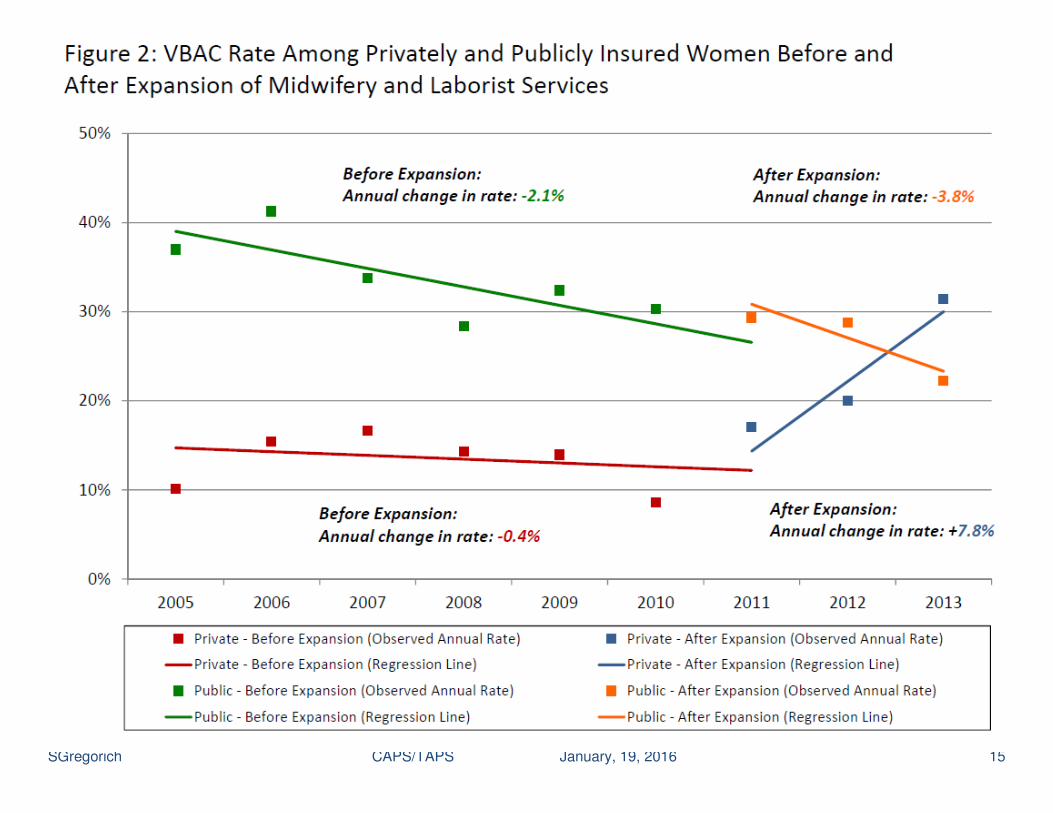
Effect of Access to Midwifery on Cesarean Delivery Rates Intervention group: Privately insured women
Change from private practice to NM/laborist labor & delivery model Non-equivalent control group: Publicly insured women
Nurse midwife/laborist delivery model Observation period
2005-2013: intervention onset in 2011 for privately insured Primary outcomes
. CD rate: nulliparous, term, singleton, vertex pregnancies (NTSV) N=3,560 from 2005 – 2013
. Vaginal birth rate among women w/ a prior cesarean delivery (VBAC) N=1,324 from 2005 – 2013

SGregorich CAPS/TAPS January, 19, 2016 13
Effect of Access to Midwifery on Cesarean Delivery Rates
Analysis Notes
We had access to patient-level outcomes
We aggregated up to annual rates (%)
Linear regression with AR1 residual correlation structure
The first author felt that reporting linear regression parameters representing expected changes in outcome prevalence (%) would be more accessible to readers
We could have modeled patient-level binary outcomes via GEE or GLMM Or, we could have modeled aggregated outcomes as a binomial. In those cases, we would have reported ORs versus linear reg. coeffs.
It would also be possible to model aggregated counts of CDs via, e.g., a negative binomial model, including an offset
With patient-level outcomes, you would not attempt to model AR1 resids. You could cluster repeated deliveries within patients (VBAC outcome), if any parous women delivered more than once during the study

SGregorich CAPS/TAPS January, 19, 2016 14
SGregorich CAPS/TAPS January, 19, 2016 15
SGregorich CAPS/TAPS January, 19, 2016 16
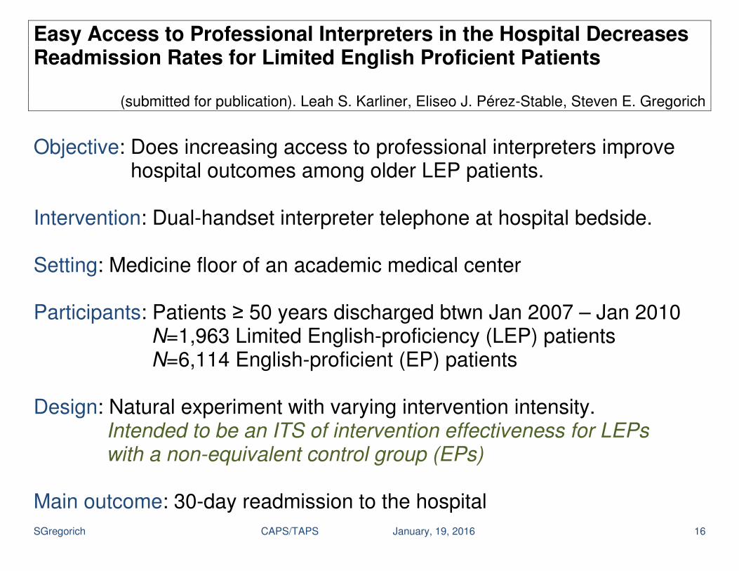
Easy Access to Professional Interpreters in the Hospital Decreases Readmission Rates for Limited English Proficient Patients
(submitted for publication). Leah S. Karliner, Eliseo J. Pérez-Stable, Steven E. Gregorich Objective: Does increasing access to professional interpreters improve hospital outcomes among older LEP patients. Intervention: Dual-handset interpreter telephone at hospital bedside. Setting: Medicine floor of an academic medical center Participants: Patients ≥ 50 years discharged btwn Jan 2007 – Jan 2010 N=1,963 Limited English-proficiency (LEP) patients N=6,114 English-proficient (EP) patients Design: Natural experiment with varying intervention intensity. Intended to be an ITS of intervention effectiveness for LEPs with a non-equivalent control group (EPs) Main outcome: 30-day readmission to the hospital
SGregorich CAPS/TAPS January, 19, 2016 17
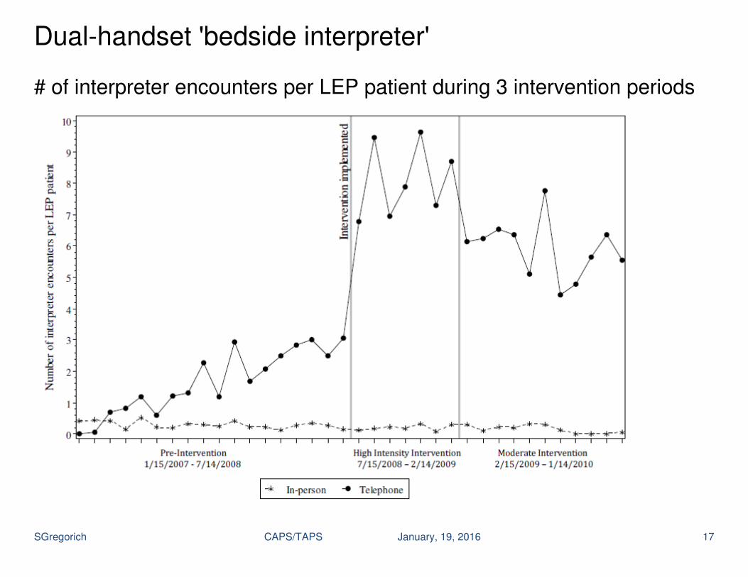
Dual-handset 'bedside interpreter' # of interpreter encounters per LEP patient during 3 intervention periods
SGregorich CAPS/TAPS January, 19, 2016 18
Dual-handset 'bedside interpreter' study Intended as an ITS design with 3 intervention periods: Pre-intervention, High-intensity intervention, Moderate intervention. Patient-level data were available We explored time trends of…
. Patient-level outcomes in continuous time
. Patient outcomes aggregated to calendar months ( 55 LEP; 170 EP)
. Patient outcomes aggregated to calendar quarter (164 LEP; 510 EP) Any trend signals within intervention periods were swamped by noise Eventually, we gave up on modeling trends within intervention periods We modeled patient-level data and estimated readmission probabilities
within the 3 intervention periods and whether the intervention effect was modified by language group (a 2-way ANCOVA model)

SGregorich CAPS/TAPS January, 19, 2016 19
Dual-handset 'bedside interpreter' study Results: 30-day readmission rates from N=7389 discharges Pre-
Intervention High
Intensity Intervention
Moderate Intensity
Intervention LEP
17.8%
(n=938)
13.4%
(n=365)
20.3%
(n=493)
EP
16.7%
(n=2931)
19.7%
(n=1209)
17.6%
(n=1453)

SGregorich CAPS/TAPS January, 19, 2016 20
Effect of hysterectomy on HRQoL
2013. Obstetrics & Gynecology, 122, 15-25
Prospective cohort study: N = 1503 women, up to 8 years FU
. Pre menopausal women: aged 31-54 (mean = 42.5) at baseline
. Sought care in the previous year for pelvic pain, abnormal uterine bleeding, and/or fibroids
. No cancer of the reproductive tract, intact uterus
. English or Spanish speakers

SGregorich CAPS/TAPS January, 19, 2016 21
Effect of hysterectomy on HRQoL Pre- and post-surgical HRQOL observations
. n=205 women had a hysterectomy sometime during the study
.Observation times were centered around the time of surgical intervention Ranged from -8 to +8 years, but we restricted to -4 through +7 Main HRQoL outcome . Perceived resolution of pelvic problems (PRPP) (1=not at all, 2=somewhat, 3=mostly, 4=completely)

SGregorich CAPS/TAPS January, 19, 2016 22
Effect of hysterectomy on HRQoL A smoothing spline model to explore the average trajectory
proc glimmix data= Mydata;
model Dv = Time;
random Time /
subject=intercept type=rsmooth;
output out= Smooth pred= Dv_hat;
run;
SGregorich CAPS/TAPS January, 19, 2016 23
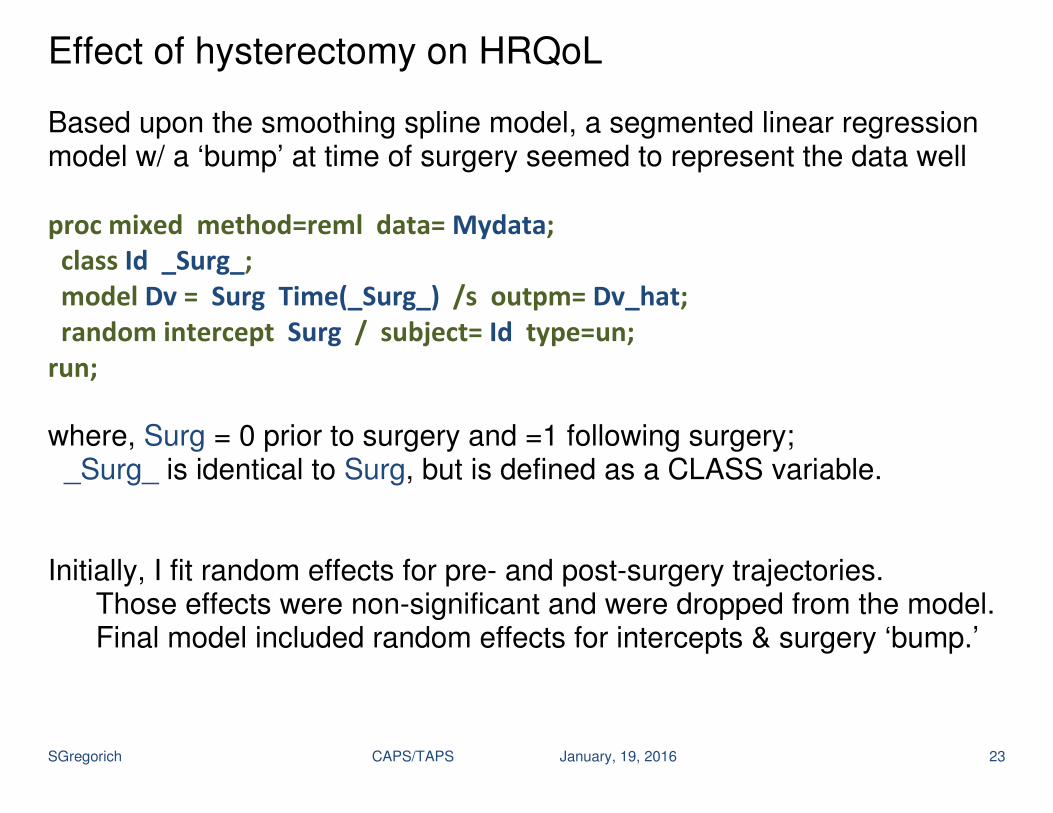
Effect of hysterectomy on HRQoL Based upon the smoothing spline model, a segmented linear regression model w/ a ‘bump’ at time of surgery seemed to represent the data well proc mixed method=reml data= Mydata;
class Id _Surg_;
model Dv = Surg Time(_Surg_) /s outpm= Dv_hat;
random intercept Surg / subject= Id type=un;
run;
where, Surg = 0 prior to surgery and =1 following surgery; _Surg_ is identical to Surg, but is defined as a CLASS variable. Initially, I fit random effects for pre- and post-surgery trajectories. Those effects were non-significant and were dropped from the model. Final model included random effects for intercepts & surgery ‘bump.’

SGregorich CAPS/TAPS January, 19, 2016 24
Effect of hysterectomy on HRQoL
Component Est.
VAR(int) 0.25
VAR(bump) 0.59
COV(i,b) -0.26
(r = -0.69)
VAR(res) 0.35
------------------------- post- v pre-HYST slopes,
∆ = 0.16** ------------------------- intercept = 1.45
B = 2.01***
B = -0.17***
B = -0.01
SGregorich CAPS/TAPS January, 19, 2016 25
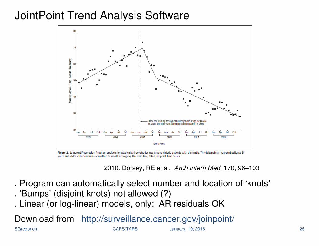
JointPoint Trend Analysis Software 2010. Dorsey, RE et al. Arch Intern Med, 170, 96–103
. Program can automatically select number and location of ‘knots’
. ‘Bumps’ (disjoint knots) not allowed (?)
. Linear (or log-linear) models, only; AR residuals OK
Download from http://surveillance.cancer.gov/joinpoint/

SGregorich CAPS/TAPS January, 19, 2016 26
Summary
Impact of unit of analysis on modeling options With one observation per time point
Linear models with AR1 residuals
Other GLMs possible, e.g., logistic or count outcome models With multiple observations per time point
. Linear or logistic models can be fit
. Account for repeated observations of the same unit: GEE/GLMM
. Account for clustering of observations, if any Covariates at same level of abstraction as outcomes (or higher)
If you aggregate outcome data, you’ll also aggregate covariates
When modeling patient-level or monthly aggregate outcome, consider including a covariate indicating calendar month (or quarter, if outcomes aggregated to that level)

SGregorich CAPS/TAPS January, 19, 2016 27
Summary
Impact of unit of analysis on modeling options
. When aggregating multi-unit data with binary outcomes you have choices regarding how to define the outcome
. mean response (proportion)
. median
. binomial or count outcome with denominator as ‘offset’
Other thoughts
. When modeling aggregated outcomes,
Center time variable: time=0 when intervention is first implemented
Intervention indicator = 0 prior to intervention; =1 during intervention
Grand-mean center covariates
This allows for most straightforward interpretation of parameters
With a few small tweaks, models that you are already familiar with can useful for analysis of data from ITS designs with short series
END