Chapter 1

Introduction

This thesis involves the development and application of adjoint methods to the seismic

tomographic inverse problem. The success of an inverse problem depends primarily on the

quality and coverage of the data, and on the accuracy of the forward modeling tool within the

inverse problem. Our forward modeling tool is the spectral-element method (SEM), which

has been developed for regional and global scales of seismic wave propagation (Komatitsch

and Vilotte, 1998; Komatitsch and Tromp, 2002a,b; Komatitsch et al., 2004).

The remaining chapters emphasize the inverse problem, so we will briefly state the

essential equations of the forward problem of seismic wave propagation. The equation of

motion for an anelastic Earth is given by

ρ∂2

s

∂t2= ∇ ·T + f , (1.1)

where ρ(x) denotes the density distribution, s(x, t) the seismic wavefield, T(x, t) the stress

tensor, and f(x, t) the earthquake source. (We neglect rotation and self-gravitation.)

If the medium is elastic, then we apply Hooke’s law

T = c : ∇s , (1.2)

which states that the stress is linearly related to the displacement gradient ∇s (strain)

through the fourth-order elastic tensor c(x).

1

CHAPTER 1. Introduction 2

If the elastic medium is isotropic, then the elements of c are described by two parameters:

cjklm = (κ − 23µ)δjkδlm + µ(δjlδkm + δjmδkl), (1.3)

where µ(x) is the shear modulus and κ(x) is the bulk modulus.

In general, the SPECFEM3D software (Komatitsch and Tromp, 2002a; Komatitsch et al.,

2004) takes into account the full complexity of seismic wave propagation, including attenu-

ation, full anisotropy, topography, and ocean loads, as well as asymmetries relevant for very

long-period waves, such as Earth’s ellipticity and self-gravitation. In this thesis, the SEM

(2D and 3D version) has been used primarily for elastic, isotropic Earth models. Attenu-

ation is only implemented within the sedimentary basins in the Los Angeles region for 3D

wavefield simulations.

1.1 The inverse problem (and thesis overview)

The forward modeling tool within our tomographic inverse problem is the SEM, either

in a 2D wave propagation code (Tromp et al., 2005; Tape et al., 2007) or a 3D version

(Komatitsch et al., 2004). The challenge for tomographers is how to harness the accuracy

of these forward-modeling methods for the inverse problem. One approach is to utilize

so-called adjoint methods (Tarantola, 1984; Talagrand and Courtier , 1987; Courtier and

Talagrand , 1987), which are related to concepts developed in seismic imaging (Claerbout ,

1971; McMechan, 1982). Tromp et al. (2005) demonstrated the theoretical connections

between adjoint methods, seismic tomography, time reversal imaging (e.g., Fink , 1997),

and finite-frequency “banana-doughnut” kernels (e.g., Dahlen et al., 2000).

Chapter 2 (Tape et al., 2007) extends the study of Tromp et al. (2005) in the direction

of an iterative inverse problem based on adjoint methods. The 2D synthetic inversion

experiments are performed using three different approaches: (1) a gradient-based fully

numerical approach using adjoint methods — we call this “adjoint tomography”; (2) a

classical approach using finite-frequency kernels; and (3) a classical approach using rays.

By “classical,” we mean that a model is expanded into basis functions, and the sensitivity

of each measurement is described using rays or kernels derived from a simple (homogeneous

or 1D) reference model (e.g., Table A.1).

Chapter 3 contains excerpts from Tromp et al. (2005) that demonstrate the ability of

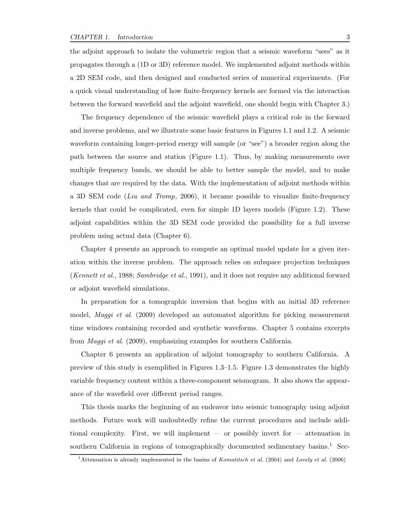
CHAPTER 1. Introduction 3

the adjoint approach to isolate the volumetric region that a seismic waveform “sees” as it

propagates through a (1D or 3D) reference model. We implemented adjoint methods within

a 2D SEM code, and then designed and conducted series of numerical experiments. (For

a quick visual understanding of how finite-frequency kernels are formed via the interaction

between the forward wavefield and the adjoint wavefield, one should begin with Chapter 3.)

The frequency dependence of the seismic wavefield plays a critical role in the forward

and inverse problems, and we illustrate some basic features in Figures 1.1 and 1.2. A seismic

waveform containing longer-period energy will sample (or “see”) a broader region along the

path between the source and station (Figure 1.1). Thus, by making measurements over

multiple frequency bands, we should be able to better sample the model, and to make

changes that are required by the data. With the implementation of adjoint methods within

a 3D SEM code (Liu and Tromp, 2006), it became possible to visualize finite-frequency

kernels that could be complicated, even for simple 1D layers models (Figure 1.2). These

adjoint capabilities within the 3D SEM code provided the possibility for a full inverse

problem using actual data (Chapter 6).

Chapter 4 presents an approach to compute an optimal model update for a given iter-

ation within the inverse problem. The approach relies on subspace projection techniques

(Kennett et al., 1988; Sambridge et al., 1991), and it does not require any additional forward

or adjoint wavefield simulations.

In preparation for a tomographic inversion that begins with an initial 3D reference

model, Maggi et al. (2009) developed an automated algorithm for picking measurement

time windows containing recorded and synthetic waveforms. Chapter 5 contains excerpts

from Maggi et al. (2009), emphasizing examples for southern California.

Chapter 6 presents an application of adjoint tomography to southern California. A

preview of this study is exemplified in Figures 1.3–1.5. Figure 1.3 demonstrates the highly

variable frequency content within a three-component seismogram. It also shows the appear-

ance of the wavefield over different period ranges.

This thesis marks the beginning of an endeavor into seismic tomography using adjoint

methods. Future work will undoubtedly refine the current procedures and include addi-

tional complexity. First, we will implement — or possibly invert for — attenuation in

southern California in regions of tomographically documented sedimentary basins.1 Sec-

1Attenuation is already implemented in the basins of Komatitsch et al. (2004) and Lovely et al. (2006)

CHAPTER 1. Introduction 4

ond, we will consider crustal anisotropy (e.g., Christensen and Mooney , 1995; Paulssen,

2004) and boundary surfaces (e.g., Fuis et al., 2003; Yan and Clayton, 2007; Bleibinhaus

et al., 2007) as inversion parameters. The prospects of inverting for these parameters are

discussed in Sieminski et al. (2007) for anisotropy and in Dahlen (2005) and Tromp et al.

(2005) for boundary surfaces.

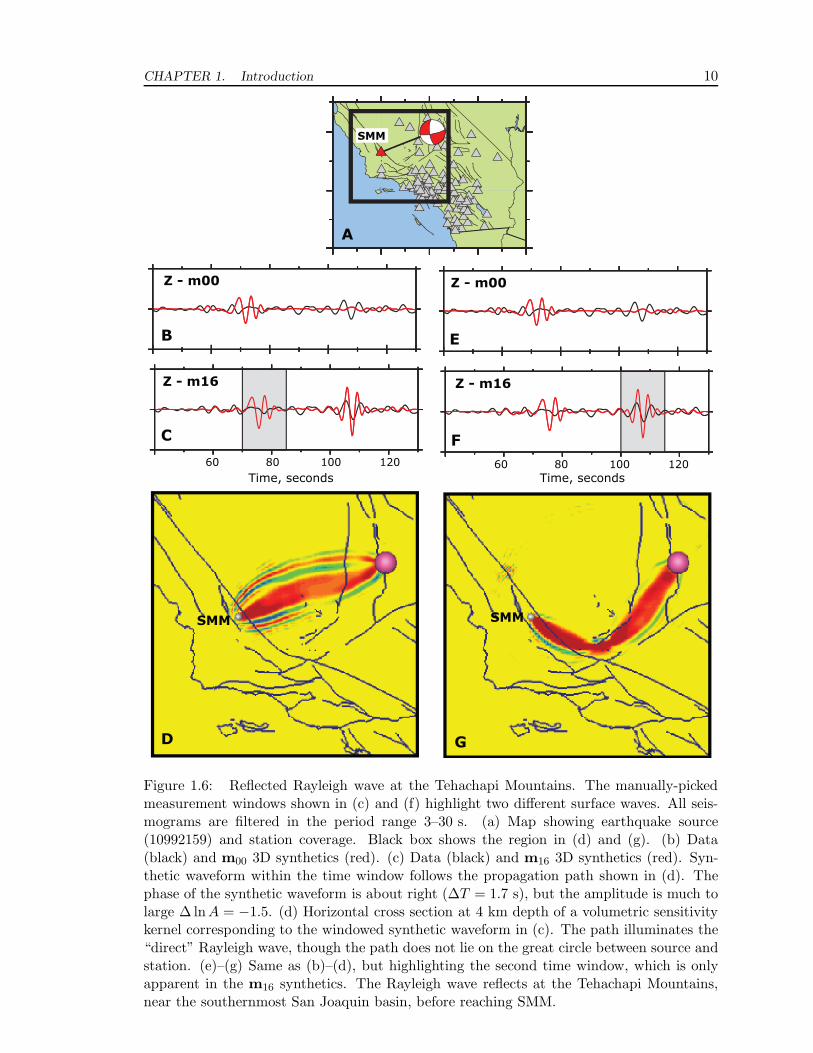
Finally, we will apply seismic reflection imaging techniques (e.g., Kiyashchenko et al.,

2007) to identify and quantify lateral and vertical reflectors in southern California. Fig-

ure 1.6 shows an example of a Rayleigh-wave reflection off of the Tehachapi Mountains.

The reflected waveform is not apparent in the synthetic seismogram from the initial 3D

model (m00) but is in the final model (m16). The ability to capture such waveforms on

individual seismograms demonstrates the possibility of enhancing tomographic coverage by

delving deeper into seismograms while using the same set of earthquakes and stations.

CHAPTER 1. Introduction 5

-1.0

-0.5

0.0

0.5

1.0

Am

plitu

de

0 10 20 30

Time (s)

-1.0

-0.5

0.0

0.5

1.0

Am

plitu

de

0 10 20 30

Time (s)

-1.0

-0.5

0.0

0.5

1.0

Am

plitu

de

0 10 20 30

Time (s)

(a) Regular Source

-2

-1

0

1

2

K_

β (z

)

0 40 80

z (km)

-2

-1

0

1

2

K_

β (z

)

0 40 80

z (km)

(d) Kernel Cross-Sections

-2

-1

0

1

2

0

40

80

z (k

m)

0 50 100 150 200

x (km)

(b) K_β (τ = 8.0 s)

0

40

80

z (k

m)

0 50 100 150 200

x (km)

0

40

80z (k

m)

0 50 100 150 200

x (km)

-2 -1 0 1 2

Traveltime kernel K_β (10 -8 s m -2 )

L

D

(c) K_β (τ = 4.0 s)

0

40

80z (k

m)

0 50 100 150 200

x (km)

Figure 1.1: Frequency dependence of sensitivity kernels (after Tromp et al., 2005, Figure 6).(a) Two source-time functions for the regular wavefield with durations of τ = 8.0 s (gray)and τ = 4.0 s (black) (see Eq. 3.2). (b) K̄β(αρ) for τ = 8.0 s. (c) K̄β(αρ) for τ = 4.0 s.

D = 33 km is the width of the first Fresnel zone, estimated as D ≈√

λL =√

βTL, whereT = 3.4 s is the dominant period of the seismic wave, and β = 3.2 km/s is the shearwavespeed and L = 100 km is the path length. (d) Depth cross sections of (b) and (c) ata horizontal distance of x = 100 km. As expected, the higher-frequency kernel is narrowerin width and greater in amplitude. See Chapter 3 for details on how these kernels wereconstructed.

CHAPTER 1. Introduction 6

R

S

Vertical

Radial

Dis

pla

cem

ent

(10

-4 m

)

10

0

-4

-2

2

2

0

-2

20 30 40 50 60 70

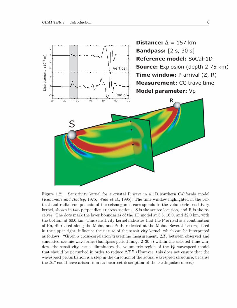
Distance: Δ = 157 km

Bandpass: [2 s, 30 s]

Reference model: SoCal-1D

Source: Explosion (depth 2.75 km)

Time window: P arrival (Z, R)

Measurement: CC traveltime

Model parameter: Vp

Figure 1.2: Sensitivity kernel for a crustal P wave in a 1D southern California model(Kanamori and Hadley , 1975; Wald et al., 1995). The time window highlighted in the ver-tical and radial components of the seismograms corresponds to the volumetric sensitivitykernel, shown in two perpendicular cross sections. S is the source location, and R is the re-ceiver. The dots mark the layer boundaries of the 1D model at 5.5, 16.0, and 32.0 km, withthe bottom at 60.0 km. This sensitivity kernel indicates that the P arrival is a combinationof Pn, diffracted along the Moho, and PmP, reflected at the Moho. Several factors, listedin the upper right, influence the nature of the sensitivity kernel, which can be interpretedas follows: “Given a cross-correlation traveltime measurement, ∆T , between observed andsimulated seismic waveforms (bandpass period range 2–30 s) within the selected time win-dow, the sensitivity kernel illuminates the volumetric region of the VP wavespeed modelthat should be perturbed in order to reduce ∆T .” (However, this does not ensure that thewavespeed perturbation is a step in the direction of the actual wavespeed structure, becausethe ∆T could have arisen from an incorrect description of the earthquake source.)

CHAPTER 1. Introduction 7

−40

−30

−20

−10

0

−100 −50 0 50 100 150 200 250

−40

−30

−20

−10

0

−100 −50 0 50 100 150 200 250

2

3

4

km/s

SA MC

A

Vs m16

20 30 40 50 60 70 80 9020 30 40 50 60 70 80 9020 30 40 50 60 70 80 90

T−m16

R−m16

Z−m16

B

20 30 40 50 60 70 80 9020 30 40 50 60 70 80 9020 30 40 50 60 70 80 90

T−m16

R−m16

Z−m16

C

20 30 40 50 60 70 80 9020 30 40 50 60 70 80 9020 30 40 50 60 70 80 90

T−m16

R−m16

Z−m16

D

Figure 1.3: The frequency dependence of the seismic wavefield. (a) Cross section of adjointtomography crustal model m16 (Chapter 6) from event 14186612 to station FMP.CI. SA, SanAndreas fault; MC, Malibu Coast fault. (b) Data (black) and 3D synthetics (red), filteredin the period range 6–30 s. Z, vertical component, R, radial component, T, transversecomponent. (c) Same as (b), for the period range 3–30 s. (d) Same as (b), for the periodrange 2–30 s.

CHAPTER 1. Introduction 8

40 60 80 100 120 140 16040 60 80 100 120 140 16040 60 80 100 120 140 160

T−m16

R−m16

Z−m16

40 60 80 100 120 140 16040 60 80 100 120 140 16040 60 80 100 120 140 160

T−m00

R−m00

Z−m00

40 60 80 100 120 140 16040 60 80 100 120 140 16040 60 80 100 120 140 160

T−1D

R−1D

Z−1D

B

Figure 1.4: Iterative improvement in seismic waveforms. (a) Initial 3D model m00, final3D model m16, and the difference between the two models, ln(m16/m00). (b) Data (black)and 3D synthetics (red), filtered in the period range 6–30 s. Z, vertical component, R,radial component, T, transverse component. Left column: synthetics generated using thestandard 1D southern California model (Kanamori and Hadley , 1975; Wald et al., 1995).Center column: synthetics generated using m00, the 3D model of Komatitsch et al. (2004).Right column: synthetics generated using m16, the 16th iteration of the crustal model.

CHAPTER 1. Introduction 9

40 60 80 100 120 140 16040 60 80 100 120 140 16040 60 80 100 120 140 160

T−m16

R−m16

Z−m16

40 60 80 100 120 140 16040 60 80 100 120 140 16040 60 80 100 120 140 160

T−m00

R−m00

Z−m00

40 60 80 100 120 140 16040 60 80 100 120 140 16040 60 80 100 120 140 160

T−1D

R−1D

Z−1D

A

40 60 80 100 120 140 16040 60 80 100 120 140 16040 60 80 100 120 140 160

T−m16

R−m16

Z−m16

40 60 80 100 120 140 16040 60 80 100 120 140 16040 60 80 100 120 140 160

T−m00

R−m00

Z−m00

40 60 80 100 120 140 16040 60 80 100 120 140 16040 60 80 100 120 140 160

T−1D

R−1D

Z−1D

B

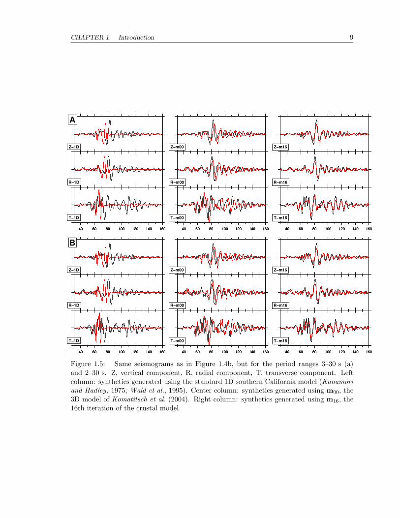
Figure 1.5: Same seismograms as in Figure 1.4b, but for the period ranges 3–30 s (a)and 2–30 s. Z, vertical component, R, radial component, T, transverse component. Leftcolumn: synthetics generated using the standard 1D southern California model (Kanamori

and Hadley , 1975; Wald et al., 1995). Center column: synthetics generated using m00, the3D model of Komatitsch et al. (2004). Right column: synthetics generated using m16, the16th iteration of the crustal model.

CHAPTER 1. Introduction 10

Z - m16 Z - m16

Z - m00Z - m00

SMM

A

B

C

D

E

F

G

8060 100 1208060 100 120

Time, seconds Time, seconds

SMM SMM

Figure 1.6: Reflected Rayleigh wave at the Tehachapi Mountains. The manually-pickedmeasurement windows shown in (c) and (f) highlight two different surface waves. All seis-mograms are filtered in the period range 3–30 s. (a) Map showing earthquake source(10992159) and station coverage. Black box shows the region in (d) and (g). (b) Data(black) and m00 3D synthetics (red). (c) Data (black) and m16 3D synthetics (red). Syn-thetic waveform within the time window follows the propagation path shown in (d). Thephase of the synthetic waveform is about right (∆T = 1.7 s), but the amplitude is much tolarge ∆ lnA = −1.5. (d) Horizontal cross section at 4 km depth of a volumetric sensitivitykernel corresponding to the windowed synthetic waveform in (c). The path illuminates the“direct” Rayleigh wave, though the path does not lie on the great circle between source andstation. (e)–(g) Same as (b)–(d), but highlighting the second time window, which is onlyapparent in the m16 synthetics. The Rayleigh wave reflects at the Tehachapi Mountains,near the southernmost San Joaquin basin, before reaching SMM.