
Intro to Microsoft Access
37
Intro to Microsoft Access Created for DUSPViz by Luke Mich | Fall 2016
-
Upload
duspviz -
Category
Data & Analytics
-
view
104 -
download
0
Transcript of Intro to Microsoft Access

Intro to Microsoft AccessCreated for DUSPViz by Luke Mich | Fall 2016
Intro to Microsoft Access | DUSPViz | Fall 2016 | Page 2
What is Microsoft Access?Access, part of the Microsoft Office Suite, is designed to work with relational databases and is therefore referred to as a database management system (DBMS). Access can be used to create data tables for storing information, queries for parsing subsets of tables, forms for displaying and entering data, and reports for printing and distribution. In this tutorial, we’ll go over some of the basics of relational databases, entering data into Access, and answering questions using queries.
Intro to Microsoft Access | DUSPViz | Fall 2016 | Page 3
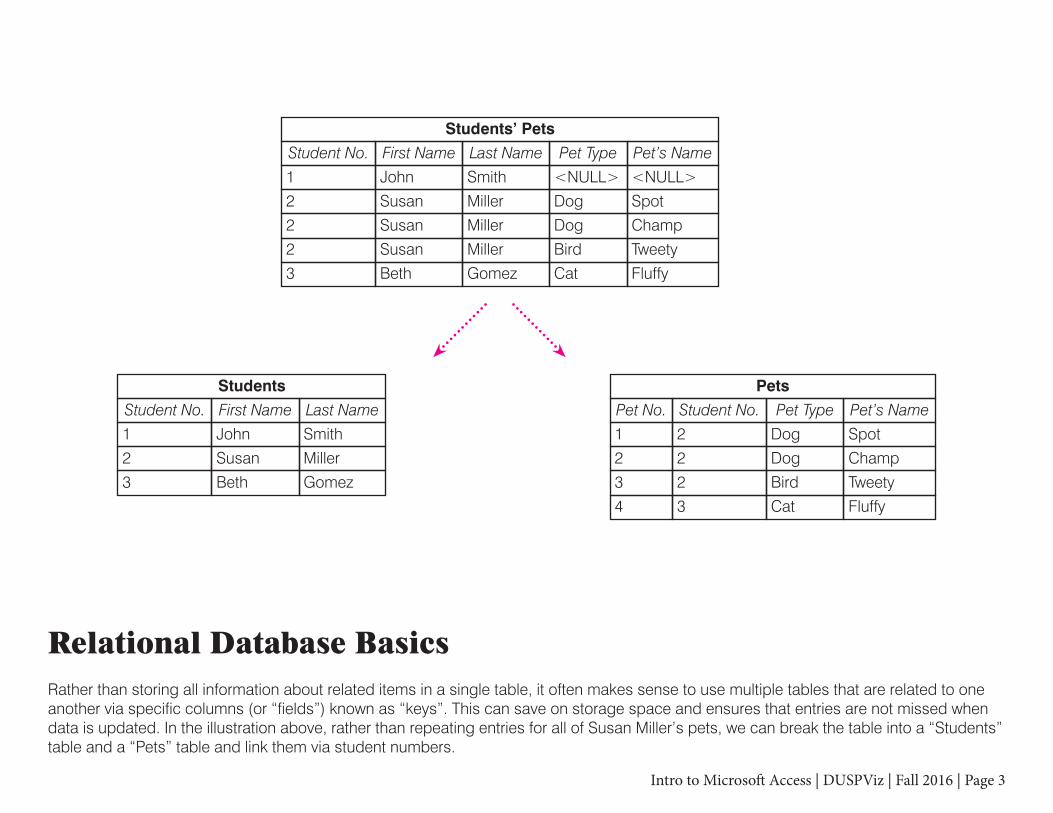
Relational Database BasicsRather than storing all information about related items in a single table, it often makes sense to use multiple tables that are related to one another via specific columns (or “fields”) known as “keys”. This can save on storage space and ensures that entries are not missed when data is updated. In the illustration above, rather than repeating entries for all of Susan Miller’s pets, we can break the table into a “Students” table and a “Pets” table and link them via student numbers.
First Name
Students’ Pets
Student No.
1
2
2
2
3
John
Susan
Susan
Susan
Beth
Last Name
Smith
Miller
Miller
Miller
Gomez
Pet’s Name
<NULL>
Spot
Champ
Tweety
Fluffy
Pet Type
<NULL>
Dog
Dog
Bird
Cat
Student No.
1
2
3
First Name
Students
John
Susan
Beth
Last Name
Smith
Miller
Gomez
Student No.Pet No.
23
22
21
34
Pets
Pet’s Name
Spot
Champ
Tweety
Fluffy
Pet Type
Dog
Dog
Bird
Cat
Intro to Microsoft Access | DUSPViz | Fall 2016 | Page 4
Student No.
1
2
3
First Name
Students
John
Susan
Beth
Last Name
Smith
Miller
Gomez
Student No.Pet No.
23
22
21
34
Pets
Pet’s Name
Spot
Champ
Tweety
Fluffy
Pet Type
Dog
Dog
Bird
Cat
PrimaryKey
PrimaryKey
ForeignKey
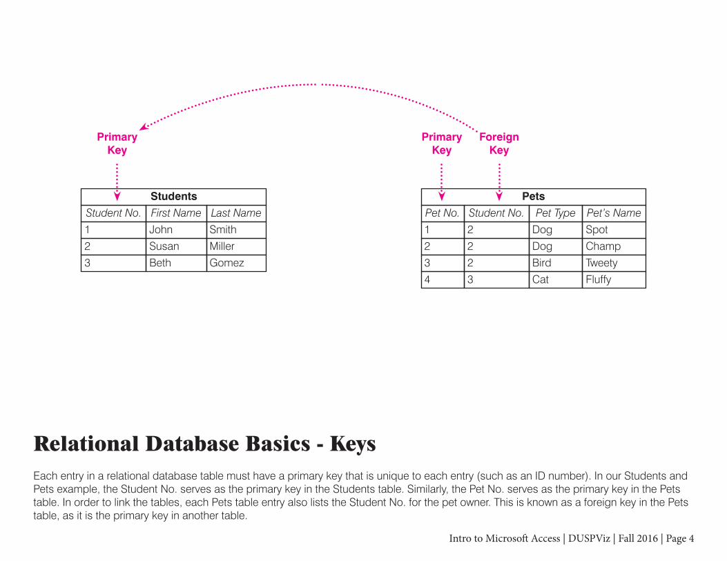
Relational Database Basics - KeysEach entry in a relational database table must have a primary key that is unique to each entry (such as an ID number). In our Students and Pets example, the Student No. serves as the primary key in the Students table. Similarly, the Pet No. serves as the primary key in the Pets table. In order to link the tables, each Pets table entry also lists the Student No. for the pet owner. This is known as a foreign key in the Pets table, as it is the primary key in another table.

Intro to Microsoft Access | DUSPViz | Fall 2016 | Page 5
Relational Database Basics - Relationship TypesIn the previous example, we had a one-to-many relationship as each student can have many pets. Other relationship types include one-to-one and many-to-many. One-to-one relationships, while uncommon, can be used to store infrequently used data in another table (e.g. a table of products may include basic descriptions while a second table may contain more technical specifications for each product that can be joined to the first table on a one-to-one basis when needed. The many-to-many relationship, considered the most complex, is illustrated in the above example. Each student in the Students table can take many courses in the Courses table and each course can be taken by many students. In cases such as these, a third table, known as a match, junction, or mapping table is needed to connect the other two tables. For us, the Enrollment table contains a unique entry for each enrollment pairing of a student and course. The Enrollment table, and all match tables, must contain foreign keys that can be matched to the primary keys of the tables that require matching.
Student No.
1
2
3
First Name
Students
John
Susan
Beth
Last Name
Smith
Miller
Gomez
Course No. Student No.EID
2
4
1
2
3
7
1
3
3
2
2
6
1 11
2
4
2
2
3
3
4
8
5
Enrollment
Course No.
3
2
1
4
Courses
Course
Math
English
Science
Gym
PrimaryKey
PrimaryKey
PrimaryKey
ForeignKey
ForeignKey

Intro to Microsoft Access | DUSPViz | Fall 2016 | Page 6
Opening AccessNow that we’ve got a basic understanding of relational databases, let’s start the tutorial. When you open Access, you’ll be prompted to select a template type. the default choices include commonly used form and table types as well as web-based database options. Let’s select the “Blank Desktop Database” option. You’ll be prompted to name and save the file.
Intro to Microsoft Access | DUSPViz | Fall 2016 | Page 7
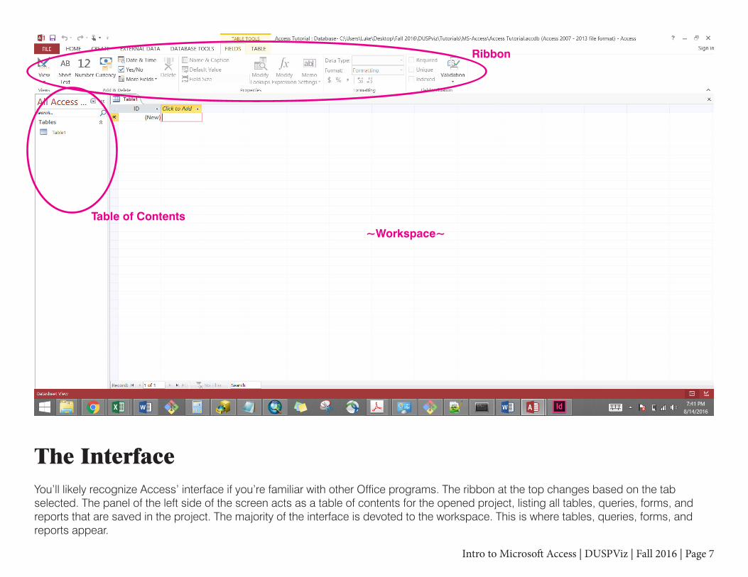
The InterfaceYou’ll likely recognize Access’ interface if you’re familiar with other Office programs. The ribbon at the top changes based on the tab selected. The panel of the left side of the screen acts as a table of contents for the opened project, listing all tables, queries, forms, and reports that are saved in the project. The majority of the interface is devoted to the workspace. This is where tables, queries, forms, and reports appear.
Ribbon
Table of Contents
~Workspace~

Intro to Microsoft Access | DUSPViz | Fall 2016 | Page 8
Importing DataWe’ll begin by importing some existing data - a CSV of Massachusetts’ counties and their FIPS codes, a CSV of Massachusetts’ census tracts and their areas, and an Excel file of ACS income data for Massachusetts’ census tracts. Go to the Home tab and select Text File from the “Import & Link” panel. Navigate to the folder in which you’ve saved the tutorial materials and select “CountyFIPS.csv.” Select Import the source data into a new table in the current database and click OK.
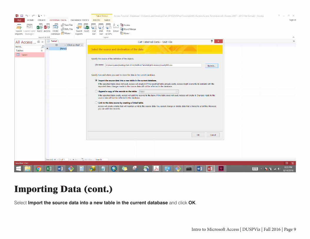
Intro to Microsoft Access | DUSPViz | Fall 2016 | Page 9
Importing Data (cont.)Select Import the source data into a new table in the current database and click OK.

Intro to Microsoft Access | DUSPViz | Fall 2016 | Page 10
Importing Data (cont.)Select Delimited and click Next.
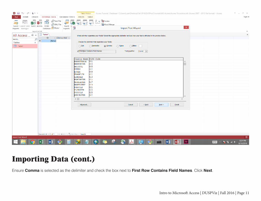
Intro to Microsoft Access | DUSPViz | Fall 2016 | Page 11
Importing Data (cont.)Ensure Comma is selected as the delimiter and check the box next to First Row Contains Field Names. Click Next.
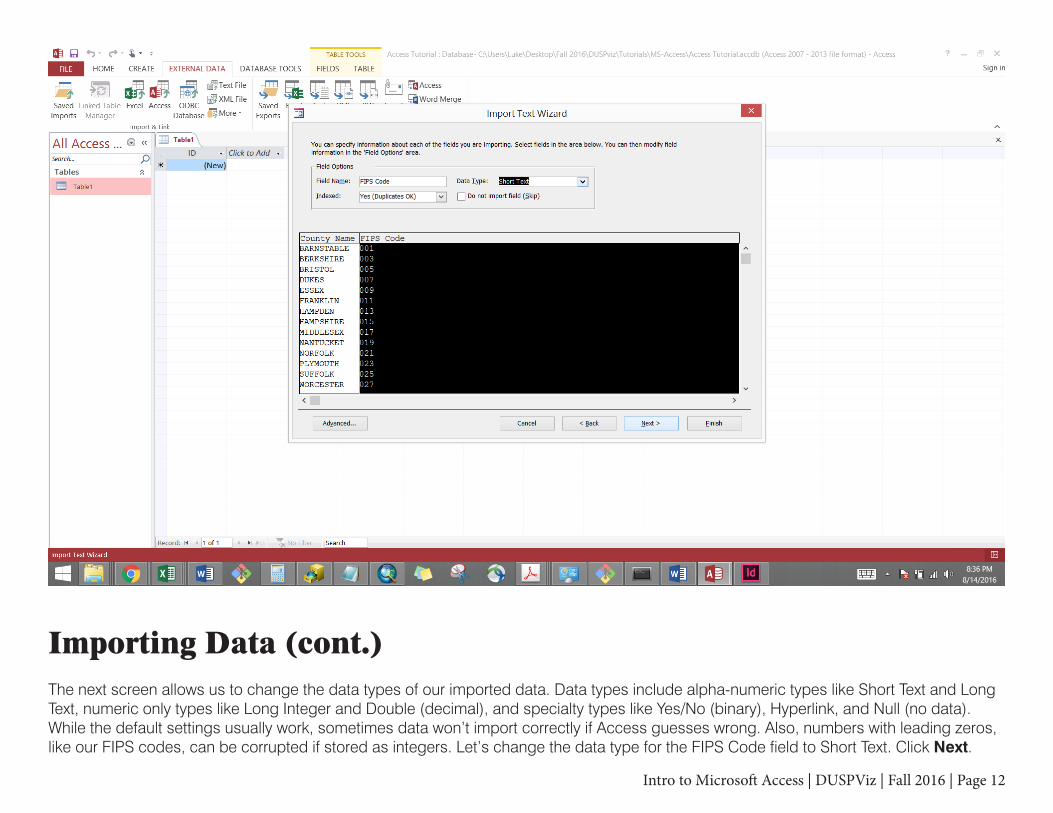
Intro to Microsoft Access | DUSPViz | Fall 2016 | Page 12
Importing Data (cont.)The next screen allows us to change the data types of our imported data. Data types include alpha-numeric types like Short Text and Long Text, numeric only types like Long Integer and Double (decimal), and specialty types like Yes/No (binary), Hyperlink, and Null (no data). While the default settings usually work, sometimes data won’t import correctly if Access guesses wrong. Also, numbers with leading zeros, like our FIPS codes, can be corrupted if stored as integers. Let’s change the data type for the FIPS Code field to Short Text. Click Next.

Intro to Microsoft Access | DUSPViz | Fall 2016 | Page 13
Importing Data (cont.)Access can create a new field containing sequential integers as primary keys. However, since we will eventually link this data to our other tables, we should select a field that uniquely identifies each entry that will also be listed in at least one of our other tables. Let’s select the button next to Choose my own primary key and use the drop down menu to select the FIPS Code field. Click Next.
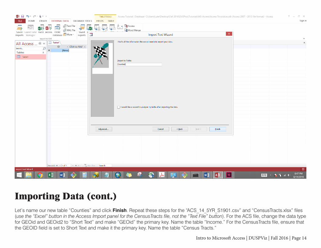
Intro to Microsoft Access | DUSPViz | Fall 2016 | Page 14
Importing Data (cont.)Let’s name our new table “Counties” and click Finish. Repeat these steps for the “ACS_14_5YR_S1901.csv” and “CensusTracts.xlsx” files (use the “Excel” button in the Access Import panel for the CensusTracts file, not the “Text File” button). For the ACS file, change the data type for GEOid and GEOid2 to “Short Text” and make “GEOid” the primary key. Name the table “Income.” For the CensusTracts file, ensure that the GEOID field is set to Short Text and make it the primary key. Name the table “Census Tracts.”
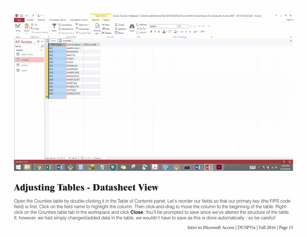
Intro to Microsoft Access | DUSPViz | Fall 2016 | Page 15
Adjusting Tables - Datasheet ViewOpen the Counties table by double-clicking it in the Table of Contents panel. Let’s reorder our fields so that our primary key (the FIPS code field) is first. Click on the field name to highlight the column. Then click-and-drag to move the column to the beginning of the table. Right-click on the Counties table tab in the workspace and click Close. You’ll be prompted to save since we’ve altered the structure of the table. If, however, we had simply changed/added data in the table, we wouldn’t have to save as this is done automatically - so be careful!
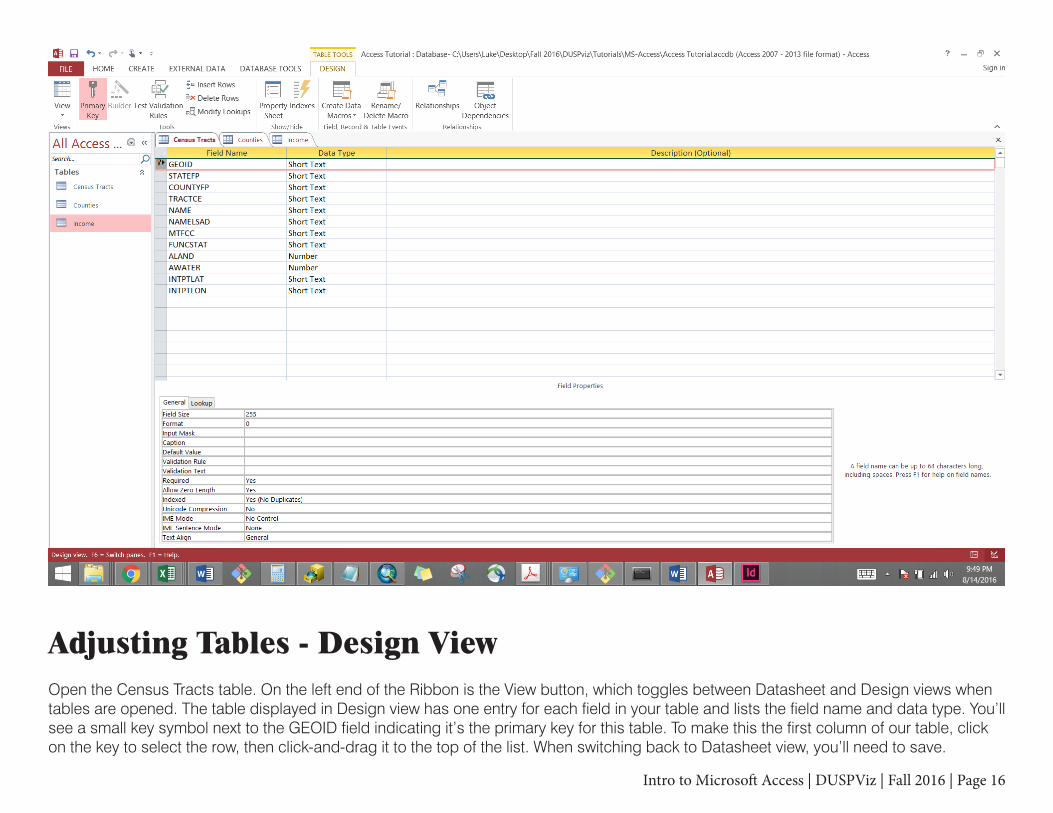
Intro to Microsoft Access | DUSPViz | Fall 2016 | Page 16
Adjusting Tables - Design ViewOpen the Census Tracts table. On the left end of the Ribbon is the View button, which toggles between Datasheet and Design views when tables are opened. The table displayed in Design view has one entry for each field in your table and lists the field name and data type. You’ll see a small key symbol next to the GEOID field indicating it’s the primary key for this table. To make this the first column of our table, click on the key to select the row, then click-and-drag it to the top of the list. When switching back to Datasheet view, you’ll need to save.
Intro to Microsoft Access | DUSPViz | Fall 2016 | Page 17
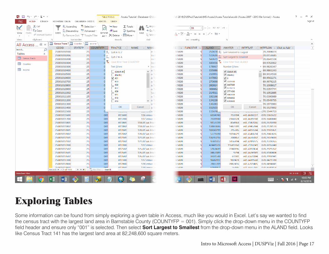
Exploring TablesSome information can be found from simply exploring a given table in Access, much like you would in Excel. Let’s say we wanted to find the census tract with the largest land area in Barnstable County (COUNTYFP = 001). Simply click the drop-down menu in the COUNTYFP field header and ensure only “001” is selected. Then select Sort Largest to Smallest from the drop-down menu in the ALAND field. Looks like Census Tract 141 has the largest land area at 82,248,600 square meters.
Intro to Microsoft Access | DUSPViz | Fall 2016 | Page 18
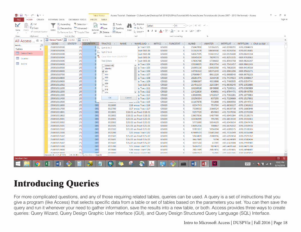
Introducing QueriesFor more complicated questions, and any of those requiring related tables, queries can be used. A query is a set of instructions that you give a program (like Access) that selects specific data from a table or set of tables based on the parameters you set. You can then save the query and run it whenever your need to gather information, save the results into a new table, or both. Access provides three ways to create queries: Query Wizard, Query Design Graphic User Interface (GUI), and Query Design Structured Query Language (SQL) Interface.
Intro to Microsoft Access | DUSPViz | Fall 2016 | Page 19
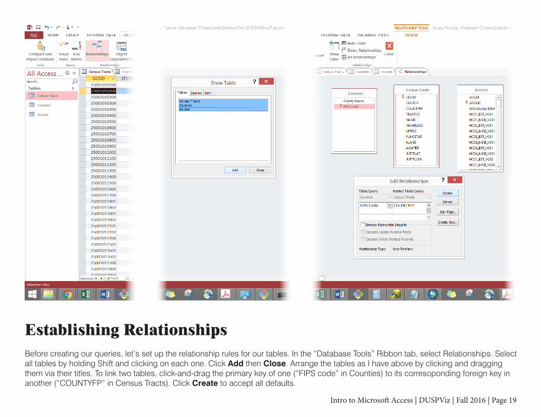
Establishing RelationshipsBefore creating our queries, let’s set up the relationship rules for our tables. In the “Database Tools” Ribbon tab, select Relationships. Select all tables by holding Shift and clicking on each one. Click Add then Close. Arrange the tables as I have above by clicking and dragging them via their titles. To link two tables, click-and-drag the primary key of one (“FIPS code” in Counties) to its corresoponding foreign key in another (“COUNTYFP” in Census Tracts). Click Create to accept all defaults.
Intro to Microsoft Access | DUSPViz | Fall 2016 | Page 20
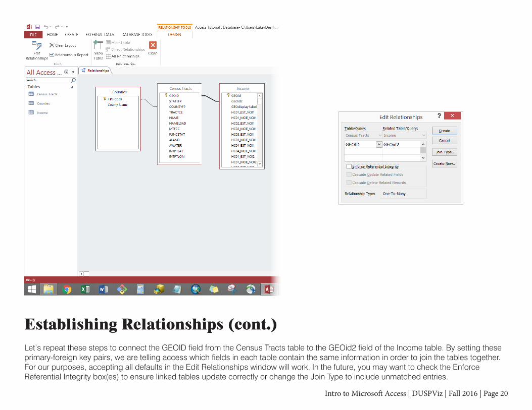
Establishing Relationships (cont.)Let’s repeat these steps to connect the GEOID field from the Census Tracts table to the GEOid2 field of the Income table. By setting these primary-foreign key pairs, we are telling access which fields in each table contain the same information in order to join the tables together. For our purposes, accepting all defaults in the Edit Relationships window will work. In the future, you may want to check the Enforce Referential Integrity box(es) to ensure linked tables update correctly or change the Join Type to include unmatched entries.

Intro to Microsoft Access | DUSPViz | Fall 2016 | Page 21
Query WizardThe simplest query creation method is the Query Wizard. From the Create Ribbon, click the Query Wizard button. (1) Select Simple Query Wizard and click OK. We’d like to see the total number of households (fields for the Income table are defined in the ACS_14_5YR_S1901_metadata.csv file) and the land area for each census tract. (2) Select the Income table from the dropdown menu and double-click the GEOdisplay-label and HC01_EST_VC01 fields to move them to the “Selected Fields” area. (3) Now select the Census Tracts table from the drop-down and double-click the ALAND field to add it to our query; click Next. (4) Check the Detail button to list all entries, and click Next. (5) Name our query “Households and Land Area,” and click Finish.
(1)
(2)
(4)
(3)
(5)
Intro to Microsoft Access | DUSPViz | Fall 2016 | Page 22
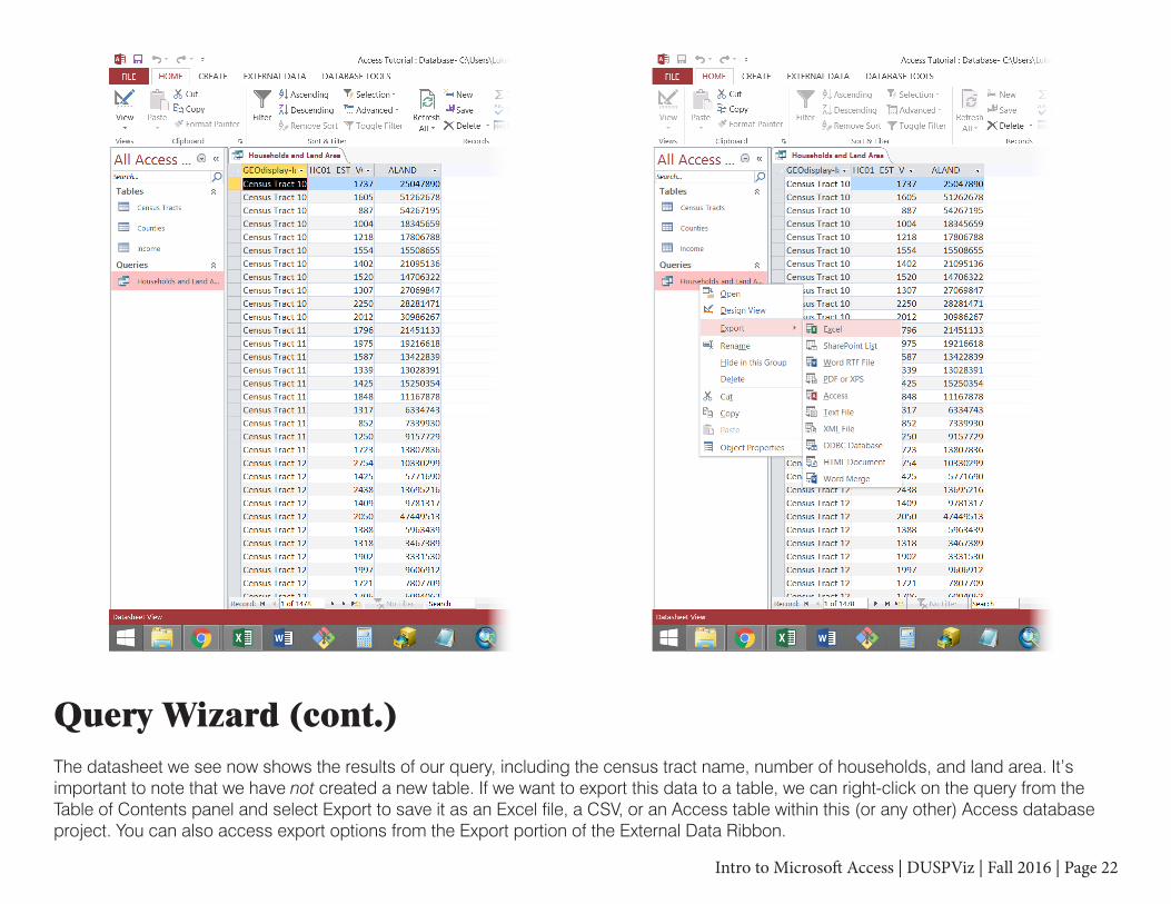
Query Wizard (cont.)The datasheet we see now shows the results of our query, including the census tract name, number of households, and land area. It’s important to note that we have not created a new table. If we want to export this data to a table, we can right-click on the query from the Table of Contents panel and select Export to save it as an Excel file, a CSV, or an Access table within this (or any other) Access database project. You can also access export options from the Export portion of the External Data Ribbon.
Intro to Microsoft Access | DUSPViz | Fall 2016 | Page 23
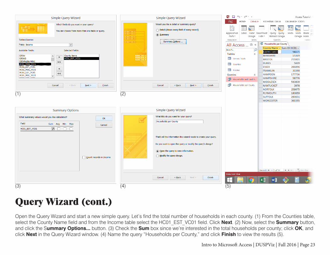
Query Wizard (cont.)Open the Query Wizard and start a new simple query. Let’s find the total number of households in each county. (1) From the Counties table, select the County Name field and from the Income table select the HC01_EST_VC01 field. Click Next. (2) Now, select the Summary button, and click the Summary Options... button. (3) Check the Sum box since we’re interested in the total households per county; click OK, and click Next in the Query Wizard window. (4) Name the query “Households per County,” and click Finish to view the results (5).
(1)
(3)
(2)
(4) (5)

Intro to Microsoft Access | DUSPViz | Fall 2016 | Page 24
Query Design GUIFor more complicated queries, we can use the Query Design Graphic User Interface, or GUI (pronounce “gooey”). This lets us customize more parts of our queries. Open the Query Design GUI by clicking Query Design from the Create Ribbon. Select all tables, click Add, and then click Close. Once the tables are loaded, you can rearrange them by clicking and dragging on their title bars and resizing them by clicking and dragging their corners. You’ll see the relationship links that we previously set up appear.
Intro to Microsoft Access | DUSPViz | Fall 2016 | Page 25
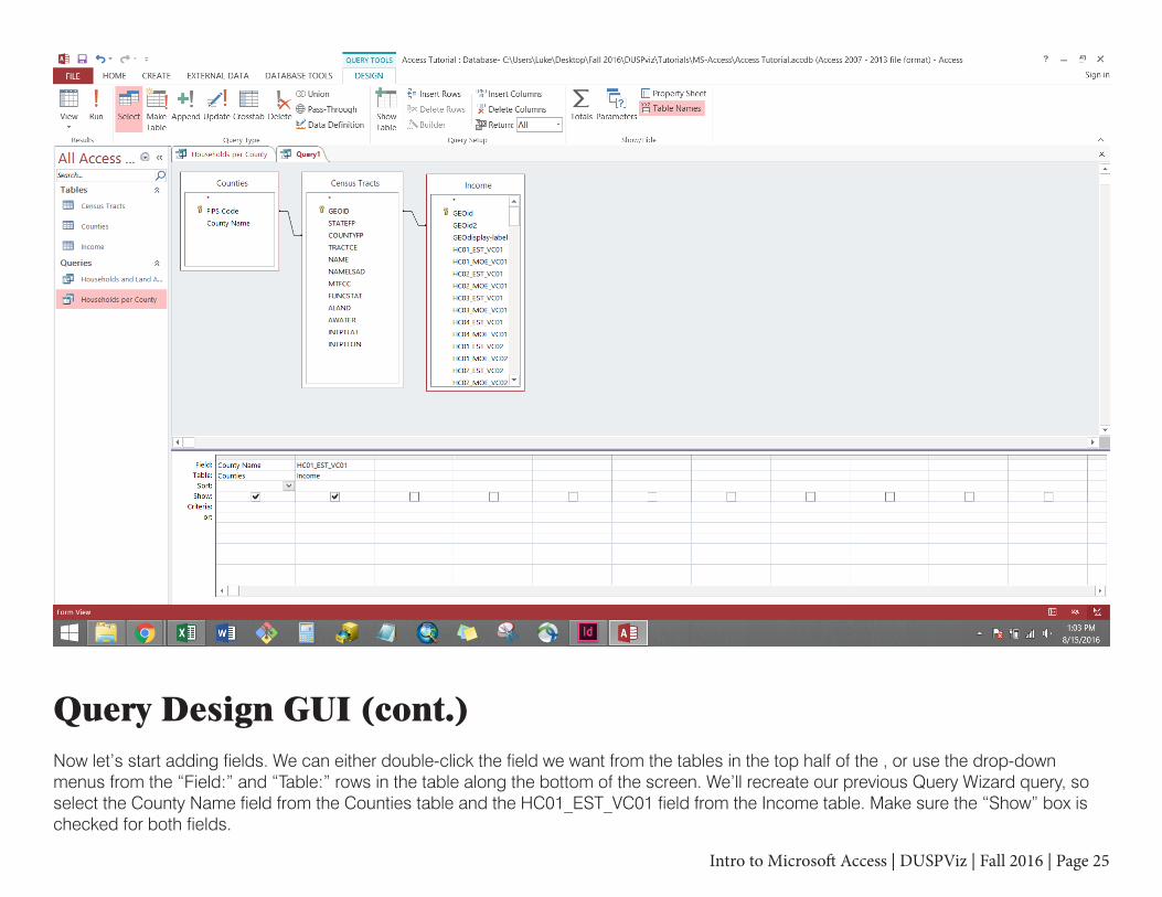
Query Design GUI (cont.)Now let’s start adding fields. We can either double-click the field we want from the tables in the top half of the , or use the drop-down menus from the “Field:” and “Table:” rows in the table along the bottom of the screen. We’ll recreate our previous Query Wizard query, so select the County Name field from the Counties table and the HC01_EST_VC01 field from the Income table. Make sure the “Show” box is checked for both fields.

Intro to Microsoft Access | DUSPViz | Fall 2016 | Page 26
Query Design GUI (cont.)If we ran this query now, we would have one row per entry in the income table, since we have not told Access to group or summarize our data. Right click in any cell in the Query Design info table and click Totals. Leave “Group By” in the County Name Totals cell, but change the Totals to “Sum” for HC01_EST_VC01 using the drop-down menu. This will group the census tract household counts by county and sum that information. Click Datasheet View or Run to view the results. It should be the same as the previous Query Wizard query.
Intro to Microsoft Access | DUSPViz | Fall 2016 | Page 27
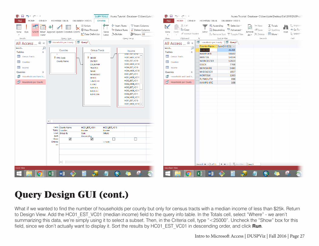
Query Design GUI (cont.)What if we wanted to find the number of households per county but only for census tracts with a median income of less than $25k. Return to Design View. Add the HC01_EST_VC01 (median income) field to the query info table. In the Totals cell, select “Where” - we aren’t summarizing this data, we’re simply using it to select a subset. Then, in the Criteria cell, type “<25000”. Uncheck the “Show” box for this field, since we don’t actually want to display it. Sort the results by HC01_EST_VC01 in descending order, and click Run.

Intro to Microsoft Access | DUSPViz | Fall 2016 | Page 28
Query Design GUI (cont.)Instead of a total household count, what if we wanted to know the household density (per sq. mi.) for each county? Let’s delete the HC01_EST_VC13 field from our info table. Right-click in the HC01_EST_VC01 field and click Build... to open the Expression Builder. Copy in the expression shown above. You can add fields by manually typing them or navigating through the Expression Elements/Categories windows. Click OK in the Expression Builder and save our query as County Household Density.
* Note the construction of our expression: we sum the number of households in each census tract and divide by the sum of the land area of each tract. We then multiply by 2589988 to convert from square meters (the unit for “ALAND”) to square miles. We don’t need to account for aggregating by county in this expression because our “Group By” parameter for the County Name field does this for us. We’ve named this caclulated field “HH_Density” by changing the default “Expr_1.”

Intro to Microsoft Access | DUSPViz | Fall 2016 | Page 29
Query SQL InterfaceThe final method of creating queries is the Structured Query Language (SQL) method. Essentially, this is standardized coding that selects a specific subset of data. Open the County Households Density query and switch the view to “SQL View” using the view toggle in the ribbon. This allows you to see what our GUI-built (or Query Wizard-built) queries get translated into so that Access can select our requested data. By learning SQL, you can further customize your queries.

Intro to Microsoft Access | DUSPViz | Fall 2016 | Page 30
SQL BasicsLet’s look more closely at this SQL code. We start with a “SELECT” statement, which tells Access which fields we’re interested in reviewing. Fields are formated as “table.field” (the brackets [] are Access’ way of holding together field and table names that contain spaces). Additionally, we see that our calculated field has been named using the “AS” statement. We can use AS to rename any field, not just calculated ones.

Intro to Microsoft Access | DUSPViz | Fall 2016 | Page 31
SQL Basics (cont.)Next is the “FROM” statement. This selects the tables we’re pulling from. It also lists how our tables are joined together. We see that our Counties table is joined to our Census Tracts table through an “INNER JOIN” on the FIPS Code and COUNTYFP fields and it is joined to our Income table through an “INNER JOIN” on the GEOID and GEOid2 fields. An inner join means that only records with matches in both tables appear (an outer join includes all records, even when they don’t exist in both tables).
Intro to Microsoft Access | DUSPViz | Fall 2016 | Page 32
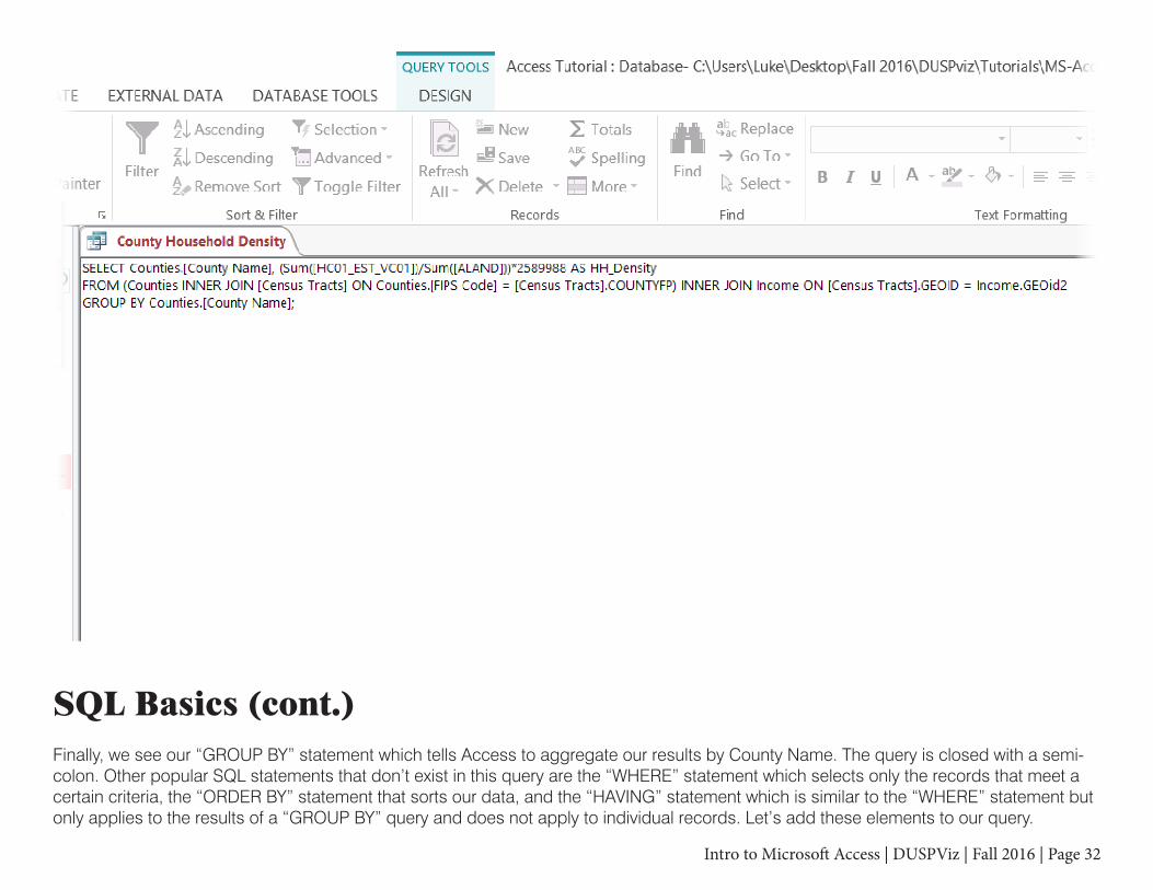
SQL Basics (cont.)Finally, we see our “GROUP BY” statement which tells Access to aggregate our results by County Name. The query is closed with a semi-colon. Other popular SQL statements that don’t exist in this query are the “WHERE” statement which selects only the records that meet a certain criteria, the “ORDER BY” statement that sorts our data, and the “HAVING” statement which is similar to the “WHERE” statement but only applies to the results of a “GROUP BY” query and does not apply to individual records. Let’s add these elements to our query.
Intro to Microsoft Access | DUSPViz | Fall 2016 | Page 33
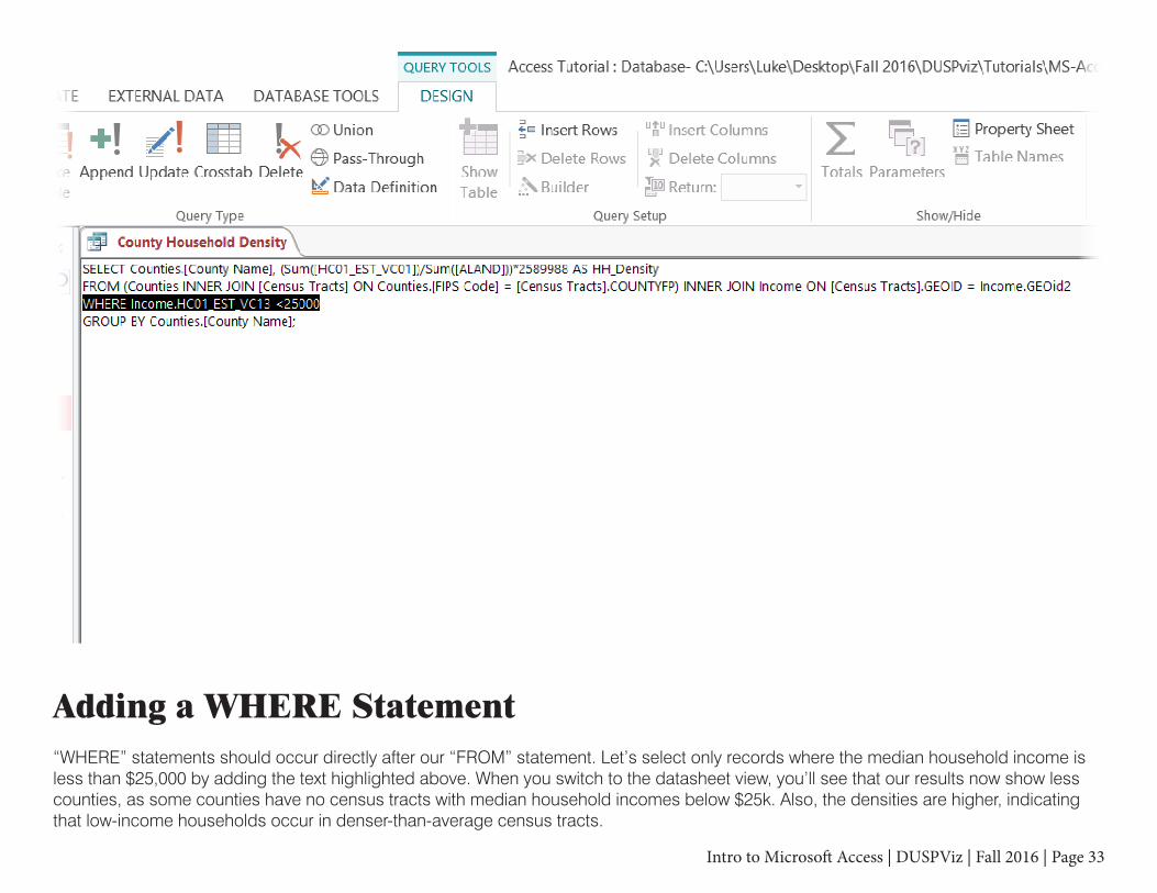
Adding a WHERE Statement“WHERE” statements should occur directly after our “FROM” statement. Let’s select only records where the median household income is less than $25,000 by adding the text highlighted above. When you switch to the datasheet view, you’ll see that our results now show less counties, as some counties have no census tracts with median household incomes below $25k. Also, the densities are higher, indicating that low-income households occur in denser-than-average census tracts.
Intro to Microsoft Access | DUSPViz | Fall 2016 | Page 34
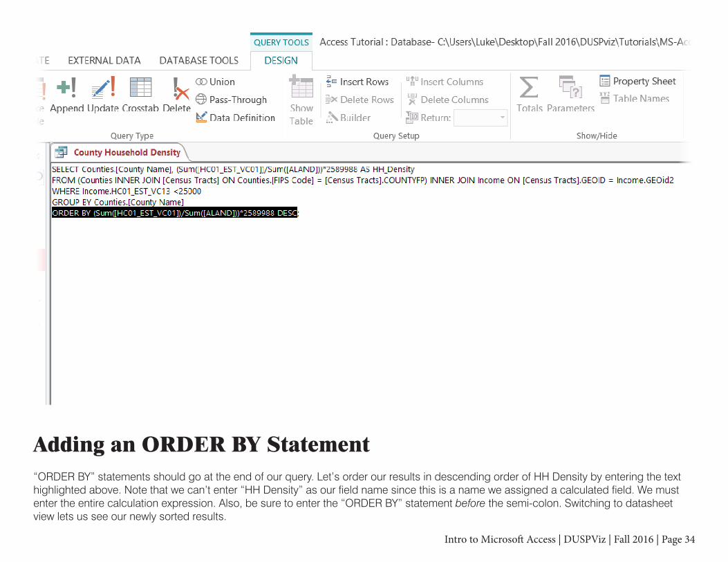
Adding an ORDER BY Statement“ORDER BY” statements should go at the end of our query. Let’s order our results in descending order of HH Density by entering the text highlighted above. Note that we can’t enter “HH Density” as our field name since this is a name we assigned a calculated field. We must enter the entire calculation expression. Also, be sure to enter the “ORDER BY” statement before the semi-colon. Switching to datasheet view lets us see our newly sorted results.
Intro to Microsoft Access | DUSPViz | Fall 2016 | Page 35
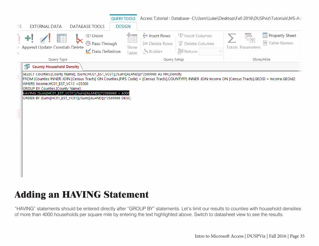
Adding an HAVING Statement“HAVING” statements should be entered directly after “GROUP BY” statements. Let’s limit our results to counties with household densities of more than 4000 households per square mile by entering the text highlighted above. Switch to datasheet view to see the results.
Intro to Microsoft Access | DUSPViz | Fall 2016 | Page 36
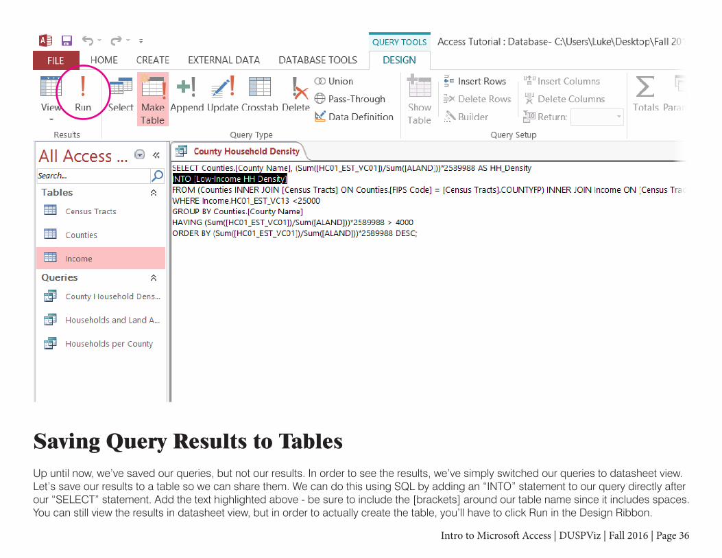
Saving Query Results to TablesUp until now, we’ve saved our queries, but not our results. In order to see the results, we’ve simply switched our queries to datasheet view. Let’s save our results to a table so we can share them. We can do this using SQL by adding an “INTO” statement to our query directly after our “SELECT” statement. Add the text highlighted above - be sure to include the [brackets] around our table name since it includes spaces. You can still view the results in datasheet view, but in order to actually create the table, you’ll have to click Run in the Design Ribbon.
Intro to Microsoft Access | DUSPViz | Fall 2016 | Page 37
Additional ResourcesCheck out lynda.com for additional and advanced MS-Access tutorials. You can also go to the MSDN Access SQL reference site for Access-specific SQL help or W3 Schools for more generic SQL help and basics.


![เรียน-เล่น-เป็นง่าย Access 2007 · Microsoft Access Microsoft Office Professional Access "adî... Access Access Access "îl]î" muùouañoo:ls Access](https://static.fdocuments.net/doc/165x107/5f5793511c90a77e406f5980/aaaaa-aaaa-aaaaaaaa-access-2007-microsoft-access.jpg)


