Interruptions: Using Activity Transitions to Trigger Proactive
116
Interruptions: Using Activity Transitions to Trigger Proactive Messages by Joyce Ho Submitted to the Department of Electrical Engineering and Computer Science in partial fulfillment of the requirements for the degree of Masters of Engineering at the MASSACHUSETTS INSTITUTE OF TECHNOLOGY August 2004 c Massachusetts Institute of Technology 2004. All rights reserved. Author .............................................................. Department of Electrical Engineering and Computer Science August 17, 2004 Certified by .......................................................... Stephen Intille Research Scientist Thesis Supervisor Accepted by ......................................................... Arthur C. Smith Chairman, Department Committee on Graduate Students
Transcript of Interruptions: Using Activity Transitions to Trigger Proactive

Interruptions: Using Activity Transitions to
Trigger Proactive Messages
by
Joyce Ho
Submitted to the Department of Electrical Engineering andComputer Science
in partial fulfillment of the requirements for the degree of
Masters of Engineering
at the
MASSACHUSETTS INSTITUTE OF TECHNOLOGY
August 2004
c© Massachusetts Institute of Technology 2004. All rights reserved.
Author . . . . . . . . . . . . . . . . . . . . . . . . . . . . . . . . . . . . . . . . . . . . . . . . . . . . . . . . . . . . . .Department of Electrical Engineering and Computer Science
August 17, 2004
Certified by. . . . . . . . . . . . . . . . . . . . . . . . . . . . . . . . . . . . . . . . . . . . . . . . . . . . . . . . . .Stephen Intille
Research ScientistThesis Supervisor
Accepted by . . . . . . . . . . . . . . . . . . . . . . . . . . . . . . . . . . . . . . . . . . . . . . . . . . . . . . . . .Arthur C. Smith
Chairman, Department Committee on Graduate Students

2
Interruptions: Using Activity Transitions to Trigger
Proactive Messages
by
Joyce Ho
Submitted to the Department of Electrical Engineering and Computer Scienceon August 17, 2004, in partial fulfillment of the
requirements for the degree ofMasters of Engineering
Abstract
The proliferation of mobile devices and their tendency to present information proac-tively has led to an increase in device generated interruptions experienced by users.These interruptions are not confined to a particular physical space and are om-nipresent. One possible strategy to lower the perceived burden of these interruptionsis to cluster non-time-sensitive interruptions and deliver them during a physical activ-ity transition. Since a user is already “interrupting” the current activity to engage ina new activity, the user will be more receptive to an interruption at this moment. Thiswork compares the user’s receptivity to an interruption triggered by an activity tran-sition against a randomly generated interruption. A mobile computer system detectsan activity transition with the use of wireless accelerometers. The results demonstratethat using this strategy reduces the perceived burden of the interruption.
Thesis Supervisor: Stephen IntilleTitle: Research Scientist
3

4

Acknowledgments
I would like to thank the subjects who participated in the interruption study and
the subjects who helped train and verify the activity transition detection algorithm.
Without their participation, this work would not have been possible.
I would also like to thank the following people:
My advisor, Stephen Intille, for the opportunity to work on this project and his
guidance and support throughout the project.
Emmanuel Mungia Tapia for developing the wireless accelerometers (MITes), help-
ing with the design of the receiver casing, and helping port the wireless receiver code
onto the iPAQ.
Jennifer Beaudin for the design of the sensor encasements, the labels, and the help
in determining the experiment protocol.
T.J. McLeish for his design of the housing for the connectors and making it possible
for users to carry around the wireless receiver without a bulky attachment.
All the House ners for their willingness to be guinea pigs, their feedback, and their
help.
My friends and family for their endless support.
Finally I would like to thank the NSF for supporting this work via ITR award
#0313065.
5

6

Contents
1 Introduction 15
2 Related Work 17
2.1 Defining Interruption . . . . . . . . . . . . . . . . . . . . . . . . . . . 17
2.2 Modeling Interruption . . . . . . . . . . . . . . . . . . . . . . . . . . 19
2.3 Detecting Interruptability with Sensors . . . . . . . . . . . . . . . . . 19
2.4 Detecting Interruptability in Mobile Applications . . . . . . . . . . . 22
3 Experimental Framework 25
3.1 Design and Materials . . . . . . . . . . . . . . . . . . . . . . . . . . . 27
3.2 Procedure . . . . . . . . . . . . . . . . . . . . . . . . . . . . . . . . . 30
3.3 Subjects . . . . . . . . . . . . . . . . . . . . . . . . . . . . . . . . . . 31
4 Results 33
4.1 Verification of Transition Detection Algorithm . . . . . . . . . . . . . 33
4.2 Interruption Study . . . . . . . . . . . . . . . . . . . . . . . . . . . . 37
5 Discussion and Future Work 41
6 Conclusion 47
A Prior Work and Additional Details 49
A.1 Activity of the User . . . . . . . . . . . . . . . . . . . . . . . . . . . . 49
A.2 Utility of Message . . . . . . . . . . . . . . . . . . . . . . . . . . . . . 50
A.3 Emotional State of the User . . . . . . . . . . . . . . . . . . . . . . . 50
7

A.4 Modality of the Interruption . . . . . . . . . . . . . . . . . . . . . . . 51
A.5 Frequency of Interruptions . . . . . . . . . . . . . . . . . . . . . . . . 51
A.6 Comprehension Rate and Expected Length of the Interruption . . . . 52
A.7 Authority Level . . . . . . . . . . . . . . . . . . . . . . . . . . . . . . 52
A.8 Previous and Future Activities of the User . . . . . . . . . . . . . . . 53
A.9 Social Engagement of the User . . . . . . . . . . . . . . . . . . . . . . 53
A.10 Social Expectation of Group Behavior Concerning the User’s Behavior 54
A.11 History of User Interaction and Likelihood of Response . . . . . . . . 54
B Subject Protocol 57
B.1 Recruitment . . . . . . . . . . . . . . . . . . . . . . . . . . . . . . . . 57
B.2 Subject Preparation . . . . . . . . . . . . . . . . . . . . . . . . . . . 58
B.3 Wrap-up Interview . . . . . . . . . . . . . . . . . . . . . . . . . . . . 59
B.4 Accelerometer Placement . . . . . . . . . . . . . . . . . . . . . . . . . 63
C Sample Data Set 65
D Additional Result Details 71
D.1 Verification of Activity Transitions . . . . . . . . . . . . . . . . . . . 71
D.2 Experiment Study Results . . . . . . . . . . . . . . . . . . . . . . . . 74
E Receiver Casing 79
E.1 Parts . . . . . . . . . . . . . . . . . . . . . . . . . . . . . . . . . . . . 79
E.2 Pin-out Diagrams . . . . . . . . . . . . . . . . . . . . . . . . . . . . . 80
E.3 Instructions . . . . . . . . . . . . . . . . . . . . . . . . . . . . . . . . 82
E.3.1 Discharging and Charging the Batteries . . . . . . . . . . . . . 82
E.3.2 Connector Cable . . . . . . . . . . . . . . . . . . . . . . . . . 82
E.3.3 Building the Sleeve Cover . . . . . . . . . . . . . . . . . . . . 83
E.3.4 Preparing the Sleeve Jacket for the Connector . . . . . . . . . 84
E.3.5 Connector Housing . . . . . . . . . . . . . . . . . . . . . . . . 86
E.3.6 Wiring the Connectors . . . . . . . . . . . . . . . . . . . . . . 86
8

F Experiment Graphical User Interface Screenshots 91
F.1 Screen Flow . . . . . . . . . . . . . . . . . . . . . . . . . . . . . . . . 91
F.2 Screen Interface . . . . . . . . . . . . . . . . . . . . . . . . . . . . . . 92
G Feature Calculation and Decision Tree Algorithm 95
G.1 Feature Calculation . . . . . . . . . . . . . . . . . . . . . . . . . . . . 95
G.2 Decision Tree Algorithm . . . . . . . . . . . . . . . . . . . . . . . . . 97
H Training a Classifier 101
H.1 Sampling Window . . . . . . . . . . . . . . . . . . . . . . . . . . . . . 101
H.2 Number of Accelerometers . . . . . . . . . . . . . . . . . . . . . . . . 102
H.3 Type of Activities . . . . . . . . . . . . . . . . . . . . . . . . . . . . . 102
H.4 Number of Training Cases . . . . . . . . . . . . . . . . . . . . . . . . 102
H.5 Obtaining Training Data . . . . . . . . . . . . . . . . . . . . . . . . . 102
I Statistical Analysis 105
I.1 Aggregating the Data on the Subject Level . . . . . . . . . . . . . . . 105
I.2 Measuring Statistical Significance . . . . . . . . . . . . . . . . . . . . 107
J Data Availability for Other Researchers 111
9

10

List of Figures
3-1 The question screens. . . . . . . . . . . . . . . . . . . . . . . . . . . 28
3-2 A potential subject modeling the placement of the wireless accelerom-
eters. . . . . . . . . . . . . . . . . . . . . . . . . . . . . . . . . . . . . 29
3-3 The 3-axis wireless accelerometer (top) and the iPAQ with the receiver
casing (bottom). . . . . . . . . . . . . . . . . . . . . . . . . . . . . . 30
B-1 The visual aid used to explain the mute screen and the start screen. . 59
B-2 The visual aid used to explain the icons used in the question screen. . 59
B-3 The visual aid used to explain the receptivity scale. . . . . . . . . . . 60
B-4 The cheat sheet that is attached to the back of the wireless casing. . . 61
B-5 The housing for the sensors, the adhesive bandage, and the velcro pouch. 64
B-6 A participant placing the bandage in the correct orientation and place-
ment. . . . . . . . . . . . . . . . . . . . . . . . . . . . . . . . . . . . . 64
C-1 A plot of the subject’s response over the course of the day . . . . . . 67
C-2 A plot of the subject’s response time over the course of the day . . . 68
C-3 A plot of whether the subject chose to mute the study over the course
of the day . . . . . . . . . . . . . . . . . . . . . . . . . . . . . . . . . 69
C-4 A plot of what types of questions the subject was asked over the course
of the day . . . . . . . . . . . . . . . . . . . . . . . . . . . . . . . . . 70
E-1 The 22-pin connections on the iPAQ connector side . . . . . . . . . . 80
E-2 The number for the 22-pin connector for the iPAQ . . . . . . . . . . . 81
11

E-3 The diagram for the connector to the receiver. This is the rear view of
the connector. . . . . . . . . . . . . . . . . . . . . . . . . . . . . . . . 81
E-4 Power connector to the housing of the connector on the iPAQ side and
power connection for the charger. . . . . . . . . . . . . . . . . . . . . 82
E-5 A completed wireless receiver cable to connect to the wireless receiver. 83
E-6 Starting from the left: a sanded interior of the cover, foam cut to fit
the inside cover, and the finished cover . . . . . . . . . . . . . . . . . 84
E-7 The drill template attached to the sleeve jacket to direct the placement
of the holes. . . . . . . . . . . . . . . . . . . . . . . . . . . . . . . . . 85
E-8 The sleeve jacket with the 3 holes needed for the cable connector. . . 85
E-9 The different parts of the connector housing that need to be tapped or
countersinked. . . . . . . . . . . . . . . . . . . . . . . . . . . . . . . . 86
E-10 Stringing the cable through the necessary parts in order to create the
housing. . . . . . . . . . . . . . . . . . . . . . . . . . . . . . . . . . . 87
E-11 The process of putting the housing for the connectors together in a
clockwise manner. . . . . . . . . . . . . . . . . . . . . . . . . . . . . . 88
E-12 A completed connector housing before it is attached to the jacket. . . 89
E-13 The modified receiver with wires instead of coin battery holders.. . . 89
F-1 A flow chart for the interaction between the user and the PDA . . . . 92
F-2 The start screen and the mute screen for the experiment. . . . . . . . 93
F-3 The question screen associated with the question ”How receptive are
you to a phone call?” . . . . . . . . . . . . . . . . . . . . . . . . . . . 94
G-1 A sample of the WEKA file format for training a new classifier. . . . 98
G-2 A sample decision tree built by WEKA. . . . . . . . . . . . . . . . . 99
I-1 A sorted subject response with all the no responses omitted. . . . . . 106
I-2 The aggregated subject data entered in a statistical analysis program. 108
12

List of Tables
2.1 Comparison of the different definitions of interruptability and the mea-
surement of interruptability. . . . . . . . . . . . . . . . . . . . . . . . 18
2.2 Comparison of the different definitions of interruptability and the mea-
surement of interruptability. . . . . . . . . . . . . . . . . . . . . . . . 20
3.1 Subjects by their occupation . . . . . . . . . . . . . . . . . . . . . . . 31
4.1 Summary of the means and standard deviations for the activity transi-
tion detection algorithm evaluated on the 5 subjects not used to train
the classifier. . . . . . . . . . . . . . . . . . . . . . . . . . . . . . . . 34
4.2 Summary of verification results for the activity transition detection
algorithm broken down by the subjects used to train the classifier, the
subjects not related to the classifier, and all 10 subjects . . . . . . . . 36
4.3 Summary of paired t-tests results for a classifier with 91.15% accuracy 38
4.4 Summary of paired t-tests results for a classifier with 82.44% accuracy 38
4.5 The means and standard deviations for the number of triggered re-
sponses experienced by the subjects broken down by the classifier ac-
curacy . . . . . . . . . . . . . . . . . . . . . . . . . . . . . . . . . . . 39
D.1 The confusion matrix for subject 1 from Group 1. . . . . . . . . . . . 71
D.2 The confusion matrix for subject 2 from Group 1. . . . . . . . . . . . 72
D.3 The confusion matrix for subject 3 from Group 1. . . . . . . . . . . . 72
D.4 The confusion matrix for subject 4 from Group 1. . . . . . . . . . . . 72
D.5 The confusion matrix for subject 5 from Group 1. . . . . . . . . . . . 72
13

D.6 The confusion matrix for all subjects in Group 1. . . . . . . . . . . . 72
D.7 The confusion matrix for subject 1 in Group 2. . . . . . . . . . . . . . 72
D.8 The confusion matrix for subject 2 in Group 2. . . . . . . . . . . . . . 73
D.9 The confusion matrix for subject 3 in Group 2. . . . . . . . . . . . . . 73
D.10 The confusion matrix for subject4 in Group 2. . . . . . . . . . . . . . 73
D.11 The confusion matrix for subject 5 in Group 2. . . . . . . . . . . . . . 73
D.12 The confusion matrix for all subjects in Group 2. . . . . . . . . . . . 73
D.13 The confusion matrix for all subjects in both groups. . . . . . . . . . 73
D.14 Summary of the results from the activity transition detection verifica-
tion tests. . . . . . . . . . . . . . . . . . . . . . . . . . . . . . . . . . 74
D.15 SPSS output: paired samples statistics - 100% classifier accuracy . . . 75
D.16 SPSS output: paired samples correlations - 100% classifier accuracy . 75
D.17 SPSS output: paired samples test - 100% classifier accuracy . . . . . 75
D.18 SPSS output: paired samples statistics - 91% classifier accuracy . . . 76
D.19 SPSS output: paired samples correlations - 91% classifier accuracy . . 76
D.20 SPSS output: paired samples test - 91% classifier accuracy . . . . . . 76
D.21 SPSS output: paired samples statistics - 82% classifier accuracy . . . 77
D.22 SPSS output: paired samples correlations - 82% classifier accuracy . . 77
D.23 SPSS output: paired samples test - 82% classifier accuracy . . . . . . 77
D.24 The mean and standard deviation for the number of responses per
activity transition . . . . . . . . . . . . . . . . . . . . . . . . . . . . . 78
E.1 iPAQ receiver casing parts . . . . . . . . . . . . . . . . . . . . . . . . 79
E.2 The connections to different the pin types . . . . . . . . . . . . . . . 81
14

Chapter 1
Introduction
Emerging technologies and their pervasive nature have contributed towards an in-
crease in events requiring the attention of the consumer. The use of mobile devices
has become widespread because devices can provide information when it is available.
However, these devices are designed to proactively provide information, thereby in-
terrupting the consumer from his/her current task and demanding attention from
the consumer. Emerging applications such as location-based mobile phone services
will generate more proactive messages, adding to the already growing number of in-
terruptions created by mobile devices. A challenge lies in minimizing the disruption
caused by these interruptions. This work explores the idea that mobile devices may
be improved by clustering together potential interruptions that are not time-sensitive
and delivering them at times the user will perceive to be more appropriate and less
disruptive.
There are two key factors that impact the perceived burden of an interruption.
The first is that the exact moment chosen to gain the user’s attention can drastically
alter the user’s receptiveness towards the interruption. An application should be de-
signed to wait for a moment at which the user’s perceived burden of the interruption
is low. An aspect of determining the message’s moment of delivery depends on the
information embedded in the message, also known as the utility of the message. A
critical message maybe be better suited for immediate delivery, whereas a non-time
critical message might be better received if it was time-shifted to a later moment. The
15

second factor that impacts the perceived burden of interruption is the method of de-
livery, or the medium of the interruption. The method of delivery should be adjusted
to suit the moment of delivery to lessen the perceived burden of the interruption. For
example, consider an office worker sitting at his/her desk discussing a report with
his/her supervisor. If the phone were to ring and it turned out to be a co-worker with
updated information for the report, the office worker might be extremely receptive
to this phone call. However, if the phone call came from a friend to discuss plans for
the weekend, then the office worker might be less receptive to the interruption. On
the other hand, the office worker might be receptive to the phone call from the friend
if the phone displayed the message visually instead of using the ring to signal the
interruption. The visual notification is less likely to disrupt the flow of the current
conversation, perhaps lowering the perceived burden of the interruption.
This work is motivated by the observation that a transition in a physical activity
can be viewed as an interruption. The user is “interrupting” the current activity to
embark on a new activity. This interruption may signify that a user has completed
a task, possibly lowering his/her mental load since there is no longer a need to focus
efforts on the task. Furthermore, it has been shown that an interruption occurring
during an activity task requiring a higher memory load is more disruptive to a person’s
efficiency when compared with a task requiring a lower memory load [1]. This work
tests the hypothesis that delivering an interruption at this moment may result in a
lower perceived burden because the user is already transitioning physically.
16

Chapter 2
Related Work
Interruptions have been studied for psychology and human-computer interaction pur-
poses since the 1920s [5]. Previous work has dealt with defining interruption, modeling
interruption, detecting interruptability with sensors, and detecting interruptability in
mobile applications.
2.1 Defining Interruption
An interruption is an event that breaks the user’s attention from the current task to
focus temporarily on the event [23]. In an office situation, interruptions may range
from e-mail alerts to impromptu meetings in the hallway. Interruptions are not always
disruptive; some are even beneficial to the user. For example, when a person takes a
coffee break or uses the restroom, it is often a self-initiated interruption from his/her
current work that helps him/her refocus on the task at hand.
A universal definition of interruptability has not yet been reached, with varying
interpretations of “interruptability.” As a result, at least seven metrics have been used
to evaluate the effect of an interruption. Table 2.1 compares the different definitions
of interruptability and how they were measured in eight recent studies. This work
defines interruptability as the perceived burden of interruption, or the receptiveness
of the user towards the interruption. The perceived burden of the interruption is not
equivalent to the actual disruptiveness of the interruption. A user may perceive an
17

Authors Definition of Interruptabil-ity
Measure of interruptability
Bailey et. al. [1] Waiting for an opportunemoment to avoid disruptionon the primary task
The amount of time neces-sary to complete the inter-ruption task and the originaltask while maintaining accu-racy
Horvitz et. al. [8] Cost of interruption basedon the user’s model of atten-tion, such as high-focus soloactivity
Willingness to pay to avoidthe disruption
Hudson et. al. [13] Perceived burden of inter-ruption
Self-reports of interruptabil-ity on a scale of 1-5
McFarlane [19] Cognitive limitations towork during an interruption
Completion time, perfor-mance accuracy, and num-ber of task switches
Kern [14] Value of the notification Self-annotation of the valueof a notification
McCrickard et. al. [18] Unwanted distraction to pri-mary task
Accuracy
Speier et. al. [23] Ability to facilitate decisionmaking
Performance on decisions
Hess et. al. [6] Cognitive activity disrup-tion
Accuracy and reaction time
Table 2.1: Comparison of the different definitions of interruptability and the mea-surement of interruptability.
18

interruption as not disruptive, but the interruption may have resulted in the user
requiring more time to complete the task at hand.
2.2 Modeling Interruption
An exhaustive model of interruption should at least include the eleven factors de-
scribed in Table 2.2. The table also contains a brief description of the factors, along
with the works that have studied those particular aspects of interruption. Appendix A
contains a detailed summary of the prior literature that explores these factors. Using
the eleven different factors, the perceived burden of an interruption at a particular
time t can be summarized by Formula 2.1, where n is the total number of factors used
in the model, pi(t) is the perceived burden of the ith factor, and wi(t) is the weight
of the factor.
burden(t) =n∑
i=1
pi(t)× wi(t) (2.1)
No system has been built that is capable of detecting the effect of each factor
in the model. Additionally, some factors cannot be detected reliably using existing
sensors; for example, predicting the future activity of the user is non-trivial. As a
result, researchers simplify their model of interruption by limiting their study to a few
factors. The selection of these factors is influenced by the availability of the sensors
that can reliably detect them.
2.3 Detecting Interruptability with Sensors
A previous study examined the sensors needed to predict a user’s interruptability in
an office setting. Managers were prompted on a wireless pager to self-report their
interruptability. The study determined that there were periods of lull during the
day when interruptions were better received. In addition, an interruption during a
planned event was usually more disruptive. Using these observations, a model was
created that incorporated the activity of the user, the emotional state of the user and
19

Factor Description of the Factor ReferencesActivity of the user The activity the user was engaged
in during the interruption[5, 6, 4, 17, 1]
Utility of message The importance of the message tothe user
[4, 28]
Emotional state of the user The mindset of the user, the time ofdisruption and the relationship theuser has with the interrupting inter-face or device
[29, 12, 9, 16]
Modality of interruption The medium of delivery, or choiceof interface
[29, 26, 23, 10]
Frequency of interruption The rate at which interruptions areoccuring
[23]
Task efficiency rate The time it takes to comprehendthe interruption task and the ex-pected length of the task
[6, 23, 28]
Authority level The perceived control a user hasover the interface or device
[12, 25]
Previous and future activi-ties
The tasks the user was previouslyinvolved in and might engage induring the future
[8]
Social engagement of theuser
The user’s role in the current activ-ity
[14, 11]
Social expectation of groupbehavior
The surrounding people’s percep-tion of interruptions and their cur-rent activity
[14]
History and likelihood of re-sponse
The type of pattern the user followswhen an interruption occurs
[19, 22]
Table 2.2: Comparison of the different definitions of interruptability and the mea-surement of interruptability.
20

the social engagement of the user. It was determined that these factors can be tracked
using a microphone sensor, the time of the day, and monitors for telephone, keyboard,
and mouse usage [13]. These factors were sufficient to determine interruptability with
an accuracy of 75-80% when using simulated sensors.
Another study used the social engagement of the user, the activity of the user, and
the social expectation of group behavior to build a model of interruption. This study
showed that the cost of interruption of a user can be determined with a 73% accuracy
using the calendar from Outlook, ambient acoustics in the office, visual analysis of the
user’s pose to obtain a model of attention, and activity on the desktop [8]. However,
this classifier is confined to a particular physical space and can not be extended to
cover the general space.
In a separate study exploring interruptability in a mobile setting, the user’s inter-
ruptability with respect to PDA-generated alerts was examined. Here, the model of
interruptability was built using the user’s likelihood of response and the previous and
current activity. The three sensors necessary to detect these factors were a two-axis
linear accelerometer (or a tilt sensor), a capacitive touch sensor to detect if the user
was holding the device, and an infrared proximity sensor that detected the distance
from nearby objects. The system used the tilt sensor to determine if the user had
acknowledged the PDA alert. The touch sensors were used to determine if the device
had been in recently used. Recent usage of the mobile device was considered to imply
that the user was available for subsequent notifications. The infrared sensor was used
to determine if the head was in close proximity to the PDA, indicating that the user
was receptive to the alert. This device has been prototyped and tested under lab
settings where the PDA alerts were simulated phone calls [7].
Another study estimated a user’s personal interruptability using the activity of the
user, the social engagement of the user, and the social expectation of group behavior.
The sensor network to determine these factors included a two-axis accelerometer at-
tached to a user’s right thigh to measure a user’s activity, a microphone that detected
auditory context for the social situation, and a wireless LAN access point to determine
the user’s location within the building as well as outdoors. It was found that this
21

model could determine interruptability with 94.6% accuracy. However, these results
were only preliminary and interruptabilities were annotated manually afterwards to
determine the accuracy of the system [14]. The preliminary findings were obtained
under semi-naturalistic conditions using subjects affiliated with the project.
2.4 Detecting Interruptability in Mobile Applica-
tions
Applications have been designed to utilize sensors in the environment to model a
user’s situation and detect a user’s interruptability. A mobile phone application
adjusted the modality of the interruption based on the activity of the user and the
social expectation of group behavior. This application used light, accelerometers,
and microphones to observe these factors and thereby adjusted the ringer and vibrate
settings to the situation [22]. However, this mobile phone was only tested on lab
reseachers. Furthermore, the accuracy of the sensors in detecting context of the user
was also simulated under laboratory settings.
The Context-Aware Experience Sampling (CAES) application builds the model
of interruptability based on activity transitions. These transitions were detected
using a heart rate monitor and a planar accelerometer to obtain 83% classification
accuracy for experience sampling [21]. The application was also used to trigger an
interruption during an activity transition; however, the triggered interruptions were
found to be more disruptive. This result may have been due to the high frequency
of interruptions experienced by users. Finally, the focus of the work was on testing
the accuracy of the activity transition detection algorithm, instead of validating the
theory that interrupting users at activity transitions is better than interrupting them
at different times.
In a separate study, the activity of the user and the emotional state of the user was
used to estimate the interruptability of the user. The inputs from an accelerometer, a
heart rate monitor, and a pedometer were used to trigger interruptions. Users of the
22

study were more receptive when the system was emotionally friendly and triggering off
non-stressful activities as opposed to an unresponsive, random triggering system [15].
However, there was no significant difference between how the subjects rated the two
systems’ disruptiveness. Additionally, the study was only tested on seven subjects
most of whom were students.
Previous studies did not consider simplifying the model of interruptions to include
only the activity of the user and the utility of the message against the perceived burden
of interruption. In addition, prior systems utilized a mix of sensors to measure the
activity of the user such as an accelerometer and a heart rate monitor. However,
it has not been shown whether accelerometers alone are sufficient to detect a user’s
perceived burden of interruption at a particular moment in time.
23

24

Chapter 3
Experimental Framework
Two key aspects in modeling interruption identified in previous studies are the activity
of the user and the utility of the information. Other factors include: emotional state
of the user, modality of the interruption, frequency of the interruption, comprehension
and task efficiency rate of the interruption, authority level (control the user has over
the interruption), previous and future activities of the user, social engagement of the
user, social expectation of group behavior concerning the user’s situation, history of
user interaction, and the likelihood of response. Refer to Appendix A for a discussion
of detailed connections with prior work.
The different factors are not independent of one another. For instance, the fre-
quency of the interruption may directly impact the emotional state of the user. It is
difficult for a computer system to automatically detect most of these factors reliably.
Even if a system were capable of reliable detection, it often uses encumbering sensors
or is unable to perform the detection in real-time. One aspect of the model that can be
detected consistently and through the use of mobile sensors is the activity. Therefore,
this work tests the impact of using the activity of the user to cluster interruptions.
An interruption that is placed at the end of a task will usually be less disruptive
and annoying than an interruption placed during a user’s task [1]. A person’s physical
activity and changes in physical activity are often likely to be correlated with a
person’s mental task transition. Therefore, when a physical activity transition occurs,
the user may already be in the process of interrupting his/her current activity and
25

consequently may be more likely to be receptive to an interruption.
Imagine a scenario where an office worker has been sitting at his/her desk all
morning trying to finish a report before the deadline. S/he will most likely not want
to receive a non-time-sensitive reminder to pick up his/her dry cleaning before heading
home. The ideal computer system would wait until an idle moment, during which
the user is free to read the reminder. However, the ideal computer system cannot be
created. A compromise between a simple random interruption scheduler and an ideal
system would involve a system that uses a physical activity transition as a trigger.
The system would deliver the reminder when the office worker gets up from the desk
to get some coffee or to take a lunch break. At this time, the user is already initiating
a break and the perceived burden of interruption will be lower than delivering the
message while s/he is at the desk. This strategy also has its pitfalls. The same
movement of getting up from the desk can also mimic a situation when the office
worker is getting up to present the report that s/he has been working on all morning.
However, given no other information about the user’s situation, the strategy of using
an activity transition as a trigger for an interruption may lead to a lower perceived
burden on the user.
To test the validity of this strategy, it was necessary to study users in a natural
setting where they were not confined to the desktop. Activity transitions needed to
be detected in real time using a mobile computing device and comfortable, unencum-
bering sensors. Wireless accelerometers were used as the input to a real-time activity
transition detection algorithm. The algorithm was validated in a previous study, in
which a C4.5 classifier used data from five accelerometers to achieve an accuracy rate
of 84%. Using just two accelerometers on the thigh and wrist, the accuracy rate
dropped only by 3.3% [3].
For this work, the algorithm was ported to run in real-time on an iPAQ Pocket PC.
To minimize the burden on subjects, two 3-axis wireless accelerometers were chosen
to detect activity transitions. The sensors were designed to be small, lightweight, and
low-cost. Each accelerometer runs on a coin cell battery that is replaced at the begin-
ning of each day [27]. Mean, energy, entropy, and correlation features were computed
26
on 256 sample windows of acceleration data with 128 samples overlapping between
consecutive windows. At the sampling frequency of 100 Hz per accelerometer, each
window represents 1.28 seconds, thereby resulting in a responsive algorithm. Fea-
tures were extracted from the sliding window signals and passed through a previously
trained C4.5 supervised learning classifier for activity recognition. The C4.5 classi-
fier was trained to detect three activities, sitting, standing, and walking, using more
than 1500 training instances from 10 different subjects. The primary reason for these
particular activities is the high performance accuracy the C4.5 classifier exhibited
in previous work [3]. For more detail on the feature calculation, activity detection
algorithm, and training a classifier, see Appendices G and H.
This work measured the perceived burden of interruptions triggered at activity
transitions. A transition is defined as a change between two separate activities de-
tected by the real-time classifier algorithm under the following conditions: the dura-
tion of the previous activity must exceed 5 seconds, and 2 consecutive instances (or
3 seconds) of the current activity must have occurred. This definition eliminates the
temporary classification for intermediate activities when the activity detector may
rapidly toggle between two states due to noise. For example, to transition from sit-
ting to walking, the user will temporarily stand, but the physical activity transition is
that of sitting to walking. Furthermore, 2 of the 6 possible transitions were not con-
sidered in this work; if the subject transitioned from walking to standing, or standing
to walking, an interruption was not triggered. Situations such as a subject was talk-
ing to a coworker in the hallway or using a photocopier were taken into consideration
when deciding to remove these transitions from the algorithm.
3.1 Design and Materials
A Pocket PC (iPAQ) was used to monitor the activity transitions and collect data
from the wireless accelerometers. The iPAQ was set to interrupt once every 10-
20 minutes. The user was prompted for information through a set of chimes that
gradually increased in volume. After 30 seconds, the chimes were replaced by a
27
beep that also gradually increased in volume. The iPAQ randomly chose one of the
following two questions to display on the screen: “How receptive are you to a phone
call?” or “How receptive are you to a reminder?” Figure 3-1 shows a screenshot of the
dialogs. The gull graphic user interface is detailed in Appendix F. Subjects were told
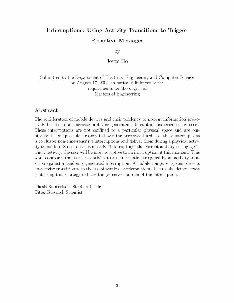
Figure 3-1: The question screens.
that the reminder is a non-time critical reminder (e.g. it does not include a reminder
to attend a meeting in 5 minutes), and the user does not have access to the caller ID
for any phone calls. The participant was asked to answer the question using a scale
of 1-5, with 1 being not at all receptive. If the user did not respond within a minute,
the iPAQ logged a “no response”. In addition, if the user tapped the screen to turn
off the sound, it was also logged as a “no response”. Even though it can be assumed
that the user was not receptive at all during this moment, it could also coincide with
an accidental tap of the screen to turn off the sound before the user heard it. There
is no way to ensure which of these two possibilities occurred without relying on the
subject’s recall ability. The rates of no response ranged from 0-28%. The average
28

rate of no response was 9.4% with a standard deviation of 7.8%.
Subjects experienced between 18-40 total interruptions spread out over the course
of the day. Each interruption required less than 10 seconds to complete. The system
either randomly generated an interruption or triggered an interruption using an ac-
tivity transition throughout the day. The system maintained a count of both types of
interruptions to ensure a balance between randomly generated interruptions and ac-
tivity transition triggered interruptions. Neither type was allowed to exceed the other
count by more than two. The algorithm would randomly generate a time between
10-20 minutes. If an activity transition occurred before the randomly chosen time,
then the activity transition would trigger an interruption unless there were already
too many of this type. However, if there had been too many random interruptions,
then the system would just wait for an activity transition.
Each participant was given two wireless accelerometers, one to be attached to the
outside of the right ankle using a small Velcro pouch and the other to the outside of
the left thigh right above the knee using an adhesive bandage. A potential subject
wearing the sensors is show in Figure 3-2. The accelerometers were manufactured to
Figure 3-2: A potential subject modeling the placement of the wireless accelerometers.
be inconspicuous, and were roughly the size of a quarter [27]. Figure 3-3 shows the
accelerometer in relation to a quarter, and the iPAQ attached to the receiver casing.
29

Participants are asked to carry the iPAQ with them at all times either in a small
pouch that attached to the belt loop or in a small travel bag.
Figure 3-3: The 3-axis wireless accelerometer (top) and the iPAQ with the receivercasing (bottom).
3.2 Procedure
The length of the study was one work day, which ranged from seven to eight hours.
Participants were given the iPAQ and the wireless accelerometers at the beginning of
their workday and instructed on how to wear them. They were also told to answer
each question based only on the particular situation at the time of the beep and asked
not to consider any previous questions. Subjects were asked to maintain their normal
work schedule. At the end of the day, a 30-minute wrap-up interview was conducted.
The details of the subject protocol are discussed in Appendix B.
30

3.3 Subjects
The study protocol was approved by the Massachusetts Institute of Technology Com-
mittee on the Use of Human Subjects. Subjects were recruited through posters placed
in the Boston area. The posters contained the following text: ”Carry a cell phone?
Help MIT Researchers learn how to design user-friendly mobile devices.” E-mails were
also sent with the same text to local mailing lists.
Twenty-five subjects (9 male, 16 female) participated in this study. Two potential
subjects were dropped from the data. One participant stopped the study because s/he
found the device too disruptive; another participant did not push the OK button
after responding to the question, preventing the system from logging any of his/her
responses. The participants were between the ages of 19 and 36, with an average
age of 25.6 and a standard deviation of 3.32. Table 3.1 illustrates the subjects’
occupations. All the subjects owned a mobile phone and were not affiliated with
the research group. The subjects carried the iPAQ for an average of 8 hours and
25 minutes with a standard deviation of 1 hour and 18 minutes. Each subject was
compensated for his/her participation with a ten-dollar gift certificate.
Occupation Number of SubjectsAdministrative Staff 3
Lab Researcher 5Office Professional 12Field Professional 4Customer Service 1
Table 3.1: Subjects by their occupation
31

32

Chapter 4
Results
The results are presented in two parts. First, evidence is presented showing that the
algorithm is capable of detecting activity transition in real-time. The results of the
interruption study follow.
4.1 Verification of Transition Detection Algorithm
The performance of the activity detection algorithm was measured against 393 phys-
ical activity transitions. Appendix H describes the process of training a C4.5 super-
vised learning classifier. The strategy used to validate the activity transition detection
algorithm was subject self-annotation. Two iPAQs were calibrated to have the same
time. One ran the activity detection algorithm, and the other iPAQ ran a simple
program that allowed the user to mark his/her activity by choosing one of the three
activity transitions. Ten colleagues who did not participate in the interruption study
were used. Five people were randomly chosen from the original ten subjects used
to train the classifier. These five subjects were asked to wear the sensors twice, the
first time to train the C4.5 classifier, and the second time to measure the classifier’s
performance. It was difficult for subjects to indicate a transition precisely when it
occurred. Provided the difference between the self-annotated transition time and the
activity transition detection algorithm time differed by no more than 10 seconds, it
was considered a valid classification.
33

A confusion matrix was calculated for each subject. In addition, confusion ma-
trices were computed for the five subjects who contributed to training data, the five
subjects who were not involved in the training process, and all 10 subjects combined.
The confusion matrices can be seen in Appendix D along with a table that summarizes
the results for these two groups.
False-positives are defined as cases in which the algorithm detected a transition
when one did not occur. Situations when physical transitions occurred but the al-
gorithm was unable to detect any transitions are considered false-negatives. Cases
are incorrectly classified when the algorithm detected another transition that was not
the same as the physical transition. The real-transition accuracy is the percentage
of real transitions the classifier was able to detect. This is calculated by dividing the
number of correct transitions the algorithm detected by the total number of physi-
cal transitions. The classifier-transition accuracy is the percentage of transitions the
algorithm correctly classified, if a transition was classified at all; it is computed by
dividing the total number of classifications into the number of correct transitions the
algorithm detected.
False- False- Incorrect Real-transition Classifierpositives negatives classifications accuracy accuracy
Mean 3.125% 12.26% 5.729% 82.55% 91.15%Standard Dev 7.89% 4.50% 3.62% 6.97% 8.71%
Table 4.1: Summary of the means and standard deviations for the activity transitiondetection algorithm evaluated on the 5 subjects not used to train the classifier.
Table 4.1 summarizes the means and standard deviations of the algorithm’s per-
formance on the five subjects not used to train the classifier. The classifier did not
perform consistently for all the subjects, as illustrated by the standard deviation.
One subject jerked his leg for a period of time, leading to a high number of false
positives. In addition, the subject acknowledge that he missed recording some of the
transitions. He specified the time at which this occurred, and any transitions during
this time period were not used in the evaluation. However, it is possible that a few
unmarked transitions remained in the data, resulting in an artificially low classifier
34

and real-transition accuracy.
False negative cases can also result in incorrect classification. If the algorithm
missed an activity transition, such as sitting to standing, but detected the change in
activity to movement, the detection algorithm will incorrectly classify the transition
as sitting to walking. The classifier had a relatively high number of false negatives in
one subject, in comparison with the other five untrained subjects. These false nega-
tives occurred because the subject transitioned before 10 seconds had elapsed for the
current activity. Since a transition is defined as an event in which a user has engaged
in the current activity for at least 10 seconds before moving onto the next activity,
this physical transition was not classified by the algorithm. The false negatives for
the subject resulted in a higher number of incorrect classifications, thereby affecting
the real-transition accuracy and the classifier-transition accuracy.
Table 4.2 summarizes the results of the activity transition detection algorithm for
all subjects. The algorithm has a higher detection accuracy for the trained subjects,
as expected. However, the accuracy only drops by 8% on untrained subjects. For
the interruption study, the key measure is the 91.15% accuracy with respect to the
classifier. The interruption experience requires a low false positive and incorrect
classification percentage. It is important that when the algorithm detects a transition
that the transition actually occurred and was correctly classified. The relatively high
number of false negatives will not affect the interruption study protocol because an
interruption will not be triggered at that particular moment. This may have resulted
in less interruptions experienced by the user, since a balance is kept between randomly
generated interruptions and activity transition triggered interruptions. Missing a
transition was not expected to skew the analysis of the data. There is the possibility
that a random interruption occurred during an activity transition. However, over the
course of the day, it was assumed that this interruption would not have a significant
effect on the overall receptivity of the user for either random interruptions or triggered
interruptions.
The algorithm’s weakness is the inability to catch all physical activity transitions.
Approximately 11% of the time, the algorithm will miss a physical transition dur-
35

False- False- Incorrect Real-transition Classifierpositives negatives classifications accuracy accuracy
Used in classifier 4.68 9.945 2.34 87.85 92.98Not in classifier 3.13 12.26 5.73 82.55 91.14
All 3.86 11.2 4.13 84.99 92.01
Table 4.2: Summary of verification results for the activity transition detection al-gorithm broken down by the subjects used to train the classifier, the subjects notrelated to the classifier, and all 10 subjects
ing the interruption study. The performance of the classifier could be improved by
loosening the restrictions on what is considered an activity transition. Since the tran-
sition requires at least 10 seconds of the previous activity and at least 3 seconds of
the current activity, a quick physical transition will be missed by the algorithm.
A consequence of the inability to capture all physical transitions is that it increases
the likelihood of incorrectly classifying the subsequent transition. As noted in the
paragraph discussing the performance anomalies for subjects unrelated to training
the classifier, the high number of false negative cases resulted in a higher incorrect
classification rate for that particular subject. The algorithm is not likely to correctly
identify the physical transition if it misses the previous activity.
In addition, any temporary classification that was used by a subject was not
detected by the algorithm because of the classifier’s definition of a physical transition.
For instance, if the subject annotated that s/he went from sitting to standing before
walking, the classifier missed the transition sitting to standing, but captured the
transition sitting to walking.
The activity transition detection may also capture high frequency or high move-
ment fidgeting. The algorithm was designed to remove as much noise from the tempo-
rary classifications as possible by requiring the previous activity to last for a duration
exceeding 10 seconds. However, there are several cases where the classifier captured
the fidgeting. Fidgeting is the source of the majority of the false-positive states.
36

4.2 Interruption Study
The number of interruptions experienced by subjects ranged from 16-48. The mean
number of interruptions was 28.8 with a standard deviation of 7.1. For plots of a
subject’s response over the course of the day, see Appendix C.
The subjects’ responses were analyzed using a paired t-test. This test was used
because it tested the difference in overall receptivity of the user between the two types
of interruption, random and activity transition triggered. The data was aggregated on
a subject level by calculating the associated means and standard deviations for each
subject [24] . Appendix I details the method of computation used for the statistical
analysis of the results.
A user’s failure to respond, or “no responses” were dealt in two different ways. The
first method involved dealing with no responses in a manner consistent with Ecological
Momentary Assessment (EMA) or Experience Sampling Methods (ESM) [24]. “No
responses” were not used in the computation. This method was appropriate since
it was unknown whether the user failed to answer the question because s/he was
unreceptive or because s/he did not hear the audio prompt. The second method
involved treating a “no response” as “extremely unreceptive”. The analysis was
computed with no responses taking on the value of 1, which represents not at all
receptive. The assumption in this case was that the user was unable to respond to
the question and was therefore not at all receptive to an interruption.
The accuracy of the classifier was simulated by randomly removing 9% of the
activity transition responses and changing them to be random interruptions. 9% was
obtained by taking 100% and subtracting off the classifier accuracy of the algorithm
on subjects who did not train the classifier as noted in the previous section, which
was 91.15%. In addition, the worst case scenario was simulated by equating the
accuracy of the classifier to 82.44%, one standard deviation below the average classifier
accuracy.
The aggregated data was analyzed using several separate two-tailed paired t-tests.
The t-tests used a confidence interval of 95% with a significance level of p = 0.05.
37

The upper bound and lower bound for the confidence interval mark the boundaries
where the expected difference in means of 95% of the population to fall. Any signif-
icance level lower than 0.05 with a confidence interval that does not intercept zero
corresponds to a significant result. A confidence interval that contains zero signifies
that there is no difference in the means. The expected mean of the entire popula-
tion, if it was sampled, would lie in the boundaries of the confidence interval with
a probability of 0.95. Appendix D contains the complete outputs of the statistical
analysis for all t-tests performed. Table 4.3 summarizes the results of the paired t-
tests using a classifier accuracy of 91.15%, while Table 4.4 summarizes the worst case
scenario. Finally, Table 4.5 contains the mean and standard deviation of the number
of triggered interruptions experienced by the subjects.
Lower Bound of Confidence Interval Upper bound of Confidence Interval Significance“NO RESPONSES” OMITTED
All responses -0.52 -0.24 <0.001Phone calls only -0.45 0.024 0.076Reminders only -.82 -0.32 <0.001Male subjects -0.55 -0.19 0.002
Female subjects -0.59 -0.18 0.001“NO RESPONSES” INCLUDED
All responses -0.47 -0.19 <0.001Phone calls only -0.54 -0.10 0.007Reminders only -0.82 -0.32 <0.012Male subjects -0.48 -0.10 0.009
Female subjects -0.55 -0.14 0.003
Table 4.3: Summary of paired t-tests results for a classifier with 91.15% accuracy
Lower Bound of Confidence Interval Upper bound of Confidence Interval Significance“NO RESPONSES” OMITTED
All responses -0.53 -0.20 <0.001Phone calls only -0.71 -0.05 <0.001Reminders only -0.85 -0.17 0.005Male subjects -0.65 -0.05 0.027
Female subjects -0.59 -0.12 0.005“NO RESPONSES” INCLUDED
All responses -0.43 -0.06 0.010Phone calls only -0.69 -0.07 0.017Reminders only -0.51 0.04 0.092
Sitting to walking transitions -0.71 -0.09 0.013Sitting to standing transitions -0.25 0.66 0.355Walking to sitting transitions -0.65 0.18 0.063Standing to sitting transitions -0.62 0.09 0.135
Male subjects -0.69 0.06 0.086Female subjects -0.48 -0.04 0.022
Table 4.4: Summary of paired t-tests results for a classifier with 82.44% accuracy
The results indicate a significant increase for activity triggered responses compared
to random responses, p <0.05. This significant increase in activity triggered responses
is independent of the manner in which “no responses” were treated. In addition,
38

Triggered Triggered Phone Reminder Phone Reminder91% 82% 91% 82% 91% 81%
Mean 12.6 11.4 6.8 5.8 6.3 5.1Std.Dev 3.6 3.3 2.9 2.4 2.7 2.4
Table 4.5: The means and standard deviations for the number of triggered responsesexperienced by the subjects broken down by the classifier accuracy
this difference holds for the worst case scenario, in which the classifier performs one
standard deviation below the expected accuracy.
The results also indicate a significant increase for activity triggered responses
with respect to the reminder, p <0.05. The difference is significant for both the
average and worst case scenarios of the classifier accuracy. However, the results only
indicate a significant increase for activity triggered responses with respect to the
phone call with the worst case scenario, where the classifier accuracy is 82%. The
results do not indicate a significant increase for the activity transition triggered phone
call interruptions in the average simulated performance of the classifier.
In the wrap-up interview, subjects were asked to estimate the number of inter-
ruptions they experienced and whether they would recommend the study to a friend.
The rationale behind both questions was that if the subject was irritated by the
study, s/he would overestimate the number of interruptions experienced and choose
not to recommend the study to a friend [15]. The mean for the difference between the
number of estimated interruptions to actual interruptions was -1.76 with a standard
deviation of 16. The range was -14 to +71. One participant estimated 100 interrup-
tions when s/he had only experienced 29. 19 of the subjects would recommend the
study to a friend. The remaining six subjects were split between not recommending
the study at all and possibly recommending the study.
The subjects also had differing values of the two types of interruptions. Nine of
the 25 of the participants favored a reminder while the remaining 16 preferred phone
calls. Most subjects who favored the reminder estimated an average phone call to
take at least 10 times as long as a reminder. In addition, only two of the 25 subjects
muted the study. Both subjects muted it for a total of one hour.
39

40

Chapter 5
Discussion and Future Work
The results support the strategy of using activity transitions as a trigger for non-time-
critical interruptions. This study suggests that by delaying interruptions that are not
time-sensitive and marking them for delivery during a physical activity transition, the
user may be more receptive towards these interruptions. We have also shown that
two 3-axis wireless accelerometers can reliably detect a user’s activity transition real
time and be used for interruption triggering.
In addition, the results also suggest that the utility of message has an effect on
the receptivity of the user. Users may be more receptive towards activity transition
triggered reminders, whereas there may not be a difference in receptivity to activity
transition triggered phone calls. However, this outcome may be skewed by the num-
ber of triggered responses for each type of message. As noted in Figure 4.5, the mean
number of triggered responses in the average classifier scenario is 6.8 for phone calls
and 5.8 for reminders. Furthermore, the standard deviation for the two responses are
2.9 and 2.4. This suggests that in the worst situation, a subject may have experi-
enced less than four triggered phone call interruptions and four triggered reminder
interruptions. If a subject answered any of the interruptions with an extreme rating
(either 1 or 5), this could drastically alter the mean of the response for that particular
subject. This could be a possible explanation for the difference in significance levels
between the two different classifier accuracies. There is a possibility that when activ-
ity transition responses were removed for the 91% classifier accuracy simulation, the
41

more receptive responses may have been removed. It is also possibile that in the 82%
accuracy simulation, the unreceptive responses were randomly selected to be removed
Either of these two situations could alter the significance level of the paired t-tests.
Regardless of the type of interruption, subjects’ responses were generally lower
when they were talking to their supervisor. The warp up interviews frequently in-
dicated that the reasoning for choosing 1 was that the participant was talking to
his/her supervisor. Using an activity transition as a trigger of interruptions should
avoid scenarios when both the manager and the subject are sitting at the desk, but it
does capture the situation when a subject gets up to walk to the manager’s office and
sit back down. Subjects were also asked whether an interruption of a different type
(maybe breaking news, an e-mail message, or an exercise to de-stress) or a different
medium of delivery would make a difference. Some subjects responded positively to
the use of vibrations to notify the user of the interruption, making the situation less
socially awkward, but acknowledged that they still would be unable to respond to
the interruption immediately.
Lab researchers in particular complained that an interruption would occur while
they were conducting an experiment. Two participants reported that they had to
remove their gloves to answer the questions. A few lab researchers had considered not
carrying around the iPAQ because they were involved in work that required precise
measurements and could not afford to be interrupted. Additionally, another lab
researcher noted that s/he was interrupted more frequently during an appointment
with a patient. The reason for the higher frequency was due to the fact that the
researcher often walked to attend to the patient and then sat down to perform tests
multiple times during the appointment, signaling an interruption. This situation
would require additional sensors to detect the presence of a patient since the strategy
of using an activity transition as a trigger was not appropriate.
One of the office professionals also noted that when s/he was less receptive, the
iPAQ seemed to deliver interruptions at a higher frequency. The subject then de-
scribed that s/he was leading a board discussion with several coworkers and clients
and was frequently interrupted during this period. In this particular scenario, the
42

subject stood to write on a white-board but then sat back down to continue the
discussion with the rest of the group.
Several subjects commented on the interruption occurring while the subjects were
driving on the road. One to two of the subjects stated that this was actually a good
time for an interruption because they were just driving, but other subjects considered
this a distraction and that they needed to focus on driving and not answering a phone
call or reading a reminder.
When subjects were informed the nature of the study, 5-6 subjects noted that the
algorithm should consider monitoring their computer since there were periods during
the day when they had nothing to do and were surfing the Internet. They described
these moments as times when they would be extremely receptive to any interruption
since it would keep them occupied.
Several challenges arose during the interruption study. The first challenge was
determining the statistical test needed to analyze the data. Since ESM and EMA are
relatively new fields of study, this area of research has not established a consistent
method of analysis [24]. The difficulty with analyzing this data is the presence of
multiple observations per subject that are not consistent between subjects. Many
standard statistical techniques are usually appropriate given that the data has been
aggregated on the subject level. The techniques vary to encompass the differences in
experiments. Furthermore, prior work seemed to favor the use of Analysis of Variance
(ANOVA) or the paired t-test [1, 15] as a measure of significance. As a result, the
paired t-test was chosen as a means for analyzing the data. Appendix I discusses
the potential problems with using the paired t-test.
The false-positive transitions that resulted from fidgeting were also a concern. To
minimize falsely detected transitions, the definition of a transition was set to require
at least 10 seconds of the previous activity and approximately three seconds of the
current activity. However, this does not prevent fidgeting from being detected. If
a subject fidgets constantly, then the algorithm might detect the wrong transitions.
A possible solution is to make the sampling window 512 (or 5.12 seconds) with an
overlapping window of 256. This larger sampling window allows the decision tree
43

to capture more activities, possibly building a better representation of the different
activities. Another solution would be to train the classifier with more examples of
subjects fidgeting while they sit or stand.
One of the initial subjects used headphones while participating in the study. The
headphones prevented the subject from hearing the audio prompt, and the subject had
to be notified by neighboring coworkers that the iPAQ was signaling an interruption.
As a result, the subject answered “extremely unreceptive” to these interruptions
because of the possible disruption to bothered his coworkers. During the wrap-up
interview, the subject stated that the disruption of the interruption experienced by
the coworkers did not change his receptivity rating because he was preoccupied at
the moment. Furthermore, this subject did not skew the data towards favoring the
activity transition triggered interruptions. The significance level of the paired t-test
remained at p <0.05 excluding this subject. Future subjects were notified to avoid
the use of headphones for the day.
One potential subject left the study before an hour had elapsed. The subject
objected to the study because she found the interruptions too disruptive. The subject
noted that since she served as an administrative assistant for multiple supervisors, she
was constantly working on something urgent. The participant also suggested that had
her job entailed “mindless work”, the interruptions would not have been disruptive
since the chimes were quite pleasant.
Another potential subject ran the experiment for the day but her data was un-
usable because she failed to push the OK button after responding to the question.
Even though the subject was walked through the graphical interface at the beginning
of the day, she assumed that pushing the hardware buttons on the iPAQ would be
equivalent to hitting the OK button. As a result, the system logged all the responses
as a “no response” since the subject failed to complete a question.
The battery life of the accelerometers impacted one subject who had a shortened
workday studied because one of the batteries inserted into the accelerometers was
defective and only lasted for approximately 6 hours. However, because of the ac-
tive nature of his/her job, the subject still experienced 20 interruptions during this
44
condensed workday.
Maintaining a consistent number of interruptions was another challenge. As noted
in the results section, the number of interruptions experienced by the subjects differed
by more than 30 interruptions. Some subjects spent the time primarily at their desk
and would only leave the desk intermittently. Other subjects would constantly be
moving, running errands every 10-15 minutes. As a result, these subjects would
trigger more activity-transition interruptions. In addition, the workdays varied in
length from seven to nine hours depending on the occupation. One participant wore
the iPAQ and sensors for over 12 hours because s/he had a dinner meeting that
particular day. Furthermore, even though subjects were provided carrying cases for
the iPAQ, sometimes they would forget to bring the iPAQ with them, causing the
wireless accelerometers to go out of range.
Subjects also commented that it was difficult to differentiate the two types of
questions, the phone call and the reminder. They would have liked the system to
signify the difference in type through a different set of chimes. Additionally, five
subjects stated that they did not use reminders and found it difficult to rate their
response because they had no previous experience to base their receptivity towards
the reminder.
Finally, it should be noted that even though the results suggest that activity tran-
sition triggered interruptions may lead to a lower perceived burden on the user, it has
yet to be determined the overall effect is on the user. Although the users reported be-
ing more receptive towards activity transition triggered interruptions, this preference
might not be observed over time. For instance, a user might receive 100 interruptions
over the course of a week, be s/he might only notice the extreme cases where the
device interrupted him/her at an inconvenient moment. The user might only remem-
ber these extreme cases and not realize that s/he was more receptive towards the
interruptions overall as opposed to the device randomly generating interruptions.
In the future, the experiment could be extended to examine the effect of different
activity transitions and the utility of message on the user’s perceived burden of inter-
ruption. The work could incorporate other types of activities (i.e reading, cooking,
45

cleaning) and extend beyond the office environment. A larger set of message types (i.e
phone call, instant message, or breaking news) could be used to determine whether
there is a correlation between the type of message and the activity transition used
to trigger the interruption. Subjects could be asked to wear the sensors for 14-16
hours starting from the moment they awaken for more than three days. This would
allow the subject to become acclimated to the sensors and the interface. Furthermore,
this experiment could determine if it is necessary to have a trainable algorithm that
will allow the user to determine which activity transitions trigger a certain type of
message or if a generic algorithm would be sufficient for the general population.
46

Chapter 6
Conclusion
An interruption timed at a transition between two physical activities may be perceived
as less burdensome than an interruption presented at a random time. A change in
physical activity may sometimes correlate with a self-initiated mental transition and
therefore increases the receptivity of the user towards an interruption. This study
found that the user is more receptive towards an activity transition triggered interrup-
tion when triggered by a change in physical activity. The implication of this result is
that non-time-critical interruptions to be delivered to users by mobile computing de-
vices that are clustered and marked for delivery during a physical activity transition,
may minimize the perceived burden of interruptions experienced by users.
47

48

Appendix A
Prior Work and Additional Details
Prior literature relating to the model of interruption is detailed below. This section
summarizes the findings of recent works that have contributed to the eleven factors
of the model of interruption used in this work.
A.1 Activity of the User
The disruptiveness of an interruption is influenced by the similarity of the interruption
task to the primary task. The closer in similarity the interruption task is to the
primary task, the more disruptive the interruption may be, where the disruption is
measured as the length of time necessary to complete the tasks [5].
In addition, the effect of an interruption is influenced by the training level of the
primary task. If a user is highly trained on a primary task without interruptions,
an interruption presented during a later session is often significantly harmful to the
performance. However, if a user is trained on a primary task for two sessions with
the interruptions, by the third session the interruption will be less disruptive [6]. The
activity of the user is also directly correlated to the memory load. If the memory load
during the primary task was high, then it would be difficult to resume the original
activity after completing the interruption activity [1]. A schedule and sensor data
can be used to formulate the probability of the user actually initiating in a particular
activity, helping determine the interruptability of the use [17].
49

The timing of the interruption during the activity also governs the effect of the
interruption. In a previous study, interruptions that occurred during the execution
stage of a task was more disruptive to the performance [4]. The time at which the
interruption occurs during the activity influences the effects of the interruption [6].
A.2 Utility of Message
The utility of the information is determined by the importance of the message re-
ceived or requested. Utility of information is composed of the task referential (the
relevancy to the original activity/task of the user), the importance of the message
to the user, and the commitment of the user to the message, determined by a previ-
ous engagement with the originator of the message. Interruptions that are relevant
to the ongoing activities are less disruptive to the user [4]. The Scope notification
system emphasizes the importance of a message. It calculates the importance based
on several parameters such as the composition of the message, the subject heading,
the recipient of the message, the sender the message, etc. The interface then displays
the importance of the message by the distance from the center of the circle to the
blinking notification. The interface is visible to the user at all times, but does not
fill the entire screen [28]. This factor is difficult to detect as each person may have
varying views on the importance of the same message.
A.3 Emotional State of the User
Another aspect of a user’s response to an interruption is his/her emotional state. The
emotional state of the user comprises of the time of the disruption, the mindset of the
user, and the relationship the user has with the device or interface. The time of an
interruption was significant in determining a user’s attitude toward interruptions [29].
It was also shown that openness to an interruption varied regularly based on the
time of the probe, and these strong attitude patterns differed from individual to
individual [12]. The user’s current state of mind also influences the emotional state
50

of the user. For instance, if a user is stressed and has immediate deadlines, s/he
may not be open to interruptions. One method of inferring the users attention used
the time of day and proximity of deadlines in addition to the user’s schedule [9]. It
has been demonstrated that cues to our emotional state can be measured using basic
physiological parameters, and context-aware applications can use these cues as input
to an recognition algorithm [16].
A.4 Modality of the Interruption
Modality, the choice of interface in which to interrupt the user, is yet another aspect
of interruption. The importance of modality was explored in a study that asked
eight main questions regarding interruptions. The study was distributed to work
groups in two organizations and consisted of questions such as the medium in which
interrupts occur, the underlying reasons for interrupts, and the recovery time after
interrupts [29]. If the modality was similar to the current activity, the users ability
to multi-task with the interruption and the current activity is minimized since it
creates a cognitive overload. Generally, the most disruptive modalities were smell
and vibration [26]. However, interruptions delivered through graphical displays have
been found to enhance decision making [23]. The cost of the interruption needs
to include the cost associated with the different modalities to determine the best
modality for the interruption [10].
A.5 Frequency of Interruptions
The model of interruption also includes the frequency of an interruption. If the
interface interrupts the user at a low frequency, the chances of the message occurring
at an inconvenient time are less likely than high frequency disruptions. High frequency
interruptions were found to be disruptive [23], measured by a user’s inability to return
to the original task and complete it in a timely fashion. The high frequency may result
in the user constantly switching tasks thereby creating a higher memory load.
51

A.6 Comprehension Rate and Expected Length of
the Interruption
The task efficiency rate, or the comprehension rate and the expected length of inter-
ruption can induce the user to respond to the interruption in different ways. It was
found that the actual length of a interruption cannot be used to determine the detri-
mental effects of the interruption [6]. However, this particular study interrupted the
user’s main activity with a long but simple interruption. If the user had experienced
the interruption previously and was able to estimate the time needed to complete
the interruption task, a longer task might be more disruptive since it would require
a larger memory load. In addition, a complex interrupted task caused a cognitive
overload, distracting the user from the original task and requiring more time to deal
with the interruption [23], making it harder to comprehend the task at hand.
The medium of an interruption can contribute to the comprehension and task
efficiency rate. A user might spend more time in comprehending the task with a
text message in comparison to a verbal message. One system found that graphical
displays enhanced the decision-making when complex activities are interrupted [23].
The Scope notification system used visual cues to signal the arrival of a message. The
creators noted that the limitations of a visual interface are the difficulties in designing
simple visual annotations to convey the information and the need to train the user
on the interface [28].
A.7 Authority Level
The perceived level of authority the user has over the interface/device also contributes
to the effects of an disruption. If the user believes that he/she has a certain level
of control over the schedule of interruptions, there will be a higher level of tolerance
since the user has a notion that the interruption was triggered by his/her own ac-
tion. Users were more open to interruptions when they maintained control over the
interruptions [12]. A study conducted at Lawrence Livermore National Laboratory
52
explored the differences between an on-screen computer interruptions and telephone
interruptions. Subjects were asked to complete a form as their main task. They were
interrupted at random times with a telephone call, a modal dialog on-screen, and a
personal visit. This study found that the abruptness of the onset of the on-screen
modal dialog interruption prohibited the subject from completely the task at hand,
while the telephone and personal visit allowed the user to determine when to field the
interruption [25].
A.8 Previous and Future Activities of the User
The previous and future activity comprises another factor of the model. If the previous
or future activity requires a large memory load, the user may engage in a lower
memory task at the moment. In addition, the previous activity information can be
used to construct a model relevant to that particular user. One study constructed a
Bayesian network that was able to reason about the current state of interruptability
and forecast future state of interruptability using a training data set. This network
used acoustic and visual analysis to detect the presence of conversational or non-
conversational sounds related to the activity of the user and the presence of the
user in the workspace. In addition, it tracked the input to the computer (keyboard,
mouse), task completion of programs, and the schedule of the user. Using these
inputs, the network predicted the state of the interruptability and forecasts the time
until the following opportune time of high, medium, lower interruptability using the
history of interaction and the activity of the user at the current time [8].
A.9 Social Engagement of the User
A user’s social engagement is determined by his/her role in the current activity. If the
user is the speaker at a talk, then his/her social engagement is high and should not
be interrupted. Using audio and location sensors, one study determined the social
engagement of the user with an accuracy of 94.6% [14].
53
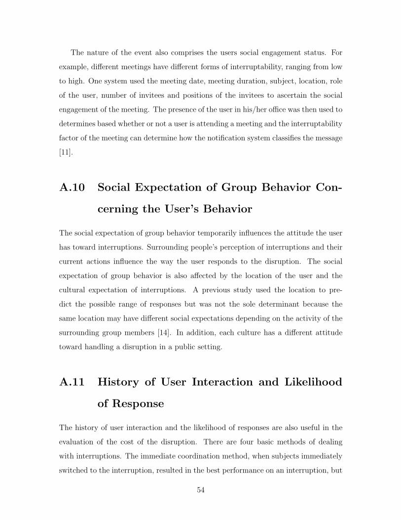
The nature of the event also comprises the users social engagement status. For
example, different meetings have different forms of interruptability, ranging from low
to high. One system used the meeting date, meeting duration, subject, location, role
of the user, number of invitees and positions of the invitees to ascertain the social
engagement of the meeting. The presence of the user in his/her office was then used to
determines based whether or not a user is attending a meeting and the interruptability
factor of the meeting can determine how the notification system classifies the message
[11].
A.10 Social Expectation of Group Behavior Con-
cerning the User’s Behavior
The social expectation of group behavior temporarily influences the attitude the user
has toward interruptions. Surrounding people’s perception of interruptions and their
current actions influence the way the user responds to the disruption. The social
expectation of group behavior is also affected by the location of the user and the
cultural expectation of interruptions. A previous study used the location to pre-
dict the possible range of responses but was not the sole determinant because the
same location may have different social expectations depending on the activity of the
surrounding group members [14]. In addition, each culture has a different attitude
toward handling a disruption in a public setting.
A.11 History of User Interaction and Likelihood
of Response
The history of user interaction and the likelihood of responses are also useful in the
evaluation of the cost of the disruption. There are four basic methods of dealing
with interruptions. The immediate coordination method, when subjects immediately
switched to the interruption, resulted in the best performance on an interruption, but
54

as a consequence, there was a loss of decision accuracy in the original activity. The
negotiated coordination involved delaying an interruption, provided better accuracy
with the original task, but the disruption was postponed for a period of time. In the
case of schedule coordination, it required the least amount of task switches since the
interruptions were all scheduled, but the accuracy was horrible for a continuous task.
Mediated solutions or notification systems, produced average levels of performance
accuracy in all aspects [19]. History of the sensor data also helped maintain smooth
transitions as brief changes in environment data would cause a change in transition
[22].
55

56

Appendix B
Subject Protocol
Details for subject recruitment and the interruption experiment protocol are provided
below. The study was approved by the MIT Committee On The Use of Humans as
Experimental Subjects.
B.1 Recruitment
Flyers publicized the need for research subjects. The flyers had a headline that said:
”Carry a Cell Phone?” Each poster then contained the following description:
Help MIT Researchers learn how to design user-friendly mobile devices.
Earn a $ 10 gift certificate without even leaving your office. Must be over
18. Contact Joyce at [email protected] or 617-452-5604.
In addition, the same flyer was advertised on boston.craigslist.com under the volun-
teers section.
When a person responded to the ad, s/he was given a general description of the
study over the phone. The duration of the study was a workday, approximately 7-9
hours. The participant would need to wear two motion sensors (wireless accelerome-
ters) on their legs, and carry around a PDA for the day. The PDA would prompt the
user for information every 3-5 times an hour, with each interruption requiring less
than 10 seconds of the participant’s time. The researcher would meet the participant
57

in the morning at his/her workplace to deliver the materials, go over the specifics of
the study, and arrange a time in the evening to pick up the material and engage in a
15-30 minute wrap-up interview. Subjects who agreed to the protocol were scheduled.
Only 1 subject chose to come to our office, the remaining 24 subjects requested to
meet the researcher at their workplace.
B.2 Subject Preparation
In the morning on the scheduled day, participants were asked to sign an informed
consent to document their agreement to participate in the study. At this time, par-
ticipants were informed that any data collected from the study would be disassociated
with their actual identities and that they had the option to stop the study at any
time. Subjects were asked the following demographic questions to obtain a better
understanding of their data:
1. What year were you born?
2. What is your profession?
3. Can you please describe your normal workday?
4. Do you own a cell phone, digital camera, or PDA?
5. Do you instant message?
Then, participants were shown the wireless accelerometers and the PDA that would
be in their possession for the day. The researcher walked the participant through a hy-
pothetical interruption using Figures B-1, B-2, B-3 as visual aids. The researcher then
attached the accelerometers to the participant and talked the participant through the
first real interruption. The researcher stressed that the questions should be answered
independently of all previous situations. If the subject felt it was absolutely necessary
to mute the experiment, they had the option to do so on the start screen. The back
of the iPAQ contained a cheat sheet of the icons and the interpretation of the scale
58

as well as the researcher’s contact information. The back of the iPAQ is illustrated
in Figure B-4.
Figure B-1: The visual aid used to explain the mute screen and the start screen.
Figure B-2: The visual aid used to explain the icons used in the question screen.
B.3 Wrap-up Interview
At the end of the day, the researcher met the subject for a post-experiment interview.
The participant was asked the following questions:
1. Did anything out of the ordinary happen during the work day?
2. To the best of your ability, how many times did the PDA interrupt you today?
59
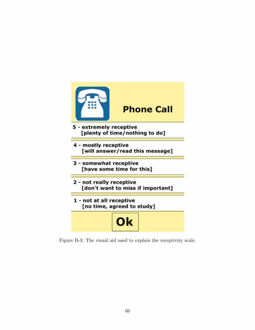
Figure B-3: The visual aid used to explain the receptivity scale.
60

Figure B-4: The cheat sheet that is attached to the back of the wireless casing.
61

3. Did you find yourself becoming more or less receptive towards the interruptions
over the course of the day?
4. Can you put in your own words how you were interpreting each of the numbers,
and what it meant in terms of your interruptability?
5. Could you tell me how you interpreted the meaning of each of the icons [for
example the type of reminder you associated with the question]?
6. Which type of interruption are you most receptive to at any given point during
the day?
7. How much time would it take to respond to each interruption typically (in
minutes)?
8. This is a chart of how you answered your questions (see Figure C-1)
(a) The first time you answered a [value]. Can you describe the situation?
(b) The last time you answered a [value]. Can you explain the rating?
(c) At this time, you answered a 1. Could you tell me what was going on
then?
(d) At this time, you answered a 5. Can you recall what went into the situa-
tion?
(e) Why did you mute the survey at this time?
(f) At this moment, it took you much longer to respond to the question, was
there a particular reason?
9. In the situation where you answered a 1, do you think if the interruption had
used a vibration or a visual prompt as the initial interruption it would have
been better? Can you think of a different way that it could have interrupted
you so that you would have been more receptive?
10. In the situation where you answered a 1, do you think you would have been
more receptive to an interruption of a different type?
62

11. Would you recommend this study to a friend?
12. How can we improve the comfort level of the sensors?
13. Did you notice any pattern behind the interruptions?
14. How did people around you respond to the system when an interruption oc-
curred?
15. What did you tell your colleagues about your participation in the study if they
asked?
16. Do you have any questions or comments on the study? Would you like me to
tell you more about how the interruptions were determined? Let me know if
you have any more questions.
Each participant received a $10 gift certificate to Dunkin Donuts at the end of the
study.
B.4 Accelerometer Placement
The accelerometers are placed on the subject through the use of an adhesive bandage
and a custom-made velcro pouch. Each accelerometer is placed in an anti-static bag
surrounded by clear packing tape to make the pouch water-resistant and includes a
label in case the accelerometer is lost. The bandage is labeled with a drawing and
text to help orient the accelerometer placement. The accelerometer is attached to
the adhesive using velcro. Figure B-5 shows a picture of the accelerometer pouch, a
labeled bandage, and the velcro pouch for the ankle.
The accelerometer is placed on the adhesive such that it lines up with the dia-
gram. The participant is then asked to place the bandage on the outside thigh of
the left knee. Figure B-6 shows the adhesive with the attached accelerometer and a
participant putting on the bandage.
63

Figure B-5: The housing for the sensors, the adhesive bandage, and the velcro pouch.
Figure B-6: A participant placing the bandage in the correct orientation and place-ment.
64

Appendix C
Sample Data Set
This section describes the data set associated with each subject and the 4 different
plots that the subjects were shown during their wrap-up interview. Each subject
generated 7 different files from their participation in the study. The 7 files are listed
below:
1. The dataLog file contains the raw accelerometer data. This is kept in case there
is a need for post-processing of the subject’s data. The data log is compressed
to save storage space on the iPAQ and needs to be uncompressed to view the
data. The raw accelerometer data for all the subjects are located in Experiment
Data\accelData.
2. The featureLog file stores all the features calculated in real-time and the clas-
sification for each sampling window. This has also been compressed because of
the frequency of the feature calculation. A program was written to convert the
featureLog into a comma-delimited file. These files are located in Experiment
Data\featureData.
3. When the classification for a sampling window is written into the featureLog
file, it uses the integer number to save space. The tree-mapping.csv file saves
the mapping the classifier uses to map the integer classification to the string
classification. The files can be found in Experiment Data\treeMapping.
65

4. The experiment.dat file maintains the user’s response to the interruptions over
the course of the day. Each response is broken down by the hour, minute,
second, question type, response, time to tap the screen, time elapsed, mute
on, trigger, previous activity, and current activity. For the question type, a 0
represents a phone call while a 1 signifies a reminder. A 1 in the trigger type
represents an activity transition trigger, while a 0 means the interruption was
randomly generated. Matlab scripts have been written to view the data from
the subject. The experiment files can be found in Experiment Data\responses.
The Matlab scripts are located under Experiment Software\matlab.
5. The log.txt file contains the log of the program and can be used to troubleshoot
problems in the program. All these files are placed in the following directory:
Experiment Data\logFiles
6. The start-interview.doc has the demographic information for each subject. The
demographic information is also summarized in an excel file. The location for
these files are Experiment Data\demographicInfo.
7. Finally, the post-interview.doc contains the subject’s responses to the wrap-up
interview and any comments that s/he may have made. These files were placed
in the Experiment Data\interviewData directory.
The subject is shown four graphs during their wrap-up interview. The graphs are
used to obtain a better understanding of the situation. Sometimes the subject would
have slight difficulties recalling the exact situation involving the extreme cases, but
the majority of the subjects managed to recall the situation after some time. These
four graphs the subject saw are:
1. Time vs. Receptivity Response
2. Time vs. Response Time (measured between the user tapping the screen to
pressing OK)
3. Time vs. Mute On (check to see if the mute was on)
66

4. Time vs. Question Type
An example of the graphs that were viewed by one subject can be seen in Figures C-
1, C-2, C-3, and C-4. In Figure C-1, a dotted rectangle is used to highlight the cases
in which the subject answered that he/she was not very receptive in an effort to direct
the discussion towards those situations. In Figure C-3, a response time of 60 seconds
occurs when the user does not respond to the chime. A response time of 90 seconds
signifies that the user tapped the screen, but did not respond to the question.
Figure C-1: A plot of the subject’s response over the course of the day
67

Figure C-2: A plot of the subject’s response time over the course of the day
68

Figure C-3: A plot of whether the subject chose to mute the study over the course ofthe day
69

Figure C-4: A plot of what types of questions the subject was asked over the courseof the day
70

Appendix D
Additional Result Details
This section contains additional result details for the verification of the accuracy of
the transition tests and the experiment study results.
D.1 Verification of Activity Transitions
The confusion matrices for the activity transition detection algorithm are shown be-
low from Table D.1 to Table D.13. This data was gathered using self-annotated
transitions. The tables contain all 10 subject’s confusion matrices, and the confusion
matrices for subjects who contributed to the training data (Group 1), subjects who
did not contribute to the training data (Group 2) and both groups combined. Table
D.14 summarizes the percentage for each individual, the two groups (Group 1 and
Group 2), and both groups combined.
Real TransitionsClassifier Transitions sit-walk sit-stand walk-sit walk-stand stand-sit stand-walk no transition
sit-walk 2 1sit-stand 3walk-sit 2
walk-stand 10stand-sit 3
stand-walk 9no transition 3 2 2
Table D.1: The confusion matrix for subject 1 from Group 1.
71
Real TransitionsClassifier Transitions sit-walk sit-stand walk-sit walk-stand stand-sit stand-walk no transition
sit-walk 2 1sit-stand 1walk-sit 3 1
walk-stand 4stand-sit
stand-walk 5no transition
Table D.2: The confusion matrix for subject 2 from Group 1.
Real TransitionsClassifier Transitions sit-walk sit-stand walk-sit walk-stand stand-sit stand-walk no transition
sit-walk 2 1sit-stand 3walk-sit 2
walk-stand 12 1stand-sit 5
stand-walk 1 8 1no transition 1 1
Table D.3: The confusion matrix for subject 3 from Group 1.
Real TransitionsClassifier Transitions sit-walk sit-stand walk-sit walk-stand stand-sit stand-walk no transition
sit-walk 2sit-stand 6walk-sit 4
walk-stand 13 2stand-sit 3
stand-walk 16 2no transition 1
Table D.4: The confusion matrix for subject 4 from Group 1.
Real TransitionsClassifier Transitions sit-walk sit-stand walk-sit walk-stand stand-sit stand-walk no transition
sit-walk 4sit-stand 6walk-sit 8
walk-stand 8stand-sit 1
stand-walk 1 12no transition 1 3 2 2
Table D.5: The confusion matrix for subject 5 from Group 1.
Real TransitionsClassifier Transitions sit-walk sit-stand walk-sit walk-stand stand-sit stand-walk no transition
sit-walk 12 2 1sit-stand 19walk-sit 19 1
walk-stand 47 3stand-sit 12
stand-walk 2 50 3no transition 1 3 3 4 3 4
Table D.6: The confusion matrix for all subjects in Group 1.
Real TransitionsClassifier Transitions sit-walk sit-stand walk-sit walk-stand stand-sit stand-walk no transition
sit-walk 3 2sit-stand 1walk-sit 2 1 1
walk-stand 1 9 1stand-sit 1
stand-walk 10 2no transition 2 2
Table D.7: The confusion matrix for subject 1 in Group 2.
72

Real TransitionsClassifier Transitions sit-walk sit-stand walk-sit walk-stand stand-sit stand-walk no transition
sit-walk 1 2sit-stand 5walk-sit 4 1
walk-stand 17stand-sit 3
stand-walk 20no transition 1 2 1
Table D.8: The confusion matrix for subject 2 in Group 2.
Real TransitionsClassifier Transitions sit-walk sit-stand walk-sit walk-stand stand-sit stand-walk no transition
sit-walk 2sit-stand 6walk-sit 5 1
walk-stand 12stand-sit 1 2
stand-walk 15no transition 1 1 1 2
Table D.9: The confusion matrix for subject 3 in Group 2.
Real TransitionsClassifier Transitions sit-walk sit-stand walk-sit walk-stand stand-sit stand-walk no transition
sit-walk 4sit-stand 3walk-sit 5
walk-stand 6stand-sit 2
stand-walk 7no transition 2 1 1 2
Table D.10: The confusion matrix for subject4 in Group 2.
Real TransitionsClassifier Transitions sit-walk sit-stand walk-sit walk-stand stand-sit stand-walk no transition
sit-walk 5 2sit-stand 5walk-sit 9 2
walk-stand 3stand-sit 2
stand-walk 6no transition 1 1 4 1
Table D.11: The confusion matrix for subject 5 in Group 2.
Real TransitionsClassifier Transitions sit-walk sit-stand walk-sit walk-stand stand-sit stand-walk no transition
sit-walk 15 4 2sit-stand 20walk-sit 25 4 1
walk-stand 1 47 1stand-sit 2 10
stand-walk 58 2no transition 2 4 1 10 1 8
Table D.12: The confusion matrix for all subjects in Group 2.
Real TransitionsClassifier Transitions sit-walk sit-stand walk-sit walk-stand stand-sit stand-walk no transition
sit-walk 27 6 3sit-stand 39walk-sit 44 4 2
walk-stand 1 94 4stand-sit 2 22
stand-walk 2 108 5no transition 3 7 4 14 4 12
Table D.13: The confusion matrix for all subjects in both groups.
73

False-positive False-negative Incorrect classification Real-transition accuracy Classifier accuracyGROUP 1Subject 1 0% 18.92% 3.33% 78.38% 96.67%Subject 2 11.76% 0% 0% 100% 88.24%Subject 3 5.56% 5.56% 5.56% 88.89% 88.89%Subject 4 8.33% 2.22% 0% 97.78% 91.67%Subject 5 0% 16.67% 2.5% 81.25% 97.5%GROUP 2Subject 1 17.65% 12.5% 5.88% 81.25% 76.47%Subject 2 0% 7.02% 5.66% 87.72% 94.34%Subject 3 0% 10.42% 2.33% 87.5% 97.67%Subject 4 0% 17.65% 3.57% 79.41% 96.43%Subject 5 0% 17.07% 11.76% 73.17% 88.24%Group 1 4.68% 9.95% 2.33% 87.85% 92.98%Group 2 3.13% 12.26% 5.73% 82.55% 91.15%
Both groups 3.86% 11.2% 4.13% 84.99% 92.01%
Table D.14: Summary of the results from the activity transition detection verificationtests.
D.2 Experiment Study Results
Tables D.15 through D.23 are the outputs of the statistical analysis software after
running the paired t-tests for a three different classifier accuracies. The paired t-test
output is the most important of the tables because it illustrates whether the difference
between the means was due to chance.
For the paired samples statistics output, the mean refers to the average mean of
the responses, n is the number of cases, std. deviation is the standard deviation of
the means, and finally the last column is the standard error for a pair of variables.
This table can be used to verify the paired t-test output as well as obtain a better
understanding of how the calculations for the paired t-test were derived. In the paired
samples correlations, n is the number of cases, the correlation refers to the correlation
between the two groups, and the significance level of correlation. A high correlation
with a low significance level suggests that the paired t-test is a suitable measure
since the two conditions are independent. The paired t-test output shows the average
difference in mean, the standard deviation of the difference, the standard error mean
for the difference, the lower and upper bounds of the 95% confidence interval, the test
parameter, the degrees of freedom and the significance level. The confidence interval
indicates with a 95% probability that the average difference of means, if the entire
population was sampled, would fall between those values. The test statistic can be
used to verify the significance level.
The means of the individual activity transitions were not included in the paired
74

Mean N Std. Deviation Std. Error MeanNO RESPONSES OMITTED
Pair 1 random total 2.832 25 .512 .102trigger total 3.342 25 .569 .113
Pair 2 random phone 2.879 25 .703 .141trigger phone 3.289 25 .602 .120
Pair 3 random reminder 2.955 25 .635 .127trigger reminder 3.394 25 .704 .141
Pair 4 male random 2.635 9 .537 .179male trigger 3.101 9 .594 .198
Pair 5 female random 2.9533 16 .473 .118female trigger 3.404 16 .511 .128
NO RESPONSES INCLUDEDPair 1 random total 2.567 25 .423 .846
trigger total 2.997 25 .508 .102Pair 2 random phone 2.512 25 .576 .115
trigger phone 3.082 25 .666 .133Pair 3 random reminder 2.594 25 .797 .159
trigger reminder 3.009 25 .678 .136Pair 4 male random 2.502 9 .472 .157
male trigger 2.870 9 .533 .178Pair 5 female random 2.615 16 .402 .101
female trigger 3.093 16 .502 .126
Table D.15: SPSS output: paired samples statistics - 100% classifier accuracy
N Correlation SigNO RESPONSES OMITTED
Pair 1 random total & trigger total 25 .657 <<.001Pair 2 random phone & trigger phone 25 .635 .001Pair 3 random reminder & trigger reminder 25 .632 .001Pair 4 male random & male trigger 9 .869 .002Pair 5 female random & female trigger 16 .746 .001
NO RESPONSES INCLUDEDPair 1 random total & trigger total 25 .641 .001Pair 2 random phone & trigger phone 25 .526 .007Pair 3 random reminder & trigger reminder 25 .474 .017Pair 4 male random & male trigger 9 .872 .002Pair 5 female random & female trigger 16 .462 .072
Table D.16: SPSS output: paired samples correlations - 100% classifier accuracy
Paired Differences95% Confidence Interval
Mean Std. Dev Std. Error Mean Lower Upper t df Sig.NO RESPONSESOMITTED
Pair 1 random total &trigger total
-.510 .451 .090 -.696 -.324 -5.655 24 <.001
Pair 2 random phone &trigger phone
-.409 .565 .113 -.643 -.177 -3.628 24 .001
Pair 3 random reminder& trigger reminder
-.438 .578 .116 -.677 -.120 -3.791 24 .001
Pair 4 male random &male trigger
-.466 .295 .098 -.692 -.239 -4.737 8 .001
Pair 5 female random &female trigger
-.451 .352 .088 -.639 -.263 -5.120 15 <.001
NO RESPONSESINCLUDED
Pair 1 random total &trigger total
-.430 .416 .083 -.602 -.259 -5.174 24 <.001
Pair 2 random phone &trigger phone
-.570 .610 .122 -.822 -.319 -4.674 24 <.001
Pair 3 random reminder& trigger reminder
-.415 .763 .153 -.730 -.100 -2.721 24 .012
Pair 4 male random &male trigger
-.368 .261 .087 -.569 -.167 -4.227 8 .003
Pair 5 female random &female trigger
-.479 .477 .119 -.733 -.225 -4.016 15 .001
Table D.17: SPSS output: paired samples test - 100% classifier accuracy
75
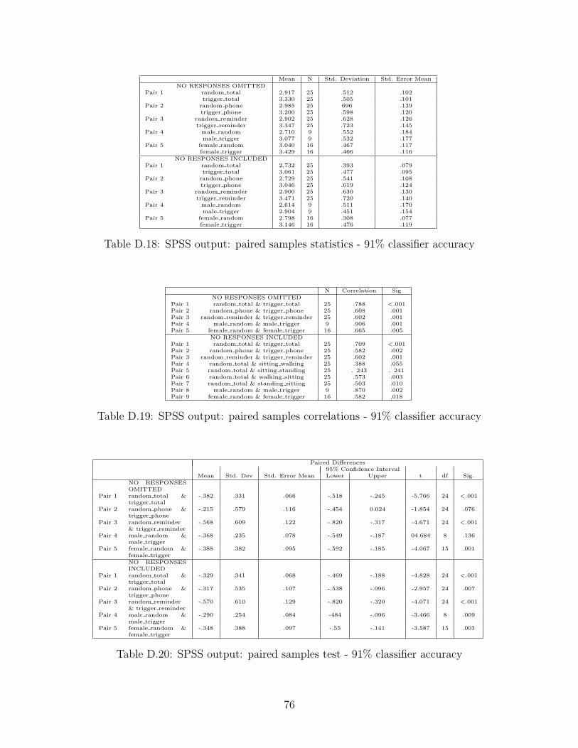
Mean N Std. Deviation Std. Error MeanNO RESPONSES OMITTED
Pair 1 random total 2.917 25 .512 .102trigger total 3.330 25 .505 .101
Pair 2 random phone 2.985 25 696 .139trigger phone 3.200 25 .598 .120
Pair 3 random reminder 2.902 25 .628 .126trigger reminder 3.347 25 .723 .145
Pair 4 male random 2.710 9 .552 .184male trigger 3.077 9 .532 .177
Pair 5 female random 3.040 16 .467 .117female trigger 3.429 16 .466 .116
NO RESPONSES INCLUDEDPair 1 random total 2,732 25 .393 .079
trigger total 3.061 25 .477 .095Pair 2 random phone 2.729 25 .541 .108
trigger phone 3.046 25 .619 .124Pair 3 random reminder 2.900 25 .630 .130
trigger reminder 3.471 25 .720 .140Pair 4 male random 2.614 9 .511 .170
male trigger 2.904 9 .451 .154Pair 5 female random 2.798 16 .308 .077
female trigger 3.146 16 .476 .119
Table D.18: SPSS output: paired samples statistics - 91% classifier accuracy
N Correlation SigNO RESPONSES OMITTED
Pair 1 random total & trigger total 25 .788 <.001Pair 2 random phone & trigger phone 25 .608 .001Pair 3 random reminder & trigger reminder 25 .602 .001Pair 4 male random & male trigger 9 .906 .001Pair 5 female random & female trigger 16 .665 .005
NO RESPONSES INCLUDEDPair 1 random total & trigger total 25 .709 <.001Pair 2 random phone & trigger phone 25 .582 .002Pair 3 random reminder & trigger reminder 25 .602 .001Pair 4 random total & sitting walking 25 .388 .055Pair 5 random total & sitting standing 25 . 243 . 241Pair 6 random total & walking sitting 25 .573 .003Pair 7 random total & standing sitting 25 .503 .010Pair 8 male random & male trigger 9 .870 .002Pair 9 female random & female trigger 16 .582 .018
Table D.19: SPSS output: paired samples correlations - 91% classifier accuracy
Paired Differences95% Confidence Interval
Mean Std. Dev Std. Error Mean Lower Upper t df Sig.NO RESPONSESOMITTED
Pair 1 random total &trigger total
-.382 .331 .066 -.518 -.245 -5.766 24 <.001
Pair 2 random phone &trigger phone
-.215 .579 .116 -.454 0.024 -1.854 24 .076
Pair 3 random reminder& trigger reminder
-.568 .609 .122 -.820 -.317 -4.671 24 <.001
Pair 4 male random &male trigger
-.368 .235 .078 -.549 -.187 04.684 8 .136
Pair 5 female random &female trigger
-.388 .382 .095 -.592 -.185 -4.067 15 .001
NO RESPONSESINCLUDED
Pair 1 random total &trigger total
-.329 .341 .068 -.469 -.188 -4.828 24 <.001
Pair 2 random phone &trigger phone
-.317 .535 .107 -.538 -.096 -2.957 24 .007
Pair 3 random reminder& trigger reminder
-.570 .610 .129 -.820 -.320 -4.071 24 <.001
Pair 4 male random &male trigger
-.290 .254 .084 -484 -.096 -3.466 8 .009
Pair 5 female random &female trigger
-.348 .388 .097 -.55 -.141 -3.587 15 .003
Table D.20: SPSS output: paired samples test - 91% classifier accuracy
76

Mean N Std. Deviation Std. Error MeanNO RESPONSES OMITTED
Pair 1 random total 2.939 25 .538 .108trigger total 3.306 25 .503 .101
Pair 2 random phone 2.911 25 742 .148trigger phone 3.294 25 .620 .124
Pair 3 random reminder 2.867 25 .799 .160trigger reminder 3.380 25 .740 .148
Pair 4 male random 2.713 9 .556 .185male trigger 3.065 9 .552 .184
Pair 5 female random 3.063 16 .497 .124female trigger 3.421 16 .448 .112
NO RESPONSES INCLUDEDPair 1 random total 2.767 25 .447 .089
trigger total 3.011 25 .510 .102Pair 2 random phone 2.694 25 .609 .122
trigger phone 3.076 25 .626 .125Pair 3 random reminder 2.791 25 .535 .107
trigger reminder 3.028 25 .797 .159Pair 4 male random 2.605 9 .514 .171
male trigger 2.922 9 . 576 . 192Pair 5 female random 2.846 16 . 390 . 098
female trigger 3.107 16 .442 .111
Table D.21: SPSS output: paired samples statistics - 82% classifier accuracy
N Correlation SigNO RESPONSES OMITTED
Pair 1 random total & trigger total 25 .702 <001Pair 2 random phone & trigger phone 25 .319 .120Pair 3 random reminder & trigger reminder 25 .427 .033Pair 4 male random & male trigger 9 .752 .019Pair 5 female random & female trigger 16 .575 .020
NO RESPONSES INCLUDEDPair 1 random total & trigger total 25 .587 .002Pair 2 random phone & trigger phone 25 .273 .186Pair 3 random reminder & trigger reminder 25 .548 .005Pair 4 male random & male trigger 9 .607 .083Pair 5 female random & female trigger 16 .525 .037
Table D.22: SPSS output: paired samples correlations - 82% classifier accuracy
95% Confidence IntervalMean Std. Dev Std. Error Mean Lower Upper t df Sig.
NO RESPONSESOMITTED
Pair 1 random total &trigger total
-.367 .403 .081 -.533 -.200 -4.550 24 <.001
Pair 2 random phone &trigger phone
-.383 .800 .160 -.713 -.053 -2.393 24 < .001
Pair 3 random reminder& trigger reminder
-.512 .826 .165 -.853 -.172 -3.103 24 .005
Pair 4 male random &male trigger
-.352 .390 .130 -.651 -.052 -2.708 8 .027
Pair 5 female random &female trigger
-.358 .438 .109 -.591 -.125 -3.271 15 .005
NO RESPONSESINCLUDED
Pair 1 random total &trigger total
-.245 .439 .088 -.426 -.064 -2.790 24 .010
Pair 2 random phone &trigger phone
-.381 .745 .149 -.669 -.074 -2.561 24 .017
Pair 3 random reminder& trigger reminder
-.237 .674 .135 -.515 -.042 -1.756 24 .092
Pair 4 male random &male trigger
-.317 .390 .130 -.651 -.052 -1.955 8 .086
Pair 5 female random &female trigger
-.261 .408 .102 -.479 -.044 -2.561 15 .022
Table D.23: SPSS output: paired samples test - 82% classifier accuracy
77

t-test because there were not enough data points. Table D.24 shows the breakdown of
the expected number of responses for each activity transition along with the standard
deviation. Even though sitting to walking and walking to sitting transitions had an
average of 4-6 responses per subject, the standard deviation was too large. Subjects
could have experienced only 1-2 interruptions for that particular type of activity
transition and answered the extreme cases on these interruptions (1 or 5), thereby
potentially skewing the result in one direction.
sit-walk sit-stand walk-sit stand-sitMean 5.92 1.96 4.6 1.71
Standard Deviation 2.75 1.86 2.87 1.78
Table D.24: The mean and standard deviation for the number of responses per activitytransition
78

Appendix E
Receiver Casing
All the details for building the receiver casing can be found in this section of the
Appendix. The casing utilizes the shape of the COMPAQ expansion sleeve without
the compact flash card. The receiver housing prevents the user from damaging the
receiver or the iPAQ connector. In addition, the casing was designed so that the user
would not find it awkward to carry the PDA.
E.1 Parts
The parts necessary for constructing the receiver casing can be found below. They
are separated by the parts necessary for the PDA sleeve, constructing the cable from
the receiver to the PDA, and the parts necessary to maintain power to the receiver.
Name Part Description Part Number Vendor QuantityPDA PARTS
Sleeve iPAQ Expansion Sleeve 3S562-001 services.foxconn.com 1Cover iPAQ Expansion Sleeve 3S569-001 services.foxconn.com 1Screw iPAQ Expansion Sleeve Screw 3S506-001 services.foxconn.com 2Screw iPAQ Expansion Sleeve Screw 3S507-001 services.foxconn.com 2
Connector Covering Casing for Connector Self-manufactured laser cut 1CABLE PARTS
Wire 4-wire cable NMUF 4/30-4046 SJ coonerwire 1Receiver Connector CONN SOCKET HOUSING 4POS 1.25 MM H2181-ND digikey 1
Crimp 26-30 AWG CRIMP TIN H9992CT-ND digikey 4PDA Connector iPAQ Connector ICP-21 gomadic 1POWER PARTS
Female Power Jack CONN DC PWR PLUG 0.7 x 2.355 MM CP-0120-ND digikey 1Male Power Jack CONN PWR JACK 0.65 x 2.75 MM SMT CP-023PJ-ND digikey 1
NiMH Gumstick Battery 1.2V 1350mAh NiMH Cell HF-A1U batteryprice 3Battery Charger WallMount 3 cell battery charger PST-5830-3 powerStream 1
Table E.1: iPAQ receiver casing parts
79

E.2 Pin-out Diagrams
All the necessary diagrams of the pin-outs have been provided below. Figure E-1
shows the description of the pinout of the connector on the iPAQ side. The pins used
by the receiver casing are 1-4, 7,8, 10, 14, and 22. There have been two different
types of the 22-pin iPAQ connector, the pin numbering for both types can be found
in Figure E-2. The pinout for the connector to the wireless receiver can be found in
Figure E-3.
Figure E-1: The 22-pin connections on the iPAQ connector side
The diagram for the power connector on the iPAQ side can be found in Figure E-4.
For the battery charger, the wire that is black and white is v+, while black is ground.
80
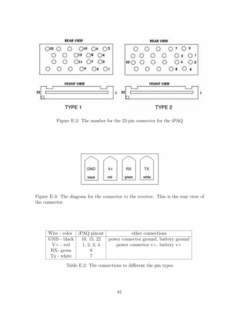
Figure E-2: The number for the 22-pin connector for the iPAQ
Figure E-3: The diagram for the connector to the receiver. This is the rear view ofthe connector.
Wire - color iPAQ pinout other connectionsGND - black 10, 15, 22 power connector ground, battery ground
V+ - red 1, 2, 3, 4 power connector v+, battery v+RX- green 8Tx - white 7
Table E.2: The connections to different the pin types
81

Figure E-4 shows how the wire attaches to the connector.
Figure E-4: Power connector to the housing of the connector on the iPAQ side andpower connection for the charger.
E.3 Instructions
The instructions for building the casing can be found below. They should be followed
in order to build the iPAQ casing efficiently.
E.3.1 Discharging and Charging the Batteries
Make sure to charge and discharge the batteries completely 2-3 times before connect-
ing them to the casing. It will help prolong the battery life. Solder 3 NiMH batteries
in serial, it is easiest to place them such that the ground of one battery is adjacent
to the v+ of the 2nd battery. The batteries should be taped together so that they
will not move around. To discharge the batteries, a circuit with 7 resistors of value
81 ohm should be connected in parallel. It will take approximately 4 hours to safely
discharge the batteries since each resistor can withstand up to 0.25 watts.
E.3.2 Connector Cable
A cable that connects the iPAQ connector to the wireless receiver needs to be man-
ufactured before any of the steps can be completed.
1. Strip the cable remove all the extra sheath until the 4 individual wires are
exposed.
2. Tin the 4 individual wires, making sure not to put too much solder on the wires.
82

3. Attach a crimp to each individual wire, making sure that there is not an excess
of solder to prevent proper crimping of the wire.
4. Crimp the sides using the plier so it will fit into the connector.
5. Place the wires into the connection using Figure E-2 as a reference for the
correct placement of each wire. The connector is inserted such that the latch
on the crimp touches the part of the connector hole that is curved.
6. Fit the connector into the wireless receiver to make sure that the connectors
stay in place and check the continuity using the receiver board. There should
be no shorts between any of the 4 wires.
7. Hot glue the connector so the connectors will not get pulled out or shorted with
each other. Figure E-5 is a picture of a completed cable.
Figure E-5: A completed wireless receiver cable to connect to the wireless receiver.
E.3.3 Building the Sleeve Cover
1. Sand down the interior of the sleeve cover so that the inside is flat.
2. Cut the foam to fit the inside cover.
3. Cut the battery shape, aligning the bottom of the battery pack to the edge of
the two bottom screw holes.
4. Cut the receiver shape, making sure that there is foam between the battery and
the receiver and between the receiver and the opening. Figure E-6 illustrates
the previous 4 steps.
83

5. Cut out sections for the tabs so that the cover will snap into the jacket easily.
Figure E-6: Starting from the left: a sanded interior of the cover, foam cut to fit theinside cover, and the finished cover
E.3.4 Preparing the Sleeve Jacket for the Connector
1. Drill the two holes to hold the connector in place using the template. Align the
template such that the top of the template is aligned to the edge of the jacket.
Figure E-7 illustrates the placement of the template. The hole should be drilled
using the eighth of an inch drill bit.
2. Place a connector into the housing and test to make sure the iPAQ slides in
easily. Adjust the holes until satisfactory.
3. Remove the template and drill the cable hole to the left of the right most hole.
Make sure to avoid drilling through the screw hole or the connector piece that
keeps the iPAQ in place. Figure E-8 shows the finished holes.
84
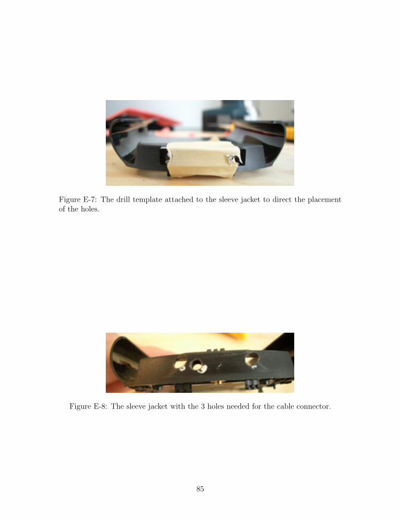
Figure E-7: The drill template attached to the sleeve jacket to direct the placementof the holes.
Figure E-8: The sleeve jacket with the 3 holes needed for the cable connector.
85

E.3.5 Connector Housing
The connector housing needs to be constructed using a laser cutter and black acrylic.
There are two types of acrylic used. The thin acrylic that will serve as the base of the
connector house needs to be countersinked so that the flathead screws will sink into
the housing and will not protrude in the base. The piece that will hold the connector
casing to the sleeve and the piece that will house the iPAQ connector needs to be
tapped with the appropriate tapping tool. Figure E-9 shows the 3 parts that need to
be tapped or sinked.
Figure E-9: The different parts of the connector housing that need to be tapped orcountersinked.
E.3.6 Wiring the Connectors
1. Determine pin number 1 using the diagram in Figure E-2, and mark it.
2. Sand or cutoff until the flat side of the connector fits into the housing.
3. String the cable through the necessary holes which is through the hole in the
sleeve jacket and the middle piece for the housing. Figure E-10 is a picture of
the completion of this step.
4. Solder the grounds together with wires, which are pins 10, 15, and 22. Tinning
the wire beforehand will help the connection.
86

Figure E-10: Stringing the cable through the necessary parts in order to create thehousing.
5. Solder an extra wire to the grounds that will connect to the power jack ground.
It needs to be long enough to go from the connector to the power jack (approx-
imately 1 inch).
6. Solder the ground from the wireless receiver cable to any of the 3 ground pins
on the iPAQ connector.
7. Solder all the voltage lines together (pins 1, 2, 3, 4) with wires. Include an extra
wire to run to the voltage of the power jack connector which is approximately
1 inch in length too.
8. Solder the voltage wire from the receiver to any of the 4 voltage pins on the
iPAQ connector.
9. Solder the RX and TX wires from the receiver to pins 7 and 8. The green wire
attaches to pin 8 and the white wire attaches to pin 7. Basically the RX on the
iPAQ needs to be connected to the TX on the wireless accelerometer.
87

10. Pull the cables through the left side of the connector, and connect the extra
ground and voltage wires to the connector. See the pinout diagram shown in
Figure E-4.
11. Solder another extra set of wires (ground and voltage) that will tie the batteries
to the power connector. The wires need to be long enough to run through the
cable hole to the batteries on the cover. Pull the wires through the cable hole.
12. Test to make sure voltage and ground are not shorted together. This is impor-
tant as there is high current from the battery.
13. Screw together the connector casing, making sure not to screw too tightly oth-
erwise the acrylic will break. Figure E-11 shows the steps to place the housing
together. Figure E-12 for a picture of a completed connector housing.
Figure E-11: The process of putting the housing for the connectors together in aclockwise manner.
14. Connect the battery to the wires to the power jack.
15. Plug in the receiver and make sure there is a connection to all the proper pins
and also test to make sure the iPAQ can read data from the receiver.
16. Remove the coin battery holders from the back of the wireless receiver, and
replace with wires. See Figure E-13 for a picture of the modified receiver.
88
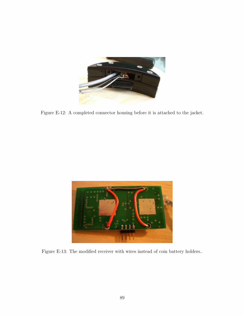
Figure E-12: A completed connector housing before it is attached to the jacket.
Figure E-13: The modified receiver with wires instead of coin battery holders..
89

17. Attach the casing to the sleeve using screws.
18. Strip off the original connector on the charger and replace with the male power
plug. Using Figure E-4 as the guide, connect the wire that is black and white
to voltage, and black to the ground pin.
19. Check to make sure the charger works with the batteries.
20. Close the cover and the jacket, and place the proper sleeve screws to keep the
cover in its place.
90

Appendix F
Experiment Graphical User
Interface Screenshots
The user interface for the interruption study was based on the Context Aware Expe-
rience Sampling (CAES) design [21]. Minor modifications were made to the screens.
Additionally, the screen flow was simplifed to shorten the user-iPAQ interaction time.
The screen flow and the screen interface are described below.
F.1 Screen Flow
There are 3 main screens that the user could experience during the study: the start
screen, the question screen, and the mute screen. Figure F-1 illustrates the user-iPAQ
interaction. The arrows shows how the screens were linked to each other.
The user entered the mute screen from the start screen by pressing the mute
button. Once the mute screen was displayed, it returned to the start screen when
the user chose an amount of time to mute the study, if s/he decided against muting
the study, or if the user has spent more than one minute on the screen. The question
screen appeared when a question had been triggered (either randomly or by an activity
transition). Once the user answered the question, or if the user has not responded
within one minute, the start screen was restored.
91

Figure F-1: A flow chart for the interaction between the user and the PDA
F.2 Screen Interface
The default screen contained information relevant to the user. The main purpose of
the screen was to allow the user to mute the study. The screen also contained the
time of day, the researcher’s contact information, and the current status of the study.
During the experiment, two different entries were used for the status screen: “Status
OK” or “Call Joyce Please”. The user was notified to call the researcher if there were
problems with the accelerometer data. The screen shot can be found in Figure F-2.
The user had the option of muting the study although users were informed not
to use mute unless absolutely necessary. The audio sounds were designed to slowly
increase in volume so that it would not be too distracting to others. Subjects were
not penalized for using the mute button. They had the option to mute the study up
to a maximum of one hour. Any time above one hour would lead to a considerable
loss of interruptions experienced by the subject.
The question screen was designed to limit the amount of text the user had to
read. An icon that represented the question was used along with a short phrase
to remind the subject of the question. The interface is shown in Figure F-3. The
92

Figure F-2: The start screen and the mute screen for the experiment.
two questions the user experienced were: “How receptive are you to a phone call?”
or “How receptive are you to a reminder?” The screen chose a question to ask at
random. When the user tapped on the screen, the auditory signal stopped. The
interface captured the amount of time it took the user to tap the screen, and the
elapsed time between tapping the screen and pressing the OK button.
93

Figure F-3: The question screen associated with the question ”How receptive are youto a phone call?”
94

Appendix G
Feature Calculation and Decision
Tree Algorithm
This section contains the details of the activity detection algorithm.
G.1 Feature Calculation
Mean, energy, entropy, and correlation features are calculated for each accelerometer.
In order to extract the features from the sampling window, the raw accelerometer
data needs to be run through a discrete Fast Fourier Transform (FFT). Since the
accelerometer data were all real numbers, a real-valued FFT was used. This saved
computation time over a standard complex-valued FFT. The sampling window was
used during the process of calculating the FFT of the accelerometer data. Once the
raw accelerometer data was transformed into the frequency domain using an FFT,
each data point was a complex number, containing a real and imaginary component.
For the purpose of understanding the formulas, Equation G.1 contains the notation
used in this appendix. In addition, n represents the sampling window used and the
subscript j represents the jth data point of the window.
x = a + b ∗ i, x = complex, a = real, b = imaginary (G.1)
95

The first set of features extracted from the sampling window was the mean for
each axis. The mean represents the DC component over the entire window. The mean
feature was not used in the classifier, but might be used in future classifications. The
formula for the mean can be found in Equation G.2.
mean =n∑
j=1
aj
n(G.2)
The energy of each axis is the sum of the squared component magnitudes normal-
ized by the window size. This calculates the energy of the signal over the sampling
window of each axis. Equation G.3 contains the mathematical representation for the
energy of an axis.
energy =n∑
j=1
a2j + b2
j
n(G.3)
The entropy is calculated using the normalized information entropy of the discrete
FFT component magnitudes of the signal. This feature helps differentiate between
two activites that may have same energy values but different patterns of movement.
A nearly uniform movement will have a lower frequency-domain entropy value in
comparison to a jerky movement. The entropy is calculated using Equation G.4
entropy =n∑
j=1
cj ∗ log(cj), cj =
√a2
j + b2j∑n
k=1
√a2
k + b2k
(G.4)
Finally, the correlation between two axes of acceleration for the sampling window
is calculated by taking the dot product of the two axes normalized over the window
size. The formula for this computation is in Equation G.5. Let a represent the real
part of axis 1 and c represent the real part of axis 2.
correlation =n∑
j=1
aj × cj (G.5)
The correlation was calculated between each of the three different axes for each ac-
celerometer but was not computed between axes on different accelerometers to save
96

processing time. Instead, the decision tree indirectly computes the correlation be-
tween axes on different accelerometers using the energy of the different axes on sep-
arate accelerometers. This saves computation time since feature calculation is more
costly than traversing the decision tree. Future algorithms could utilize the correlation
between accelerometers to improve the trained C4.5 supervised learning classifier.
G.2 Decision Tree Algorithm
The decision tree was trained using WEKA software [30]. The C4.5 classifier was
trained using 10 different subjects [20]. Each type of activity has approximately 1500
training cases, or 150 cases per subject. The training data was formatted into a text
file that was saved in the format specified by the WEKA software. A sample of the
WEKA format can be found in Figure G-1. After loading the file, the J48 decision tree
was used on the training data set. WEKA built a decision tree using the training cases.
The tree was saved into a result buffer and loaded onto the iPAQ. The file is located
on the iPAQ in the location: \iPAQ File Store\Interruption\config\wekaTree.txt.
The real-time classifier parses the decision tree and computes all the necessary
nodes to classify incoming data. A sample decision tree can be see in Figure G-2.
The algorithm classifies a window using the sample decision tree in the following
manner:
1. Is the z-entropy of accelerometer 2 less than or equal -0.835391? If the outcome
is true, then the activity associated with this sampling window is walking. If
not, proceed onto the next step.
2. Is the correlation between the y-axis and the z-axis of accelerometer 2 less than
or equal to a certain value? If it is, then proceed to step 3. Otherwise, skip to
step 6.
3. Is the correlation between the x-axis and and the y-axis of accelerometer 1 less
than or equal to 16564758768? If it is, proceed to the next step. Otherwise,
skip to step 5.
97

Figure G-1: A sample of the WEKA file format for training a new classifier.
98

Figure G-2: A sample decision tree built by WEKA.
4. Is the x-entropy of accelerometer 1 less than or equal to -0.389781? If it is, then
the activity is standing. If the outcome is false, then it is sitting.
5. Is the correlation between the x-axis and z-axis greater than 16564758768 ? If
it is, then the activity of this window is sitting.
6. Is the correlation between the y-axis and z-axis greater than a certain value?
If the result is yes, then the activity associated with this sampling window is
standing.
In addition, any changes to the sampling window will not affect the manner in
which the features are calculated and classified. However, the real-time activity clas-
sifier must have been trained using features with the same sampling window. If the
classifier was trained on a different window, the detection accuracy may decrease
drastically.
Each time new features were calculated for the sampling window, the algorithm
would classify the window using these extracted features. The decision tree used
for the study contained 49 nodes with 25 leaves and took 1.94 seconds to build on
a 3GHz Pentium 4 computer. The tree was learned from the training set, but it
can be interpreted with visual insepction. The algorithm first checks the amount
99

of movement of the ankle accelerometer. The classifier then checks the orientation
of the second accelerometer, and then breaks off to test the correlation between the
different axes on separate accelerometers by comparing the energy of the axes.
The lag time between the activity and the classification results from the following
computations:
data acquisition + FFT calculation + features computation
+decision tree classification time = total lag time
For the interruption study, the algorithm took between 3-5 seconds from the time
of the activity occurrence to detection of the activity. The lag time is not constant
because the activity may not have been captured in the features of the first sampling
window. As a result, the algorithm might not detect the activity until the second
sampling window which is 1.28 seconds later.
100

Appendix H
Training a Classifier
This section contains the instructions for training a new classifier. There are four
different aspects of the classifier that need to be determined: the sampling window,
the number of accelerometers to use, the type of activities, and the number of cases
per activity. This section outlines the considerations that need to be taken when
deciding on the four aspects. The last portion of this section discusses modifications
needed to make to the program that was built to collect training data.
H.1 Sampling Window
A smaller sampling window will result in a more responsive classifier since it takes less
time to compute the transform and extract the features. However, a small window
also limits the number of activities that the classifier will be able to differentiate.
A larger window also has its pitfalls. It requires more memory and has a longer
processing time. Currently, the algorithm uses a sampling window of 256 points (or
2.56 seconds) and an overlapping window of 128 samples (or 1.28 seconds). Finally,
the window must be a power of 2 (256 = 28) in order to compute the FFT.
101

H.2 Number of Accelerometers
The number of accelerometers used determines the sampling rate of each accelerome-
ter because the wireless receiver has a maximum sampling frequency of 200 Hz regard-
less of the number of accelerometers used. The sampling rate for each accelerometer
can be calculated by taking 200 Hz and dividing by the number of accelerometers.
The algorithm currently uses 2 accelerometers and therefore has a sampling rate of
100 Hz per accelerometer.
H.3 Type of Activities
The range of activities that can be detected is dependent upon the number and place-
ment of the accelerometers used. The list of activities that can be currently recognized
along with the number, placement and sampling frequency of the accelerometers is
summarized in Appendix C of Bao’s work [2]. The number of activities can also af-
fect the computation time necessary to classify a sampling window. An increase in
recognition activities can result in a larger decision tree, requiring a longer period of
time to traverse the tree.
H.4 Number of Training Cases
The number of training examples available will affect the accuracy of the decision tree.
A larger training data set may result in a more accurate model, but could also lead
to a complex decision tree with an abundance of nodes. However, a small training
set may not necessarily encapsulate the general population and might thereby result
in a poor performance in detection accuracy for certain users.
H.5 Obtaining Training Data
The program that has been built to collect training data can be found in the following
location: ActivityDetection\Software\GatherActivityData. The code will need to be
102

changed to account for the sampling window, the types of activities, the number of
accelerometers, and the number of training cases per subject. Currently the software
will only gather data for a maximum of 2 accelerometers, but it can be easily mod-
ified to incorporate up to 6 accelerometers. The sampling window and overlapping
window are adjusted by changing the number associated with the definition of the
FFT WINDOW and FFT OVERLAP. The types of activities can be loaded into the
array containing the strings for all possible activities. Finally, the number of training
cases per subject is determined by the amount of time the program spends gathering
data for each type. A longer duration between activities leads to a larger number of
cases per subject.
Once the modified software has been deployed onto an iPAQ, the user training the
algorithm wears the sensors and performs the activity that is written on the iPAQ
screens. The user is prompted of a change in activity with a beep. When the software
has finished gathering all the training data for this particular user, the researcher
uncompresses the feature file into a comma-delimited format. The program can be
found under DataCollection\Software\FeatureLogConverter. Two steps are needed
before transferring the data into the WEKA training file format. The data between
activity transitions are removed since they may not be correctly classified. This is
done by removing the 5 samples before a new activity occurred and the 5 samples
after a new activity occurred. Finally, the researcher needs to fill in the string for the
appropriate activity since the activities is referenced by numbers in the feature file.
Upon completion of the two steps, the feature file is copied into the WEKA training
file. Each subject has his/her own feature file, and the WEKA training file contains
the data for all features. The WEKA file is then be loaded in the WEKA software
and be used to generate a decision tree.
103

104

Appendix I
Statistical Analysis
This section describes the details for analyzing the subjects’ responses. The responses
were aggregated on the subject level using the method described in the first portion
of this appendix. The aggregated data was then analyzed using SPSS, a statistical
analysis program.
I.1 Aggregating the Data on the Subject Level
The subject’s responses were loaded into three separate Excel files. One excel file
performed the analysis on the actual experiment data. The second Excel file was
used to simulate the average classifier scenario. 9% of the triggered responses for each
subject were selected randomly and converted to random interruption responses. The
final Excel file was used to simulate the worst case scenario in which the classifier
performed one standard deviation below the average. Instead of selecting 9% of the
triggered responses, 18% of the triggered responses were moved to random responses.
There are two sets of calculations that are computed for all three excel files. For the
first set of calculations, the “no responses ” were omitted. Figure I-1 illustrates this
first set of sorted calculations.
The first set of calculations involves taking the mean and standard deviation of
the following:
1. All random triggered responses
105

Figure I-1: A sorted subject response with all the no responses omitted.
106

2. All activity transition triggered responses
3. Random triggered responses for the phone call
4. Activity transition triggered responses for the phone call
5. Random triggered responses for the reminder
6. Activity transition triggered responses for the reminder
The second set of calculations requires sorting by the trigger type without omitting
the “no responses.” Instead, the “no responses” were assumed to be situations where
the subject answered a 1. The mean and standard deviation were recalculated for all
random triggered responses and all activity transition triggered responses.
The individual activity transitions were not analyzed because there were not
enough data points for each transition per subject. Refer to Appendix D for the
discussion of the exclusion of these transitions in the analysis.
I.2 Measuring Statistical Significance
After aggregating the data on the subject level, all the data need to be entered into
a statistical analysis program. Figure I-2 shows a sample of the program used to
analyze the significance of the data. A two-tailed paired t-test is used to determine
if two population means are equal when the data is dependent (a within-subjects
design). The following paired t-tests were used to determine the significance of the
results with the no responses omitted.
1. All random responses to all activity transition triggered responses
2. Random responses for the phone call to the activity transition triggered re-
sponses for phone call
3. Random responses for the reminder to the activity transition triggered responses
for the reminder
107

Figure I-2: The aggregated subject data entered in a statistical analysis program.
4. All random responses to the responses for sitting to walking
5. All random responses to the responses for sitting to standing
6. All random responses to the responses for walking to sitting
7. All random responses to the responses for standing to sitting
8. Random responses to all activity transition triggered responses for males
9. Random responses to all activity transition triggered responses for females
A paired t-test was also used to compare all random responses to all activity transition
triggered responses with the no responses taken into account. No responses were
assumed to be equivalent to a 1, which is lower than not at all receptive.
A 95% confidence level was used for the paired t-tests. In addition, the significance
level was established at p =0.05. Following convention, in this work any t-test with an
associated p <0.05s is considered to be statistically significant. Appendix D contains
the descriptions for the output of a statistical analysis program.
108

The possible problems with this method is that it does not account for the differ-
ence in number of interruptions experienced. A subject that experienced interruptions
more frequently might have a lower difference in mean as opposed to a subject that
experienced sporadic interruptions. However, the paired t-test does not consider this
factor and places equal weight on both differences in mean. Another potential prob-
lem with the paired t-test is the need to aggregate the data on the subject level. The
mean of the mean of each subject is used to represent the overall response of the
subject. This does not take into account the variances in responses. A large variance
in a subject’s response might change the significance level of the results because the
responses did not converge to a value, so the mean could actually not be a useful
representation of the subject’s overall receptivity.
109

110

Appendix J
Data Availability for Other
Researchers
The data collected for this work is available without cost to the public for research pur-
poses. Contact Stephen Intille at [email protected] for information regarding acquiring
the data. The data set includes raw accelerometer data, interruption study responses,
trained C4.5 supervised learning classifier, chime sound file, post-experiment inter-
views, and a summary of the demographic data. The data set has been compressed
to size of 300 MB. The format of the data set can be found in Appendix C.
111

112

Bibliography
[1] B. P. Bailey, J. A. Konstan, and J. V. Carlis. Measuring the effects of interrup-
tions on task performance in the user interface. In IEEE Conference on Systems,
Man, and Cybernetics 2000 (SMC 2000), pages 757–762. IEEE Press, 2000.
[2] L. Bao. Physical Activity Recognition from Acceleration Data under Semi-
Naturalistic Conditions. M.Eng. Thesis, Massachusetts Institute of Technology,
2003.
[3] L. Bao and S.S. Intille. Activity recognition from user-annotated acceleration
data. In A. Ferscha and F. Mattern, editors, Proceedings of PERVASIVE 2004,
volume LNCS 3001, pages 1–17. Springer-Verlag, Berlin Heidelberg, 2004.
[4] E. Cutrell, M. Czerwinski, and E. Horvitz. Effects of instant messaging interrup-
tions on computing tasks. In Extended Abstracts of CHI 2000, Human Factors
in Computing Systems, pages 99–100. ACM Press, 2000.
[5] T. Gillie and D. Broadbent. What makes interruptions disruptive? A study of
length, similarity, and complexity. Psychological Research, 50(4):243–50, 1989.
[6] S.M. Hess and M. Detweiler. Training to reduce the disruptive effects of inter-
ruptions. In Proceedings of the HFES 38th Annual Meeting, volume 2, pages
1173–1177. 1994.
[7] K. Hinckley and E. Horvitz. Toward more sensitive mobile phones. In Proceedings
of the 14th annual ACM Symposium on User Interface Software and Technology,
pages 191–192. ACM Press, 2001.
113

[8] E. Horvitz and J. Apacible. Learning and reasoning about interruption. In Pro-
ceedings of ICMI 2003: ACM International Conference on Multimodal Interfaces,
pages 20–27. ACM Press, 2003.
[9] E. Horvitz, A. Jacobs, and D. Hovel. Attention-sensitive alerting. In Proceedings
of UAI ’99, Conference on Uncertainty and Artificial Intelligence, pages 305–513.
Morgan Kaufmann, 1999.
[10] E. Horvitz, C.M. Kadie, T Paek, and D. Hovel. Models of attention in computing
and communications: From principles to applications. Communications of the
ACM, 46(3):52–59, 2003.
[11] E. Horvitz, P. Koch, C. Kadie, and A.. Jacobs. Coordinates: Probabilistic fore-
casting of presence and availability. In Proceedings of the 18th Annual Conference
on Uncertainty in Artificial Intelligence (UAI-02), pages 224–233. Morgan Kauf-
mann Publishers, 2002.
[12] James M. Hudson, Jim Christensen, Wendy A. Kellogg, and Thomas Erickson.
“I’d be overwhelmed, but it’s just one more thing to do”: Availability and inter-
ruption in research management. In Proceedings of the Confererence on Human
Factors in Computing Systems, pages 97–104. ACM Press, 2002.
[13] S.E. Hudson, J. Fogarty, C.G. Atkeson, D. Avrahami, J. Forlizzi, S. Kiesler, J.C.
Lee, and J. Yang. Predicting human interruptability with sensors: A Wizard of
Oz feasibility study. In Proceedings of the Conference on Human Factors and
Computing, pages 257–264. ACM Press, 2003.
[14] N. Kern and B. Schiele. Context-aware notification for wearable computing. In
Proceedings of the 7th International Symposium on Wearable Computing, pages
223–230. IEEE Computer Society Press, New York, USA, 2003.
[15] K. K. Liu. A Personal, Mobile System for Understanding Stress and Interrup-
tions. S.M. thesis, Massachusetts Institute of Technology, 2004.
114

[16] P. Lukowicz, H. Junker, M. Staeger, T. von Bueren, and G. Troester. Wearnet: A
distributed multi-sensor system for context aware wearables. In UbiComp 2002:
Proceedings of the 4th International Conference on Ubiquitous Computing, pages
361–370. Springer: Lecture Notes in Computer Science, September 2002.
[17] C. E. McCarthy and M. E. Pollack. A plan-based personalized cognitive orthotic.
In Malik Ghallab, Joachim Hertzberg, and Paolo Traverso, editors, Proceedings
of the Sixth International Conference on Artificial Intelligence Planning Systems,
pages 243–252. AAAI Press, 2002.
[18] D. S. McCrickard and C.M Chewar. Attuning notification design to user goals
and attention costs. Communications of the ACM, 45(3):67–72, 2003.
[19] D.C. McFarlane. Coordinating the interruption of people in human-computer
interaction. In A. Sasse and C. Johnson, editors, Human-Computer Interaction
- INTERACT’99, pages 295–303. IOS Press, 1999.
[20] J. R. Quinlan. C4.5 : Programs for Machine Learning. The Morgan Kaufmann
series in machine learning. Morgan Kaufmann Publishers, San Mateo, CA, 1993.
J. Ross Quinlan. ill. ; 25 cm.
[21] J. Rondoni. A Context-Aware Application for Experience Sampling and Machine
Learning. M.eng. thesis, Massachusetts Institute of Technology, 2003.
[22] D. P. Siewiorek, A. Smailagic, J. Furukawa, A. Krause, N. Moraveji, K. Reiger,
J. Shaffer, and F. L. Wong. Sensay: A context-aware mobile phone. In 7th IEEE
International Symposium on Wearable Computers, pages 248–249, White Plains,
NY, 2003.
[23] C. Speier, J. S. Valacich, and I. Vessey. The effects of task interruption and
information presentation on individual decision making. In Proceedings of the
Eighteenth International Conference on Information Systems, pages 21–36. As-
sociation for Information Systems, 1997.
115

[24] A.A. Stone and S. Shiffman. Capturing momentary, self-report data: A proposal
for reporting guidelines. Annals of Behavioral Medicine, 24(3):236–243, 2002.
361.
[25] N. A. Storch. Does the user interface make interruptions disruptive? A study
of interface style and form of interruption (UCRL-JC-108993). Springfield:
Lawrence Livermore National Laboratory, 1992.
[26] A. Stouffs. Interruptions as multimodal outputs: Which are the less disrup-
tive? In Proceedings of the 4th IEEE International Conference on Multimodal
Interfaces, page 479. IEEE Computer Society, 2002.
[27] E. M. Tapia, N Marmasse, S. S. Intille, and K Larson. MITes: Wireless Portable
Sensors for Studying Behavior. In Extended Abstracts at The Sixth International
Conference of Ubiquitous Computing. 2004.
[28] M. van Dantzich, D. Robbins, E. Horvitz, and M. Czerwinski. Scope: Providing
awareness of multiple notifications at a glance. In Proceedings of AVI 2002, ACM
Conference on Advanced Visual Interfaces. ACM Press, 2002.
[29] R. van Solingen, E. Berghout, and F. van Latum. Interrupts: Just a minute
never is. IEEE Software, 15(5):97–103, 1998.
[30] I.H. Witten and E. Frank. Data Mining: Practical Machine Learning Tools and
Techniques with Java Implementations. Morgan Kaufmann, 1999.
116