International Journal of Heat and Mass Transfer 90 (2015) 1232–1240

Contents lists available at ScienceDirect

International Journal of Heat and Mass Transfer

journal homepage: www.elsevier .com/locate / i jhmt

An iterative, analytical method for solving conjugate heat transferproblems

http://dx.doi.org/10.1016/j.ijheatmasstransfer.2015.07.0560017-9310/� 2015 Elsevier Ltd. All rights reserved.

⇑ Corresponding author at: 500 W First St, Rm 211, Arlington, TX 76019, USA.Tel.: +1 (817) 272 9338; fax: +1 (817) 272 2952.

E-mail address: jaina@uta.edu (A. Jain).

Krishna Shah, Ankur Jain ⇑Mechanical and Aerospace Engineering Department, University of Texas at Arlington, USA

a r t i c l e i n f o

Article history:Received 16 April 2015Received in revised form 11 July 2015Accepted 11 July 2015

Keywords:Conjugate heat transferThermal conductionConvectionAnalytical methods

a b s t r a c t

Conjugate heat transfer involving convection and conduction in a fluid flow and a solid body in contactwith each other occurs commonly in engineering applications. While analytical solutions for individualconvection and conduction problems are relatively easier, it is a lot more challenging to solve thecombined conjugate heat transfer problem. In this paper, an iterative method is developed foranalytically solving conjugate heat transfer problems. Based on an initial assumption of the temperaturefield at the solid–fluid interface, the temperature distributions in the fluid and solid body are determinedby separately solving the governing energy conservation equations in the two domains. These solutionsare used to improve the initial assumption of the interface temperature until convergence. It is found thatonly a few iterations of this process are needed for convergence. Temperature fields computed from thisanalytical approach are found to be in good agreement with finite element simulation results. The iter-ative analytical approach is used to solve two technologically relevant problems related to internal andexternal flows. Given the general nature of the iterative approach, results from this paper may be helpfulin solving a variety of conjugate heat transfer problems.

� 2015 Elsevier Ltd. All rights reserved.

1. Introduction

Conjugate heat transfer involving coupled conduction andconvection is of significance in many engineering systems. A largevolume of past research [1–14] has been devoted to solving tem-perature fields for a fluid flowing in contact with a solid body,wherein thermal convection within the fluid domain occurs in con-junction with conduction within the solid domain. While the effectof conduction in the solid body is important in the thermallydeveloping fluid region [2,15], it is also clearly important in caseof internal heat generation in the solid that is being convected bythe flowing fluid [16]. This makes it critical to develop analyticalsolutions for conjugate problems involving convection in fluid flowand conduction in a solid which is in contact with the fluid flow.Problems involving external flow and internal flow are both ofinterest.

Derivation of solutions for convection-only or conduction-onlyproblems is relatively straightforward. Well-known solutions existfor specific boundary conditions such as constant temperature orconstant heat flux [1,4,5]. Similarly, theoretical solutions for a vari-ety of conductions problems are also available [17,18]. However,

analytical derivation of temperature distribution in conjugateproblems is in general a lot more challenging [19]. A fundamentalproblem underlying several conjugate heat transfer problems wasfirst solved by Graetz [3,4] who derived an analytical expressionfor temperature in a fluid flowing through a duct with constanttemperature boundary condition, assuming that the flow is hydro-dynamically developed and thermally developing. Analyticalexpressions for eigenvalues and eigenfunctions for this solutionhave been computed [7], and this solution has been used to derivethe solution for a more general problem with continuously or dis-cretely varying wall temperature using linear superimposition[2,7,8]. Boundary layer solution for fluid flow over a plate for ther-mal boundary layer nonsimilarity arising from both velocity fieldand streamwise variation of temperature have been analyzed [6].The case of constant or axially varying wall heat flux has also beenanalyzed. While axial conduction in the fluid is mostly neglected,some papers have accounted for this phenomenon [9,20], whichis relevant for specific technological applications.

While the classical convection problems for internal and exter-nal flows do not consider thermal conduction within the solid bodyin contact with the fluid flow, solutions to these problems providethe basic building block for deriving temperature distributions inconjugate problems where thermal conduction in the solid andthermal convection in the fluid must be considered

Nomenclature

a thermal diffusivityh convective heat transfer coefficientH height/thicknessk thermal conductivityL length of the platePr Prandtl numberq heat fluxQ volumetric heat generation rateR radiusRe Reynolds numberT temperatureu velocity

Subscripts0 initial valuee entryf fluidi innero outers solidr radial coordinatez axial coordinate1 freestream value

Superscript+ non-dimensional variable

Fig. 1. Schematic of a general conjugate heat transfer problem involving a fluid flowover an arbitrarily shaped solid with internal heat generation.

K. Shah, A. Jain / International Journal of Heat and Mass Transfer 90 (2015) 1232–1240 1233

simultaneously. A number of approaches have been presented forsolving this conjugate problem. A series form of the wall tempera-ture has been assumed, and energy conservation at the solid–fluidinterface has been used to derive expressions for coefficients of theseries form [10,11,21], resulting in analytical expressions for theentire temperature distribution. In particular, expressions for pipeflow [10], a plate in liquid or gas flow [11,12], flow betweenparallel plates [22,23] and for turbulent flows [20] have beenpresented. A solution for the conjugate problem of flow over a flatplate has also been presented using the method of the asymptoticsolution of singular integral equations [13]. In addition tosuch approaches, the integral transform technique has also beenused for solving conjugated heat transfer problems [24,25].Semi-analytical [26–30] and purely numerical [31–33] techniqueshave also been used. These papers utilize discretization based onfinite-element or finite-difference based methods.

This paper presents a solution for the conjugate heat transferproblem using an iterative approach that utilizes analytical solu-tions of both conduction and convection problems solved indepen-dently. Solutions to these two sub-problems are coupled with eachother through temperature continuity and energy conservation atthe solid–fluid interface. Both internal and external flow problemsare addressed. In this method, the temperature at the solid–fluidinterface is assumed, based on which the temperature distributionin the fluid is determined analytically. Using energy conservationat the interface, the solid temperature distribution is then deter-mined. The interface temperature determined from here is usediteratively to improve the wall temperature distribution until rea-sonable convergence. Such an approach has been used in the pastfor analytical determination of temperature distribution in thermalconduction problems in a multi-layer solid body [34–36]. In addi-tion, a few papers have also utilized a similar iterative method forsemi-analytical solution of conjugate heat transfer problems,wherein a finite-element or finite-difference discretizationapproach is used to numerically solve the thermal conductionproblem [26,28–30]. The present approach which determines bothfluid and solid temperature distributions analytically, results inreduced mathematical complexity compared to classical,non-iterative approaches [10–12,20,24], without the need to resortto discretization and numerical techniques used in pastsemi-analytical approaches [26–30]. It is found that only a smallnumber of iterations are sufficient for reasonable convergence ofresults. The iterative method is utilized to model conjugate heattransfer in two specific problems – the cooling of a hollow heatgenerating cylinder with anisotropic thermal conductivity, andthe cooling of a heat generating solid block due to fluid flow over

the block. These models represent technologically importantenergy conversion processes, for example, the liquid cooling ofan annular Li-ion cell [16] during a high-rate discharge process[37]. The next section presents the general iterative approach,followed by derivation of specific solutions for internal andexternal flow problems.

2. General solution: the iterative approach

This section presents the general approach for analytically solv-ing a conjugate problem involving thermal conduction and convec-tion in a solid and fluid flow respectively. Consider a solid (S) withan arbitrary shape as shown in Fig. 1. Fluid flow (F) occurs with agiven velocity profile. The solid and fluid intersect at an interface,denoted by S-F. In general, internal heat generation within thesolid is considered. Although Fig. 1 shows an external flow scenar-io, in general, fluid flow may occur either over the solid (externalflow), or through the solid (internal flow).

In general, the interest is in deriving expressions for tempera-ture distributions Ts (�x) and Tf (�x) where �x is the general spatial

1234 K. Shah, A. Jain / International Journal of Heat and Mass Transfer 90 (2015) 1232–1240

coordinate. Only the laminar, steady state problem is consideredhere. The governing conservation equations that must be solvedto determine these temperature distributions are given by

ar2Tf ¼ ð~v � rÞTf þ l �Uþ �gf ð1Þ

and

kr2Ts þ gsð�xÞ ¼ 0 ð2Þ

Here, l �U is the viscous dissipation, and �gf and �gs are volumet-ric heat generation rates in the solid and fluid respectively. Themethodology discussed in this paper for deriving analytical solu-tions for the temperature fields in S and F is based on analyticallysolving the temperature fields individually in the solid and fluiddomains, and utilizing principles of temperature compatibilityand conservation of energy at the interface to iterate until a stablesolution is obtained. To start with, the fluid temperature distribu-tion at the interface S-F is assumed to be

Tf ð�xS�FÞ ¼ T0ð�xS�FÞ ð3Þ

Assuming the velocity field in the fluid is known in advance,Eq. (1) can now be solved along with the assumed boundarycondition at the interface. Once Tf (�x) is known, the heat flux intothe solid at the solid–fluid interface can be obtained bydifferentiating.

qs;inð�xÞ ¼ kf@Tf

@�nð4Þ

where �n is the outward normal to the solid surface at the S-F.Eq. (4) represents a boundary condition for the temperature dis-

tribution in the solid Ts (�x). The governing equation (2) can now besolved along with Eq. (4). The solution for Ts (�x) provides a meansto determine the temperature of the solid at the interface, whichcan then be used to update the interface temperature distributionthat was assumed in Eq. (3). The entire procedure can be repeatedto determine the temperature distributions over multiple itera-tions. Eventually, the temperature distributions may be expectedto converge, with negligible change from one iteration to the next.

The analytical framework described above is used for analyzingboth internal and external flows, which are discussed in subse-quent sub-sections.

2.1. Internal flow

Consider the laminar flow of a fluid through an annular cylin-der, shown schematically in Fig. 2(a). The fluid flow is assumedto be hydrodynamically fully developed when it enters the cylin-der, with a given velocity profile u(r+) and entry temperature Te

at the entrance, z+ = 0. The solid portion of the cylinder is assumedto generate heat with a volumetric rate of Q. Convective heat trans-fer with coefficients hro and hz are assumed over the outer surfaceand axial faces of the cylinder respectively.

This general solid–fluid problem is commonly encountered inengineering applications, for example, in flow of a cold fluidthrough a Li-ion cell that generates heat due to electrochemicalenergy conversion within the cell [16,37]. The interest in is deriv-ing expressions for cell and coolant temperature fields due to aspecific internal heat generation rate and coolant flowrate.

To start with, a temperature distribution is assumed at the wall

Tf ðzþ; rþ ¼ 1Þ ¼ TwallðzþÞ ¼ T0ðzþÞ ð5Þ

Neglecting viscous dissipation, heat transfer in the fluid domainis governed by the following governing conservation equation [1],

@2Tþf@rþ2 þ

1rþ

@Tþf@rþ¼ ð1� rþ2Þ

@Tþf@zþ

ð6Þ

The non-dimensional coordinates z+ and r+ are given by

zþ ¼ z=Ri

Re � Prð7Þ

rþ ¼ rRi

ð8Þ

and temperature is non-dimensionalized as follows:

Tþf ¼Tf

QH2=kr

ð9Þ

The temperature solution based on a given Tþf (z+, r+ = 1) isobtained as follows [1]

Tþf ðzþ; rþÞ � Tþe ¼Z xþ

0½1� hðzþ � nþ; rþÞ� dTþwallðn

þÞdnþ

dnþ

þXk

i¼1

1� hðzþ � nþi ; rþÞ

� �Tþwallðn

þi Þ � Tþe

� �ð10Þ

The integral in Eq. (10) accounts for continuous variations inwall temperature and summation accounts for discrete stepchanges. Note that the coolant entry temperature Tþe could belower than zero in case the coolant fluid is precooled prior to enter-ing the annular cylinder. This helps analyze the effect ofprecooling.

The function h is given by

hðzþ; rþÞ ¼X1n¼0

CnRnðrþÞ expð�k2nzþÞ ð11Þ

Tþwall ¼Twall

QH2=kr

ð12Þ

Tþe ¼Te

QH2=kr

ð13Þ

Here, kn are the eigenvalues, Rn are the corresponding eigenfunc-tions and Cn are constants. Analytical expressions for kn, Rn and Cn

are given by Sellars et al. [7].Eq. (10) defines the temperature solution within the fluid, from

which the wall heat flux can be obtained:

qþwallðzþÞ ¼ K@Tþf@rþ

�����rþ¼1

¼ �KZ zþ

0hrþ ðzþ � nþ; rþ ¼ 1ÞdTþwallðn

þÞdnþ

dnþ"

þXk

i¼1

hrþ ðzþ � nþi ; rþ ¼ 1ÞðTþwallðn

þi Þ � Tþe Þ

#ð14Þ

where,

hrþ ðzþ;1Þ ¼ �2X1n¼0

Gn expð�k2nzþÞ ð15Þ

qþwall ¼qwall

QH2=Ri

K ¼ kf

kr

Analytical expression for Gn is also provided by Sellars et al. [7].Eq. (14) provides an analytical basis for computing the heat fluxdistribution at the solid–fluid interface, given an assumed temper-ature distribution at the wall. Once the heat flux is determined, thetemperature distribution in the solid domain can be computed. Inthis case, the governing equation for the temperature distributionin the solid domain is

Hþ2 1rþ

@

@rþrþ@Tþs@rþ

� �þ Ks

@2Tþs@zþ2 þ 1 ¼ 0 ð16Þ

Fig. 2. (a) Schematic of hydrodynamically fully developed flow through an annular cylinder with anisotropic thermal conductivity and volumetric internal heat generation,(b) schematic of fluid flow with constant freestream velocity over a semi-infinite flat plate with volumetric heat generation.

K. Shah, A. Jain / International Journal of Heat and Mass Transfer 90 (2015) 1232–1240 1235

where,

Tþs ¼Ts

QH2=kr

ð17Þ

zþ ¼ zH

ð18Þ

Hþ ¼ HRi

ð19Þ

Ks ¼kz

krð20Þ

Note that thermal conductivities in the radial and axial directionsare assumed to be unequal, in order to account for the general caseof orthotropic thermal conduction in the Li-ion cell [38].

The governing equation is subject to the following boundaryconditions:

@Tþs@zþ¼ BizTþs at zþ ¼ 0 ð21Þ

@Tþs@zþ¼ �BizT

þs at zþ ¼ 1 ð22Þ

Aþn ¼�R 1

0Tþs1ðzþÞ½ðlnHÞCosðlnH � zþÞ þ BiHSinðlnH � zþÞ�dzþ

12 ½ðlnHÞ2 þ Bi2

H þ 2BiH� � ½IoðknRoÞ þ Bi�1RoðknRoÞ � I1ðknRoÞ þ b1ðKoðknRoÞ � Bi�1

RoðknRoÞ � K1ðknRoÞÞ�

ð29Þ

@Tþs@rþ¼ qþwallðz

þÞ at rþ ¼ 1 ð23Þ

@Tþs@rþ¼ �BiRo

RþoTþs at rþ ¼ Ro=Ri ð24Þ

where,

Rþo ¼Ro

Rið25Þ

Note that the wall heat flux in the boundary condition at r+ = 1is obtained based on the solution of the fluid problem. The temper-ature field may be determined by first splitting Ts

+(z+, r+) into twocomponents

Tþs ðzþ; rþÞ ¼ Tþs1ðzþÞ þ Tþs2ðzþ; rþÞ ð26Þ

Ts1+(z+) is governed by an ordinary differential equation that

includes the heat generation term, whereas Ts2+(z+) absorbs the

non-homogeneity in the boundary condition. These sub-problemscan be solved using standard methods [16,17] to derive the follow-ing solutions:

Tþs1ðzþÞ ¼1

2Kszþð1� zþÞ þ Bi�1

H �h

ð27Þ

and

Tþs2ðzþ; rþÞ ¼X1n¼1

Aþn þ Bþn� �

� I0ðknrþRiÞ þ Aþn b1 þ Bþn b2

� �� K0ðknrþRiÞ

� �� lnHCosðlnHzþÞ þ BiHSinðlnHzþÞ� �

ð28Þ

The coefficients An+ and Bn

+ in Eq. (28) are given by

Bþn ¼R 1

0 qþwallðzþÞ½ðlnHÞCosðlnH � zþÞ þ BiHSinðlnH � zþÞ�dzþ

12 ðknRiÞ½ðlnHÞ2 þ Bi2

H þ 2BiH� � ½I1ðknRiÞ � b2ðK1ðknRiÞÞ�ð30Þ

where,

b1 ¼I1ðknRiÞK1ðknRiÞ

ð31Þ

b2 ¼knRoð ÞI1ðknRoÞ þ BiroIoðknRoÞ

knRoð ÞK1ðknRoÞ � BiroKoðknRoÞð32Þ

1236 K. Shah, A. Jain / International Journal of Heat and Mass Transfer 90 (2015) 1232–1240

The eigenvalues lnH are obtained from roots of the transcen-dental equation

TanðlHÞ ¼ 2BiH � ðlHÞðlHÞ2 � Bi2

H

ð33Þ

Further, BiH ¼ hzHkz

, BiRo ¼ hroRokr

and kn ¼ffiffiffikzkr

qln. Finally, Twall

+(z+) is

determined from the solid temperature distribution in Eq. (26)computed at r+ = 1. This provides an update to the initial assump-tion of Twall

+(z+) shown in Eq. (5) and initiates the next iteration ofcomputing the fluid temperature field, followed by the solid tem-perature field. In order to avoid divergence, a weighted average ofTwall

+ from the previous iteration and Twall+ determined from the

solid temperature field may be used for updating Twall+ for the next

iteration. Iterations are carried out until the change in Twall+(z+)

from one iteration to the next is below a desired threshold.

2.2. External flow

The general approach outlined in Section 2 is now used forsolving an external flow problem, in which a fluid with a knownfreestream velocity flows over a heated solid. The flow is assumedto be laminar. Similar to the problem discussed in Section 2.1, thisis also a commonly encountered heat transfer problem. As shownschematically in Fig. 2(b), a semi-infinite flat plate of length L andthickness H generates heat at a volumetric rate of Q. Fluid flowoccurs at the top surface with given freestream velocity and temper-ature of u1 and Te respectively. The plate is also being cooled at theother three surfaces with convective heat transfer coefficient h.

The procedure starts with an assumed temperature distributionTwall(x) on the solid–fluid interface, y = 0. Neglecting viscous dissi-pation, the governing energy equation for the fluid is

@2Tþf@yþ2 ¼ uþ

@Tþf@xþþ vþ

@Tþf@yþ

ð34Þ

where,

Tþf ¼Tf

QL2=ks

ð35Þ

xþ ¼ xL

ð36Þ

yþ ¼ yH

ð37Þ

uþ ¼ u � H2

aLð38Þ

vþ ¼ vHa

ð39Þ

The solution to Eq. (34) with the assumed wall temperatureboundary condition is given by [1]

Tþf ðxþ; yþÞ � Tþe ¼Z xþ

01� hðnþ; xþ; yþÞ� �dTþwall

dnþdnþ

þXk

i¼1

1� hðnþi ; xþ; yþÞ� �

TþwallðiÞ � Tþe� �

ð40Þ

where the function h (n,x+,y+) is given by [1]

hðn; xþ; yþÞ ¼ 0:331Pr1=3Re1=2x yþH

xþL 1� nþ

xþ

�3=4� 1=3

� 0:005405PrRe3=2x yþ3H3

xþ3L3 1� nþ

xþ

�3=4� ð41Þ

and

Tþwall ¼Twall

QL2=ks

ð42Þ

Tþe ¼Te

QL2=ks

ð43Þ

The integral and summation terms in Eq. (40) account for thevariation in Twall

+ as a function of x+, and any step changes thatmay exist in the Twall

+ distribution.Similar to the internal flow problem, the wall heat flux can be

computed as follows:

qþwallðxþÞ ¼qwallðxþÞQL2=H

¼�K@Tþf@yþ

�����yþ¼0

¼ KZ xþ

0hyþ ðnþ;xþ;0Þ

dTþwall

dnþdnþ þ

Xk

i¼1

hyþ ðnþi ;xþ;0Þ TþwallðiÞ � Tþe� �" #

ð44Þ

where K = kf/ks.By differentiating equation (41) with respect to y+, hþyþ ðn; xþ;0Þ is

given by

hyþ ðn; xþ;0Þ ¼0:331Pr1=3Re1=2

x

xþL1� nþ

xþ

� �3=4" #�1=3

ð45Þ

qwall+(x+) computed by Eq. (44) is then used to provide a boundary

condition for the energy conservation equation that governs thetemperature distribution in solid:

@2Tþs@xþ2 þ Lþ2 @

2Tþs@yþ2 þ 1 ¼ 0 ð46Þ

where Ts(x,y) is the temperature rise above ambient in the solid.The governing equation is subject to the following boundary

conditions:

@Tþs@xþ¼ BiLTþs at xþ ¼ 0 ð47Þ

@Tþs@xþ¼ �BiLTþs at xþ ¼ 1 ð48Þ

@Tþs@yþ¼ BiHTþs at yþ ¼ �1 ð49Þ

@Tþs@yþ¼ �qþwallðxþÞ at yþ ¼ 0 ð50Þ

Solution for Ts+(x+,y+) proceeds along similar lines as the previ-

ous section. The temperature field may be determined by splittingTs

+(x+,y+) into two components

Tþs ðxþ; yþÞ ¼ pþðxþÞ þwþðxþ; yþÞ ð51Þ

The two components of the temperature distribution are givenby

pþðxþÞ ¼ 12

xþð1� xþÞ þ 1BiL

� ð52Þ

and

wðxþ;yþÞ¼X1n¼1

Cþn CoshðlnHyþÞþDþnðbnCoshðlnHyþÞþSinhðlnHyþÞÞ

� �� lnLCosðlnLxþÞþBiLSinðlnLxþÞ� �

ð53Þ

The coefficients Cn+, Dn

+ and bn in Eq. (53) are given by

Fig. 3. (a) Temperature distribution along the inner wall as a function of number of iterations for the internal flow problem, (b) temperature distribution along the solid–fluidinterface as a function of number of iterations for the external flow problem.

Fig. 4. Temperature distribution along the inner wall as a function of number ofeigenvalues considered in the internal flow solution.

Fig. 5. Comparison of inner wall temperature as a function of axial coordinate foran internal flow problem computed using the present approach (curves) withresults from Mori et al. [10] (symbols) for different ratios of solid and fluid thermalconductivities.

K. Shah, A. Jain / International Journal of Heat and Mass Transfer 90 (2015) 1232–1240 1237

Cþn ¼�BiH

R 10 pþðxþÞ � lnLCosðlnLxþÞþBiLSinðlnLxþÞ

� �dxþ

12 � ðl2

nLHþBiHBiLÞ 1þ BiLðlnLÞ2þBi2L

�þBiH

h i� lnLSinhðlnHÞþBiLCoshðlnHÞ� �

ð54Þ

Dþn ¼R 1

0 qþwallðxþÞ � lnLCosðlnLxþÞ þ BiLSinðlnLxþÞ� �

dxþ

12 � ðlnLÞ ðl2

nLH þ BiHBiLÞ 1þ BiLðlnLÞ2þBi2L

�þ BiH

h i ð55Þ

bn ¼ðlnLÞCoshðlnHÞ � BiL � SinhðlnHÞðlnLÞSinhðlnHÞ þ BiL � CoshðlnHÞ ð56Þ

The eigenvalues ln are obtained from roots of the transcenden-tal equation

TanðlLÞ ¼ 2BiL � ðlLÞðlLÞ2 � Bi2

L

ð57Þ

where BiH ¼ hHk and BiL ¼ hL

k :

This completes the solution methodology for the external flowproblem. The wall temperature determined from the solid temper-ature distribution may be used to repeat the process outlinedabove, starting with solving the fluid flow problem, which williteratively lead to a converged solution.

Characteristics of the general methodology outlined above arediscussed in the next section. Comparison with finite-elementsimulation results is also shown. Applications of the method forinternal and external flow problems are also discussed.

3. Results and discussion

The solution methodology described and illustrated for internaland external flows in Section 2 is iterative in nature, beginningwith a guessed temperature distribution along the solid–fluidinterface. To understand the nature of convergence of this iterativeprocess, two problems – one of internal flow, and another of exter-nal flow – are solved using the iterative technique. For the internalflow problem, hydrodynamically developed flow of air entering ata uniform temperature and fluid velocity of 0.5 m/s through a0.065 m long annular cylinder with annulus diameter of0.0026 m is considered. For the external flow problem, flow overa 0.03 m thick plate at fluid velocity of 0.01 m/s is considered.Internal heat generation of 6 W and 30 W is considered withinthe solid domain for the internal and external flow cases respec-tively. Heat transfer coefficient of 100 W/m2 K and 50 W/m2 K isconsidered along all other surfaces for the internal and externalflow cases respectively. Axial and radial thermal conductivity val-ues of 30.0 and 0.2 W/m K are assumed for the solid in the internalflow case. This models thermal conduction in systems like Li-ioncells, where thermal conduction is known to be highly orthotropic[38]. For external flow problem, an isotropic slab with thermalconductivity of 0.2 W/m K is considered. Fig. 3(a) and (b) plot thetemperature distributions at the start of successive iterations alongthe solid–liquid interface for the internal flow and external flowproblems The initial assumed wall temperature is also shown.Fig. 3(a) and (b) show excellent convergence of the temperaturedistribution within 4–5 iterations, even when the temperaturedistribution assumed initially is not accurate. An iterative

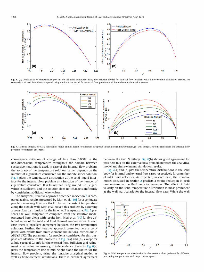
Fig. 6. (a) Comparison of temperature plot inside the solid computed using the iterative model for internal flow problem with finite element simulation results, (b)comparison of wall heat flow computed using the iterative model for external flow problem with finite element simulation results.

Fig. 7. (a) Solid temperature as a function of radius at mid-height for different air speeds in the internal flow problem, (b) wall temperature distribution in the external flowproblem for different air speeds.

Fig. 8. Wall temperature distribution in the external flow problem for differentprecooling temperatures at 0.1 m/s coolant speed.

1238 K. Shah, A. Jain / International Journal of Heat and Mass Transfer 90 (2015) 1232–1240

convergence criterion of change of less than 0.0002 in thenon-dimensional temperature throughout the domain betweensuccessive iterations is used. In case of the internal flow problem,the accuracy of the temperature solution further depends on thenumber of eigenvalues considered for the infinite series solution.Fig. 4 plots the temperature distribution at the solid–liquid inter-face for the internal flow problem as a function of the number ofeigenvalues considered. It is found that using around 8–10 eigen-values is sufficient, and the solution does not change significantlyby considering additional eigenvalues.

The analytical, iterative approach described in Section 2 is com-pared against results presented by Mori et al. [10] for a conjugateproblem involving flow in a thick tube with constant temperaturealong the outside wall. Mori et al. solved this problem by assuminga power law distribution for the inner wall temperature. Fig. 5 pre-sents the wall temperature computed from the iterative modelpresented here, along with results from Mori et al. [10] for five dif-ferent ratios of the solid and fluid thermal conductivities. In eachcase, there is excellent agreement between the two temperaturesolutions. Further, the iterative approach presented here is com-pared with results from finite-element simulations, carried out inANSYS-CFX. The parameters for problems considered for this pur-pose are identical to the problems in Fig. 3(a) and (b), except fora fluid speed of 0.1 m/s for the external flow. Sufficient grid refine-ment is carried out to ensure grid independence of results. Fig. 6(a)plots the temperature rise at mid height along the radius for theinternal flow problem, using the iterative analytical model, aswell as finite-element simulations. There is excellent agreement

between the two. Similarly, Fig. 6(b) shows good agreement forwall heat flux for the external flow problem between the analyticalmodel and finite-element simulation results.

Fig. 7(a) and (b) plot the temperature distributions in the solidbody for internal and external flow cases respectively for a numberof inlet fluid velocities. As expected, in each case, the iterativemodel discussed in Section 2 predicts a strong reduction in peaktemperature as the fluid velocity increases. The effect of fluidvelocity on the solid temperature distribution is most prominentat the wall, particularly for the internal flow case. While the wall

Fig. 9. (a) Wall heat flux distribution in the external flow problem for different air speeds for no precooling, (b) wall heat flux distribution in the external flow problem fordifferent precooling temperatures at 0.1 m/s coolant speed.

Fig. 10. Variation of the heated length in external flow as a function of air speed, (b) variation of total reversed heat in external flow problem as a function of air speed.

K. Shah, A. Jain / International Journal of Heat and Mass Transfer 90 (2015) 1232–1240 1239

temperature continues to reduce as the fluid velocity is increased,this effect saturates in regions closer to the outer wall, where theeffect of the coolant flow is not so prominent.

Fig. 8 presents results for the effect of precooling the inlet fluidin the external flow problem for a fluid velocity of 0.1 m/s. It isfound that reducing the inlet flow temperature reduces the walltemperature distribution, plotted in Fig. 8 as a function of lengthalong the cylinder. However, the effect is not very significant. Forexample, even for a precooling of �15 K, the model computationspredict a peak temperature drop of only 5 K at most.

Fig. 9(a) examines the wall heat flux from the heat-generatingsolid into the cooling fluid as a function of the coordinate alongthe flow, plotted for a number of fluid flow speeds. In each case,the wall heat flux is positive for nearly the entire length, exceptfor a small region towards the end. In this region, the sign of theheat flux reverses, and heat flows back from the fluid into the solid.This interesting phenomenon occurs because as the fluid traversesthe length of the solid, it progressively gets hotter, so that beyond acertain critical length, the heat flow direction reverses, and thefluid actually starts heating up the solid. This interesting behavioris seen at all fluid speeds. In Fig. 9(b), the wall heat flux is plottedalong the length of the plate at fluid velocity of 0.1 m/s at differentprecool temperatures. It is evident that precooling reduces thelength over which reversal of heat flow occurs. Precooling maynot affect the peak temperature of the plate significantly butmay reduce or eliminate the local heating of the plate near theend region. Such reversal in the direction of heat flow has been

reported in the past for heat transfer from a sphere in the wakeregion [39].

As shown in Fig. 10(a), the location of heat flux reversal movesfurther downstream as the fluid velocity increases. On the otherhand, the magnitude of the reversed heat flux also increases withincrease in fluid velocity. Therefore, Fig. 10(a) alone is not suffi-cient in knowing whether the overall reversed heat decreases withincrease in fluid velocity. In Fig. 10(b), total reversed heat flow isplotted against fluid velocity by integrating the reversed heat fluxover the heated length. The total reversed heat increases withincrease in velocity up to a certain velocity, after which it startsgoing down. These plots may be useful in deciding the appropriatefluid velocity, and whether precooling may be helpful in the case ofcooling a heat-generating solid with external flow.

4. Conclusions

The iterative analytical methodology presented in this paper isa general method for solving conjugate heat transfer problemsinvolving both conduction and convection. This approach is sim-pler and mathematically less involved compared to otherapproaches reported earlier. Results based on this approach arein good agreement with a past method and with finite-elementsimulations. While this method is illustrated in this paper fortwo specific example problems involving internal and externalflows, other more complicated scenarios, for example, involvingmultiple solid–fluid interfaces, can also be analyzed. The iterative

1240 K. Shah, A. Jain / International Journal of Heat and Mass Transfer 90 (2015) 1232–1240

approach presented here may help improve the fundamentalunderstanding of conjugate heat transfer, as well as develop ther-mal modeling tools for applications where conjugate heat transferis important.

Conflict of interest

None declared.

References

[1] W.M. Kays, M.E. Crawford, Convective Heat and Mass Transfer, McGraw-Hill,New York, 1993.

[2] R.K. Shah, A.L. London, Laminar flow forced convection in ducts, in: Advancesin Heat Transfer, Academic Press, New York, 1978.

[3] L. Graetz, Über die warmeleitungsfahigheit von flussingkeiten, part 1, Ann.Phys. Chem. (1883).

[4] M. Jacob, Heat Transfer, first ed., John Wiley & Sons, New York, 1949.[5] E.R.G. Eckert, R.M. Drake, Heat and Mass Transfer, McGraw-Hill, 1959.[6] E.M. Sparrow, H.S. Yu, Local non-similarity thermal boundary-layer solutions,

J. Heat Transfer 93 (1971) 328–334.[7] J.R. Sellars, M. Tribus, J.S. Klein, Heat transfer to laminar flow in a round tube or

flat conduit — the Graetz problem extended, Trans. ASME 78 (1956) 441–448.[8] M. Tribus, J.S. Klein, Forced convection from nonisothermal surfaces, in: Proc.

Heat Transfer Symp., University of Michigan Engineering Research Institute,1953, pp. 211–235.

[9] X. Yin, H.H. Bau, The conjugate Graetz problem with axial conduction, J. HeatTransfer 118 (1996) 482–485.

[10] S. Mori, M. Sakakibara, A. Tanimoto, Steady heat transfer to laminar flow in acircular tube with conduction in the tube wall, Heat Transfer Jpn. Res. 3 (1974)37–46.

[11] A.V. Luikov, V.A. Aleksashenko, A.A. Aleksashenko, Analytical methods ofsolution of conjugated problems in convective heat transfer, Int. J. Heat MassTransfer 14 (1971) 1047–1056.

[12] J. Gosse, Analyse simplifiée du couplage conduction-convection pour unécoulement à couche limite laminaire sur une plaque plane, Rev. Gen. Therm.228 (1980) 967–971.

[13] T.L. Perelman, On conjugated problems of heat transfer, Int. J. Heat MassTransfer 3 (1961) 293–303.

[14] M. Faghri, E.M. Sparrow, Simultaneous wall and fluid axial conduction inlaminar pipe-flow heat transfer, J. Heat Transfer 102 (1980) 58–63.

[15] R.K. Shah, M.S. Bhatti, Laminar convective heat transfer in ducts, in: S. Kakac,R.K. Shah, W. Aung (Eds.), Handbook of Single-phase Convective Heat Transfer,John Wiley, New York, 1987.

[16] K. Shah, A. Jain, Modeling of steady-state and transient thermal performance ofa Li-ion cell with an axial fluidic channel for cooling, Int. J. Energy Res. 39(2015) 573–584.

[17] M.N. Ozisik, Heat Conduction, second ed., John Wiley & Sons, 1993.[18] H.S. Carslaw, J.C. Jaegar, Conduction of Heat in Solids, second ed., Clarendon

Press, 1959.[19] A.S. Dorfman, Conjugate Problems in Convective Heat Transfer, CRC Press,

2009.

[20] B. Weigand, G. Gassner, The effect of wall conduction for the extended Graetzproblem for laminar and turbulent channel flows, Int. J. Heat Mass Transfer 50(2007) 1097–1105.

[21] V.A. Aleksashenkto, The steady conjugated problem of heat transfer in fluidflow in a semi-infinite tube including the effect of viscous dissipation, J. Eng.Phys. 14 (1968) 100–108.

[22] S. Mori, T. Shinke, M. Sakakibara, A. Tanimoto, Steady heat transfer to laminarflow between parallel plates with conduction in the wall, Heat Transfer Jpn.Res. 3 (1974) 37–46.

[23] C.A. Deavours, An exact solution for the temperature distribution in parallelplate Poiseuille flow, J. Heat Transfer 96 (1974) 489–495.

[24] R.O.C. Guedes, M.N. Ozisik, Conjugated turbulent heat transfer with axialconduction in wall and convection boundary conditions in a parallel-platechannel, Int. J. Heat Mass Transfer 13 (1992) 322–328.

[25] A. Lehtinen, R. Karvinen, Analytical solution for a class of flat plateconjugate convective heat transfer problems, Front. Heat Mass Transfer 2(2011) 043004.

[26] G.S. Barozzi, G. Pagliarini, A method to solve conjugate heat transfer problems:the case of fully developed laminar flow in a pipe, J. Heat Transfer 107 (1985)77–83.

[27] A. Pozzi, M. Lupo, Coupling of conduction with forced convection over a flatplate, Int. J. Heat Mass Transfer 32 (1989) 1207–1214.

[28] S. Bilir, Laminar flow heat transfer in pipes including two-dimensional walland fluid axial conduction, Int. J. Heat Mass Transfer 38 (1995) 1619–1625.

[29] P.I. Jagad, B.P. Puranik, A.W. Date, An iterative procedure for the evaluation of aconjugate condition in heat transfer problems, Numer. Heat Transfer Part AAppl. 61 (2012) 353–380.

[30] R. Karvinen, Some new results for conjugate heat transfer in a flat plate, Int. J.Heat Mass Transfer 21 (1978) 1261–1264.

[31] A. Campo, C. Schuler, Heat transfer in laminar flow through circular tubesaccounting for two-dimensional wall conduction, Int. J. Heat Mass Transfer 31(1988) 2251–2259.

[32] I. Pop, D.B. Ingham, A note on conjugate forced convection boundary-layerflow past a flat plate, Int. J. Heat Mass Transfer 36 (1993) 3873–3876.

[33] M. Vynnycky, S. Kimura, K. Kanev, I. Pop, Forced convection heat transfer froma flat plate: the conjugate problem, Int. J. Heat Mass Transfer 41 (1998)45–59.

[34] L. Choobineh, A. Jain, Determination of temperature distribution in three-dimensional integrated circuits (3D ICs) with unequally-sized die, Appl.Therm. Eng. 56 (2013) 176–184.

[35] L. Choobineh, A. Jain, Analytical solution for steady-state and transienttemperature field in vertically integrated three-dimensional integratedcircuits (3D ICs), IEEE Trans. Compon. Packag. Manuf. Technol. 2 (2012)2031–2039.

[36] A. Haji-Sheikh, J.V. Beck, D. Agonafer, Steady-state heat conduction inmultilayer bodies, Int. J. Heat Mass Transfer 46 (2003) 2363–2379.

[37] S.J. Drake, M. Martin, D.A. Wetz, J.K. Ostanek, S.P. Miller, J.M. Heinzel, A. Jain,Heat generation rate measurement in a Li-ion cell at large C-rates throughtemperature and heat flux measurements, J. Power Sources 285 (2015) 266–273.

[38] S.J. Drake, D.A. Wetz, J.K. Ostanek, S.P. Miller, J.M. Heinzel, A. Jain,Measurement of anisotropic thermophysical properties of cylindrical Li-ioncells, J. Power Sources 252 (2014) 298–304.

[39] B. Abramzon, C. Elata, Unsteady heat transfer from a single sphere in stokesflow, Int. J. Heat Mass Transfer 27 (1984) 687–695.