Interest and Equivalence

L. K. Gaafar

Interest and Equivalence

Example: You borrowed $5,000 from a bank and you have to pay it back in 5 years. There are many ways the debt can be repaid. (i = 0.08)

Plan 1: At end of each year pay $1,000 principal plus interest due.Plan 2: Pay interest due at end of each year and principal at end of five years.Plan 3: Pay in five end-of-year payments ($1,252).Plan 4: Pay principal and interest in one payment at end of five years.

All these plans are equivalent in the sense that the sum of all outgoing cash flows at time 0 is $5,000.

Present Value• Plan 1: At end of each year pay $1,000 principal plus interest due

(a) (b) (c) (d) (e) (f)Yr. Amnt. Owed Int. Owed Total Owed Princip. Total Payment Begin. of Yr 0.08 * b b + c Payment

1 $5,000 $400 $5,400 $1,000 $1,400

2 $4,000 $320 $4,320 $1,000 $1,320

3 $3,000 $240 $3,240 $1,000 $1,240

4 $2,000 $160 $2,160 $1,000 $1,160

5 $1,000 $80 $1,080 $1,000 $1,080

$1,200 $5,000 $6,200

Present Value

• Plan 2: Pay interest due at end of each year and principal at end of five years.

(a) (b) (c) (d) (e) (f)

Yr. Amnt. Owed Int. Owed Total Owed Princip. Total Payment Begin. of Yr 0.08 * b b + c Payment

1 $5,000 $400 $5,400 $0 $400

2 $5,000 $400 $5,400 $0 $400

3 $5,000 $400 $ 5,400 $0 $400

4 $5,000 $400 $ 5,400 $0 $400

5 $5,000 $400 $ 5,400 $5,000 $5,400

$2,000 $5,000 $7,000

Present Value

• Plan 3: Pay in five end-of-year payments

(a) (b) (c) (d) (e) (f)Yr. Amnt. Owed Int. Owed Total Owed Princip. Total Payment

Begin. of Yr 0.08 * b b + c Payment

1 $5,000 $400 $5,400 $852 $1,252

2 $4,148 $332 $4,480 $921 $1,252

3 $3,227 $258 $3,485 $994 $1,252

4 $2,233 $179 $2,412 $1,074 $1,252

5 $1,159 $93 $1,252 $1,159 $1,252 $1,261 $5,000 $6,261

Present Value

• Plan 4: Pay principal and interest in one payment at end of five years.

(a) (b) (c) (d) (e) (f)

Yr. Amnt. Owed Int. Owed Total Owed Princip. Total Payment Begin. of Yr 0.08 * b b + c Payment

1 $5,000 $400 $5,400 $0 $0

2 $5,400 $432 $5,832 $0 $0

3 $5,832 $467 $6,299 $0 $0

4 $6,299 $504 $6,802 $0 $0

5 $6,802 $544 $7,347 $5,000 $7,347 $2,347 $5,000 $7,347

Compound Interest: interest is charged on the unpaid interest.

Present Value

Plan 1: At end of each year pay $1,000 principal plus interest due (col. f) (col. b)

Year EOY Pay. Owed 1 $1,400 $5,000 2 $1,320 $4,000 3 $1,240 $3,000 4 $1,160 $2,000 5 $1,080 $1,000

$6,200 $15,000

$ Owed

$0

$1,000

$2,000

$3,000

$4,000

$5,000

$6,000

1 2 3 4 5

Time (Years)

$ Owed

Present Value

Plan 2: Pay interest due at end of each year and principal at end of five years.

Year EOY Pay. Owed 1 $400 $5,000 2 $400 $5,000 3 $400 $5,000 4 $400 $5,000 5 $5,400 $5,000

$7,000 $25,000

$ Owed

$0

$1,000

$2,000

$3,000

$4,000

$5,000

$6,000

1 2 3 4 5

Time (Years)

$ Owed

Present Value

Plan 3: Pay in five end-of-year payments

Year EOY Pay. Owed 1 $1,252 $5,000 2 $1,252 $4,148 3 $1,252 $3,227 4 $1,252 $2,233 5 $1,252 $1,159

$6,261 $15,767

$ Owed

$0

$1,000

$2,000

$3,000

$4,000

$5,000

$6,000

1 2 3 4 5

Time (Years)

$ Owed

Present Value

Plan 4: Pay principal and interest in one payment at end of five years.

Year EOY Pay. Owed 1 $0 $5,000 2 $0 $5,400 3 $0 $5,832 4 $0 $6,299 5 $7,347 $6,802

$7,347 $29,333

$ Owed

$0$1,000$2,000$3,000$4,000$5,000$6,000$7,000$8,000

1 2 3 4 5

Time (Years)

$ Owed

Present Value

Summary of Payment Plans (a) (b) (c) (d)

Plan Total Paid Tot. Int. Area under Ratio: curve (b)/(c)

1 $6,200 $1,200 $15,000 0.08 2 $7,000 $2,000 $25,000 0.08 3 $6,261 $1,261 $15,767 0.08 4 $7,347 $2,347 $29,333 0.08

Key Question. What common property do all four plans have? Conclusion: interest rate = (total int. paid)/(area under curve) or total int. paid = (interest rate) * (area under curve) Since the areas under the curve vary for the 4 plans, but the interest rate does not, the total interest paid also varies.

Interest and Equivalence

Example: You borrowed $8,000 from a bank and you have to pay it back in 4 years. There are many ways the debt can be repaid. (i = 0.10)

Plan 1: At end of each year pay $2,000 principal plus interest due.Plan 2: Pay interest due at end of each year and principal at end of four years.Plan 3: Pay in four end-of-year payments ($2,524).Plan 4: Pay principal and interest in one payment at end of four years.

ExampleWith i = 10%, n = 4, find an equivalent uniform payment A for:

2400018000

120006000

1 2 3 40

Possible SolutionThis is a problem with decreasing costs instead of increasing costs. Note we can write it as the DIFFERENCE of the following two diagrams, the second of which is in the standard form we need, the first of which is a series of uniform payments.

-

A = 24000

0 600

1200

1800

We conclude now that:A = 24000 – 6000 (A/G,10%,4) = 24000 –6000(1.381) = 15,714.

Possible Solution24000

1800012000

6000

1 2 3 40

24000

1 2 3 40

24000 24000 24000

600012000

18000

Nominal/Effective Rates

Suppose that a $1,000 lump-sum amount is invested for 10 years at a nominal interest rate of 6% compounded quarterly. How much is it worth at the end of the tenth year?

Nominal/Effective Rates

Suppose that one has a bank loan for $10,000, which is to be repaid at equal end-of-month installments for five years with a nominal interest rate of 12% compounded monthly. What is the amount of each payment?

Nominal/Effective Rates

What is the present worth of 8 end-of-quarter payment of $1,000 each, if the nominal interest rate is 15% compounded monthly?

Nominal/Effective RatesSuppose that there exists a series of 10 end-of-year receipts of $1,000 each. What is their equivalent worth as of the end of the tenth year if the nominal interest rate is 12% compounded quarterly? ($18,021)

Comparing AlternativesThe table below shows the cash flows associated with 6 mutually exclusive investment opportunities. If the MARR is 10%, identify the feasible alternatives and choose the best one. All alternatives have a useful life of 10 years.

Alternative

A B C D E F

Capital Investment (P) -$900 -$1,500 -$2,500 -$4,000 -$5,000 -$7,000

Annual Revenue (A) $150 $276 $400 $925 $1,125 $1,425

The key to solving this problem is to realize that each alternative provides us with an opportunity to invest P for an annual return of A. Acceptable alternatives are those that allow us to realize 10% or more on our investment (P). In other words, we are trying to judge whether it is better to invest P at the rate of i (10%), or invest it for the return of A every period (accept the alternative).

Present Worth (PW) ComparisonsPresent worth evaluations assess the value of all cash flows at time 0. In the given problem, we are trying to evaluate whether an annual return (A) realizes a specific return (profit, i) on an initial investment (P).

The PW of the given cash flows is:

PW = -P + A (P/A, i, 10).

A

1 20 3 9 10

P

i = MARR = 10%

A positive PW [A (P/A, i, 10) > P] indicates that the investment opportunity provides an annual return that is higher than investing the amount P at the MARR (i). In other words, the given return (A) realizes a higher profit than the targeted (i), and accordingly a favorable investment opportunity for P. Another way to look at a positive PW is that the targeted return rate (i) may be realized with a smaller investment (P-PW).

A PW of 0 indicates that the investment opportunity realizes exactly the targeted return rate (i), and hence, a borderline investment opportunity.

A negative PW [A (P/A, i, 10) < P] indicates that the rate of return is less than the targeted (i), and accordingly an unacceptable investment opportunity. In other words, it is better to invest the amount P at the rate i than to invest it for an annual return of A.

For both cases when PW 0, the IRR method may be used to calculate the exact rate of return.

PW = ?

The best alternative is the one with the highest positive PW

Future Worth (FW) ComparisonsFuture worth evaluations assess the value of all cash flows at time n. In the given problem, we are trying to evaluate whether an annual return (A) realizes a specific return (profit, i) on an initial investment (P).

The FW of the given cash flows is:

FW = -P(F/P, i, 10) + A (F/A, i, 10).

A

1 20 3 9 10

P

i = MARR = 10%

A positive FW [A (F/A, i, 10) > P (F/P, i, 10)] indicates that the future value of the annuity (A) is higher that that of the initial investment (P), and hence, a favorable investment opportunity. In other words, getting A every period is better than investing P at the MARR (i). It also means that the given return (A) realizes a higher profit than the targeted (i).

A FW of 0 indicates that the investment opportunity realizes exactly the targeted return rate (i), and hence, a borderline investment opportunity.

A negative FW [A (F/A, i, 10) < P (F/P, i, 10)] indicates that the rate of return is less than the targeted (i), and accordingly an unacceptable investment opportunity. In other words, it is better to invest the amount P at the rate i than to invest it for an annual return of A.

For both cases when FW 0, the IRR method may be used to calculate the exact rate of return.

FW = ?

The best alternative is the one with the highest positive FW

Annual Worth (AW) ComparisonsAnnual worth evaluations assess the annual resultant of all cash flows. In the given problem, we are checking that the offered annuity is at least equal to the annuity we could get by investing P at the MARR (i). Accordingly, the AW of the given cash flows is defined as:

AW = -P(A/P, i, 10) + A.

A

1 20 3 9 10

Pi = MARR = 10%

A positive AW [A > P (A/P, i, 10)] indicates that the offered annuity is greater than what we could get by investing P at the MARR (i), and hence, a favorable investment opportunity. In other words, getting A every period is better than investing P at the MARR (i). It also means that the given return (A) realizes a higher profit than the targeted (i).

An AW of 0 indicates that the investment opportunity realizes exactly the targeted return rate (i), and hence, a borderline investment opportunity.

A negative AW [A < P (A/P, i, 10)] indicates that the rate of return is less than the targeted (i), and accordingly an unacceptable investment opportunity. In other words, it is better to invest the amount P at the rate i than to invest it for an annual return of A.

For both cases when AW 0, the IRR method may be used to calculate the exact rate of return.

AW = ?

The best alternative is the one with the highest positive AW

-P(A/P, i, 10)

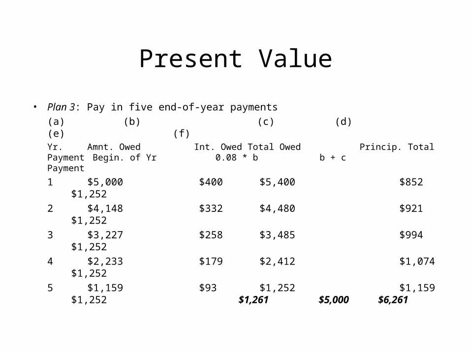
Internal Rate of Return (IRR) Comparisons

IRR evaluations assess the rate of return at which the net cash flow is equal to zero. It is the rate at which the net worth (Present, Future, or Annual) of all cash flows equals 0. A favorable opportunity exists when IRR MARR.

In our case, IRR is the actual interest at which a one time deposit P results in an annual return of A.

Notice that:

•PW, FW, AW > 0 correspond to IRR > MARR,

•PW, FW, AW < 0 correspond to IRR < MARR,

•PW, FW, AW = 0 correspond to IRR = MARR.

In other words, a negative PW, FW, or AW does not necessarily mean a loss, but merely a return rate that is smaller than the MARR.

•Acceptable alternatives are those for which IRR MRR.•Ranking Alternatives can only be based on relative comparisons.

1 20 3 9 10

P

i (IRR) = ?

A

Comparison Results

The table below shows the results of the various calculations. Alternative C may be rejected based on its negative net worth. Notice, however, that this doesn’t mean it is unprofitable. It only means that its profit (internal rate of return) is less than the MARR.

1 20 3 9 10

P

A

Alternative A B C D E FPW 21.69 195.90 -42.17 1683.72 1912.64 1756.01FW 56.25 508.12 -109.39 4367.15 4960.89 4554.63AW 3.53 31.88 -6.86 274.02 311.27 285.78IRR 10.558% 12.961% 9.606% 19.097% 18.314% 15.566%

Among all remaining alternatives, E is the best followed by F, D, B, A, respectively. PW, FW, AW results all point to the same ranking. IRR results, however, lead to a different ranking. In the table above, while D has a higher IRR, it is applied to a smaller investment (4,000), while the slightly lower rate of E gives a higher overall return when applied to the higher investment (5,000), and hence, E is better than D. Accordingly, IRR can only be used in relative comparisons (see next slide).

Relative Comparison Results (IRR)

In relative comparisons, alternatives are ranked in an ascending order of their initial investments. The IRR of the difference cash flows between the first two alternatives is evaluated. If the resulting IRR is greater than the MARR, the second alternative is better and is used as a base for further comparisons.

1 20 3 9 10

P

A

The relative IRR results in the table below agree with those of the net worth methods.

Alternative B-A D-B E-D F-E F-DIRR 16.401% 22.567% 15.098% 8.144% 10.558%

Payback (Payout) Period Method

Simple Payback ():1 20 ’-1 ’

P

Example:

A piece of new equipment has been proposed by engineers to increase the productivity of a certain manual welding operation. The investment cost is $25,000, and the equipment will have a salvage value of $5,00 at the end of its life. Increased productivity attributed to equipment will amount to $8,000 per year after taxes. Find the payback period for this investment assuming MARR = 20%.

Discounted Payback (’):

R2R1 R’R-1

E2E1 EE-1

S

0)',,/(),,/)(('

1

PiFPSkiFPERk

kk

involvedareannuitiesuniformonlywhenA

PtoreducesPER

kkk

,0)(1

Time value of money not considered.Salvage value not considered.Used as a rough estimate and a starting point for discounted.

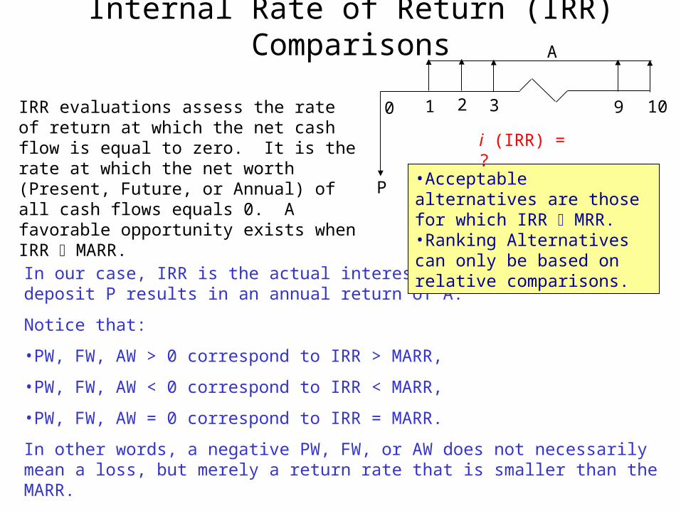
Payback Period- Example

Simple Payback ():

1 20 ’-1 ’

PDiscounted Payback (’):

S

A piece of new equipment has been proposed by engineers to increase the productivity of a certain manual welding operation. The investment cost is $25,000, and the equipment will have a salvage value of $5,00 at the end of its life. Increased productivity attributed to equipment will amount to $8,000 per year after taxes. Find the payback period for this investment assuming MARR = 20%.

4125.3000,8

000,25

A

P

86.1878)4,,/(),,/)((4

1

PiFPSkiFPERk

kk

28.934)5,,/(),,/)((5

1

PiFPSkiFPERk

kk

Try 4

Try 5

A

Bonds

Bonds are money guarantees that pay a fixed amount per period and a final amount at the end of their life (maturity). This final amount is called the redemption value. Bonds are bought for a value called the face value and usually pay a fixed amount every period that is a percentage of the face value. A bond is said to be redeemed at par value when the redemption value is the same as the face value.

Bonds pause an interesting problem when they are traded before their maturity as an investment to earn a interest other than the one they provide.

Bonds

Find the current price of a 10-year bond paying 6% per year (payable semi-annually) that is redeemed at par value, if bought by a purchaser to yield 10% per year. The face value of the bond is $1,000. [761.16]

Bonds

A certain 8-year bond has a face value of $10,000. The bond pays a nominal interest rate of 8% every three months. A prospective buyer would like to earn a nominal interest of 10% per year. How much should this buyer pay for the bond? [$8,907.55]

Bonds

A bond with a face vale of $5,000 pays interest of 8% per year. This bond will be redeemed at par value at the end of its 20-year life, an the first interest payment is due one year from now.

a. How much should be paid now for this bond in order to yield 10% per year? [$4,148.44]

b. If the bond is purchased for $4,600, what annual yield would the buyer receive? [8.9%]

Benefit/Cost RatioFor Evaluating Public Projects

Conventional B/C Ratio )&()(

)(

)cos(

)(/

MOPWSPWI

BPW

tstotalPW

benefitsPWCB

)&(

)(

)cos(

)(/

MOAWCR

BAW

tstotalAW

benefitsAWCB

Modified B/C Ratio

CR

MOAWBAWCB

)&()(/

)(

)&()(/

SPWI

MOPWBPWCB

Benefit/Cost RatioFor Evaluating Public Projects

A city is considering extending the runways of its Municipal Airport so that commercial jets can use the facility. The land can be purchased for $350,000. Construction costs are projected to be $600,000, and the additional annual maintenance costs for the runway are $22,500. The additional annual maintenance costs of the new terminal are $75,000. The increase in flights will require two new air traffic controllers at the cost of $100,000 per year. Annual benefits of the runway extension are estimated as follows:$325,000 from rental receipts.$65,000 airport tax charged to passengers.$50,000 convenience benefits.$50,000 from tourism.

Use B/C ratio to justify the project, assuming a study period of 20 years and an interest rate of 10%. [1.59, 2.62]