
INTERACTION BETWEEN DRILLED SHAFT AND MECHANICALLY ...
234
INTERACTION BETWEEN DRILLED SHAFT AND MECHANICALLY STABILIZED EARTH (MSE) WALL A Dissertation by MOHAMMAD AGHAHADI FOROOSHANI Submitted to the Office of Graduate and Professional Studies of Texas A&M University in partial fulfillment of the requirements for the degree of DOCTOR OF PHILOSOPHY Chair of Committee, Marcelo Sanchez Co-Chair of Committee, Jean-Louis Briaud Committee Members, Charles Aubeny Robert Warden Head of Department, Robin Autenrieth December 2014 Major Subject: Civil Engineering Copyright 2014 Mohammad Aghahadi Forooshani
Transcript of INTERACTION BETWEEN DRILLED SHAFT AND MECHANICALLY ...
INTERACTION BETWEEN DRILLED SHAFT AND
MECHANICALLY STABILIZED EARTH (MSE) WALL
A Dissertation
by
MOHAMMAD AGHAHADI FOROOSHANI
Submitted to the Office of Graduate and Professional Studies of Texas A&M University
in partial fulfillment of the requirements for the degree of
DOCTOR OF PHILOSOPHY
Chair of Committee, Marcelo Sanchez Co-Chair of Committee, Jean-Louis Briaud
Committee Members, Charles Aubeny Robert Warden Head of Department, Robin Autenrieth
December 2014
Major Subject: Civil Engineering
Copyright 2014 Mohammad Aghahadi Forooshani

ii
ABSTRACT
Drilled shafts under horizontal loads are being constructed within Mechanically
Stabled Earth (MSE) walls in the reinforced zone especially in overpass bridges and traffic
signs. The interaction between the drilled shafts and the MSE wall is not well known and
not typically incorporated in the design. To better understand the interaction, a full scaled
test was conducted in 2012 at Texas A&M University. The test was performed on an MSE
wall with backfill material of clean sand and soil reinforcements of metal strips. Also a
real project was instrumented during construction and data gathered for couple of months
from this project. Numerical model was used for further investigation and it was calibrated
by the test results and the data from monitoring the real site.
Main focus in this research was on the MSE walls with metal strips and a
detailed study was performed on the friction mechanism of metal strips. Numerical
modeling was used to better understand the friction factor and the relation between the
depth of reinforcement and the maximum tension in the strip. Also some numerical
simulations were performed to better understand the effect of number of bumps per foot
on the metal strips on the friction factor. The other part of the numerical study was focused
on the effect of the shape of the bumps on the strips. Accordingly different strips were
modeled with different numbers of bumps and with different bump shapes.
Sensitivity analysis and parametric study were performed and 64 numerical
cases were modeled to understand the effect of different parameters on the interaction
between the MSE wall and the drilled shaft.

iii
The data from different numerical simulations, the full-scale test and the
monitoring of the real site were processed and a modification to the current guideline was
proposed for the case where there is a horizontally drilled shaft in the reinforced zone of
the MSE wall. One of the final results of this research is a design chart which can help the
designer of MSE walls with laterally loaded drilled shaft in the reinforced zone of the wall,
to take the additional pressure on the wall according to the drilled shaft into the final
design.

iv
DEDICATION
This dissertation is dedicated to my brilliant and outrageously loving and
supporting wife, Ladan whose affection, love, encouragement and prays made me to get
such success and honor. A special gratitude to my loving parents whose words of
encouragement and support ring in my ear and first taught me the value of education.

v
ACKNOWLEDGEMENTS
I would like to thank my committee chairs, Dr.Sanchez and Dr.Briaud, and my
committee members, Dr. Aubeny, Dr. Warden for their guidance and support throughout
the course of this research.
Thanks also go to my friends and colleagues and the department faculty and staff
for making my time at Texas A&M University a great experience. I also want to extend
my gratitude to Texas Department of Transportation (TxDOT) and Texas transportation
Institute (TTI), which supported this research.

vi
TABLE OF CONTENTS
Page
ABSTRACT ...................................................................................................................... ii
DEDICATION ..................................................................................................................iv
ACKNOWLEDGEMENTS ...............................................................................................v
TABLE OF CONTENTS ..................................................................................................vi
LIST OF FIGURES ...........................................................................................................ix
LIST OF TABLES ..........................................................................................................xix
1.INTRODUCTION ........................................................................................................... 1
1.1.Background ......................................................................................................... 1 1.2.Motivation ........................................................................................................... 1 1.3.Objectives ........................................................................................................... 2 1.4.Activities ............................................................................................................. 3 1.5.Accomplishments ............................................................................................... 4
1.6.Dissertation organization .................................................................................... 6
2.LITERATURE REVIEW ................................................................................................ 8
2.1.Introduction ......................................................................................................... 8 2.2.Current practice ................................................................................................ 10 2.3.Current research status ...................................................................................... 17 2.4.Research outcomes of KDOT and UDOT research .......................................... 19
2.4.1.KODT research .................................................................................... 19
2.4.2.UDOT research .................................................................................... 23 2.4.3.Instrumentation of KDOT and UDOT research ................................... 26
2.5.Other background information ......................................................................... 27
2.6.Conclusion ........................................................................................................ 27
3.INSTRUMENTATION DESIGN ................................................................................. 29
3.1.Instrumentation used in previous works ........................................................... 29 3.2.Adopted instrumentation .................................................................................. 34
3.2.1.Shaft and wall deflection ...................................................................... 35 3.2.2.Earth pressure ....................................................................................... 35

vii
3.2.3.Load in reinforcements ........................................................................ 36 3.2.4.Data acquisition system ....................................................................... 36 3.2.5.Power supply ........................................................................................ 39
3.3.Adopted instrumentation .................................................................................. 39 3.3.1.Tiltmeter ............................................................................................... 41 3.3.2.Inclinometer ......................................................................................... 42 3.3.3.Photogrammetry ................................................................................... 44 3.3.4.Pressure cells ........................................................................................ 45 3.3.5.Strain gauges ........................................................................................ 46 3.3.6.Data acquisition system ....................................................................... 51
3.4.Conclusion ........................................................................................................ 54
4.FIELD STUDIES-TESTS AND MONITORING ......................................................... 55
4.1.Introduction ....................................................................................................... 55 4.2.Full-scale loading test ....................................................................................... 56
4.2.1.Overview .............................................................................................. 56 4.2.2.Wall detail ............................................................................................ 57 4.2.3.Backfill material ................................................................................... 59 4.2.4.Wall reinforcement............................................................................... 64 4.2.5.Drilled shaft .......................................................................................... 65 4.2.6.Instrumentation .................................................................................... 66 4.2.7.Construction of the wall ....................................................................... 82
4.2.8.Loading test .......................................................................................... 89 4.2.9.Main results associated with the loading test ....................................... 92 4.2.10.Discussion ........................................................................................ 129
4.3.Monitoring at TxDOT site at Bastrop ............................................................. 129 4.3.1.Real project introduction .................................................................... 129
4.4.Conclusion ...................................................................................................... 144
5.NUMERICAL MODELING ....................................................................................... 145
5.1.Introduction ..................................................................................................... 145
5.2.Simulation of the pullout test with cable elements ......................................... 145 5.3.Modeling the pull-out tests discretizing the strip in the mesh ........................ 149
5.4.Simulation of the Load Test at Riverside Campus ......................................... 153 5.4.1.Natural soil ......................................................................................... 155 5.4.2.Backfill soil ........................................................................................ 156 5.4.3.Drilled shaft ........................................................................................ 159 5.4.4.Wall panels ......................................................................................... 159
5.4.5.MSE wall model ................................................................................. 160 5.4.6.Loading protocol ................................................................................ 161
5.5.Parametric study ............................................................................................. 173 5.5.1.Outline of the parametric study .......................................................... 173

viii
5.5.2.Baseline case ...................................................................................... 176 5.5.3.Effect of different parameters ............................................................ 176
5.6.Conclusion ...................................................................................................... 181
6.ANTICIPATED DESIGN METHOD ......................................................................... 182
6.1.Introduction ..................................................................................................... 182 6.2.Design method without the drilled shaft ......................................................... 182
6.2.1.Pull-out design ................................................................................... 182 6.2.2.Yield of the reinforcement design ...................................................... 185
6.3.MSE wall design the drilled shaft ................................................................... 185
6.3.1.Parameters to be studied..................................................................... 186 6.3.2.Numerical cases ................................................................................. 188 6.3.3.Pressure distribution on the panels ..................................................... 192 6.3.4.Proposed design guideline.................................................................. 196
6.4.Comparison between AASHTO design and proposed design ........................ 200 6.5.General considerations .................................................................................... 203 6.6.Conclusion ...................................................................................................... 204
7.CONCLUSIONS AND PROPOSAL FOR FUTURE WORKS ................................. 205
7.1.Summary and conclusions .............................................................................. 205 7.2.Proposal for future works ............................................................................... 207
REFERENCES ............................................................................................................... 209

ix
LIST OF FIGURES
Page
Figure 2-1 Retaining walls used by TxDOT from August 1, 2006 through June 20, 2007 (Modified from (Chen et al., 2007)) .......................................................... 9
Figure 2-2 Drilled shafts within MSE wall: (a) construction of drilled shaft behind MSE wall, and (b) drilled shafts behind MSE wall supporting bridge abutment (After Anderson, 2005). .................................................................... 10
Figure 2-3 Typical failure modes for MSE walls ............................................................. 14
Figure 2-4 Lateral earth pressure induced by laterally loaded drilled shaft (Berg et al. 2009) ................................................................................................................. 16
Figure 2-5 Conflict of shafts and reinforcement: (a) construction obstruction; (b) rearrangement of reinforcement (Berg et al. 2009) .......................................... 17
Figure 2-6 Studies on the interaction between MSE walls and drilled shafts .................. 18
Figure 2-7 Plan view of MSE test wall and shafts (Tensar 2007) .................................... 20
Figure 2-8 Full-scale tests: (a) single shaft; and (b) group shafts .................................... 21
Figure 2-9 Design chart for drilled shaft .......................................................................... 22
Figure 2-10 Conceptual sketch of UDOT research (Rollins et al. 2010) ......................... 24
Figure 2-11 Test setup ...................................................................................................... 24
Figure 2-12 Field tests (Rollins et al. 2010) ..................................................................... 25
Figure 2-13 Passive force-deflection curves (Rollins et al. 2010) ................................... 25
Figure 3-1 Installation of earth pressure cells (M. C. Pierson et al., 2009) ..................... 30
Figure 3-2 Installation of load cells and LVDTs (M. C. Pierson et al., 2009) ................. 31
Figure 3-3 Installation of photogrammetry targets (M. C. Pierson et al., 2009) .............. 32
Figure 3-4 Schematic representation of instrumentation (plan view) .............................. 37

x
Figure 3-5 Schematic representation of instrumentation (cross section view) ................ 38
Figure 3-6 Tiltmeter used in the project ........................................................................... 41
Figure 3-7 Inclinometer .................................................................................................... 43
Figure 3-8 Photogrammetry ............................................................................................. 45
Figure 3-9 Clean the strip surface by sand paper ............................................................. 48
Figure 3-10 Installed strain gauges .................................................................................. 49
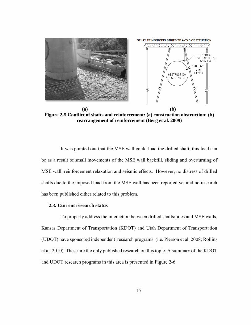
Figure 3-11 Testing strip with strain gauges .................................................................... 50
Figure 3-12 Calibration results ......................................................................................... 51
Figure 3-13 CR1000 data logger ...................................................................................... 52
Figure 3-14 SP10-10W solar panel .................................................................................. 53
Figure 3-15 PS100 rechargeable power supply ................................................................ 53
Figure 4-1 Wall detail ...................................................................................................... 57
Figure 4-2 Panel details .................................................................................................... 58
Figure 4-3 Gradation curve for backfill material ............................................................. 59
Figure 4-4 Stress-strain curve for σ3=7KPa..................................................................... 60
Figure 4-5 Volumetric strain vs. axial strain for σ3=7KPa .............................................. 61
Figure 4-6 Stress-strain curve for σ3=14KPa................................................................... 61
Figure 4-7 Volumetric strain vs. axial strain for σ3=14KPa ............................................ 61
Figure 4-8 Stress-strain curve for σ3=31KPa................................................................... 62
Figure 4-9 Volumetric strain vs. axial strain for σ3=31KPa ............................................ 62
Figure 4-10 Triaxial result for backfill material ............................................................... 63
Figure 4-11 Results in s-t plain ........................................................................................ 63

xi
Figure 4-12 Details of metal strip (The Reinforced Earth Company 2005) ..................... 64
Figure 4-13 Photos of the trips provided by RECO ......................................................... 65
Figure 4-14 Drilled shaft detail ........................................................................................ 66
Figure 4-15 Rotating machine with sand paper ............................................................... 68
Figure 4-16 Clean and shiny surface ................................................................................ 69
Figure 4-17 Strain gauge and connector installed using super glue ................................. 69
Figure 4-18 Protecting strain gauges and connectors using PVC tape ............................ 70
Figure 4-19 Tiltmeter used in this project ........................................................................ 71
Figure 4-20 Aluminum box used to protect tiltmeter ....................................................... 71
Figure 4-21 Pressure cell used in the test ......................................................................... 73
Figure 4-22 Manually compacted area between two pressure cells ................................. 73
Figure 4-23 Inclinometer probe ........................................................................................ 74
Figure 4-24 Detail of the casing ....................................................................................... 75
Figure 4-25 Photogrammetry signs .................................................................................. 76
Figure 4-26 PVC tube used for photogrammetry ............................................................. 78
Figure 4-27 Floor drain used to install PVC tubes on the wall ........................................ 78
Figure 4-28 Sample photo that used for photogrammetry ............................................... 79
Figure 4-29 String pot used in this project ....................................................................... 80
Figure 4-30 Fixed point and string pots ........................................................................... 80
Figure 4-31 Hydraulic jack............................................................................................... 81
Figure 4-32 Pump for hydraulic jack ............................................................................... 81
Figure 4-33 Load frame on (a) the pavement (b) the drilled shaft ................................... 82

xii
Figure 4-34 Details of loading frames .............................................................................. 83
Figure 4-35 Excavation .................................................................................................... 83
Figure 4-36 Wall foundation ............................................................................................ 84
Figure 4-37 First rows of panels ...................................................................................... 85
Figure 4-38 Drilled shaft behind the wall ........................................................................ 86
Figure 4-39 First layer compaction .................................................................................. 86
Figure 4-40 Installed strips (first layer) ............................................................................ 87
Figure 4-41 Nuclear density test ..................................................................................... 88
Figure 4-42 Compaction curve ......................................................................................... 88
Figure 4-43 Photo taken during the load test ................................................................... 89
Figure 4-44 Main positons asscociated with the loading test ........................................... 90
Figure 4-45 Loading steps ................................................................................................ 91
Figure 4-46 Load-displacement for drilled shaft .............................................................. 93
Figure 4-47 Load-displacement for wall .......................................................................... 93
Figure 4-48 Plot showing the drilled shaft against the wall displacement ....................... 94
Figure 4-49 Strips numbers and positions ........................................................................ 95
Figure 4-50 Strip with four strain gauges (S-4-1). ........................................................... 96
Figure 4-51 Force in the strip S-4-1 excluding Geostatic force ....................................... 97
Figure 4-52 Force in the strip S-4-1 including Geostatic force ........................................ 97
Figure 4-53 Two strain gauge strip .................................................................................. 98
Figure 4-54 Force in the strip S-2-1 excluding geostatic force ........................................ 99
Figure 4-55 Force in the strip S-2-2 excluding geostatic force ........................................ 99

xiii
Figure 4-56 Force in the strip S-2-1 including geostatic force....................................... 100
Figure 4-57 Force in the strip S-2-2 including geostatic force....................................... 100
Figure 4-58 Force in the strips ....................................................................................... 101
Figure 4-59 Force in the strips ....................................................................................... 101
Figure 4-60 Force in the strips ....................................................................................... 102
Figure 4-61 Force in the strips ....................................................................................... 102
Figure 4-62 Force in the strips ....................................................................................... 102
Figure 4-63 Force in the strips ....................................................................................... 102
Figure 4-64 Force in the strips ....................................................................................... 103
Figure 4-65 Force in the strips ....................................................................................... 103
Figure 4-66 Force in the strips ....................................................................................... 104
Figure 4-67 Force in the strips ....................................................................................... 104
Figure 4-68 Force in the strips ....................................................................................... 104
Figure 4-69 Force in the strips ....................................................................................... 104
Figure 4-70 Distribution of forces at each side of the drilled shaft in first layer of strips. The “0” corresponds to the position of the drilled shaft ...................... 106
Figure 4-71 Distribution of forces at each side of the drilled shaft in second layer of strips. The “0” corresponds to the position of the drilled shaft ...................... 106
Figure 4-72 Distribution of forces at each side of the drilled shaft in first layer of strips including Geostatic loads. The “0” corresponds to the position of the drilled shaft ..................................................................................................... 107
Figure 4-73 Distribution of forces at each side of the drilled shaft in second layer of strips including Geostatic loads. The “0” corresponds to the position of the drilled shaft ..................................................................................................... 107
Figure 4-74 Pressure measured on the drilled shaft with the load cell........................... 108

xiv
Figure 4-75 Pressure measured on the wall with the load cell ....................................... 109
Figure 4-76 Tiltmeter result for the device installed on top of the drilled shaft ............ 110
Figure 4-77 Tiltmeter result for the device installed on bottom of the drilled shaft ...... 110
Figure 4-78 Tiltmeter result for the device installed on top of the wall ......................... 111
Figure 4-79 Tiltmeter result for the device installed on bottom of the wall .................. 111
Figure 4-80 Drilled shaft deformation profile for horizontal load of 40 kips ................ 113
Figure 4-81 Plan view of the drilled shaft deformation for horizontal load of 40 kips . 114
Figure 4-82 Wall deformation profile for horizontal load of 40 kips ............................ 115
Figure 4-83 Plan view of the wall deformation for horizontal load of 40 kips .............. 116
Figure 4-84 Drilled shaft deformation profile for horizontal load of 35 kips ................ 117
Figure 4-85 Plan view of the drilled shaft deformation for horizontal load of 35 kips . 118
Figure 4-86 Wall deformation profile for horizontal load of 35 kips ............................ 119
Figure 4-87 Plan view of the wall deformation for horizontal load of 35 kips .............. 120
Figure 4-88 Comparison between tiltmeter and inclinometer for top of the drilled shaft ................................................................................................................. 121
Figure 4-89 Comparison between tiltmeter and inclinometer for bottom of the drilled shaft ................................................................................................................. 121
Figure 4-90 LIDAR plan views of the drilled shaft and the wall for initial condition ... 123
Figure 4-91 LIDAR plan views of the drilled shaft and the wall at the end of the test . 123
Figure 4-92 Wall deformation contour for horizontal load of 5 kips ............................. 125
Figure 4-93 Wall deformation contour for horizontal load of 10 kips ........................... 125
Figure 4-94 Wall deformation contour for horizontal load of 15 kips ........................... 126
Figure 4-95 Wall deformation contour for horizontal load of 20 kips ........................... 126

xv
Figure 4-96 Wall deformation contour for horizontal load of 25 kips ........................... 127
Figure 4-97 Wall deformation contour for horizontal load of 30 kips ........................... 127
Figure 4-98 Wall deformation contour for horizontal load of 35 kips ........................... 128
Figure 4-99 Wall deformation contour for horizontal load of 40 kips ........................... 128
Figure 4-100 Location for project in Bastrop ................................................................. 130
Figure 4-101 Plan view of the overpass ......................................................................... 131
Figure 4-102 East wall detail ......................................................................................... 131
Figure 4-103 Drilling the hole for the inclinometer casing ............................................ 133
Figure 4-104 Extended casing attached to the wall ........................................................ 133
Figure 4-105 Casing at top of the wall ........................................................................... 134
Figure 4-106 Tiltmeters installed on the wall ................................................................ 135
Figure 4-107 PVC tubes used for protecting wires ........................................................ 135
Figure 4-108 First and second layers of grids ................................................................ 136
Figure 4-109 Strain gauge installed on the bar .............................................................. 137
Figure 4-110 Strips attached to the bars ......................................................................... 137
Figure 4-111 Sand bags for protecting the gauges ......................................................... 138
Figure 4-112 Sand bag used on pressure cell to uniform the pressure ........................... 139
Figure 4-113 Data Acquisition installed at Bastrop site a) Box b) Solar panel ............. 140
Figure 4-114 Strain gauge numbering ............................................................................ 141
Figure 4-115 Strain gauge data from Bastrop site .......................................................... 141
Figure 4-116 Pressure cell data for Bastrop site ............................................................ 142
Figure 4-117 Tiltmeter data from Bastrop site ............................................................... 143

xvi
Figure-4-118 Inclinometer results for Bastrop site a) toward the wall b) parallel with the wall ............................................................................................................ 144
Figure 5-1 Shear spring modulus (Itasca, 2006) ............................................................ 146
Figure 5-2 Pullout test results for 2.44 m long strip at different depth (William D. Lawson, 2011) ................................................................................................ 147
Figure 5-3 Calibration of shear spring for metal strips .................................................. 148
Figure 5-4 FLAC 3D model of pullout test for 8ft strip in depth of 5 ft ........................ 148
Figure 5-5 Results for test and modeling of pullout for 8ft strip in depth of 5 ft ........... 149
Figure 5-6 Pullout resistance factor vs. depth ................................................................ 150
Figure 5-7 Detail of modeled strip (actual strip) ............................................................ 151
Figure 5-8 Completed model of actual strip ................................................................... 151
Figure 5-9 Detail of modeled strip with 60 bumps per foot ........................................... 152
Figure 5-10 Results of the modeling the actual strip and pull-out test .......................... 152
Figure 5-11 Friction factor for different cases ............................................................... 153
Figure 5-12 Natural soil PMT result at different depth .................................................. 156
Figure 5-13 Triaxial result for backfill material ............................................................. 158
Figure 5-14 Backfill PMT results at different depth ...................................................... 158
Figure 5-15 Loading steps .............................................................................................. 162
Figure 5-16 Different parts of the MSE wall Model ...................................................... 163
Figure 5-17 Deformation of the wall after applying 25 kips of horizontal load ............ 164
Figure 5-18 Deformation of the wall after applying 40 kips of horizontal load ............ 165
Figure 5-19 Deformation of the drilled shaft and the MSE wall (a) side view (b) top view ................................................................................................................. 165

xvii
Figure 5-20 Deformation of top of the shaft for the test and model .............................. 166
Figure 5-21 Deformation of top of the wall for the test and model ............................... 167
Figure 5-22 Forces in the strips after horizontal load of 25 kips ................................... 168
Figure 5-23 Force in the strip “S-4-1-B” according to (a) horizontal load on the shaft (b) wall displacement ...................................................................................... 169
Figure 5-24 Forces in the strip for different Фs .............................................................. 170
Figure 5-25 Plastic zone for different values of horizontal load on top of the drilled shaft ................................................................................................................. 171
Figure 5-26 Geometry of the case without the wall ....................................................... 172
Figure 5-27 Comparison between the case with the wall and the case without the wall ................................................................................................................. 173
Figure 5-28 Numerical model for drilled shaft within the MSE wall ............................ 174
Figure 5-29 Numerical model for drilled shaft without the MSE wall .......................... 175
Figure 5-30 Drilled shaft deflection for different D/B ................................................... 177
Figure 5-31 MSE wall deflection for different D/B ....................................................... 178
Figure 5-32 Drilled shaft deflection for different embedded depth ............................... 179
Figure 5-33 Drilled shaft deflection for different backfill material ............................... 180
Figure 5-34 MSE wall deflection for different backfill material ................................... 180
Figure 6-1 Required length of strip in the failure zone .................................................. 183
Figure 6-2 Parameters affecting on the pressure on the panel due to horizontal load on the drilled shaft ............................................................................................... 186
Figure 6-3 Additional pressure on the panels due to different horizontal loads on the drilled shaft for crushed rock .......................................................................... 190
Figure 6-4 Additional force in the strip due to different horizontal loads on the drilled shaft for crushed rock ..................................................................................... 190

xviii
Figure 6-5 Additional pressure on the panels due to different horizontal loads on the drilled shaft for sand ....................................................................................... 191
Figure 6-6 Additional force in the strip due to different horizontal loads on the drilled shaft for sand ................................................................................................... 192
Figure 6-7 Pressure distribution along the wall height for case 1 .................................. 193
Figure 6-8 Pressure distribution along the wall height for case 2 .................................. 194
Figure 6-9 Pressure distribution along the wall height for case 3 .................................. 195
Figure 6-10 Pressures acting on the wall ....................................................................... 196
Figure 6-11 Proposed chart to calculate Δσs based on the geometry and applied horizontal load on the shaft ............................................................................. 198
Figure 6-12 Panel details ................................................................................................ 199
Figure 6-13 Detail of the wall ........................................................................................ 201

xix
LIST OF TABLES
Page
Table 2-1 Commonly used instrumentations ................................................................... 26
Table 3-1 Comparison of different displacement monitoring instrumentations .............. 34
Table 4-1 List of instruments used in the project ............................................................. 67
Table 5-1 Properties used in the program ...................................................................... 161
Table 5-2 Parametric study cases ................................................................................... 175
Table 5-3 Baseline material properties ........................................................................... 176
Table 6-1 Parameters used in numerical models ............................................................ 188
Table 6-2 Length of strip for different D/B .................................................................... 202
1
1. INTRODUCTION
1.1. Background
MSE walls have been widely used since 1970. MSE walls consist of four main
parts: i) wall panels, ii) soil reinforcements, iii) backfill material, and iv) natural soil. The
working mechanism of this kind of walls is to transfer the pressure on the wall panels to
the soil reinforcements. The reinforcements transfer this stress by friction to the
surrounding soil.
Wall panels are usually standard concrete panels with unique geometry (5ft by
5ft). Soil reinforcements used in these kinds of walls may have different geometries and
can be made up of different materials, being the more common as follows: metal strips,
metal grids, geogrids, and geosynthetics. Backfill material for metal strips and metal grids
are usually granular materials such as clean sand or crushed rock. For geogrids and
geosynthetics fine backfill materials are typically adopted. MSE walls can be built on
different natural soils. The obvious limitation is that the natural soils can bear the weight
of backfill material keeping the settlement in the acceptable range.
According to wall application in some projects, drilled shaft, can be added to
MSE walls. If the drilled shaft is in the reinforced zone of the wall, it can cause some
problems for the wall. The drilled shafts which are used in this kind of projects are usually
horizontally loaded and this results in an additional pressure on the wall panels.
1.2. Motivation
Previous research looked at the effect of the horizontally loaded drilled shaft on
the MSE wall, but all of them were focused on MSE walls using geogrids and

2
geosynthetics as reinforcements. According to the author’s knowledge, no test was
performed or design method was proposed for MSE walls using metallic reinforcement.
The main aim of this research is to understand the interaction between horizontally loaded
drilled shaft and MSE walls with metallic strips and/or grids as soil reinforcements. A
subsequent goal is to propose a guideline for designing MSE wall with horizontally loaded
drilled shaft in the reinforced zone. This research is also aimed at studying in detail metal
strips and their performance as soil reinforcements. According to (American Association
of State Highway & Transportation Officials. Subcommittee on Bridges, 2010) the friction
factor for metal strips are greater than one. In this research metal strips were studied in
more detail and in different conditions combining experimental (already published)
research and numerical modeling performed in this Thesis.
1.3. Objectives
The main objectives of this research are listed as follows:
To study the effect of horizontally loaded drilled shaft on the pressure
distribution on the wall panels.
To understand the effect of MSE wall on the horizontal capacity and on the
deformation of the drilled shaft.
To explore the effect of different parameters of the MSE wall and the drilled
shaft (e.g. wall and shaft geometries, distance between wall and shaft and
soil parameters) on the pressure distribution on the panels and on the
capacity of the drilled shaft.

3
To propose a guideline for designing the MSE wall with horizontally loaded
drilled shaft in the reinforced zone based on the geometry and soil
parameters of the project.
To study the friction mechanism of metal strips in the MSE wall and to
investigate the effect of the strip bumps (e.g. number, shape, and
arrangement) on the final friction factor.
1.4. Activities
To achieve the objectives stated above, a number of activities were performed.
Here is the list of activities:
To perform an extensive study about the state of art in this field, including
typical problems occurred in real projects because of bad designs associated
with the lack of information for designing MSE wall with horizontally
loaded drilled shaft in the reinforced zone.
To carry out a full-scale loading test at Riverside Campus at Texas A&M
University. To do this test, the wall and the drilled shaft were designed and
constructed. Design of the instrumentation also was performed to gather
necessary and useful data from the test required for this research.
To monitor two real projects to study the MSE wall behavior under real
conditions and at actual scale. The design of the instrumentation and its
installation were also performed in the framework of this Thesis.
To perform laboratory tests (triaxial tests) on the backfill material and also
to perform some in-situ tests (Pressuremeter tests and pocket penetrometer

4
tests) on the backfill material and natural soil to obtain soil properties for
numerical modeling
To perform 3D numerical modeling and to calibration the model parameters
according to the data from full-scale test at riverside campus.
To model real field conditions based on the TxDOT sites under monitoring.
To perform sensitivity analyses to study the effect of different factors (e.g.
wall and shaft geometries, distance between wall and shaft) on the
performance of MSE wall with the explicit aim of preparing guidelines
design.
Process data from the sites and numerical modeling to propose the design
guidelines.
1.5. Accomplishments
The full-scale loading test at Riverside Campus at Texas A&M University
was performed successfully. The pressure distribution on the wall panels,
deformation of the drilled shaft, the wall and stress in the soil reinforcements
are crucial data for this research and they were gathered from this test.
Monitoring of real projects at Bastrop and Salado Texas. The first one has
been monitored for six months now, as for the fro the second project, the
instrumentation and data acquisition system are ready to gather the data from
the wall and pile. The road is not open to operation yet.
Constitutive models for soil and strip were calibrated from independent
small scale tests. These models were used in the 3D simulations.

5
Laboratory and in-situ tests were performed on the backfill materials and
natural soils and parameters obtained from these tests were used in the
numerical modeling.
3D numerical models of the full-scale test and the real projects were
developed and calibrated. The validation of the numerical models was very
satisfactory, simulation outputs and experimental results showed very good
agreements. This indicates that the models selected for the soil, fill, wall and
strips (alongside the associated constitutive laws) are appropriate to study
this problem. .
A total of 64 MSE wall models were prepared to investigate how different
wall and shaft geometries and soils parameters affect the performance of the
MSE wall-shaft system.
Actual strips were molded in 3D. Number of bumps and shape of them were
studied to see their effect on the friction factor. A graph that condensate the
main outcome of this research including number of bumps and bumps
geometry versus friction factor was developed in this Thesis.
Data from numerical models were processed to study the effect of each
parameter on the pressure distribution on the panels.
A new design method was proposed for designing the MSE wall with
horizontally loaded drilled shaft based on the current design according to the
(American Association of State Highway & Transportation Officials.
Subcommittee on Bridges, 2010).

6
1.6. Dissertation organization
This Thesis is composed of a total of seven Chapters. This chapter one is an
introduction to the Thesis research. Chapter Two focuses on the literature review and
previous works in this field. The research in this area was reviewed to have an idea of the
current practice in this field. The adopted instrumentation in those works and their main
results are discussed in this in detail.
Instrumentation designs of the full-scale test at Riverside Campus at Texas
A&M University and the real TxDOT projects are presented in Chapter Three. Parameters
to be gathered and different devices that can be used to measure these parameters are also
discussed in this chapter.
Chapter Four presents the full-scale test and the monitoring of the real projects.
Instrumentation and construction stages of these two projects are discussed in this chapter.
Results from the full-scale test and monitoring of the real projects are presented in this
Chapter.
Chapter Five is related to the numerical study. 3D models of the loading test and
the real project are discussed here. Comparison between the results from the numerical
models and the full-scale test is presented in this Chapter. The numerical model of the
pull-out test for obtaining the strip parameters to be used in the MSE wall model is shown
in Chapter Five as well. Last part of this chapter is related to an outline of the parametric
study.
Data processing and proposed design method are main components of Chapter
Six. Design methods for regular MSE walls according to (American Association of State

7
Highway & Transportation Officials. Subcommittee on Bridges, 2010) are presented in
this Chapter. Based on the results from the loading tests, monitoring and numerical study
a new design guideline is proposed and discussed in this Chapter.
Chapter Seven is the last one and compile the main conclusions of this Thesis as
well as suggestions for possible future works in this area.

8
2. LITERATURE REVIEW
2.1. Introduction
This research is aimed at gaining a better understanding of the interaction
between Mechanically Stabilized Earth (MSE) walls and drilled shafts imbibed in the body
of the MSE wall. MSE walls have been used widely since 1970 because of the low cost
and easy construction (Koerner & Soong, 2001). Each year around 9,000,000 ft2 of MSE
wall were constructed in Texas (R. R. Berg, Christopher, & Samtani, 2009). In Texas,
MSE walls have become the dominant retaining wall type which accounted for more than
80% of the TxDOT retaining walls based on statistical data collected between August 1,
2006 and June 20, 2007 as shown in Figure 2-1 (Chen, Nazarian, & Bilyeu, 2007). The
data also show that MSE walls are among the cheapest retaining wall types with a unit
cost (i.e., cost per unit area) equal to one half of the drilled shaft and soil nails walls and
only one third of the tie-back walls (Chen et al., 2007).

9
Figure 2-1 Retaining walls used by TxDOT from August 1, 2006 through June 20,
2007 (Modified from (Chen et al., 2007))
Drilled shafts have been constructed in MSE walls within the reinforced zone.
They are designed to carry both lateral and vertical loads. They are usually constructed,
among others, in overpass bridges and to support traffic signs. The lateral loads in these
structures are due to: traffic load (e.g. vehicles braking); bridges deck movement and wind
loads. In most cases the interactions between MSE walls and drilled shafts are not
considered since they are usually too far away from each other to shed any influence to
the other. However, in occasions shaft and MSE wall are relatively close and they
interactions have to be considered.
US highway system has been experiencing major maintenance across the nation
in recent years. According to the FHWA data (Christopher et al., 1990), a large percentage
of the maintenance and reconstruction budget went to roadway widening. Due to the
right-of-way (ROW) issues the drilled shafts are more and more frequently constructed
MSE
Concrete Mock
Coantilever
Soil nail
Tie-back
Spread footing

10
within the footprints of the MSE walls as shown in Figure 2-2. A good example is that
during roadway widening the drilled shafts often has to invade into the reinforced zone a
MSE wall to support bridge abutments. The interaction between drilled shafts and MSE
wall is inevitable and has to be addressed appropriately in the design and construction.
(a) (b)
Figure 2-2 Drilled shafts within MSE wall: (a) construction of drilled shaft behind
MSE wall, and (b) drilled shafts behind MSE wall supporting bridge abutment
(After Anderson, 2005).
2.2. Current practice
As mentioned in the previous section, the common practice is to design the MSE
wall and the drilled shaft separately without considering any interaction between them (J.
Huang, Han, Parsons, & Pierson, 2013). Considering that the reinforced wall and backfill

11
material are not contemplated when designed the drilled shaft, it is possible to anticipate
that shafts are generally over-designed (M. Pierson, 2008).
A good understanding of the interaction between shafts and MSE walls will
allow an optimal design of these two geotechnical structures and it will also prevent
possible global and local failures of the MSE wall. It is important to mention that this
research has been done after observing serious damage of the wall panels located in the
vicinity of drilled shafts in a number of projects in Texas. Previous studies in this area
reported in the literature include both experimental and numerical investigations. There
are some researches with focus on numerical modeling of MSE wall such as numerical
modeling of MSE wall with different types of reinforcements (Abdelouhab, Dias, &
Freitag, 2011), 2D and 3D modeling of reinforced embankments (Bergado &
Teerawattanasuk, 2008), modeling of pullout test on soil nail (Zhou, Yin, & Hong, 2011),
lateral loads induced in by temperature change in the shaft and how these loads are transfer
from the shaft to MSE wall (Arenas, 2010) and modeling of MSE walls (Gerber &
Cummins, 2009), (Suksiripattanapong, Chinkulkijniwat, Horpibulsuk, Rujikiatkamjorn,
& Tanhsutthinon, 2012), (Tanchaisawat, Bergado, & Voottipruex, 2008).
Some other researches were performed to study the behavior of metal strips like
load prediction in the strips (Bathurst, Nernheim, & Allen, 2009) and (Miyata & Bathurst,
2012), pullout test on steel grid reinforcements ((Bergado et al., 1992), effect of
reinforcement on the soil behavior (Jewell, 1980) pull out test on metal strips (Johnson,
2013), effect of reinforcement on horizontal displacement of MSE wall (Kibria, Hossain,
& Khan, 2013) and pullout resistance factor for MSE reinforcement (Lawson,

12
Jayawickrama, Wood, & Surles, 2013). Some other researches were performed which
were focused on: the effect of backfill on wall movements (Hossain, Kibria, Khan,
Hossain, & Taufiq, 2011); the design and performance of a tall MSE wall (Stuedlein,
Bailey, Lindquist, Sankey, & Neely, 2010); the analysis of soil-pile interaction in
abutment (Khodair & Hassiotis, 2005); the study of bearing capacity of MSE walls
(Leshchinsky, Vahedifard, & Leshchinsky, 2012); the proposal of a procedure for
estimating active earth pressures on the wall (Ahmadabadi & Ghanbari, 2009); and the
study of the effect of pile driving in reinforced zone of MSE walls (R. Berg & Vulova,
2007).
In previous investigations looking at the interaction between drilled shafts and
MSE walls the reinforcements used in the tests were geogrid and/or geosynthetics For
example, a full-scaled test on a MSE wall with geogrid sheets was performed in Kansas
funded by the Kansas Department of Transportation (M. C. Pierson, Parsons, Han, Brown,
& Thompson III, 2009). The instrumentation and monitoring of MSE walls have been a
crucial component of previous studies in this field e.g. (Stuedlein et al., 2010) and (Kibria
et al., 2013). In previous studies the analyses of the field tests were generally supported
by numerical simulations (Hatami & Bathurst, 2005; J. Huang, Parsons, Han, & Pierson,
2011; J. Huang et al., 2013). However, after an exhaustive review of the open literature,
no studies related to the interaction between the drilled shaft and MSE walls with metal
strips were found.
A novel contribution of this Thesis will be study of the interaction between
drilled shafts and MSE walls involving metallic strips. This is a problem not very well

13
known that needs to be addressed to provide precise guidelines for a safe an economical
design of MSE walls involving drilled shafts. To better understand the interaction between
MSE walls and shafts this research combines experimental and numerical studies. The
experimental investigation contemplates the study of different tests, including laboratory
experimentation, large scale in-situ loading test of an MSE wall subjected to increasing
horizontal loads, until failure and the monitoring of two actual MSE walls. The modeling
activities also contemplate the numerical analyses of different components of the problem,
including the simulation of the in-situ tests, laboratory pull tests and a series of numerical
analyses associated with the modification of the guidelines. The modeling of the metallic
strips is not an easy task. Reinforcing with metallic strips provides to the soil mass an
anisotropic cohesion in the direction perpendicular to the reinforcement. The presence of
strips improves the overall mechanical properties of the soil (Abdelouhab et al., 2011).
For the internal stability analysis, the common method is based on the verification of the
strip tensile force and adherence or bond capacity at the soil-strip interface (American
Association of State Highway & Transportation Officials. Subcommittee on Bridges,
2010). This research benefits from the pullout tests on metal strips performed at Texas-
Tech University (Lawson et al., 2013). Those tests have been used to calibrate the FLAC-
3D cable model adopted in the numerical analysis to simulate the strips.
The major reason for neglecting the influence of the MSE wall is that its
existence makes the currently design methodology inapplicable in three aspects: (1) the
limited horizontal extent of soil mass; (2) the resistance from reinforcement; and (3) the
influence of MSE wall facing (Huang et al. 2011b).

14
Dislocation or pop out of panel finish
(photo : modified from Berg et al. 2009)
(photo: courtesy of J. Han and R. L. Parsons)
Excessive MSE wall deflection
(photo: courtesy of J. Han and R. L. Parsons)
Figure 2-3 Typical failure modes for MSE walls
The MSE wall design does not account for the additional lateral pressure induced
by the drilled shaft either. Consequently, drilled shafts are always overdesigned with

15
unduly embedment depth a shown in Fig. 3 and the MSE walls are often under-designed
(M. Pierson, 2008). Typical failure modes have been identified and presented in Figure
2-3. Some of the failure modes have been observed in the real constructed structures. The
other failure modes have been observed in the research projects when the drilled shaft was
loaded to extreme situations.
The AASHTO (American Association of State Highway & Transportation
Officials. Subcommittee on Bridges, 2010) and FHWA (R. R. Berg et al., 2009) design
guideline do not address the drilled shafts and MSE wall interaction fully. AASHTO
guideline does not literally discuss the effect of the interaction between these two
structures. The FHWA manual suggests a vaguely conceptual lateral earth pressure
diagram induced by laterally loaded drilled shaft as shown in Figure 2-4. The conceptual
earth pressure distribution is essentially a trapezoidal/triangular distribution. However,
because of the lack of experimental data and evidences that can support this design the
manual does not provide details on how to determine the magnitude of the lateral earth
distribution.

16
Figure 2-4 Lateral earth pressure induced by laterally loaded drilled shaft (Berg et
al. 2009)
Besides the interaction between the drilled shafts and MSE walls, the drilled
shafts sometimes act as an obstruction for the placement of the MSE wall reinforcement,
as shown in Figure 2-5(a). Under this circumstance, the reinforcement has to be
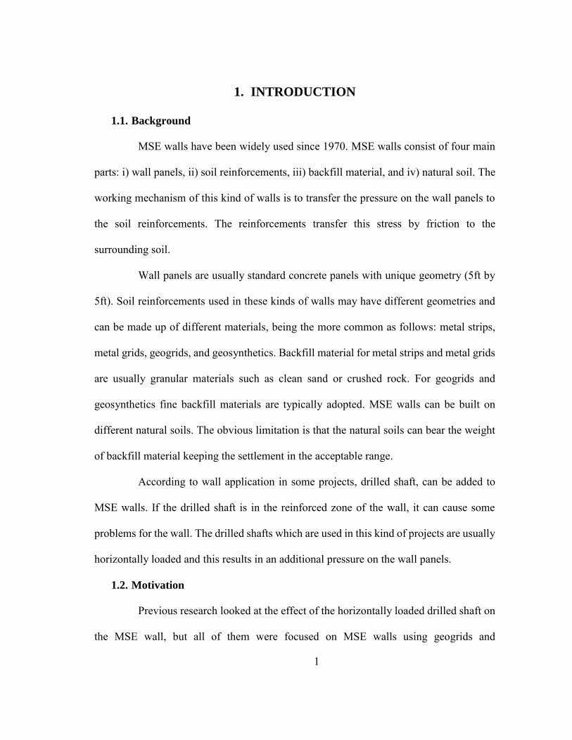
interrupted, laterally shifted or skewed as shown in Figure 2-5(b). The presence of the
drilled shafts affects also the compaction, particularly if the space between the drilled
shafts and MSE facing is limited. These problems associated with the presence of the
drilled shafts close to the on MSE wall could trigger some of the observed distresses.
17
(a) (b)
Figure 2-5 Conflict of shafts and reinforcement: (a) construction obstruction; (b)
rearrangement of reinforcement (Berg et al. 2009)
It was pointed out that the MSE wall could load the drilled shaft, this load can
be as a result of small movements of the MSE wall backfill, sliding and overturning of
MSE wall, reinforcement relaxation and seismic effects. However, no distress of drilled
shafts due to the imposed load from the MSE wall has been reported yet and no research
has been published either related to this problem.
2.3. Current research status
To properly address the interaction between drilled shafts/piles and MSE walls,
Kansas Department of Transportation (KDOT) and Utah Department of Transportation
(UDOT) have sponsored independent research programs (i.e. Pierson et al. 2008; Rollins
et al. 2010). These are the only published research on this topic. A summary of the KDOT
and UDOT research programs in this area is presented in Figure 2-6

18
KDOT Research
Objectives: To investigate the MSE wall resistance to the lateral load drilled shaft,
assess the possibility of using the resistance to shorten the required drilled shaft length
in the design, and develop general design guideline
MSE wall type: A 20’ high and 140 long’ geogrid reinforced modular block wall
Deep foundation type: Multiple drilled shafts of 36” in diameter
Research outline: The research encompassed of full-scale testing and numerical
modeling. The full-scale test examined the load-deflection of multiple drilled shafts,
which were of different length and located different distances from the MSE wall. The
load-deflection curves of the drilled shaft were developed. The numerical modeling
investigated the effects of different factor on the capacity of the shafts.
Outcomes: Ultimate capacity of multiple drilled shafts;
o Service limit considering different allowable deflection;
o The minimum spacing to avoid group effect;
o The effect of different factors (i.e., backfill material, reinforcement
and MSE wall facing unit) on capacity.
UDOT
Objectives: To investigate passive resistance of the backfill soil if a pile cap is loaded laterally and parallel to the length of the MSE wall. This loading condition would tend to occur during a seismic event. MSE wall type: Precast panel with metallic grids reinforcement
Deep foundation type: Driven piles with a cap.
Research outline: The pile cap was loaded laterally and parallel to the length of the wall under static, cyclic and dynamic loading conditions. The deflection and applied loads were monitored. Outcomes:
o Passive force-deflection curves; o Assessments of current methods used to develop the passive force-deflection
curve; o The performance of the MSE walls under such conditions.
Figure 2-6 Studies on the interaction between MSE walls and drilled shafts

19
2.4. Research outcomes of KDOT and UDOT research
2.4.1. KODT research
A 20-feet high and 140-feet long MSE test wall was built inside the southwest
clover of the I-435/Leavenworth road interchange in Kansas (Pierson 2007). The MSE
wall was a geogrid reinforced modular block wall. Multiple drilled shafts of a diameter
36” were built behind the MSE wall. The 120-feet long MSE wall was divided into 6 test
sections plus two wing wall sections at the ends as shown in Figure 2-7. Among 6 test
sections, one test section was 45-feet in width, which was designed to test a group of three
shafts situated at 72” from the MSE wall facing to investigate the group effect. Each of
the remaining 5 sections had one drilled shaft constructed behind it. Of the 5 test sections,
the drilled shaft was situated 36”, 72”, 72”, 108” and 144” away from the MSE wall facing.
One of two shafts situated 72” from the MSE wall facing was shorter than the rest, namely,
only that shaft had only 15” embedment depth into MSE wall backfill and the rest were
fully embedded (20’) into the MSE wall backfill. Each section was tested separately. Slip
joints were installed between the adjacent test sections to minimize the influence between
them. The MSE wall facing and drilled shaft were extensively instrumented with slope
inclinometers, LVDTs, tell tales, earth pressure cells, strain gauges, photogrammetry
targets to monitor (the deflections of the drilled shafts and the MSE wall facing), sensors
to measure the increases of the lateral earth pressure and geogrid strains (M. C. Pierson,
Parsons, Han, & Brennan, 2010).

20
Figure 2-7 Plan view of MSE test wall and shafts (Tensar 2007)
The shafts were laterally loaded by hydraulic jack towards the wall facing using
a displacement control mode as shown in Figure 2-8(a) and Figure 2-8(b). The load-
deflection curves of the shafts, including group shafts, were developed. Thereafter, a
numerical simulation was carried out to examine the influence on the capacity of the
drilled shaft of the following factors: different reinforcement types, quality of the backfill
material, and different MSE wall facing units.

21
Figure 2-8 Full-scale tests: (a) single shaft; and (b) group shafts
Based on the test data obtained, a design chart was developed as shown in Figure
2-9, which can be used to determine the drilled shaft capacity at the allowable deflection
and the given drilled shaft locations. Besides, an empirical equation was proposed to
calculate the minimum spacing between piles to avoid group effect as shown in Eq (2.1)
(Pierson 2010).
1 .4 7 6 .2 3in f lu e n c e w
W D (2.1)
Where Winfluence is the minimum spacing between shafts to avoid group effect [ft] and Dw
is distance from the MSE wall [ft].
A linear reduction factor was suggested, if the actual drilled shaft spacing is less
than Winfluence calculated from Eq (2.1). The reduced factor to account for the group effect
is shown in Eq (2.2).
(a) (b)

22
s in g le s
g ro u p
in flu e n c e
P SP
W (2.2.)
Where Psingle, Pgroup are the capacity of single and one group shafts respectively and Ss is
distance from the MSE wall [ft].
Figure 2-9 Design chart for drilled shaft
Numerical modeling of the interaction between the drilled shaft and MSE wall
have been carried out by Huang et al. (2011), Pierson (2010) and Pierson et al. (2011),
respectively. Based on the numerical modeling results, Pierson (2010) ranked the
influence of geogrid reinforcement, backfill material, MSE wall facing and height on the
drilled shaft capacity in descriptive terms, namely: high, medium and low. The only factor

23
rated with high influence was reinforcement. The other factors (i.e., backfill material,
MSE wall facing and height) have either medium or low effect on the drilled shaft
capacity.
2.4.2. UDOT research
When the bridge abutment is subjected to seismic acceleration, the piles can be
forced towards the backfill behind the abutment. The backfill behind the abutment may
be bounded by MSE walls on the sides as shown in Fig. 10. The load-deflection curve and
the performance MSE walls under seismic event are to be determined. The UDOT
research project was planned to: obtain the load-deflection curves; evaluate the current
design methods; and examine the effect of the passive force on the MSE wall.
The research encompassed one large-scale on the driven piles with a cap. The
illustration of the test setup is presented in Figure 2-10 and Figure 2-11. The pile cap was
loaded with two actuators, which were backed by two reaction shafts. The applied load
and the corresponding deflection were monitored. The passive force and deflection curve
was obtained and compared with current design methods as shown in Figure 2-12. In
addition, it was found that due to the effect of the loaded piles, the lateral earth pressure
in MSE wall could increase significantly, which could lead to excessive deflection or oven
failure. Pile cap deflection is shown in Figure 2-13.

24
Figure 2-10 Conceptual sketch of UDOT research (Rollins et al. 2010)
Figure 2-11 Test setup

25
Figure 2-12 Field tests (Rollins et al. 2010)
Figure 2-13 Passive force-deflection curves (Rollins et al. 2010)

26
2.4.3. Instrumentation of KDOT and UDOT research
The primary component of the field study is the monitoring program. Both
KDOT and UDOT research projects used extensive instrumentation for data acquisition.
The commonly used instrumentations are summarized in Table 2-1, which was used to
select the instrumentation used in this thesis as it is explained in the subsequent chapters.
The instrumentation in Table 2-1, except survey and LIDAR, has been used either in
KDOT or UDOT research projects. Survey and LIDAR, which is popular in remote
sensing, has been increasingly used to measure movement for engineering purpose (Laefer
et al., 2009).
Table 2-1 Commonly used instrumentations
Horizontal movement
Slope inclinometer
LVDT
Tell tale
Photogrammetry
Survey
String potentiometer
LiDAR
Strain Strain gauge
Earth pressure Earth pressure cell
Load Load cell

27
It has a few outstanding advantages such as remote monitoring. In the chapter 3
detailed comparison of the above instrumentation in terms of their advantages and
disadvantages will be discussed considering their application to this thesis research.
2.5. Other background information
Besides the published reports, papers, and presentations, communications with
engineers from different State Department of Transportation (DOTs) were maintained
during this thesis. The major pieces of information collected from the DOTs are:
None of the state DOTs have a rational design method to account for the interaction
between MSE wall and drilled shaft.
All engineers expressed interest in the investigation related to the interaction
between the MSE walls and drilled shafts. Most of the engineers considered that
such a research was important and necessary.
A few engineers considered that the interaction between MSE wall and drilled
shaft was a trivial issue, at least for the design at their state.
None of engineers were able to provide details of their practice on building MSE
wall with imbibed drilled shafts, including compaction details and any repair
measure for distressed MSE walls.
2.6. Conclusion
As it was discussed in this chapter, MSE walls are widely used to support bridge
abutment and in some cases, the interaction between the drilled shaft and the MSE wall
can be problematic. Some researches were performed on the interaction between MSE

28
walls with drilled shafts but soil reinforcements in these researches are geosynthetics and
geogrids. There is no proposed design guideline for these researches.
In this research the main focus is on the MSE wall with metal strips and metal
grids. A design guideline is proposed at the end to overcome the failure problem of MSE
walls with drilled shaft in the reinforced zone.
Instrumentation design for the full-scale test and two monitoring project sites
are discussed in the next chapter.

29
3. INSTRUMENTATION DESIGN
3.1. Instrumentation used in previous works
The First step of this Thesis research was the revision on previous works,
reported in Chapter 2. It was found that in recent years there were some other researches
somewhat similar to the one proposed in this Thesis, but the type of MSE wall
reinforcement used in this research and the tests protocols were quite different. The main
outcomes of these previous researches are practically not applicable to the MSE walls
project in Texas, because they do not involved metallic reinforcement (the most popular
reinforcement used by the Texas Department of Transportation for their design). In any
case these previous experiences have been very useful for this research, because it has
been possible to learn from them what kind of instrumentation worked well and adopted
it for the tests and monitoring contemplated in this Thesis. For example a total of seven
types of instrumentations were successfully used in the Kansas Department of
Transportation (KDOT) project, namely, strain gauges, earth pressure cells, load cells,
linear variable differential transducers (LVDTs), slope inclinometers, tell tales,
photogrammetry targets.
The strain gauges were installed to measure the strain developed in the
reinforcements. At each location the strain gauges were installed at the upper and lower
surface of the reinforcement to compensate for bending. To protect the strain gauges, they
were encased in a flexible plastic tube.
The earth pressure cells were installed to measure the increase of the earth
pressure induced by the laterally loaded drilled shaft. The installation adopted for the

30
earth pressure cells is shown in Figure 3-1. To provide an even surface between the MSE
wall facing block and the earth pressure cell, a masonry block was placed between the
earth pressure cells and facing wall, as shown in Figure 3-1. To protect the earth pressure
cell from compaction damage, a sand bag was placed between the earth pressure cell and
granular backfill material.
Load cells and LVDTs were installed at the head of the drilled shafts as shown
in Figure 3-2. The load cell was used to monitor the force applied at the head of the drilled
shaft. The LVDTs was installed to monitor deflection of the drilled shaft head. The LVTD
reading was used as a reference for the slope inclinometer readings since the bottom of
the slope inclinometer may have movements. The LVTDs was also installed to monitor
the relative movement between test shaft and reaction shaft (M. C. Pierson et al., 2009).
Figure 3-1 Installation of earth pressure cells (M. C. Pierson et al., 2009)

31
Figure 3-2 Installation of load cells and LVDTs (M. C. Pierson et al., 2009)
The tell tales were installed to monitor the movement of the backfill material
relative to the MSE wall facing. The tell-tale was arranged to measure backfill movement
in front of the drilled shaft and also surrounding the drilled shaft. The slope inclinometers
were installed at each test and reaction shaft and also at selected locations of the MSE
wall. The casing of the slope inclinometers was ended at the bottom of the drilled shaft.
Thus, the bottom of the slope inclinometers cannot be treated as a fixed end, since it may
move during the loading. The slope inclinometer readings were adjusted based on the shaft
head deflection provided by the installed LVDT (M. C. Pierson et al., 2009).
The MSE wall facing movement during loading was monitored by
photogrammetry. The photogrammetry targets are shown in Figure 3-3. Each target had a
6-inch long black portion, which provides reference for movement. A tripod was fixed
with a 10 megapixel digital single lens reflex (SLR) camera to capture the images of the

32
wall facing targets at designated time. The capture images were then restored into
AutoCAD. Using each target’s six inch scale, the MSE wall facing movement was
established by comparing the photo taken before and after each loading stage (M. C.
Pierson et al., 2009).
Figure 3-3 Installation of photogrammetry targets (M. C. Pierson et al., 2009)
In summary, a total of four different devices were used to monitor the deflection.
The advantages and disadvantage of these instrumentations are summarized in Table 3-1.
This discussion is based on the application of monitoring the drilled shaft behind MSE
wall. Thus, the conclusions may not be valid for other applications.

33
Load cell is used to monitor the applied load. It is important that the load cell
has in good contact with the monitored object. Since the load cell has certain dimensions,
an even and smooth contact surface is required. Strain gauges need to survive the
construction especially the compaction of the granular materials. Thus, protection
measure may be necessary.
Earth pressure cell needs to survive the construction as well. The earth pressure
cell relies on the good contact between backfill material and earth pressure cell. To obtain
reliable earth pressure monitoring data is a challenge, especially in granular materials. The
engineers always face the dilemma, namely, the compaction can easily damage the cells
and any protection measures for compaction may undermine the contact between the cell
and the backfill material.

34
Table 3-1 Comparison of different displacement monitoring instrumentations
Advantages Disadvantages
Slope inclinometer
Easy to implement Provide continuous profile Not susceptible to environmental deterioration Damage can be easily detected Easy to monitor multiple points on the same vertical line
Need a fixed end or reference point with known displacement Need access for monitoring personnel Need time to acquire each set of reading
LVDT Most accurate Need reference beams Costly if multiple points to be monitored
Susceptible for environmental deterioration Not suitable for long term monitoring Need access to the instrumentation
Tell tale Easiest to use Cheap
Least accurate Subject to construction damage Need access to acquire readings
Photogrammetry Easy to implement Low cost Time saving. Monitor multiple points at the same time No access to the monitored points is need. Can monitor the displacement from a distance away from the monitored objects
Need a scale reference Need clear view of the monitoring object Need photo process software to analyze the photo.
3.2. Adopted instrumentation
The final goal of the instrumentation is to gather experimental data that would
allow us to: better understand the problem; calibrate the numerical model; and ultimately
recommend guidelines. The actual site provides real world situation. The NGES site

35
affords the luxury of controlled loading conditions and the possibility for loading to
failure. For those purposes the following parameters were measured:
1- Deflection of drilled shafts.
2- Deflection of MSE wall panels.
3- Earth pressure at the back of MSE wall panels.
4- Earth pressure at the front of drilled shafts.
5- Strain in MSE wall reinforcement and in drilled shafts.
3.2.1. Shaft and wall deflection
To track the deflection of the shaft and wall panels, both inclinometer and
tiltmeter were used in this Thesis. On one hand inclinometer readings allow for a
continuous profile of the deflection at a certain time (time of reading). Because these
readings are generally taken manually, limited number of profile deflections are obtained.
On the other hand, tiltmeters provide an automatic and continuous monitoring of the wall
or shaft deflections but in a limited number of points (i.e. where the tiltmeters are placed).
In this research two tiltmeters were used on the shaft and other two on the wall. Deflections
of shaft and wall panels are an important parameter in numerical analysis, so it was
decided to use both inclinometer and tiltmeter for this project.
3.2.2. Earth pressure
It was needed to know the earth pressure at the back of the wall and in front of
the shaft. For this purpose, earth pressure cells were used. The backfill material used in
this research was clean sand and crushed rock. As explained above, they could cause some
problem for pressure cells resulting in not precise data. A type of pressure cells that is

36
working well with granular materials was adopted in this study. The working mechanism
and how it overcomes typical problems associated with earth pressure cells will be
discussed in the next Chapter. Pressure cells are installed at the top third of height the shaft
and wall.
3.2.3. Load in reinforcements
By measuring the strains in the wall reinforcement, its carrying can be
calculated. The strains can be measured using strain-gauges at specific positions of the
reinforcement. The total number of monitoring positions is limited by the number of
channels in data logger.
Preliminary numerical analyses (explained in Chapter 4) indicated that the force
in the reinforcement in the bottom 2/3 of the wall is small. So, all off strain gauges were
installed in the top 1/3 of the wall.
3.2.4. Data acquisition system
The experimental data provided from the different sensors is collected with a
data logger. Two data loggers were used for the full-scale test at the riverside tests. As for
the actual projects, only one data logger was used. The inclinometer was read manually.
Schematic sketches of instrumentation are shown in Figure 3-4 and Figure 3-5.

37
Figure 3-4 Schematic representation of instrumentation (plan view)

38
Figure 3-5 Schematic representation of instrumentation (cross section view)

39
3.2.5. Power supply
Power is needed for the data acquisition system. There was power supply at the
Riverside campus, however, this was not the situation at the two TxDOT actual sites and
solar panels were installed to provide the required power.
3.3. Adopted instrumentation
This section introduces all the instruments used in this research. They were
selected to measure displacements, deformations and stresses. For each instrument, a
general description is presented, followed by their main advantages and disadvantages.
Afterwards, the data acquisition system and communication system is presented
respectively.
For all the electronic devices that can be used in this research, there are two
different functional systems that can be selected. The traditional one, also known as a
voltage based system, and a relatively new system which is based on vibrating wires.
In the traditional one, the parameters to be measured are relayed via the gauge
base (electrical insulation) to the resistance wire or foil in the gauge. As a result, the fine
wire (or foil) experiences a variation in electrical resistance. This variation is exactly
proportional to the parameter. For example a strain-gauge is constructed by bonding a
fine electric resistance wire, or photographically etched metallic resistance foil, to an
electrical insulation base using an appropriate bonding material, and attaching the gauge
leads.
In the vibrating wire system, the resonant frequency of vibration of a tensioned
steel wire is dependent on the strain or tension in the wire. This fundamental dependency

40
is utilized in a variety of configurations for the measurement of strain, load, force,
pressure, temperature, and tilt. Vibrating wire sensors are well known for their long-term
stability. The advantage of vibrating wire sensors over more conventional types mainly
lies in the sensor output, which is a frequency rather than a voltage. Frequencies can be
transmitted over long cables (i.e >2000 m) without appreciable degradation of the signal
caused by variations in cable resistance, which can arise from water penetration,
temperature fluctuations, contact resistance or leakage to ground. This factor designs
results in sensors which exhibit good long-term stability and which are convenient for
long-term measurements in adverse environments.
In this Thesis it was decided to use instruments based on the conventional system
(i.e. voltage base system). Different reasons supported this decision, some of them are
discussed as follows. Vibrating wire is a relatively new method, the majority of the
previous projects undertaken at TAMU were instrumented with sensors based on the
voltage method. Therefore, technicians are more familiar with this method. The price for
instrumentations based on vibrating wires is much higher. In some cases it is about three
or four times higher than the conventional types. It is also recommendable to use a single
method for all of the devices in a particular project. Otherwise, two (or more) separate
data acquisition systems will be necessary, (i.e. for the voltage based gauges and another
for the vibrating wire ones). To use two different kinds of data acquisition systems in a
single project is not recommended.

41
3.3.1. Tiltmeter
The tiltmeter is an instrument used for measuring inclination. It output is
determined by the mass distribution of the earth, since it responds to the local acceleration
of gravity (g). This instrument is sometimes called inclinometer, particularly if its range
of reading is large. The response of the instrument is determined by the direction of g
relative to its orientation.
Figure 3-6 Tiltmeter used in the project
The principles of operation can be illustrated with common tools of carpentry.
Consider a static plumb-bob, which would constitute a spherical pendulum if the system
were dynamic. The plumb-bob orients itself along the direction of g, and thus defines the

42
local vertical. Alternatively, a fluid bubble, contained by a tube, will determine one of the
locus of directions, orthogonal to g, which constitute the local ``level". The tiltmeter used
in this project is shown in Figure 3-6.
3.3.2. Inclinometer
It is a device to measure angle of a slope. In this project it is going to measure
vertical deflections of wall and the shaft.
There are many differences between an inclinometer and a tilitmeter. Perhaps
the more relevant ones is that an inclinometer gives the deformation profile at a specific
time (i.e. at the end of the reading) for the whole depth of the inclinometer casing. In
contrast, the tiltmeter gives the deflection at a specific point but for the whole time of
analysis, allowing continuous monitoring.
The main components of an inclinometer are discussed as follows.

43
Figure 3-7 Inclinometer
3.3.2.1. Components of a portable inclinometer system
Inclinometer casing: the inclinometer casing is permanently installed in a
borehole that passes beside the wall and shaft.
Portable traversing probe: the traversing inclinometer probe is the standard
device for surveying the casing. It is economical, since it can be carried from site to site.
The traversing probe obtains a complete profile because it is drawn from the bottom to the
top of the casing.

44
Portable readout: a portable readout is used to record the surveys obtained with
the portable probe. Advance readouts store readings in solid-state memory, eliminating
pencil, paper, and transcription errors, and transferring the data to a computer for their
processing.
The main components of the inclinometer device are presented in Figure 3-7.
3.3.2.2. Calibration
The existing inclinometer was calibrated following the protocol indicated by the
manufacturer company (Slope Indicator). First the casing was placed in an approximately
vertical position. Then the probe was inserted into the casing and the initial inclination
was read. Then, a known displacement was applied to the top of the casing maintaining
fix the bottom of the casing. A new reading was taken with the inclined casing. Then, by
a simple calculation, the change in the angle was obtained. In this way the change in the
reading could be easily related to the change in the angle. For a more precise calibrating
factor, the procedure can be done using more points.
The calibration factor for the existing inclinometer is 0.297. The inclinometer
was calibrated each three months.
3.3.3. Photogrammetry
Photogrammetry may be defined as a technique used to obtain reliable
information from physical objects and the environment. This is done through a process of
recording, measuring, and interpreting aerial and terrestrial photographs. In a sense, the
word photogrammetry may be analyzed in two parts: photo - meaning "picture," and
grammetry - meaning "measurement."

45
The fundamental principle used by photogrammetry is triangulation. By taking
photographs from at least two different locations (the so-called "lines of sight"), it can be
developed from each camera to points on the object. These lines of sight are
mathematically intersected to produce the three-dimensional (3D) coordinates of the
points of interest (Figure 3-8).
Figure 3-8 Photogrammetry
3.3.4. Pressure cells
Earth pressure cells, sometimes also called total pressure cells or total stress cells
are designed to measure stresses in soils, or the pressure of soil on structures. Pressure
cells will respond not only to soil pressures but also to ground water pressures or to pore

46
water pressure. Hence the term total pressure or total stress is appropriate. In this project,
we do not anticipate the presence of pore water pressure, so the output is the soil pressure
only.
From previous works, it was observed that when dealing with granular material,
it was very hard to obtain reasonable results from pressure cells. In this Thesis special care
was taken to gather good results from this instrument. This is explained later on chapter
4.
The earth pressure cells described here are of the hydraulic type. In which two
flat plates are welded together at their periphery and are separated by a small gap filled
with a hydraulic fluid. The earth pressure acts tending to squeeze the two plates together,
building up the pressure inside the fluid. If the plates are flexible enough (i.e. if they are
thin enough relative to their lateral extent), then at the center of the plate the supporting
effect of the welded periphery is negligible and it can be stated that at the center of the cell
the external soil pressure is exactly balanced by the internal fluid pressure.
3.3.5. Strain gauges
Strain Gauges are widely used for physical force measurements in mechanical,
marine, aircraft and civil engineering as well as the fields of architecture, automobiles,
and medical science. Strains are measured to determine the degree of deformation induce
by the mechanical loads. By knowing the elastic modulus of the material under study it is
possible to determine the stress and also the forces acting in the instrumented element.

47
There are a number of ways of measuring strain mechanically and electrically,
but the vast majority of stress measurement is carried out using strain gauges due to their
superior measurement characteristics.
External force applied to a material generates physical deformation and
electrical resistance change of the material. In case that such material is stocked onto test
specimen via electrical insulation, the material produces a change of electrical resistance
corresponding to the deformation. Strain gauges consist of electrical resistance material
and measure proportional strains to the resistance changes.
When strains are generated in a test specimen, and a strain gauge is attached to
it, the strain is relayed via the gauge base (electrical insulation) to the resistance wire or
foil in the gauge. As a result, the fine wire (or foil) experiences a variation in electrical
resistance that is proportional to the strain. Vibrating wire strain-gauges work based on
the principle explained above.
There are many different manufacturers and different models of foil strain-
gauges. The main differences between them are related to the way in which they are glued
on the surface. The lead wire can be preinstalled or not and also may have different range
of electrical resistance. According to the experience from previous projects at TAMU, in
this Thesis the gauges code as TML-FLA-5 was chosen.
3.3.5.1. Calibration
The first step for installing a strain gage is to clean the surface and make it
shining by using sandpaper. Figure 3-9(a) and Figure 3-9(b) shows the main initial steps
followed to glue the strain-gauge to the metallic strips used in this thesis. First a coarse

48
sand paper was used to prepare the surface and then progressively finer ones were used to
polish the strip surface. When the strip surface was clean and polish, acetone was applied
for the final treatment.
(a) (b)
Figure 3-9 Clean the strip surface by sand paper
Once the surface was ready, the strain gage was placed on the target position
and a band tape was used to provisionally fix it. Then some super glue was put on the
target position and the strain gage was rolled back to it (Figure 3-10)

49
Figure 3-10 Installed strain gauges
Once the strain gauge was installed, the lead wires were connected to the data
logger. Then one side of strip was fixed and some weights were applied on the other end,
as shown in Figure 3-11. The weights were applying in steps. The maximum was 46.7
grams. The strip was then unloaded. By knowing the strip material and its modulus of
elasticity, the strain gauges could be easily calibrated.
50
Figure 3-11 Testing strip with strain gauges
The gauge factor 2.11 was tested (the one in the catalog). As it is shown in Figure
3-12, the results are acceptable.

51
Figure 3-12 Calibration results
3.3.6. Data acquisition system
The data acquisition system is used to read the data from the instruments and
save them. The main components of this system are: data logger, solar panel, and battery.
They are introduced below.
3.3.6.1. Data logger
The data logger adopted in this project is a Campbell Scientific CR1000 (Figure
3-13). The experience at TAMU in previous projects with this type of system was very
good, because of this was selected in this Thesis.
Some of the benefits of this device are:
Serial communications with serial sensors and devices supported via I/O port pairs.
It supports all of devices used in this project.
0.00E+00
5.00E-08
1.00E-07
1.50E-07
2.00E-07
2.50E-07
0 10 20 30 40 50
stra
in
weight (kg)
theory
Test

52
Compatible with channel expansion peripherals allowing the expansion of the
system. By default, it has 16 channels. It is possible to expand it to 32 if necessary.
Figure 3-13 CR1000 data logger
3.3.6.2. Solar Panel
In this Thesis for power supply Campbell Scientific SP10-10W solar panel was
used (Figure 3-14). It supplies electrical power in locations where AC power is unreliable,
expensive, or not available.

53
3.3.6.3. Battery
Campbell Scientific PS100 rechargeable power supply was used in this Thesis
(Figure 3-15). The PS100 provides a 12-Vdc, 7-Ahr rechargeable power supply. The
rechargeable battery can be trickle-charged from ac or from an external solar panel.
Figure 3-14 SP10-10W solar panel
Figure 3-15 PS100 rechargeable power supply

54
3.4. Conclusion
Instrumentation design was performed based on the required information from
full-scale test at Riverside campus and the monitoring from two actual sites. The most
important limitation was the number of channel in the data logger. For the full-scale test
two data loggers were used and totally 20 channels were collecting data. For the
monitoring at actual sites one data logger used for each site and 15 channels were
collecting data.
Types of devices were selected according to the required precision and
durability. Durable devices were needed especially for monitoring actual sites, because
they were designed to collect data for one 16 months.
Full-scale test and monitoring of actual sites are discussed in detail in next
chapter.

55
4. FIELD STUDIES-TESTS AND MONITORING
4.1. Introduction
This chapter focuses on the monitoring and testing of the MSE wall at the field
sites. Monitoring was planned for two actual sites selected by TxDOT and the load test
carried out at the National Geotechnical Experimentation Site (NGES) at Texas A&M
University. One of the actual project selected by TxDOT is in Bastrop. This project was
finished in December 2013 and data is being collected from this time since now. The
second actual project selected by TxDOT is in Salado. This project was delayed and no
data was collected from this project yet.
At NGES a full scale loading test was carried out on a new MSE wall. The aim
of this experiment was to study the interaction between the drilled shaft and the MSE wall
under actual conditions. The drilled shaft, MSE wall and other components used during
the loading test were designed and constructed by TTI (Texas A&M Transport Institute)
researchers and under the supervision of the Ph.D. candidate and his supervisors. The
instrumentation used to gather all the data required by this research was designed and
installed (as explained in the previous Chapter) by the Ph.D. candidate with the help and
supervision of his supervisors and TTI researchers. The loading protocol was proposed by
the candidate and supervisors and aggraded with TxDOT personnel.
The main objective of this research is to study the interaction between drilled
shafts subjected to horizontal loads and MSE walls. In particular the research interest
focuses on the effect of the applied horizontal load (on the drilled shaft), particularly on:
drilled shaft displacement,

56
wall displacement,
additional pressure on the wall, and
additional force developed in the soil reinforcements and their distributions in
different positions
This chapter is organized as follows: Section 3.2 is related to the full scale test
at NGES. It also introduces details associated with the wall and the drilled shaft, materials;
and also the devices used for gathering the data. The loading protocol, test preparation,
performance and results are discussed in this section. Section 3.3 deals with the real MSE
wall at the Bastrop monitoring site, describing the installation of different devices on the
wall and drilled shaft. The data collected from this site is also presented in this section.
Section 3.4 is related to the other real site in Salado and the work progress at that site.
4.2. Full-scale loading test
4.2.1. Overview
This part focuses on the different components of the loading test. Section 3.2.2
presents the wall details. Section 3.2.3 deals with the backfill material. Section 3.2.4
presents the reinforcement used in this test (metallic strips) and the corresponding
instrumentation. The design of the drilled shaft is presented in Section 3.2.5. The different
devices used in this research to gather the experimental data are discussed in Section 3.2.6.
Section 3.2.7 deals with the construction of the wall. The description of the loading
protocol and test results are presented in section 3.2.9. Finally, Section 3.2.10 presents a
short discussion about the results obtained in the loading test.

57
4.2.2. Wall detail
The test was carried out in a new MSE wall constructed in the Riverside
Campus. This wall was part of a much longer wall built in the context of a NCHRP project
aimed at studying the impact of a tractor trailer on the wall. This NCHRP project includes
conducting a full scale crash test of an 18 wheeler tractor-trailer against an “L shape
barrier” placed at the top of the MSE wall as shown in Figure 4-1. The length of the wall
is 90 ft and its height is 7.5 ft.
Figure 4-1 Wall detail
The panels for the wall were donated to the project by the company Reinforced
Earth Company (RECO). Each panel has 6 ties for strips (2 rows and 3 columns). The
height of panel is 4’10”. The designed height of wall was achieved by using one and a half
panels. Detail of the panel is shown in Figure 4-2.

58
These panels are not designed for lateral pressure of soil or additional pressure
caused by horizontal load of drilled shaft, the minimum reinforcement is used to contract
them (R. R. Berg et al., 2009).
A foundation to transfer the vertical load from the panel to the soil needs to be
constructed in this kind of project (R. R. Berg et al., 2009). Usually the foundation is made
from low strength concrete or wood. In this project the foundation was from wood.
Figure 4-2 Panel details

59
4.2.3. Backfill material
The backfill material used in this test program was a fine to medium sand. This
sand satisfies the requirements for MSE select backfill specified in AASHTO (American
Association of State Highway & Transportation Officials. Subcommittee on Bridges,
2010). Particle size distribution curve for the MSE wall backfill material used in the full
scale test is shown in Figure 4-3
Figure 4-3 Gradation curve for backfill material

60
The strength parameters of the backfill material were determined via three
triaxial tests type CD (i.e. Consolidated-Drained) performed by the candidate. Those tests
were performed at 3 different confining pressures, which were selected according to the
depth of the instrumented strips adopted in this research. Test results for a confining
pressure (σ3=σ2, both horizontals stresses) of 7 KPa is shown in Figure 4-4 and Figure 4-5.
Results for a confining pressure of 14 KPa are shown in Figure 4-6 and Figure 4-7, and
results for a confining pressure of 31 KPa are presented in Figure 4-8 and Figure 4-9.
Triaxial result is shown in Figure 4-10.
To determine the strength properties of the fill, the tests results have been plotted
in the “s-t” space as follows: s = (σ1+σ3)/2 and t = (σ1-σ3)/2. Figure 4-11 presents the main
results. To determine the friction angle, it should be considered that sin (φ) = tan (α) and
for cohesion c = a/cos(φ) (Holtz, Kovacs, & Sheahan, 2010).
The friction angle for backfill material is 27.3° and the cohesion is 5.45 KPa
ta n ( ')
' ( ) ta n ( ')
ta n ( ') 1 0 .5 6
a p p
w
a p p w w
c
c u
c u u K P a
Figure 4-4 Stress-strain curve for σ3=7KPa
0
5
10
15
20
25
30
0 2 4 6 8 10 12 14 16
q(K
Pa)
εa

61
Figure 4-5 Volumetric strain vs. axial strain for σ3=7KPa
Figure 4-6 Stress-strain curve for σ3=14KPa
Figure 4-7 Volumetric strain vs. axial strain for σ3=14KPa
-2.5
-2
-1.5
-1
-0.5
0
0.5
0 2 4 6 8 10 12 14 16εv
εa
0
10
20
30
40
50
0 5 10 15 20
q (
KP
a)
εa
-3.5
-3
-2.5
-2
-1.5
-1
-0.5
0
0 5 10 15 20
εv
εa

62
Figure 4-8 Stress-strain curve for σ3=31KPa
Figure 4-9 Volumetric strain vs. axial strain for σ3=31KPa
0
20
40
60
80
0 5 10 15 20
q (
KP
a)
εa
-4
-3
-2
-1
0
0 5 10 15 20
εv
εa

63
Figure 4-10 Triaxial result for backfill material
Figure 4-11 Results in s-t plain
y = 0.458x + 4.8523R² = 0.9911
0
5
10
15
20
25
30
35
40
0 10 20 30 40 50 60 70
t (K
Pa)
S (KPa)

64
4.2.4. Wall reinforcement
The reinforcements used in this study are metal strips. Detailed specifications of
strips are shown in Figure 4-12. They were provided by RECO. The strips used in this
project are shown in Figure 4-13.
Figure 4-12 Details of metal strip (The Reinforced Earth Company 2005)
Not to scale

65
Figure 4-13 Photos of the trips provided by RECO
4.2.5. Drilled shaft
The length of the drilled shaft is 17.5 ft., where the total length is distributed as
follows (Figure 4-14(a)): 7.5 ft. in the natural soil; 7.5 ft. imbibed in the back fill material,
and 2.5 ft. above the back fill level (this portion is necessary to apply the horizontal load.
As indicated in Figure 4-14(b), the diameter of the drilled shaft is 2 ft. The rebar details
are shown in the same figure.
As shown in Figure 4-1, the distance between the center of the drilled shaft and
the edge of the wall in the “southern part” was 17.5 ft. The drilled shaft was placed in a

66
position in order to have a full panel on top and a half panel in the bottom (in front of the
drilled shaft).
(a) (b)
Figure 4-14 Drilled shaft detail
4.2.6. Instrumentation
To gather all the information from the test, there were instruments installed on
the wall and other ones installed on the drilled shaft. Table 4-1 summarizes the
instrumented used in this project. It also presents the parameter to be measured and the
location of the instrumentations.

67
Table 4-1 List of instruments used in the project
What to Measure Device Wall Drilled shaft
Horizontal movement
Photogrammetry Yes No
Survey Yes Yes
Inclinometer Yes Yes
tiltmeter Yes Yes
String potentiometer Yes Yes
Stress Strain gauge Yes No
Earth Pressure Earth pressure cell Yes Yes
Load Load cell No No
4.2.6.1. Strain Gauge
Strain gauges are installed on the strips to measure the force transfered to them
during the application of the horizontal loads. The stresses to be measured are the axial
force in the strips. Therefore the strain-gauges are installed in a way that the stresses that
may be generated due to bending and/or temperature changes are compensated. To
compensate these spurious stresses, a full bridge circuit containing the four strain gauges
has been adopted for each position.
The previous step, before installing the strain gauges, was to smooth the strips
surfaces in all the positions were gauges needed to be glued. A rotating machine with

68
sandpaper was used for this purpose, as shown in Figure 4-15. The surface should be clean
and shiny, like a mirror (Figure 4-16).
Figure 4-15 Rotating machine with sand paper
Strain gauges and the corresponding connectors were installed using super glue,
as it is shown in Figure 4-17. The connectors were used to install extended wires. For
protecting the strain gauges and connectors PVC tape was wrapped around them (Figure
4-18).

69
Figure 4-16 Clean and shiny surface
Figure 4-17 Strain gauge and connector installed using super glue

70
Figure 4-18 Protecting strain gauges and connectors using PVC tape
4.2.6.2. Tiltmeter
Tiltmeters were used to gather the deflection of the wall and drilled shaft (Figure
4-19). Two tiltmeters were installed on the drilled shaft and the other two on the wall.
They were installed at the same level in both structures (i.e. on drilled shaft and wall) to
enable comparisons of deformation. They tiltmeters were placed inside aluminum boxes
to protect them from any damage during wall construction (Figure 4-20). The tiltmeters
were oriented in a way that they can measure the deflection perpendicular to the wall.

71
Figure 4-19 Tiltmeter used in this project
Figure 4-20 Aluminum box used to protect tiltmeter

72
4.2.6.3. Pressure Cell
Two pressure cells were used in this test. One of them was installed on the wall
and the other one on the drilled shaft. These kinds of devices rarely work well in previous
projects reported in the literature dealing with sand and gravel as fill material. To
overcome this problem, two main decisions were taken in this project:
Relatively larger and more precise pressure cells than the ones generally
adopted in other projects were adopted in this project (Figure 4-21). They
have a big diameter (8 in) in order to prevent arching which normally
occurred in sand. . They were also quite expensive (more than 1600$
each cell).
Special care was taken during the placement and compaction of the soil
around the cell. This is to prevent typical problems observed at the
contact between the sand and the pressure cell. To solve this problem,
the soil between two pressure cells was compacted manually in small
layers (i.e. around 4 in each), as shown in Figure 4-22.
Pressure cells were installed at the top the wall and drilled shaft. The distance
between center of pressure cells and top of the wall was about 10 inches. Because the load
was applied at top of the drilled shaft, it was anticipated that the maximum pressure will
be induced at top part of the wall.

73
Figure 4-21 Pressure cell used in the test
Figure 4-22 Manually compacted area between two pressure cells

74
4.2.6.4. Inclinometer
In addition to tiltmeters, inclinometer was used in this test for measuring wall
and drilled shaft deformation (Figure 4-23). On one hand the inclinometer provides the
whole profile of deformation (i.e. in the total length analyzed, in the wall or drilled shaft)
at given times (i.e. when the measurements with the inclinometer probe take placen). On
the other hand the tiltmeters provide continuous information in time, but for the punctual
position in which the device is installed. So, to have complementary information of the
deflections in this Thesis it was decided to use both of them.
Figure 4-23 Inclinometer probe
When doing the measurements with the inclinometer, the probe (Figure 4-23)
should go through a plastic casing and the data is read at pre-established depths. The

75
plastic casings needed to be installed in advance. An important aspect of this technique is
to have a good zero (i.e. a reference) reading for the deflections. This is achieved by
installing the casing up to a depth that there is not deflection (i.e. reference for the
measurements). In this project, casing for the wall went in natural soil (under the wall)
one time of wall height (7.5 ft). For the drilled shaft, it went only 3 ft. (Figure 4-24) below
the bottom of the drilled shaft. This was due to drilling constrains. The candidates and
advisors consider that this depth can be enough for this study. In any case, the readings
were studied to check whether this is a good zero for the measurements.
Figure 4-24 Detail of the casing

76
4.2.6.5. Photogrammetry
Photogrammetry was used to track the wall deformation. The procedure is very
simple. 30 signs were installed on the wall as shown in Figure 4-25. On each sign a mark
of exactly 4 inches (10 cm) in black was included. During the loading test, after each load
step, a camera was used to take pictures of the wall with those signs on the wall face. A
key aspect is that the camera cannot be moved during the test. To ensure that the camera
is fix; a remote device should be used for capturing the photos. This will prevent any small
movements that may be induced by the operator during capturing manually the photo from
the main camera.
Figure 4-25 Photogrammetry signs

77
For each load step and each sign there are couples of pictures that can be
compared with the initial state of wall to get the deformation of the targets points.
To process the photos, the main steps below have to be followed:
1- Take the initial picture (t=0) to the CAD and make it first layer.
2- By using image processing pieces of software (like Photoshop) target photo
can be made transparent.
3- Take that picture to CAD and study a second layer.
4- Measure the movement of the signs.
5- Compare the movements with known length of the black part (4 in) and
calculate the movements.
The signs were made of 3 inch PVC tubes (Figure 4-26). For installing them on
wall, PVC floor drains were used (Figure 4-27). A sample photo used for the
photogrammetry study is shown in Figure 4-28.
In order to be sure that temperature and sun shine did not affect signs, a number
of control signs, installed on a far end of the wall, were used as reference. The length was
measured before and after the test. The length was exactly the same, which indicate that
the dilation to the temperature had practically no impact on the results.

78
Figure 4-26 PVC tube used for photogrammetry
Figure 4-27 Floor drain used to install PVC tubes on the wall

79
Figure 4-28 Sample photo that used for photogrammetry
4.2.6.6. Spring Pot
String pots were used to measure the absolute displacement of the top of the
drilled shaft respect to the top of the wall. The string pot used in this project is shown in
Figure 4-29.
A fixed point was needed to attach one end of string pot to it (i.e. The reference
point). A metal rod was installed 14 ft away from the wall to make sure it wouldn’t move
during the test. The other end is attached to the drilled shaft. Another string pot was used
between the drilled shaft and the wall (Figure 4-30)

80
Figure 4-29 String pot used in this project
Figure 4-30 Fixed point and string pots
4.2.6.7. Loading
To apply load to the drilled shaft a hydraulic jack (see Figure 4-31) and pump
were used (see Figure 4-32). The jack capacity was 100 kips and the maximum allowed
movement of the treaded rod in the jack was 6 inches.

81
Figure 4-31 Hydraulic jack
Figure 4-32 Pump for hydraulic jack
For the application of the load, a pulling system was designed. So, the pulling
frame was installed in front of the wall on the pavement (Figure 4-33(a)). Another loading
frame was installed on the drilled shaft (Figure 4-33(b)).

82
(a) (B)
Figure 4-33 Load frame on (a) the pavement (b) the drilled shaft
Load frames (both on the drilled shaft and on the pavement) were designed for
a maximum force of 100 kips. Details of the frames and their locations in the relative
position in the test setup are shown in Figure 4-34.
4.2.7. Construction of the wall
The first step for constructing the wall was the excavation (Figure 4-35). As
mentioned before, the height of the wall was 7.5 ft.; therefore the bottom of the excavation
was set to achieve the required wall elevation. Slope for the dig was 45 degree in all
directions.

83
Figure 4-34 Details of loading frames
Figure 4-35 Excavation

84
Once the excavation was completed, it was time for constructing the foundation
of the wall, as shown in Figure 4-36. One important aspect for this project was to leave an
empty space in the foundation (before pouring the concrete) for the inclinometer casing,
in the exact position where the inclinometer readings wanted to be taken.
Once the foundation was finished the installation of the panels started. The
panels were installed in rows and they were held by means of wood brackets. Figure 4-37
presents how the panels were kept vertical until the reinforcements and fill were placed.
Figure 4-36 Wall foundation

85
Figure 4-37 First rows of panels
The drilled shaft was constructed just after the excavation was completed and
before the wall (Figure 14). The casing for inclinometer in the drilled shaft was placed
with the rebar cage as shown in Figure 4-38.
Once the first row of panels was placed the backfill material was compacted.
The sand was poured behind the panels and compacted until the level reached the first
layer of strips (Figure 4-39). Then as it is shown in Figure 4-40, strips were placed and the
installation continued by layers following the same procedure for the other levels of
reinforcements.

86
Figure 4-38 Drilled shaft behind the wall
Figure 4-39 First layer compaction

87
Figure 4-40 Installed strips (first layer)
.
4.2.7.1. Compaction
The backfill was compacted in loose lifts of 6 in. (152.4 mm) to 12 in. (304 mm)
thick maximum with 6 passes of a 2,176 lb (9.7 kN), 35 in. (890 mm) wide drum roller.
The maximum dry density of the backfill was 117.8 pcf (18.5 kN/m3), this value was
determined by the modified compaction Proctor test.
Two nuclear density tests were conducted at the level of the bottom layer of the
strips (Figure 4-41). The average dry density and water content were 111.7 pcf (17.5
kN/m3) and 3%, respectively. This dry density represents 95% of the maximum dry density
obtained in the modified Proctor test for the backfill material (ASTM D1557-12, 2000).
The compaction curve is presented in Figure 4-42

88
Figure 4-41 Nuclear density test
Figure 4-42 Compaction curve
95
100
105
110
115
120
125
0 2 4 6 8 10 12
Dry
uni
t wei
ght (
pcf)
Water Content (%)

89
4.2.8. Loading test
The loading test was carried on Wednesday 22nd August 2012. It started at 10:45
AM and was running for 3 hours (Figure 4-43)
Figure 4-43 Photo taken during the load test
Due to the large amount of data gathered during the loading test two data loggers
were necessary. The main data logger was provided by the local TTI team at NGES and
the other one was bought for this Thesis.
All of the instruments, but the tiltmeters were connected to the main data logger
(NGES one). In total 20 channels were used to read the data collected during the test each
30 seconds. The data associated with the inclinometer, it was read manually after each
load step. Figure 4-44 Shows different key positions associated with the load test.
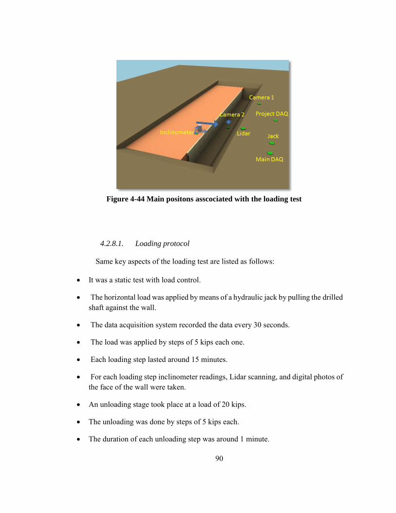
90
Figure 4-44 Main positons asscociated with the loading test
4.2.8.1. Loading protocol
Same key aspects of the loading test are listed as follows:
It was a static test with load control.
The horizontal load was applied by means of a hydraulic jack by pulling the drilled shaft against the wall.
The data acquisition system recorded the data every 30 seconds.
The load was applied by steps of 5 kips each one.
Each loading step lasted around 15 minutes.
For each loading step inclinometer readings, Lidar scanning, and digital photos of the face of the wall were taken.
An unloading stage took place at a load of 20 kips.
The unloading was done by steps of 5 kips each.
The duration of each unloading step was around 1 minute.
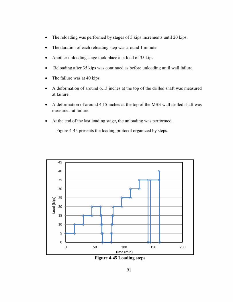
91
The reloading was performed by stages of 5 kips increments until 20 kips.
The duration of each reloading step was around 1 minute.
Another unloading stage took place at a load of 35 kips.
Reloading after 35 kips was continued as before unloading until wall failure.
The failure was at 40 kips.
A deformation of around 6,13 inches at the top of the drilled shaft was measured at failure.
A deformation of around 4,15 inches at the top of the MSE wall drilled shaft was measured at failure.
At the end of the last loading stage, the unloading was performed.
Figure 4-45 presents the loading protocol organized by steps.
Figure 4-45 Loading steps
0
5
10
15
20
25
30
35
40
45
0 50 100 150 200
Load
(ki
ps)
Time (min)

92
4.2.9. Main results associated with the loading test
The results gathered during the test can be organized in different ways. In the
following sections some relevant plots combining the more relevant information are
presented to assist the interpretation of the experiment during the load test and to learn
about the behavior of the drilled shaft and main components of the wall.
4.2.9.1. Load-Displacement curve
One of the main goals of the test was study the displacement of wall and drilled
shaft observed during the different horizontal load steps. Maximum deformation of wall
occurred in front of the drilled shaft. String pots were used to measure the maximum
deformation of both: drilled shaft and wall. The load-displacement curve for drilled shaft
is shown in Figure 4-46. The maximum deformation of drilled shaft was 6.13 inches and
took place at the horizontal load of 40 kips. At that load, the maximum deformation of
wall was 4.15 inches. This is presented in Figure 4-47.
Figure 4-48 presents the displacement of the drilled shaft against the wall
displacement. As expected, drilled shaft deformation is greater than wall deformation in
all the steps. The difference between these two movements is related to the soil
compression.

93
Figure 4-46 Load-displacement for drilled shaft
Figure 4-47 Load-displacement for wall
0
5,000
10,000
15,000
20,000
25,000
30,000
35,000
40,000
45,000
0.0 1.0 2.0 3.0 4.0 5.0 6.0 7.0
Load
(lb
)
Displacement at top(inch)
drilled shaft
0
5,000
10,000
15,000
20,000
25,000
30,000
35,000
40,000
45,000
0.0 0.5 1.0 1.5 2.0 2.5 3.0 3.5 4.0 4.5
Load
(lb
)
Displacement at top (inch)
Wall

94
Figure 4-48 Plot showing the drilled shaft against the wall displacement
4.2.9.2. Stresses in strips
Other very relevant results obtained from the test were the stresses developed in
the strips during loading. As mentioned before, in MSE walls all of horizontals loads are
taken by the strips. Strain gauges were used to measure the stresses in the strip. There were
6 instrumented strips in the upper part of the wall, in the two top rows of strips. One of the
instrumented strips had 4 strain gauges (S-4-1). Two of them had 2 strain gauges(S-2-1 &
S-2-2) and three of them had only 1 strain gauge (S-1-1, S-1-2 & S-1-3). The positions of
those strips (as coded) are shown in Figure 4-49. The selection of the instrumented strips
and the distribution of the gauges along them were based on a numerical modeling
performed before the test and aimed at designing the instrumentation. For example, the
model predicted that the forces in the second layer of strips were higher than the ones in
0
1
2
3
4
5
6
7
0 1 2 3 4 5 6 7
Dril
led
shaf
t dis
plac
emen
t (in
)
Wall Displacement (in)
Data
45 degreeline

95
the top layer. Accordingly, the strips with more instruments were located in the second
layer. The strip with 4 gauges was instrumented to learn about the distribution of stresses
along the strip.
The results associated with forces in strips are presented grouped in 2
categories: forces in the strip developed due to the geostatic force only; and forces
developed due to the horizontal load applied to the drilled shaft only (i.e. without geostatic
effects). The case without geostatic is for studying the effect of lateral load only on the
strips.
Figure 4-49 Strips numbers and positions
As mentioned before, the strip with more instruments is the one with 4 gauges
(S-4-1). Positions of strain gauges are shown in Figure 4-50.

96
Figure 4-50 Strip with four strain gauges (S-4-1).
Figure 4-51 presents the forces developed in strip S-4-1 for the different
positions in the strips and load steps considered in the tests. As expected, the force in the
strip decreases with the distance from the wall. It is interesting to see that the maximum
force in the strip does not occur at the maximum horizontal load applied to the drilled
shaft. In this case the maximum force in the strip is 3.86 kips and it occurred at the
horizontal load of 25 kips.
Figure 4-52 presents the forces in the strips including geostatic forces. In this
case the maximum force in the strip was 4.7 kips.

97
Figure 4-51 Force in the strip S-4-1 excluding Geostatic force
Figure 4-52 Force in the strip S-4-1 including Geostatic force
0
500
1,000
1,500
2,000
2,500
3,000
3,500
4,000
4,500
0 20 40 60 80 100 120
Forc
e (
lb)
Distance from wall (inch)
S-4-1
L=5
l=10
L=15
L=20
L=30
L=35
L=40
L=25
0
500
1,000
1,500
2,000
2,500
3,000
3,500
4,000
4,500
5,000
0 10 20 30 40 50 60 70 80 90
Forc
e (
lb)
Distance from wall (inch)
S-4-1
L=5
l=10
L=15
L=20
L=30
L=35
L=40
L=25

98
Figure 4-53 Two strain gauge strip
As it can be seen in Figure 4-49 there are 2 strips in which each one has 2 gauges.
Strip S-2-1 was installed in the second layer and S-2-2 was installed in the top layer. Figure
4-53 shows the positions of the gauge in the strip. Figure 4-54 and Figure 4-55 present the
results in these two strips (i.e. S-2-1 and S-2-2) for the case without geostatic forces. The
maximum force in strip S-2-1 is 3.4 kips which occurred at lateral load of 30 kips and for
strip S-2-2 the maximum force is 1.6 kips and occurred at the lateral load of 15 kips. As it
is obvious in these two figures, the forces in the second layer of strips are greater than the
ones in top layer. These observations confirm the results anticipated by the numerical
modeling. When considering geostatic forces, the maximum forces in strips S-2-1 and S-
2-2 are 4.1 kips and 1.8 kips respectively (see Figure 4-56 and Figure 4-57). Also in this
case the maximum force in the strip did not occur when the maximum lateral load was
applied.

99
Figure 4-54 Force in the strip S-2-1
excluding geostatic force
Figure 4-55 Force in the strip S-2-2
excluding geostatic force
.
0
500
1,000
1,500
2,000
2,500
3,000
3,500
4,000
0 10 20
Forc
e(l
b)
Distance from wall (inch)
S-2-1
L=5
L=10
L=15
L=20
L=25
L=30
L=35
L=40
L=0 0
200
400
600
800
1,000
1,200
1,400
1,600
1,800
0 10 20
Forc
e(l
b)
Distance from wall (inch)
S-2-2
L=5
L=10
L=15
L=20
L=25
L=30
L=35
L=40
L=0

100
Figure 4-56 Force in the strip S-2-1
including geostatic force
Figure 4-57 Force in the strip S-2-2
including geostatic force
Another interesting aspect to study is the relationship between the force
measured in each gauge and the lateral load on the drilled shaft. This aspect has been
analyzed for two strips namely: S-4-1 (located in the second layer) and S-2-2 (located in
the top layer). The numbering is related to the distance to the concrete panel. The position
“A” is the closest to the panel and the one identified as “D” is the furthest. In position “A”
of strip S-4-1, the maximum force measured was 3.86 kips, and it took place when a
horizontal load of 25 kips was applied (Figure 4-58). The force measured in gauge “B” (in
the same strip) is very close to the value observed in position “A”. In Figure 4-59 it can
be observed that the maximum force was 3.81 kips. If geostatic forces are considered, the
0
500
1,000
1,500
2,000
2,500
3,000
3,500
4,000
4,500
0 10 20
Forc
e(l
b)
Distance from wall (inch)
S-2-1
L=5
L=10
L=15
L=20
L=25
L=30
L=35
L=400
200
400
600
800
1,000
1,200
1,400
1,600
1,800
2,000
0 10 20
Forc
e(l
b)
Distance from wall (inch)
S-2-2
L=5
L=10
L=15
L=20
L=25
L=30
L=35
L=40

101
maximum force in gauge “A” is 4.7 kips (Figure 4-60) and for gauge “B” maximum force
is 4.6 kips. (Figure 4-61)
As the distance from the panel increases, the force decreases as shown in Figure
4-62, the maximum force in gauge “C” is 3.7 kips and is 1.7 kips was measured in gauge
“D” (Figure 4-63). As shown in Figure 4-64 and Figure 4-65, maximum forces in gauges
“C” and “D” including geostatic force, are 4.6 kips and 2.2 kips respectively.
Figure 4-58 Force in the strips
S-4-1-A
Figure 4-59 Force in the strips
S-4-1-B
0
5,000
10,000
15,000
20,000
25,000
30,000
35,000
40,000
45,000
0 2,000 4,000 6,000
Ap
plie
d L
oad
(lb
)
Force in strip (lb)
S-4-1-A
0
5000
10000
15000
20000
25000
30000
35000
40000
45000
0 2,000 4,000 6,000
Ap
plie
d L
oad
(lb
)
Force in strip (lb)
S-4-1-B
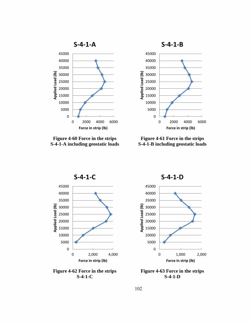
102
Figure 4-60 Force in the strips
S-4-1-A including geostatic loads
Figure 4-61 Force in the strips
S-4-1-B including geostatic loads
Figure 4-62 Force in the strips
S-4-1-C
Figure 4-63 Force in the strips
S-4-1-D
0
5000
10000
15000
20000
25000
30000
35000
40000
45000
0 2000 4000 6000
Ap
plie
d L
oad
(lb
)
Force in strip (lb)
S-4-1-A
0
5000
10000
15000
20000
25000
30000
35000
40000
45000
0 2000 4000 6000
Ap
plie
d L
oad
(lb
)
Force in strip (lb)
S-4-1-B
0
5000
10000
15000
20000
25000
30000
35000
40000
45000
0 2,000 4,000
Ap
plie
d L
oad
(lb
)
Force in strip (lb)
S-4-1-C
0
5000
10000
15000
20000
25000
30000
35000
40000
45000
0 1,000 2,000
Ap
plie
d L
oad
(lb
)
Force in strip (lb)
S-4-1-D
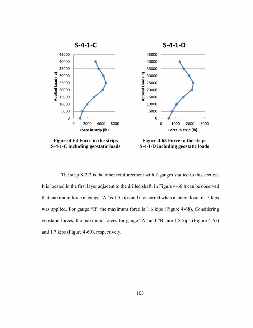
103
Figure 4-64 Force in the strips
S-4-1-C including geostatic loads
Figure 4-65 Force in the strips
S-4-1-D including geostatic loads
The strip S-2-2 is the other reinforcement with 2 gauges studied in this section.
It is located in the first layer adjacent to the drilled shaft. In Figure 4-66 it can be observed
that maximum force in gauge “A” is 1.5 kips and it occurred when a lateral load of 15 kips
was applied. For gauge “B” the maximum force is 1.6 kips (Figure 4-68). Considering
geostatic forces, the maximum forces for gauge “A” and “B” are 1.8 kips (Figure 4-67)
and 1.7 kips (Figure 4-69), respectively.
0
5000
10000
15000
20000
25000
30000
35000
40000
45000
0 2000 4000 6000
Ap
plie
d L
oad
(lb
)
Force in strip (lb)
S-4-1-C
0
5000
10000
15000
20000
25000
30000
35000
40000
45000
0 1000 2000 3000
Ap
plie
d L
oad
(lb
)
Force in strip (lb)
S-4-1-D

104
Figure 4-66 Force in the strips
S-2-2-A
Figure 4-67 Force in the strips
S-2-2-B
Figure 4-68 Force in the strips
S-2-2-A including geostatic loads
Figure 4-69 Force in the strips
S-2-2-B including geostatic loads
0
5000
10000
15000
20000
25000
30000
35000
40000
45000
0 1,000 2,000
Ap
plie
d L
oad
(lb
)
Force in strip (lb)
S-2-2-A
0
5000
10000
15000
20000
25000
30000
35000
40000
45000
0 1,000 2,000
Ap
plie
d L
oad
(lb
)
Force in strip (lb)
S-2-2-B
0
5000
10000
15000
20000
25000
30000
35000
40000
45000
0 1000 2000
Ap
plie
d L
oad
(lb
)
Force in strip (lb)
S-2-2-A
0
5000
10000
15000
20000
25000
30000
35000
40000
45000
0 1000 2000
Ap
plie
d L
oad
(lb
)
Force in strip (lb)
S-2-2-B

105
The force distribution near the drilled shaft is another interesting result obtained
from this test. In each layer, there is an instrumented strip at each side of the drilled shaft
(18 inches from the drilled shaft) and there is another instrumented strip at 77 inches from
the drilled shaft). The data from these gauges is used here to study the variation of forces
in direction parallel to the wall. In Figure 4-70 forces in first layer of strips are shown.
The “0” corresponds to the position of the drilled shaft. As it can be observed, the
distribution of forces around the drilled shaft is nearly symmetric. The distribution of
forces in the second layer near is not symmetric, especially at higher loads (Figure 4-71).
That could be because of asymmetric deformation of panels.
The results for the case with geostatic forces are shown in Figure 4-72 and Figure
4-73 for first and second layers of strips respectively. As expected a similar pattern is
observed.

106
Figure 4-70 Distribution of forces at each side of the drilled shaft in first layer of
strips. The “0” corresponds to the position of the drilled shaft
Figure 4-71 Distribution of forces at each side of the drilled shaft in second layer of
strips. The “0” corresponds to the position of the drilled shaft
-1,000
-500
0
500
1,000
1,500
2,000
-40 10 60 110
Forc
e(l
b)
Distance from the drilled shaft (inch)
Force in first layer of strips
L=5
L=10
L=15
L=20
L=25
L=30
L=35
L=40
0
500
1,000
1,500
2,000
2,500
3,000
3,500
4,000
4,500
-40 -20 0 20 40 60 80 100
Forc
e(l
b)
Distance from the drilled shaft (inch)
Force in Second layer of strips
L=5
L=10
L=15
L=20
L=25
L=30
L=35
L=40

107
Figure 4-72 Distribution of forces at each side of the drilled shaft in first layer of
strips including Geostatic loads. The “0” corresponds to the position of the drilled
shaft
Figure 4-73 Distribution of forces at each side of the drilled shaft in second layer of
strips including Geostatic loads. The “0” corresponds to the position of the drilled
shaft
-500
0
500
1,000
1,500
2,000
-40 -20 0 20 40 60 80 100
Forc
e(l
b)
Distance from the drilled shaft (inch)
Force in first layer of strips
L=5
L=10
L=15
L=20
L=25
L=30
L=35
L=40
0
500
1,000
1,500
2,000
2,500
3,000
3,500
4,000
4,500
5,000
-40 -20 0 20 40 60 80 100
Forc
e(l
b)
Distance from drilled shaft (inch)
Force in Second layer of strips
L=5
L=10
L=15
L=20
L=25
L=30
L=35
L=40

108
4.2.9.3. Pressure on the wall and drilled shaft
One pressure cell was installed on the drilled shaft and another one on the wall.
The results in terms of pressure on the drilled shaft against the lateral load are presented
in Figure 4-74. The maximum pressure on the drilled shaft was 17 psi. As it is seen in
Figure 4-75, the maximum pressure on the wall was 7.8 psi.
Figure 4-74 Pressure measured on the drilled shaft with the load cell
-5,000
0
5,000
10,000
15,000
20,000
25,000
30,000
35,000
40,000
45,000
-5 0 5 10 15 20
Forc
e(l
b)
Pressure (psi)
Drilled shaft
5
1
2
3
4
6
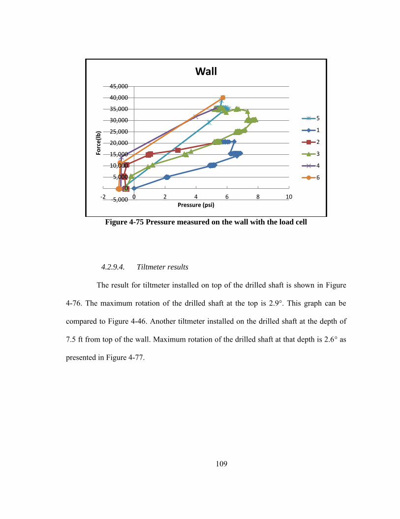
109
Figure 4-75 Pressure measured on the wall with the load cell
4.2.9.4. Tiltmeter results
The result for tiltmeter installed on top of the drilled shaft is shown in Figure
4-76. The maximum rotation of the drilled shaft at the top is 2.9°. This graph can be
compared to Figure 4-46. Another tiltmeter installed on the drilled shaft at the depth of
7.5 ft from top of the wall. Maximum rotation of the drilled shaft at that depth is 2.6° as
presented in Figure 4-77.
-5,000
0
5,000
10,000
15,000
20,000
25,000
30,000
35,000
40,000
45,000
-2 0 2 4 6 8 10
Forc
e(l
b)
Pressure (psi)
Wall
5
1
2
3
4
6

110
Figure 4-76 Tiltmeter result for the device installed on top of the drilled shaft
Figure 4-77 Tiltmeter result for the device installed on bottom of the drilled shaft
Figure 4-78 shows the rotation of top of the wall for different horizontal loads.
The maximum rotation on this graph is 2.2°. The result for the tiltmeter which was
0
10,000
20,000
30,000
40,000
50,000
0 0.5 1 1.5 2 2.5 3 3.5
Ap
plie
d L
oad
(lb
)
Rotation (degree)
Top of the drilled shaft
0
5,000
10,000
15,000
20,000
25,000
30,000
35,000
40,000
45,000
0 0.5 1 1.5 2 2.5 3
Ap
plie
d L
oad
(lb
)
Rotation (degree)
Bottom of the drilled Shaft

111
installed on the bottom of the wall is presented in Figure 4-79. As it can be seen in this
graph, rotation in this part of the wall is considerably smaller than the rotation of top of
the wall.
Figure 4-78 Tiltmeter result for the device installed on top of the wall
Figure 4-79 Tiltmeter result for the device installed on bottom of the wall
0
10,000
20,000
30,000
40,000
50,000
-0.1 0.4 0.9 1.4 1.9 2.4
Ap
plie
d L
oad
(lb
)
Rotation (degree)
Top of the wall
0
10,000
20,000
30,000
40,000
50,000
0 0.2 0.4 0.6 0.8 1 1.2
Ap
plie
d L
oad
(lb
)
Rotation (degree)
Bottom of the wall

112
4.2.9.5. Inclinometer results
After each step there was about 15 minutes for inserting the inclinometer probe
into the casing in the drilled shaft and the wall and read the results. Data collected by this
device was used to calculate drilled shaft and wall deformation toward the load direction
(A axis) and also the deformation perpendicular to the load direction (B axis).
The maximum deformation of top of the drilled shaft calculated in the step with
horizontal load of 40 kips is 5.4 inches (as presented in Figure 4-80). This deformation is
smaller than the 6.15 inches measured with the string pot. That is because the inclinometer
readings were performed after the unloading but the deformation from string pot was
measured when the load of 40 kips was applied. A plan view of showing the drilled shaft
deformation is presented in Figure 4-81. In this graph the origin (point: (0,0)) is the initial
position of the drilled shaft. It can be observed that it deforms toward the wall.
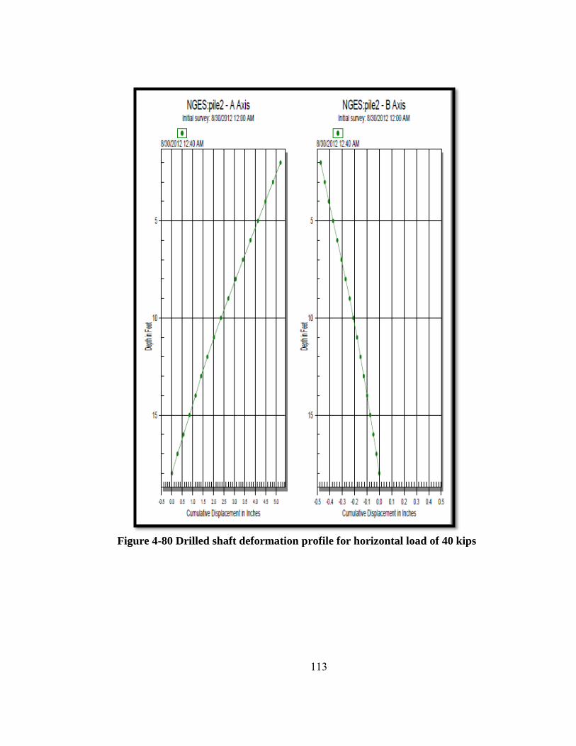
113
Figure 4-80 Drilled shaft deformation profile for horizontal load of 40 kips

114
Figure 4-81 Plan view of the drilled shaft deformation for horizontal load of 40 kips
The same procedure was applied for the wall. As it is shown in Figure 4-82, the
maximum deformation of the wall at the horizontal load of 40 kips is 2 inches. A plan
view showing the wall deformation is presented in Figure 4-83. The initial position of the
wall is at the point indicated as (0,0). It can be observed that the wall moved away from
the drilled shaft.

115
Figure 4-82 Wall deformation profile for horizontal load of 40 kips

116
Figure 4-83 Plan view of the wall deformation for horizontal load of 40 kips
The maximum deformation of the drilled shaft at the horizontal load of 35 kips
is 4 inches (see Figure 4-84). The maximum drilled shaft deformation in this step measured
with the string pot is 4.03 inches. A plan view of the drilled shaft deformation for this step
is presented in Figure 4-85. This procedure was applied for all the loading steps.
The wall deformation profile for the step corresponding to 35 kips of horizontal
load is shown in Figure 4-86. The plan view of wall deformation for this step is presented
in Figure 4-87.

117
Figure 4-84 Drilled shaft deformation profile for horizontal load of 35 kips

118
Figure 4-85 Plan view of the drilled shaft deformation for horizontal load of 35 kips

119
Figure 4-86 Wall deformation profile for horizontal load of 35 kips
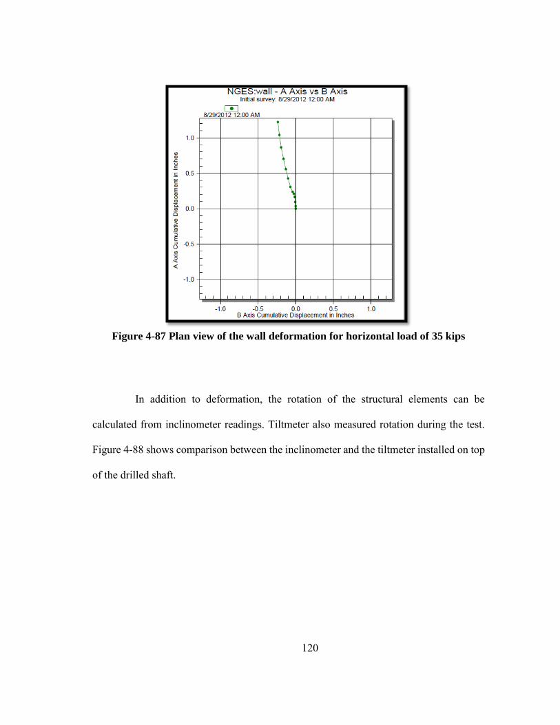
120
Figure 4-87 Plan view of the wall deformation for horizontal load of 35 kips
In addition to deformation, the rotation of the structural elements can be
calculated from inclinometer readings. Tiltmeter also measured rotation during the test.
Figure 4-88 shows comparison between the inclinometer and the tiltmeter installed on top
of the drilled shaft.

121
Figure 4-88 Comparison between tiltmeter and inclinometer for top of the drilled
shaft
The comparison between the inclinometer and the tiltmeter installed on bottom
of the drilled shaft is shown in Figure 4-89.
Figure 4-89 Comparison between tiltmeter and inclinometer for bottom of the
drilled shaft
0
0.5
1
1.5
2
2.5
3
0 1 2 3
Ro
tati
on
cal
cula
ted
fro
m t
iltm
ete
r (d
egr
ee
)
Rotation calculated from inclinometer (degree)
0
0.5
1
1.5
2
2.5
3
0 1 2 3
Ro
tati
on
cal
cula
ted
fro
m t
iltm
ete
r (d
egr
ee
)
Rotation calculated from inclinometer (degree)

122
In real sites (i.e. projects selected by TxDOT) the inclinometer cannot be used
in the drilled shaft because of the bridge deck. To get the drilled shaft deformation more
tiltmeters are installed on these projects. As it can be seen in Figure 4-88 and Figure 4-89
the results from tiltmeters match quite well the results from the inclinometer, especially
when comparing small deformation.
4.2.9.6. Results from LIDAR
A LIDAR (or LiDAR: Light Detection and Ranging) was used to achieve a
better understanding of the wall and the drilled shaft deformations. The LiDAR scanned
the wall surface after each step. The scan related to the initial condition (i.e. before
applying the load) is presented in Figure 4-90.
The LIDAR plan view of the column at the end of the test is shown in Figure
4-91. The deformation of top of the drilled shaft and top of the wall can be calculated by
comparing these two pictures. The final deformation of top of the drilled shaft according
to LIDAR is 4.7 inches and the final deformation of top of the wall is 2.7inches that
matches the results from string pot (4.94 inches for top of the drilled shaft and 2.88 inches
for top of the wall).

123
Figure 4-90 LIDAR plan views of the drilled shaft and the wall for initial condition
Figure 4-91 LIDAR plan views of the drilled shaft and the wall at the end of the test

124
4.2.9.7. Wall Deformation
Photogrammetry was used in this research to obtain the deformation contours of
the face of the wall at different loading steps. The deformation in the following plots is
presented in millimeter. The zero point in horizontal axis is where the drilled shaft was
installed. Figure 4-92 shows the deformation contour for horizontal load of 5 kips. The
maximum deformation in this step is 0.5 mm. The maximum deformation for the step with
horizontal load of 10 kips is 2.5 mm (see Figure 4-93). As it is shown in Figure 4-94, the
bigger part of wall deformed at horizontal load of 15 kips. The corresponding maximum
deformation is 7.6mm. The deformation contour for a horizontal load of 20 kips is
presented in Figure 4-95. The maximum deformation in this step is 13 mm. In the
subsequent steps, the deformations concentrated on the top panel in front of the drilled
shaft, while the deformation of other panels was very small. As shown in Figure 4-96, for
the step corresponding to 25 kips the deformation for other panels are considerable. The
maximum deformation in this step is 19.5 mm. For the horizontal load of 30 kips, the
maximum deformation of the wall is 27 mm (see Figure 4-97). Figure 4-98 shows the
contour of deformation for horizontal deformation of 35 kips. The maximum deformation
in this step is 50.1mm. The horizontal load in the last step was 40kips. The associated
deformation contour for this step is presented in Figure 4-99. The maximum deformation
in this case is 101.1 mm.
The maximum deformations in all of steps occur at top of the wall in front of the
drilled shaft. These results confirmed the maximum deformation measured by string pot.

125
Figure 4-92 Wall deformation contour for horizontal load of 5 kips
Figure 4-93 Wall deformation contour for horizontal load of 10 kips
12
38.7
86.7
134.6
182.6-292 -146 -72 13 73 132
De
pth
(cm
)
Distance from the shaft (cm)
Wall deformation (mm) for 5kips
0.4-0.5
0.3-0.4
0.2-0.3
0.1-0.2
0-0.1
12
38.7
86.7
134.6
182.6
-292 -146 -72 13 73 132
De
pth
(cm
)
Distance from the shaft (cm)
Wall deformation (mm) for 10kips
2-2.5
1.5-2
1-1.5
0.5-1
0-0.5

126
Figure 4-94 Wall deformation contour for horizontal load of 15 kips
Figure 4-95 Wall deformation contour for horizontal load of 20 kips
12
38.7
86.7
134.6
182.6
-292 -146 -72 13 73 132
De
pth
(cm
)
Distance from the shaft (cm)
Wall deformation (mm) 15kips
6-8
4-6
2-4
0-2
12
38.7
86.7
134.6
182.6
-292 -146 -72 13 73 132
De
pth
(cm
)
Distance from the shaft (cm)
Wall deformation (mm) 20kips
12-15
9-12
6-9
3-6
0-3
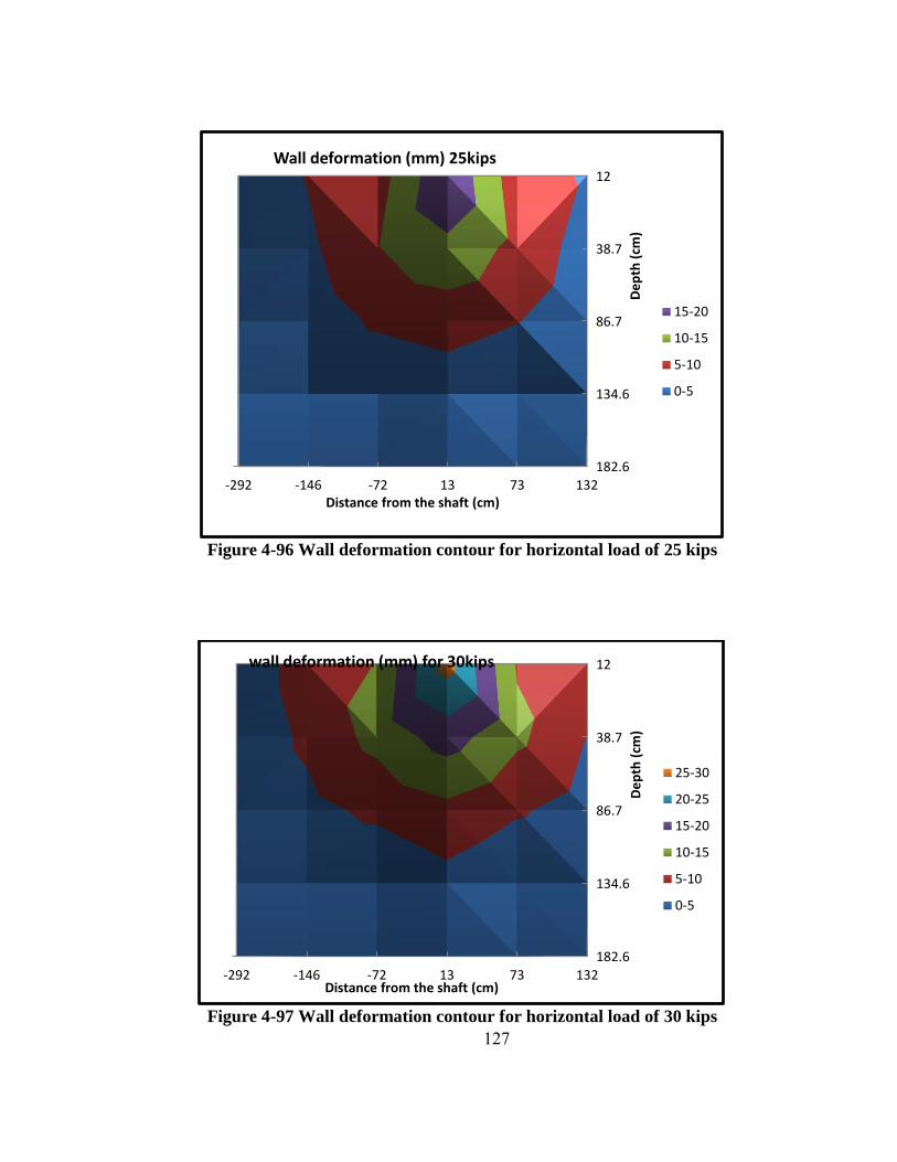
127
Figure 4-96 Wall deformation contour for horizontal load of 25 kips
Figure 4-97 Wall deformation contour for horizontal load of 30 kips
12
38.7
86.7
134.6
182.6
-292 -146 -72 13 73 132
De
pth
(cm
)
Distance from the shaft (cm)
Wall deformation (mm) 25kips
15-20
10-15
5-10
0-5
12
38.7
86.7
134.6
182.6
-292 -146 -72 13 73 132
De
pth
(cm
)
Distance from the shaft (cm)
wall deformation (mm) for 30kips
25-30
20-25
15-20
10-15
5-10
0-5

128
Figure 4-98 Wall deformation contour for horizontal load of 35 kips
Figure 4-99 Wall deformation contour for horizontal load of 40 kips
12
38.7
86.7
134.6
182.6
-292 -146 -72 13 73 132
De
pth
(cm
)
Distance from the shaft (cm)
Wall deformation (mm) 35kips
50-60
40-50
30-40
20-30
10-20
0-10
12
38.7
86.7
134.6
182.6
-292 -146 -72 13 73 132
De
pth
(cm
)
Distance from the shaft (cm)
Wall deformation (mm) 40kips
100-120
80-100
60-80
40-60
20-40
0-20

129
Other devices and methods used in this test to measure wall deformation such
as inclinometer and Lidar.
4.2.10. Discussion
Fortunately all of the instruments and devices in this test worked properly and
very valuable data were collected. These data is very useful for calibrating the numerical
models. One the numerical models are calibrated they can be used to explore the behavior
of the wall-shat system under different loading conditions, geometries and boundary
conditions.
An interesting result obtained in this study is related to the distribution of forces
in the strips. It has been observed that the highest force in the strip did not occur at the
maximum horizontal load. As it can be seen in Figure 4-58, the maximum force in the
strip happened when a horizontal load of 25 kips was acting on the drilled shaft. Another
relevant result is that force in the second layer of strips is greater than the force in the top
layer.
4.3. Monitoring at TxDOT site at Bastrop
4.3.1. Real project introduction
The project is an overpass in SH 71 over FM 20 conjunction as shown in Figure
4-100. The overpass is from west of FM 20 to east of FM 969 and the length is 1.354
miles. The project started in September 2012.

130
Figure 4-100 Location for project in Bastrop
As it is shown in Figure 4-101 there are two Mechanically Stabilized Earth
(MSE) wall in this overpass, i.e. the east wall and west wall. Based on the construction
schedule, east wall was chosen for this research.
Height of the east wall is 15 ft and its length is 109 ft. The backfill material is
crushed rock and the reinforcement used in this wall is metal grids. The length of the grids
varied with the vertical position. For the 2 top rows of grids the length is 18 ft. The detail
of the east wall is shown in Figure 4-102.

131
Figure 4-101 Plan view of the overpass
Figure 4-102 East wall detail

132
4.3.1.1. Instrumentation
The adopted instrumentation for this project site is similar to the one adopted for
the full scale test at NGES. A (slight) difference is that in the full scale test most of the
devices (i.e. inclinometer casing, tiltmeters) were installed outside of the wall but in this
project they were installed in (the internal) face of the wall. This difference is because this
wall is related to an actual bridge and the taskmaster did not want any exposed device on
the wall. The instruments (i.e. gauges, tiltmeters) were installed during construction in
different layers.
Inclinometer:
In this project the inclinometer is not used for measuring the deflections of the
drilled shaft, because there is bridge deck on top of the drilled shaft and there is no room
to handle the inclinometer probe in the casing. Three tiltmeters were installed on the drilled
shaft and other three tiltmeters were installed on the wall. This was done to have a better
understanding of the wall and shaft deformations.

133
Figure 4-103 Drilling the hole for the inclinometer casing
Figure 4-104 Extended casing attached to the wall

134
Figure 4-105 Casing at top of the wall
Tiltmeter
As mentioned before, in the actual projects 3 tiltmeters were installed on the
drilled shaft and another 3 were installed on the wall. One tiltmeter was installed at the
bottom, one at the middle and one at top of the wall. Tiltmeters on the drilled shaft were
installed at the same positions adopted for the ones on the wall. To protect the tiltmeters
from compaction and other external actions, metal boxes were used (Figure 4-106). PVC
tubes were used to protect wires (Figure 4-107).

135
Figure 4-106 Tiltmeters installed on the wall
Figure 4-107 PVC tubes used for protecting wires

136
Strain gauge
A total of 8 full bridge circuits were used in this project, 4 per each layer (Figure
4-108). In order to install the strain gauges on the grids, first it was attempted to install
gauges directly on the bars, as shown in Figure 4-109. Then, looking at the results of a
loading test performed on the bar, it was concluded that this solution was not acceptable.
Another option was to cut the bar in target positions, weld a metal strip with the same
section area as the bar, and install the strain gauges on that strip (Figure 4-110). This option
was finally selected.
Figure 4-108 First and second layers of grids

137
Figure 4-109 Strain gauge installed on the bar
Figure 4-110 Strips attached to the bars
To protect gauges against moisture and rupture, PVC tape were rapped around
them and in the field, before putting the crushed rock on top of them. Also a sand bag
was placed on top and beneath of each gauges to prevent that the crushed rock touching
the gauges (Figure 4-111)

138
Figure 4-111 Sand bags for protecting the gauges
Pressure cell
A pressure cell was used in this wall. It was installed at the middle of the top
panel. It is the same as the one used in the full scale test. To gather good results from the
pressure cell, it is recommendable that a uniform pressure act on it. In crushed rock this is
difficult, because this material tend to apply the load to the cell pressure in a manner that
is more similar to point loads, rather than uniform pressure, and this may lead to imprecise
measurements. To solve this problem, a sand bag was installed in front of the cell to assist
to an uniform distribution of pressure (Figure 4-112).

139
Figure 4-112 Sand bag used on pressure cell to uniform the pressure
Data Acquisition System
CR1000 is the data logger used in this project site. It is the same adopted as data
logger to collect data from tiltmeters in the full-scale test at Riverside Campus. To provide
power for the data logger, a solar panel was installed on the site and a battery was used to
accumulate power. A Data Acquisition Box installed on the top of the wall (as shown in
Figure 4-113(a)) and the solar panel installed on top of the riprap to be exposed to sunshine
(as shown in Figure 4-113(b))

140
(a) (b)
Figure 4-113 Data Acquisition installed at Bastrop site a) Box b) Solar panel
4.3.1.2. Results
Data from this site is being collected since 27th of December 2013. The
corresponding data for the last four months is presented in this Chapter.
Strain gauge results
A total of eight strain gauges were used in this project site. Four of them were
installed on the top layer of metal grids which are labeled with “T” and four of them
installed on the second layer of metal grids from the top which are labeled with “B”. The
adopted notation for the strain gauges is shown in Figure 4-114. The sets of data gathered
for all of the strain gauges are presented in Figure 4-115.

141
Figure 4-114 Strain gauge numbering
Figure 4-115 Strain gauge data from Bastrop site
As it is shown in Figure 4-115, no changes in the forces in the strips were
observed in this period of time.
0
200
400
600
800
1000
1200
1400
27-Dec 21-Jan 15-Feb 12-Mar 6-Apr
Forc
e in
the
strip
(lb)
Date
TL1
TR1
TL2
TR2
BL1
BR1
BL2
BR2

142
Pressure cell
As it was mentioned before, in this project site we use one pressure cell on the
wall at a depth of 9 inches from top of the wall. The data from the pressure cell is presented
in Figure 4-116. Also I this case no changes are observed during the analyzed period of
time.
Figure 4-116 Pressure cell data for Bastrop site
Tiltmeter
A total of six tiltmeters were installed in this project site. Thye were coded as
follows: “TW” on top of the wall, “MW” on middle of the wall, “BW” on bottom of the
wall, “TS” on top of the drilled shaft, “MS” on middle of the drilled shaft and “BS” on
bottom of the drilled shaft. The data gathered for these tiltmeters are shown in Figure
4-117.
0
0.5
1
1.5
2
27-Dec 21-Jan 15-Feb 12-Mar 6-Apr
Pres
sure
on
the
wal
l (ps
i)
Date

143
Figure 4-117 Tiltmeter data from Bastrop site
As it is shown in this figure, there have no changes in their initial angles.
Inclinometer
The results after four months are presented in Figure-4-118. The “A” axis is the
axis perpendicular to the wall and “B” axis is the one parallel to the wall. Also in this case,
no changes in the wall deflection were detected with the inclinometer.
0
0.5
1
1.5
2
2.5
3
27-Dec 21-Jan 15-Feb 12-Mar 6-Apr
Ang
le (d
egre
e)
Date
TW
MW
BW
TS
MS
BS

144
(a) (b)
Figure-4-118 Inclinometer results for Bastrop site a) toward the wall b) parallel
with the wall
4.4. Conclusion
The full-scale test was performed successfully at Riverside Campus at Texas
A&M University. All of the devices worked perfectly during the test and valuable data
was gathered from this test. The test took about 4 hours to perform and 19 people were
involved in the test with the PhD candidate lead.
The real project site in Bastrop, Texas was monitored for six months. All of the
devices installed on the wall and drilled shaft during the construction and collecting data
started when the bridge opened to traffic. The initial plan was to monitor this project site
for 16 months but due to contractor delay, the monitor period reduced to six months.
The real project site in Salado, Texas was instrumented and ready for collecting
data but because of construction delay no data was gathered from this site.
05
10152025303540
-1 -0.5 0 0.5 1
casi
ng h
eigh
t (ft)
Displaecement (in)
A- Axis
0
10
20
30
40
-1 -0.5 0 0.5 1
casi
ng h
eigh
t (ft)
Displaecement (in)
B- Axis

145
5. NUMERICAL MODELING
5.1. Introduction
This chapter presents the numerical modeling of a drilled shaft built within an
MSE wall. This chapter covers model calibration, parametric study, numerical results and
discussions. The model calibration (section 5.2) is based on the pullout test data and the
field test information. The pullout test data were performed in the framework of the
TxDOT Project 0-6493 (at Texas Tech University), while the field test data was gathered
from the test completed at the Riverside Campus of Texas A&M University in August
2012, in the context of the research related to this Thesis. Once the numerical model was
calibrated, it was used to investigate the influence of various factors on the performance
of the drilled shaft and the MSE wall. This part was covered in section 5.3 and 5.4. The
numerical software FLAC3D (version 4.0) was adopted for this study.
5.2. Simulation of the pullout test with cable elements
According to FLAC 3D version 4 manual (Itasca, 2006), the cable elements are
used to model the strips. Two types of springs are contemplated in FLAC 3D software,
shear and normal springs. Normal springs are mainly used for beam elements, while shear
springs are used for cable elements. As the shear spring deforms, the shear force, Fs, per
unit length in the spring increases. Deforming the spring implies that the distance between
the node of the structural component and the hosting media changes. For a given
deformation, the spring shear force increases with increasing spring stiffness (ks) and it
reaches a limiting value of Fsmax / L (as shown in Figure 5-1a).

146
The parameters to be use in the model for shear spring are Фs and Cs. Pullout
tests were conducted on metal strips by Texas Tech University (Lawson et al., 2013). The
tests were performed at three different depths (i.e. different confining pressure) as shown
in Figure 5-2.
|us |
| Fsmax|
L
| Fs|
L
σmp
φs
| Fsmax|
L
Cs
Ks
1
(a) (b)
Figure 5-1 Shear spring modulus (Itasca, 2006)
Fsmax is the pullout force for the deformation of 0.75 inch. These tests were
performed at 3 different depths and for each test a point was obtained in the plain Fsmax /
L versus σmp (presented in Figure 5-3). The best fitting line was drawn through these 3
points. According to the FLAC 3D user’s guide (Itasca, 2006), the slope of this line is Фs
and the intercept of the line with the Fsmax / L axis is the Cs as shown in Figure 5-1. (P is
the perimeter of the strip). The shear friction angle (Фs) is 57.6ᵒ and the shear cohesion
(Cs) is 2.64 psi. Note that these parameters are called shear friction angle and shear
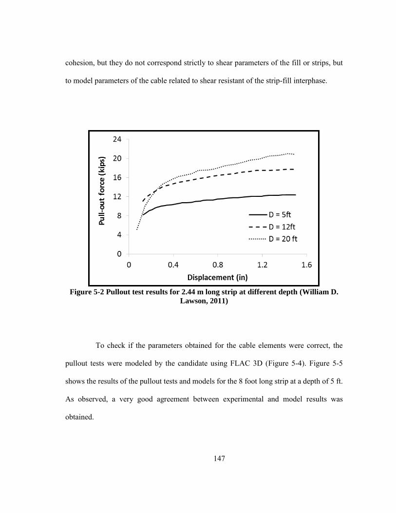
147
cohesion, but they do not correspond strictly to shear parameters of the fill or strips, but
to model parameters of the cable related to shear resistant of the strip-fill interphase.
Figure 5-2 Pullout test results for 2.44 m long strip at different depth (William D.
Lawson, 2011)
To check if the parameters obtained for the cable elements were correct, the
pullout tests were modeled by the candidate using FLAC 3D (Figure 5-4). Figure 5-5
shows the results of the pullout tests and models for the 8 foot long strip at a depth of 5 ft.
As observed, a very good agreement between experimental and model results was
obtained.

148
Figure 5-3 Calibration of shear spring for metal strips
Figure 5-4 FLAC 3D model of pullout test for 8ft strip in depth of 5 ft

149
Figure 5-5 Results for test and modeling of pullout for 8ft strip in depth of 5 ft
5.3. Modeling the pull-out tests discretizing the strip in the mesh
The interesting point about the use of metal strips as reinforcement for MSE
walls is their high friction factor. The friction factor (F*) is defined as:
*
'2
p u ll o u t
v a
TF
b L
(5.1)
where Tpull-out is the pull-out force in the strip for 0.75 in of displacement, α is
the scale factor which is equal to 1 for metal strips, σ’v is the vertical effective stress, b is
the width of the strip, and La is the length of the strip. For a smooth strip without the
bumps, F* is tentatively equal to tan(φ) which is about 0.6 but for the actual strip with
bumps it can be much more higher (about 6.15). Figure 5-6 present the recommended
friction factor values by (American Association of State Highway & Transportation

150
Officials. Subcommittee on Bridges, 2010), the friction factor from the pullout test and
the numerical model for a 2.44 m strip at different depths.
Figure 5-6 Pullout resistance factor vs. depth
To study in more detail the friction factor and to check ift this high friction factor
are justifiable, an actual foot long strip was modeled in FLAC 3D. The details related to
the modeling of the strip are shown in Figure 5-7 and the full model is presented in Figure
5-8.
The results of the pull-out modeling of the actual strip are plotted in Figure 5-10.
The results from the pull-out tests are also plotted in the same graph. The important
parameter in this modeling is the number of bumps per foot of the strip. The arrangement
0
5
10
15
20
25
30
35
40
45
0 1 2 3 4 5 6 7 8
Dep
th o
f fill
(ft)
Pullout resistance factor(F*)
F* from the test
F* from the model
TxDOT 0-6493 Data
AASHTO (2010) F* forribbed strips

151
of the bumps on the strip is not important. Another modeled prepared for evenly
distributed bumps on the strips and the results were the same as the actual strip.
Figure 5-7 Detail of modeled strip (actual strip)
Figure 5-8 Completed model of actual strip
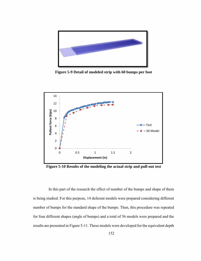
152
Figure 5-9 Detail of modeled strip with 60 bumps per foot
Figure 5-10 Results of the modeling the actual strip and pull-out test
In this part of the research the effect of number of the bumps and shape of them
is being studied. For this purpose, 14 deferent models were prepared considering different
number of bumps for the standard shape of the bumps. Then, this procedure was repeated
for four different shapes (angle of bumps) and a total of 56 models were prepared and the
results are presented in Figure 5-11. These models were developed for the equivalent depth
0
2
4
6
8
10
12
14
0 0.5 1 1.5 2
Pu
llou
t fo
rce
(ki
ps)
Displacement (in)
Test
3D Model

153
of 5 feet. For this depth the steel failed developing a friction factor of 12.5 and higher. In
order to capture the whole behavior in a unique graph, the strength of the steel was
increased in the model to a higher (fictitious) value than the actual steel strength. In this
way, the steel does not fail and it is possible to study the effect of bumps on the pull out
capacity of the strip.
Figure 5-11 Friction factor for different cases
5.4. Simulation of the Load Test at Riverside Campus
The reinforced soil, retained soil, and foundation soil were modeled as linearly
elastic-perfectly plastic materials, with Mohr-Coulomb failure criterion (i.e. the so-called
Mohr-Coulomb model). The Mohr-Coulomb model has been successfully used in other
studies to simulate MSE walls (Hatami & Bathurst, 2005; B. Huang, Bathurst, & Hatami,
0
5
10
15
20
25
0 10 20 30 40 50 60
F.S
Number of ribs per one foot
alpha=35
alpha=45
alpha=55
alpha=65

154
2009; J. Huang et al., 2011). Those studies showed that the Mohr-Coulomb model could
reproduce satisfactorily the experimental observations. Based on this background
information, the Mohr-Coulomb model was adopted in this study.
The reinforcement was modeled as a structural element (i.e. by using the cable
element already implemented in FLAC3D). The cable element behaves elastically upon
reaching tensile or compressive strength. The interaction between reinforcement and
backfill soil was simulated by Mohr-Coulomb sliders, which are linearly-elastic perfectly-
plastic springs formulated using the Mohr-Coulomb failure criteria.
The MSE wall facing panel was simulated as a linear elastic material. The
contacts between the panels were also modeled by means of Mohr-Coulomb sliders.
Considering the interlocking existing between the panels, the cohesion at the interface face
was assumed to be equal to the shear strength of the concrete. The connection between
the panel and the reinforcement was assumed rigid (i.e. no connection failure was allowed
during the numerical modeling). The drilled shaft was simulated as an elastic material
and typical values for concrete were adopted for the Young modulus and Poisson’s ratio
(Table 5-1).
The modeling of the wall was carried in steps. The initial stress field of the
foundation soil was first established and then construction of the MSE wall was simulated
by lifts mimicking the actual construction process. A concentrated lateral force was
applied at the top of the drilled shaft and this load was increased gradually with equal
increments. The numerical model was calibrated using the data obtained from the field
test at Riverside Campus of Texas A&M University.

155
5.4.1. Natural soil
The natural soils affect the behavior of the wall and the drilled shaft. At the
location of the tests at the riverside campus the natural soil is composed of a thin layer of
black clay (about 30 cm) overlying a thick layer of clean sand. The undrained shear
strength of the black clay measured by pocket penetrometer is 3394psi. The sand in the
lower layer is a poorly graded sand (classified according to the USCS as SP) with a
coefficient of uniformity (Cu) equals to 3.5 and a coefficient of curvature (Cc) equals to
0.88. To obtain the strength parameters of the clean sand layer pressuremeter tests (PMT)
were used. Three pressuremeter tests were performed at different depths. Parameters
obtained from the PMT were used to check the bearing capacity of the natural soil. These
parameters were also used in the numerical modeling of the test. The results of the PMT
for depths of 2.0 ft, 4.4ft and 6.9 ft are presented in Figure 5-12. The vertical axis
corresponds to the water pressure in the probe (P) and the horizontal axis is the ratio of
change in probe radius to the initial radius. The slope of this graph in the elastic region
equals to 2G (i.e. twice the shear modulus, (Briaud, 1992). The modulus of elasticity
obtained from the PMT for natural sand was 1563.5 psi.

156
Figure 5-12 Natural soil PMT result at different depth
The natural soil was modeled as a single layer material and the Mohr-Coulomb
constitutive model was adopted in the simulations. Based on existing information related
to the site no cohesion was considered and a friction angle of 30ᵒ was assumed. The PMT
results were used to calculate bulk and shear modulus according to (Briaud, 1992).
5.4.2. Backfill soil
The backfill material used in this investigation was a fine to medium sand. This
sand satisfies the requirements for a backfill for MSE wall specified in AASHTO LRFD
Bridge Construction Specifications, FHWA Publication No. FHWA-10-024 and TxDOT
Specification Item No 423/Type B select backfill (American Association of State Highway
& Transportation Officials. Subcommittee on Bridges, 2010; Elias, Barry, & Christopher,
1997). The coefficient of uniformity (Cu) for this soil is 4.5 and the coefficient of curvature
(Cc) is 0.8. Therefore, according to the USCS the soil is classified as a poorly graded sand

157
(SP). The average dry density and water content are 111.4 pcf and 3%, respectively. These
values were determined by means of the nuclear density probe (ASTM D6938-10). This
dry density represents 95% of the maximum dry density obtained in the modified Proctor
test for the backfill material (ASTM D1557-12, 2012).
To determine the backfill sand parameters two types of tests were performed:
laboratory tests (triaxial), and in-situ tests (PMT). These parameters were used to check
the wall stability and also in the numerical modeling of the wall. Triaxial tests were
performed at 3 different confining pressures, which are associated with the different
depths of the strips instrumented in this research. The dry density obtained from the
nuclear density tests was adopted to prepare the soil sample in the lab. In the triaxial tests
it was observed that the sand behaves like a loose sand. The result of the triaxial tests for
backfill material is presented in Figure 5-13. The friction angle for this material is around
27.3° (i.e. =27.3°) and the cohesion around 0.79 psi (i.e. c=0.79 psi). Pressuremeter tests
were also performed at different depths (according to the depth of strip layer). The results
of PMTs for different depths are shown in Figure 5-14, where the variation of these values
with depth can be observed.
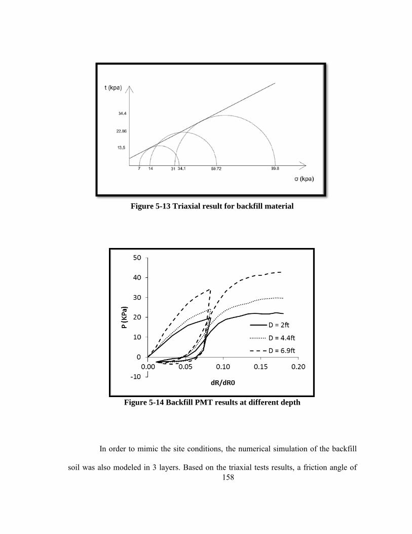
158
Figure 5-13 Triaxial result for backfill material
Figure 5-14 Backfill PMT results at different depth
In order to mimic the site conditions, the numerical simulation of the backfill
soil was also modeled in 3 layers. Based on the triaxial tests results, a friction angle of

159
27.3° and cohesion of c=0.79 psi were assumed. The bulk and shear moduli were estimated
from the PMT tests for different layers according to Briaud (2005).
5.4.3. Drilled shaft
There were two options to model the drilled shaft. One of them was to model
the pile as a structural element; which did not need to be included in the discretization (i.e.
as a part of the mesh), but interface elements between the shaft and the soil are required.
The other option was to model the actual shaft as an additional component of the system,
with the corresponding mesh and then assign properties of the concrete to these elements.
In this research the second option was adopted and the shaft was modeled as an actual
shaft with elastic properties.
5.4.4. Wall panels
The wall panels were modeled as actual panels, and concrete properties were
assigned to them. The actual wall is not uniform and there are gaps between panels. The
panels are connected together by means of shear keys. There are two options to simulate
the panels. One of them is to model actual gaps between panels and shear keys. (Hatami
& Bathurst, 2005) concluded that the modeling of the actual panels and the interlocking
between them would not improve significantly the numerical results. They also performed
some tests on modular blocks and came to a conclusion that a friction angle of 57ᵒ and
apparent cohesion of 6.67 psi were good parameters to model the strength behavior of the
MSE wall panels. They mentioned that under this condition, shear failure between the
blocks would not happen. The other option is to model the wall as an uniform material,
but with reduced strength parameters in comparison to concrete. (Yoo & Kim, 2008)

160
successfully used reduced modulus in their research. They used elastic modulus of 300
MPa for the wall. (J. Huang et al., 2011) also used the same parameters in their research.
In this research, a reduced modulus of 300 MPa was used for the panels.
5.4.5. MSE wall model
Once all the necessary parameters to model the MSE wall were defined, the 3D
model for the MSE wall was prepared. Table 5-1 presents all the model parameters
adopted to simulate the full-scale test, including: soil parameters (for both natural soil and
backfill material, estimated from PMT and triaxial tests), parameters for the drilled shaft;
panels parameters (adopted based on the manufacturers specifications), and the parameters
for metal strips calculated from the pullout test from Texas Tech.
The parameters mentioned above were used to create the 3D model of the MSE
wall in FLAC 3D program. A total of 22000 elements were used to model the wall and 5
materials were used to represent the different components of the physical model presented
in Figure 5-16.

161
Table 5-1 Properties used in the program
Material Constitutive Model Properties
Natural soil Mohr-Coulomb Ф’=30ᵒ , C’=0 , ϒ= 114.6 pcf B=1610 psi, G= 536.6 psi
Backfill soil first layer Mohr-Coulomb Ф’=27.3ᵒ , C’=0.79 psi , ϒ= 114.6 pcf
B=680 psi, G= 226.26 psi
Backfill soil second layer Mohr-Coulomb
Ф’=27.3ᵒ , C’=0.79 psi Kpa , ϒ= 114.6 pcf
B=475.7 psi, G= 158 psi Mpa Backfill soil third
layer Mohr-Coulomb Ф’=27.3ᵒ , C’=0.79 psi , ϒ= 114.6 pcf B=455.4 psi, G= 152.3 psi
Drilled shaft Elastic (isotropic) B=3.6e6 psi , G=1.2e6 psi ϒ= 159 pcf
MSE wall facing Elastic (isotropic) B=3.6e4 psi , G=1.7e4 psi ϒ= 159 pcf
Metal Strip Elastic-perfectly plastic
E=3.04e7 psi , Ks=942 psi, Фs=57.6 , Cs=2.64 psi
5.4.6. Loading protocol
The loading test was performed statically and under controlled load conditions.
The horizontal load was applied by means of a hydraulic jack by pulling the shaft against
the wall. The load was applied by steps of 5 kips (22.24 KN). Each step lasted around 15
minutes to have enough time for collecting data. Two unloading stages were performed.
The first one was at the load of 20 kips (88.96 KN) and the second unloading was at the
load of 35 kips (155.69 KN). The failure occurred at the horizontal load of 40 kips (177.93
KN). The horizontal load versus time is plotted Figure 5-15. The loading protocol was
fully discussed in Chapter 4.

162
Figure 5-15 Loading steps
The same loading protocol was adopted in the numerical modeling. The
horizontal movements of the wall and the shaft after applying 25 kips and 40 kips load are
presented in Figure 5-17 and Figure 5-18.
0
5
10
15
20
25
30
35
40
45
0 50 100 150 200
Load
(ki
ps)
Time (min)

163
Figure 5-16 Different parts of the MSE wall Model

164
Figure 5-17 Deformation of the wall after applying 25 kips of horizontal load

165
Figure 5-18 Deformation of the wall after applying 40 kips of horizontal load
Deformation of the drilled shaft and the MSE wall from the numerical models
are presented in Figure 5-19.
(a) (b)
Figure 5-19 Deformation of the drilled shaft and the MSE wall (a) side view (b) top
view

166
Deformations of top of the shaft for both test and model are drawn in Figure
5-20. It can be seen that he model capture quite well the behavior observed in this test.
Figure 5-20 Deformation of top of the shaft for the test and model
The results for the deformation at the top of the MSE wall, for both the test and
the model, are presented in Figure 5-21. As it was discussed before, to model the interlocks
between the panels in the facing of the wall, a reduced modulus for the panels was adopted.
This can be one of the reasons for the slight differences observed at the beginning of the
tests between experimental and modeling results.

167
Figure 5-21 Deformation of top of the wall for the test and model
The cable elements (i.e. a type of element available in FLAC-3D) were used to
simulate the metal strips. The arrangement of strips in the model and the force in the strips
when a horizontal load of 25 kip was applied is presented in Figure 5-22. It can be seen
that the force in the strips at second layer is greater than the top layer. This feature of
behavior was also observed in the full scale test.

168
Figure 5-22 Forces in the strips after horizontal load of 25 kips
A comparison between tests and model results for the force developed in the
strip located in the second layer in a position near the drilled shaft is shown in Figure 5-23.
Also in this case, a quite good matching between experiments and modeling are observed.

169
(a) (b)
Figure 5-23 Force in the strip “S-4-1-B” according to (a) horizontal load on the
shaft (b) wall displacement
As mentioned before, all of the parameters used in numerical modeling were
obtained from independent laboratory or in-situ tests. The reference values related to metal
strips were obtained from the pull out tests performed at Texas-Tech (Lawson et al., 2013).
To expalore the sensitivity of the model results respect to the model parameters associted
with the cable element 3 different Фs for the strips were considered in the numerical
analyses. The one obtained from the pull out test, i.e. Фs=57.6ᵒ, another higher value
Фs=70ᵒ and a reduced one Фs = 45ᵒ. The results showing the response of the strip for these
three values is presented in Figure 5-24.

170
Figure 5-24 Forces in the strip for different Фs
It can be seen that with the higher value of the friction angle for the strips, better
results were obtained. However, this higher Фs affected negatively other results of the
model, such as wall deformation and drilled shaft deformation.
As it can be seen in Figure 5-23 there is a peak in the graph. The soil between
the drilled shaft and the MSE wall failed after a 25 kips of horizontal load on the drilled
shaft. The soil is in the plastic zone and that is the reason for the peak in that graph. The
plastic zone for different applied horizontal loads on top of the drilled shaft is presented
in Figure 5-25.

171
30kips
35kips
40kips
30kips
35kips
40kips
Figure 5-25 Plastic zone for different values of horizontal load on top of the drilled
shaft
A numerical model was prepared for a case without the MSE wall (Figure 5-26).
The aim of this analysis was to study the effect of the MSE wall on the horizontal capacity
of the drilled shaft

172
Figure 5-26 Geometry of the case without the wall
As it can be seen in Figure 5-27, for a deformation at the top of the shaft equal
to 6 inches (which was the maximum deformation observed in the full scaled test), the
maximum horizontal load predicted by the model for the case with the wall is 40 kips;
while for the case without the wall is 10.84. This implies that the horizontal load is 75%
lower in the case without the wall.

173
Figure 5-27 Comparison between the case with the wall and the case without the
wall
5.5. Parametric study
5.5.1. Outline of the parametric study
The parametric study investigates the influence of various factors on the
performance of the laterally loaded drilled shaft built within an MSE wall. One case was
selected as the baseline case, for subsequent cases one parameter per time was varied
respect to the baseline case to investigate the influence of one particular factor on the
performance of the drilled shaft and the MSE wall. The baseline case was determined
based on the commonly encountered situation in TxDOT practice. Table 5-2 listed all the
cases included in this parametric study. For the baseline case, the MSE wall is 20 ft high
(i.e. h=20 ft). The drilled shaft is embedded 20 ft (i.e., d=20 ft) in the foundation soil and
was extended 3 ft beyond the top of the MSE wall (i.e. to apply the horizontal load).
Therefore, the total length of the drilled shaft is 43 ft. The drilled shaft is located at 4 ft
from the MSE wall (i.e. D=4 ft). The reinforcement length is 0.7h as per FHWA

174
specification (R. R. Berg et al., 2009). For all the cases, the size of the MSE wall panel is
5×5 ft2 and the shaft diameter is 3 ft.
The capacity of the drilled shaft with the support of the MSE wall (i.e. model
shown in Figure 5-28) was compared against the capacity of the shaft without the presence
of the MSE wall (i.e. model shown in Figure 5-29). This allowed learning about the effect
of the MSE wall on supporting laterally loaded shaft.
Figure 5-28 Numerical model for drilled shaft within the MSE wall

175
Figure 5-29 Numerical model for drilled shaft without the MSE wall
Table 5-2 Parametric study cases
Backfill material Sand: =30o and E=210 ksf, Crushed rock*: =40o and E=2.1×10³ ksf
Diameter of the drilled shaft 2ft, 3ft*
Distance between drilled shaft and MSE wall, d (ft)
1.5ft, 2ft, 3ft, 4ft, 6ft, 8ft*, 12, 15
MSE wall height, h (ft) 15, 20*, 25
Embedment depth, d (ft) 10, 15, 20*
Effect the MSE wall With MSE wall support* (Fig. 1), without MSE wall (Fig. 2)
Note: *indicates the parameters to be used for the baseline case.

176
5.5.2. Baseline case
The parameters corresponding to the materials and interface properties of the
baseline case are listed in Table 5-3.
Table 5-3 Baseline material properties
Materials Constitutive model Properties
MSE wall facing blocks Elastic E = 4.2×10⁴ ksf, = 0.25, = 100 pcf
Drilled shaft Elastic E = 6.3×10⁵ ksf, = 0.3, = 156 pcf
Backfill material (crushed rock)
Linearly-elastic perfectly-plastic
E=2.1×10³ ksf, ν=2.5, =40o, c=0
Foundation soil Linearly-elastic perfectly-plastic
E = 210 ksf, , = 0.25, = 100 pcf, = 30o, c = 100 psf
Reinforcement (metallic strip)
Linearly-elastic perfect plastic
E=4.4×10⁶ ksf, t=2.1×10³ ksf, c=2.1×10³ ksf
5.5.3. Effect of different parameters
Some of the outcomes of the numerical study are presented here to study the
effect of different parameters on the interaction between the drilled shaft and the MSE
wall.
5.5.3.1. Relative distance between the drilled shaft and the MSE wall
(D/B)
Relative distance between the drilled shaft and the MSE wall (D/B) plays an
important role on the interaction between these two structures. The effect of D/B on the

177
top of the drilled shaft deflection and on the MSE wall deflection is presented in Figure
5-30 and Figure 5-31. As it can be seen from these figures, when the drilled shaft is closer
to the MSE wall, there is more deflection for both the drilled shaft and the MSE wall.
Figure 5-30 Drilled shaft deflection for different D/B
0
5
10
15
20
25
30
35
40
45
0 2 4 6 8 10 12
Ho
rizo
nta
l Lo
ad o
n t
he
Dri
lled
Sh
aft
(kip
s)
Drilled Shaft Deflection (in)
D/B=1
D/B=2
D/B=3
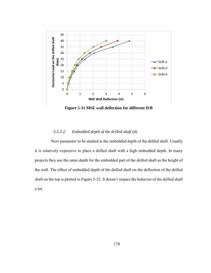
178
Figure 5-31 MSE wall deflection for different D/B
5.5.3.2. Embedded depth of the drilled shaft (d)
Next parameter to be studied is the embedded depth of the drilled shaft. Usually
it is relatively expensive to place a drilled shaft with a high embedded depth. In many
projects they use the same depth for the embedded part of the drilled shaft as the height of
the wall. The effect of embedded depth of the drilled shaft on the deflection of the drilled
shaft on the top is plotted in Figure 5-32. It doesn’t impact the behavior of the drilled shaft
a lot.
0
5
10
15
20
25
30
35
40
45
0 1 2 3 4 5 6
Ho
rizo
nta
l Lo
ad o
n t
he
dri
lled
sh
aft
(kip
s)
MSE Wall Deflection (in)
D/B=1
D/B=2
D/B=3

179
Figure 5-32 Drilled shaft deflection for different embedded depth
5.5.3.3. Backfill material
Most common backfill materials which are widely used for MSE walls are clean
sand and crushed rock. In this research the effect of these two materials on the interaction
between the drilled shaft and the MSE wall are studied.
Deflection of the drilled shaft and MSE wall for different backfill materials are
presented in Figure 5-33 and Figure 5-34. Deflection for both the MSE wall and the drilled
shaft is bigger for sand material.
0
5
10
15
20
25
30
35
40
45
0 2 4 6 8 10 12 14
Ho
rriz
on
tal L
oad
on
th
e D
rille
d S
haf
t (k
ips)
Drilled Shaft Deflection (in)
20 ft
15 ft
10 ft
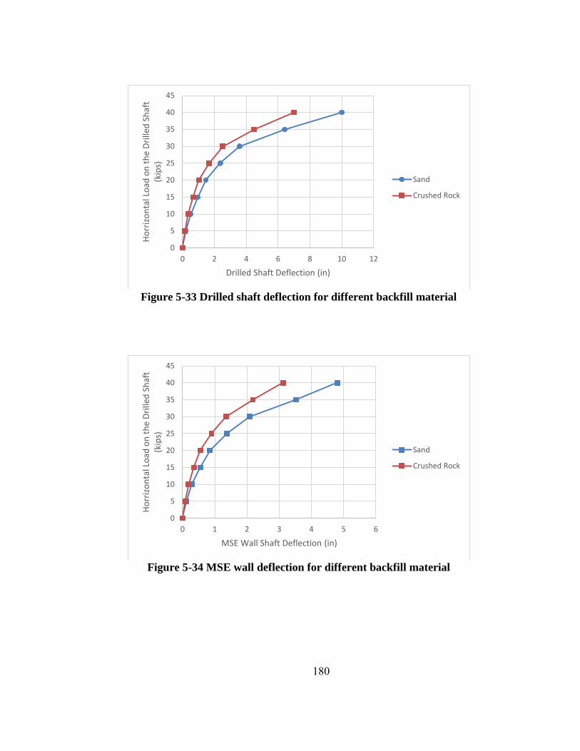
180
Figure 5-33 Drilled shaft deflection for different backfill material
Figure 5-34 MSE wall deflection for different backfill material
0
5
10
15
20
25
30
35
40
45
0 2 4 6 8 10 12
Ho
rriz
on
tal L
oad
on
th
e D
rille
d S
haf
t (k
ips)
Drilled Shaft Deflection (in)
Sand
Crushed Rock
0
5
10
15
20
25
30
35
40
45
0 1 2 3 4 5 6
Ho
rriz
on
tal L
oad
on
th
e D
rille
d S
haf
t (k
ips)
MSE Wall Shaft Deflection (in)
Sand
Crushed Rock

181
5.6. Conclusion
Numerical modeling was an important part of this research. Totally 64 3D
models for the MSE wall, 6 models for the pull-out test and 28 models for the actual strips
were conducted in this research. Wall deformation, drilled shaft deformation, stress in
strips at different positions and pressure on the back of the wall panels were obtained from
MSE wall models. The model parameters related to the soil reinforcements were
calculated from the strip pull-out test modeling. Behavior of the metal strips was looked
more closely by modeling the actual strip in 3D.

182
6. ANTICIPATED DESIGN METHOD
6.1. Introduction
This chapter presents the anticipated design method of Mechanically Stabilized
Earth (MSE) wall for the case in which there is drilled shaft behind the wall in the
reinforced zone. The design methods which are presented in many geotechnical codes and
handbooks are for the standard situation which there is no drilled shaft behind the wall.
One of the accredit codes which is widely used is AASHTO. The goal of this chapter is to
include the effect of the horizontally loaded drilled shaft on the design of the wall. This
modification is based on the results of the full-scale test completed at Riverside Campus
of Texas A&M University in August 2012 (chapter 4) monitoring of real project sites
(chapter 4), and numerous numerical models which were calibrated based on the test and
field data (chapter 5)
6.2. Design method without the drilled shaft
The internally stability of the MSE wall is addressed by pull-out capacity and
yield of the reinforcement (American Association of State Highway & Transportation
Officials. Subcommittee on Bridges, 2010) Pull-Out Design
6.2.1. Pull-out design
One of the possible failure mechanism in MSE wall is reinforcement pull-out.
The length of the reinforcement should be long enough to avoid this kind of failure.
Reinforcement length is consist of the length of failure zone in the depth of the
reinforcement (Lmax) and the required safe length of the reinforcement (La). Lmax for a rigid
wall is shown in Figure 6-1. The design requires knowledge of Lmax which is to be ignored

183
in the length required to resist maximum tension (Tmax) in the reinforcement (Briaud,
2013). The force Tmax is related to the pressure on the panel and calculated as follows:
m a x v h hT s s (6.1)
Where Tmax is the maximum tension to be resisted by the layer of reinforcement
at depth z, sv is the vertical spacing between reinforcement layers at depth z, sh is the
horizontal spacing between reinforcement at depth z, and σh is the total horizontal stress
at depth z.
Figure 6-1 Required length of strip in the failure zone
σh is calculated as:
h r o v hk (6.2)
h
h/2
h/2
Lmax
0.3h

184
Where kr is coefficient of earth pressure, σov is the total vertical pressure due to
backfill material and Δσh is horizontal pressure due to any surcharge on top of the wall.
The applied load on the reinforcement is Tmax which is calculated as mentioned
above. The length of reinforcement that can safely carry this load without pulling out of
the soil, is calculated by:
m a x2p u ll o u t a
T f b L
(6.3)
Where the fmax is the maximum shear stress that can be developed on both sides
of the interface between the reinforcement and the soil, b is the width of the reinforcement,
and La is length of the inclusion beyond Lmax. fmax is calculated as:
* 'm a x v
f F (6.4)
Where F* is the friction factor proposed by (American Association of State
Highway & Transportation Officials. Subcommittee on Bridges, 2010). σ'v is the vertical
effective stress on the reinforcement, and α is a scale factor taken as 1 for steel
reinforcement, 0.8 for geogrids and 0.6 for geotextile (Briaud, 2013).
The ultimate limit state for pull-out must be fit in:
1 m a x 1 2 m a x 2 p u ll o u tT T T
(6.5)
Where ϒ1 is the load factor for active earth pressure due to soil weight
(ϒ1=1.35), ϒ2 is the load factor for the active earth pressure due to any surcharge on top
of the wall (ϒ2=1.5), φ is the resistance factor (φ=0.9), Tmax1 is the part of the load in the
reinforcement due to the soil weight, Tmax2 is the part of the load in the reinforcement due

185
to any surcharge on top of the wall, and Tpull-out is the pull out resistance calculated in
Eq(6.3). The required safe length La of the reinforcement is calculated by:
'1 2
* '
( )
2r o v h v h
o v
k s sL a
F b
(6.6)
The total length of reinforcement is calculated by:
'1 2
m ax * '
( )0 .3
2r o v h v h
a
o v
k s sL L L h
F b
(6.7)
6.2.2. Yield of the reinforcement design
Another reason of the failure in MSE wall is reinforcement yielding or rupture.
The ultimate limit state for this situation is:
1 m a x 1 2 m a x 2 y ie ldT T T (6.8)
Where ϒ1 is the load factor for active earth pressure due to soil weight
(ϒ1=1.35), ϒ2 is the load factor for the active earth pressure due to any surcharge on top
of the wall (ϒ2=1.5), φ is the resistance factor (φ=0.75 for strips, 0.65 for grids and 0.9 for
geosynthetics) Tmax1 is the part of the load in the reinforcement due to the soil weight,
Tmax2 is the part of the load in the reinforcement due to any surcharge on top of the wall,
and Tyield is the load corresponding to the yield strength of the reinforcement.
6.3. MSE wall design the drilled shaft
As it was mention in previous section, the main factor in designing an MSE wall
is the pressure on the panels. Based on this pressure at different depth, the length of
reinforcement and arrangement of them are designed. This pressure is going to be
calculated and inserted in the design.

186
6.3.1. Parameters to be studied
The additional pressure on the panels is a factor of different parameters.
Parameters that have great impact on the pressure where discussed in chapter 5 (shown in
Figure 6-2). These parameters are discussed in this section.
h1
D B
H0
Backfill Material
h2
h
Bridge Deck
Figure 6-2 Parameters affecting on the pressure on the panel due to horizontal load
on the drilled shaft
6.3.1.1. Horizontal load on the drilled shaft (H0)
The most important factor that plays a great role in the additional pressure is the
horizontal load on the drilled shaft which is called H0 in this chapter. This load is
calculated during designing of the bridge. According to the design procedure provided by

187
TxDOT it is equal to 13.5 kips. In this research the range studied for the horizontal load
on the shaft is between zero and 40 kips to cover all kinds of possible bridge designs.
6.3.1.2. Clear distance between the wall and the drilled shaft (D)
The other important parameters on the additional pressure on the panel are the
clear distance between the wall and the drilled shaft (D). When the drilled shaft is far from
the wall, there is bigger deformation on the top of the drilled shaft but smaller pressure on
the panels.
6.3.1.3. Diameter of the drilled shaft (B)
The diameter of the drilled shaft (B) has a great impact on the pressure on the
panel but in real projects, because there is a small range for B and it is pretty the same in
most of the projects (3 ft), it mainly used for normalizing other parameters.
6.3.1.4. Height of the wall (h1)
As it will be discussed later in this chapter, the distribution of the additional
pressure on the wall is a triangle with the big side on top. The height of the wall plays two
important roles. One of them is on the pressure on the panels and the other one is on the
distribution of the pressure. The range of the wall height in this research (10-25 ft) covers
most of the walls in real projects.
6.3.1.5. Backfill material
Backfill material has a minor impact on the pressure on the panels. In real
projects mainly there are two kinds of backfill materials; crushed rock and clean sand. In
this research the additional pressure on the back of the wall is studied for these two kind
of backfill materials.

188
6.3.2. Numerical cases
In order to study the effect of each parameter on the pressure on the panels,
numerous numerical models were prepared in FLAC 3D. As it was discussed in the chapter
5, these models were calibrated with data from full-scale test at Riverside Campus at Texas
A&M University and the monitoring of the real project site at Bastrop. The parameters
used in this research are shown in Table 6-1 and accordingly totally 64 models were
prepared.
Table 6-1 Parameters used in numerical models
Horizontal Load on top of the drilled shaft (H0), kips 0, 5, 10, 15, 20, 25, 30, 35, 40
Diameter of the drilled shaft, ft 2, 3
Clear distance between the drilled shaft and the wall, ft 1, 3, 6, 8, 10, 12, 15
Height of the wall, ft 10, 15, 20, 25
Backfill material Sand: φ=30o and E=210 ksf, Crushed rock: φ=40o and E=2.1×10³ ksf
To normalize the parameters that are affecting on the additional pressure, two
new parameters are defined as follows:
a) Relative distance between the drilled shaft and the wall (D/B)
b) Equivalent pressure in front of the shaft which is calculated as H0/(Bh1)

189
Results from numerical models are summarized in four graphs which two of
them are for sand backfill material and two of them are for crushed rock backfill material.
Additional pressures on the panels due to horizontal load on the drilled shaft for
the backfill material of crushed rock for different relative displacement between the drilled
shaft and the wall (D/B) are presented in Figure 6-3. As it can be seen in this figure, the
relative displacement between the drilled shaft and the wall plays a great role on the
additional pressure on the panel. For the case with the drilled shaft near the wall, a great
percentage of the pressure in front of the drilled shaft is transferred to the wall. For all of
the horizontal loads in numerical models, the relation between the additional pressure on
the panel and the pressure in front of the drilled shaft is linear.
Another interesting data obtained from numerical study is the additional force
in the strip around the drilled shaft. The results for backfill material of crushed rock are
shown in Figure 6-4. This force is due to additional pressure on the panel.

190
Figure 6-3 Additional pressure on the panels due to different horizontal loads on
the drilled shaft for crushed rock
Figure 6-4 Additional force in the strip due to different horizontal loads on the
drilled shaft for crushed rock
Additional pressures on the panels due to horizontal load on the drilled shaft for
the backfill material of sand for different relative displacement between the drilled shaft
0
500
1000
1500
2000
0 500 1000 1500 2000 2500 3000Ad
dit
ion
al p
ress
ure
on
th
e w
all (
PSF
)
H0/Bh1(PSF)
D/B=0.5
D/B=1
D/B=2
D/B=3
D/B=4
D/B=5
0
500
1000
1500
2000
2500
3000
3500
4000
4500
0 10 20 30 40 50
Ad
dit
ion
al f
orc
e in
th
e st
rip
(lb
)
Horizontal load (kips)
D/B=0.5
D/B=1
D/B=2
D/B=3
D/B=4
D/B=5

191
and the wall (D/B) are presented in Figure 6-5. As it can be seen in this figure, the relative
displacement between the drilled shaft and the wall plays a great role on the additional
pressure on the panel. For the case with the drilled shaft near the wall, a great percentage
of the pressure in front of the drilled shaft is transferred to the wall. In this case for
horizontal loads less than 30kips, the relation between the additional pressure on the panel
and the pressure in front of the drilled shaft is linear.
Another interesting data obtained from numerical study is the additional force
in the strip around the drilled shaft. The results for backfill material of crushed rock are
shown in Figure 6-6. This force is due to additional pressure on the panel.
Figure 6-5 Additional pressure on the panels due to different horizontal loads on
the drilled shaft for sand
0
200
400
600
800
1000
1200
1400
0 1000 2000 3000Ad
dit
ion
al p
ress
ure
on
th
e w
all (
PSF
)
H0/Bh1(PSF)
D/B=0.5
D/B=1
D/B=2
D/B=3
D/B=4
D/B=5

192
Figure 6-6 Additional force in the strip due to different horizontal loads on the
drilled shaft for sand
6.3.3. Pressure distribution on the panels
The additional pressure on the back of the wall due to horizontal load on the
drilled shaft which was calculated above is the pressure on top of the wall. To have the
pressure on the entire wall, the distribution of pressure should be specified. In order to get
the distribution, the pressures on the back of the wall along the wall height are plotted for
different cases. Some of these plots are presented in this chapter.
Case 1: shaft diameter is 2ft, clear distance between the drilled shaft and the wall
is 2ft (D/B=1), height of the wall is 15ft, and the backfill material is sand. The additional
pressure along the wall height is shown in Figure 6-7. The additional pressure on top of
the wall is zero and it increase rapidly by increasing the depth.
0
500
1000
1500
2000
2500
3000
3500
0 10 20 30 40 50
Ad
dit
ion
al f
orc
e in
th
e st
rip
(lb
)
Horizontal load (kips)
D/B=0.5
D/B=1
D/B=2
D/B=3
D/B=4
D/B=5

193
Case 2: shaft diameter is 3 ft, clear distance between the drilled shaft and the
wall is 6ft (D/B=2), height of the wall is 20ft, and the backfill material is crushed rock.
The additional pressure along the wall height for this case is shown in Figure 6-8. The
outline of the pressure distribution is pretty the same as case 1.
Figure 6-7 Pressure distribution along the wall height for case 1
0
2
4
6
8
10
12
14
16
0 200 400 600 800 1000
Wal
l Hei
ght
(ft)
Additional Pressure (PSF)

194
Figure 6-8 Pressure distribution along the wall height for case 2
Case 3: shaft diameter is 3 ft, clear distance between the drilled shaft and the
wall is 9ft (D/B=3), height of the wall is 25ft, and the backfill material is sand. The
additional pressure along the wall height for this case is shown in Figure 6-9. The outline
of the pressure distribution is pretty the same as case 1 and case 2.
0
2
4
6
8
10
12
14
16
18
20
0 200 400 600
Wal
l Hei
ght
(ft)
Additional Pressure (psf)

195
Figure 6-9 Pressure distribution along the wall height for case 3
According to the additional pressure along the wall height obtained from
numerical models, the distribution of this additional pressure is in the form of a triangle
with the big side on top. The additional pressure calculated by this kind of distribution is
conservative on some part of the wall, especially at the bottom of the wall. Accordingly
all of the pressures on the back of the wall are shown in Figure 6-10 where krσov is the soil
pressure due to backfill material, Δσh is the pressure due to any surcharge at the top of the
wall and Δσs is the additional pressure due to horizontal load on the drilled shaft. By
having the additional pressure on top of the wall and wall height, additional pressure on
any depth can be calculated.
0
5
10
15
20
25
30
0 50 100 150 200
Wal
l Hei
ght
(ft)
Additional Pressure (psf)
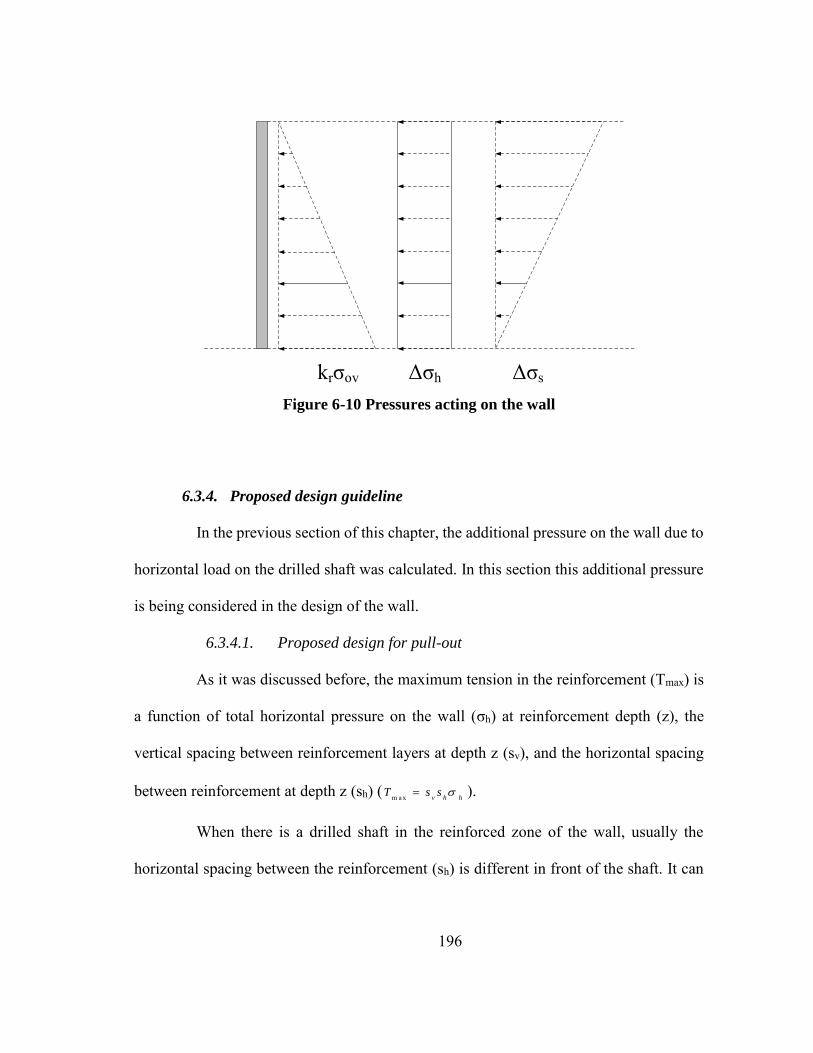
196
Figure 6-10 Pressures acting on the wall
6.3.4. Proposed design guideline
In the previous section of this chapter, the additional pressure on the wall due to
horizontal load on the drilled shaft was calculated. In this section this additional pressure
is being considered in the design of the wall.
6.3.4.1. Proposed design for pull-out
As it was discussed before, the maximum tension in the reinforcement (Tmax) is
a function of total horizontal pressure on the wall (σh) at reinforcement depth (z), the
vertical spacing between reinforcement layers at depth z (sv), and the horizontal spacing
between reinforcement at depth z (sh) ( m a x v h hT s s ).
When there is a drilled shaft in the reinforced zone of the wall, usually the
horizontal spacing between the reinforcement (sh) is different in front of the shaft. It can
krσov Δσh Δσs

197
be measured precisely from the wall drawing but for a good estimation sh in front of the
drilled shaft is one and half times sh in other part of the wall.
Another difference in the design when there is a horizontally loaded drilled shaft
in the wall is the total horizontal pressure on the panels in front of the wall. In this case a
new term is added to the Eq (6.2) and the new equation is as follows:
h r o v h sk (6.9)
Where Δσs is the additional pressure due to the horizontally loaded drilled shaft.
The new equation for calculating the required safe length (La) of the
reinforcement is:
'1 2 2
* '
( )
2r o v h v h
o v
k s s sL a
F b
(6.10)
And the total length of reinforcement is calculated by:
'1 2 2
m ax * '
( )0 .3
2r o v h v h
a
o v
k s s sL L L h
F b
(6.11)
As it was discussed before, the relation between the additional pressure (Δσs)
and the pressure in front of the drilled shaft (H0/Bh) is linear. The proposed chart to
calculate maximum Δσs is presented in Figure 6-11. It is prepared for two main backfill
materials used in MSE walls (sand and crushed rock). All of the parameters in the chart
can be obtained from the geometry (D, B, h) and design of the drilled shaft (H0) and the
additional pressure on the panels can be calculated.
Pressure on the wall according to “2 to 1” method is also plotted in Figure 6-11.
For the cases where the drilled shaft is far from the wall this method is conservative.

198
Figure 6-11 Proposed chart to calculate Δσs based on the geometry and applied
horizontal load on the shaft
6.3.4.2. Proposed design for rupture failure
The governing equation for rupture is 1 m a x 1 2 m a x 2 y ie ldT T T . If we consider
the additional pressure due to the horizontal load, the proposed equation for rupture is:
'1 2 2( )
r ov h v h yieldk s s s T (6.12)
6.3.4.3. Check wall panel for bending
The additional pressure due to the horizontal load on the drilled shaft is acting
on the panels and panel reinforcement should be checked for the maximum bending on
the panel. Detail of the panels is presented in Figure 6-12. Additional pressure is bigger
on the top of the wall so the most critical panel is the one at the top of the wall.
0
0.1
0.2
0.3
0.4
0.5
0.6
0.7
0.8
0 1 2 3 4 5
𝛥𝜎𝑠m
ax/(𝐻
0/𝐵ℎ
)
D/B
Sand
Crushed Rock
2 to 1 method

199
Figure 6-12 Panel details
The design for the panel at Bastrop project site including the additional pressure
is presented here:

200
'
y
2m a x
M a x im u m s p a n : 2 .5 f t
S la b th ic k n e s s ( t) = 5 .5 in
A d d it io n a l P re s s u re : 7 3 .3 1 p s f
C o n c re te f 4 0 0 0
S te e l f = 6 0 0 0 0
A t in te r io r s p a n : M 1 / 9 1 .5 7 3 .3 1 2 .5 7 6 .4
C o v e r o f th e re in fo rc e m e n t = 1 in
1
c
lb f t
d t
2m a x
4 .5
7 6 .4 1 2A 0 .0 0 4 2
0 .9 6 0 0 0 0 4( )2
s
y
Min
af d
Minimum reinforcement used in the panels are:
2m in 0 .0 0 1 8 0 .0 0 1 8 ( 2 .5 1 2 ) 4 .5 0 .2 4 3
sA b d in
6.4. Comparison between AASHTO design and proposed design
Here is the comparison between the AASHTO design and the new design of the
wall in Bastrop project based on the proposed design guideline:
Project specification: height of the wall (h) is 18ft, diameter of the drilled shaft
(B) is 3ft, clear distance between the drilled shaft and the wall (D) is 6ft (D/B=2),
Horizontal (Sh) and vertical (sv) spacing of the reinforcements are both 2.5ft, and backfill
material is crushed rock with unit weight of 120pcf
kr is assumed to be equal to ka which is 0.33, F* at the top of the wall is 1.7, scale
factor (α) is 1.0, and the width of the strip is 0.16ft. The calculation is for second row of
strips from the top at the depth of 3ft from the top of the wall.

201
18ft
6ft 3ft
15 kips
Backfill Material
3ft
21ft
Bridge Deck
3ft
Figure 6-13 Detail of the wall
AASHTO design method
(1 .3 5 0 .3 3 1 2 0 3) 2 .5 2 .55 .7
2 0 .9 1 .7 1 2 0 3 1 0 .1 6a
L ft
0 .3 5 .7 5 .4 1 1 .1L L a h ft
The required length of strip is 11.2ft and the length of strip used in the project at
that level is 18ft.
Proposed design method
The designed horizontal load on the drilled shaft (H0) for this project is 15kips.
0 1 5 0 0 02 7 8
7 3 .3 13 1 8
/ 2s
H
p s fB h
D B

202
The additional pressure calculated above is for the top of the triangle, so the
additional pressure at the second row of strips at the depth of three is
1 57 3 .3 1 6 1 .0 9
1 8p s f .
The other point that should be consider is the horizontal spacing of the strips in
front of the drilled shaft which in this case is1 .5 3 .7 5h
s f t . So the required length of
the strip according to the proposed design guideline is:
(1 .3 5 0 .3 3 1 2 0 6 1 .5 6 1 .0 9 ) 2 .5 1 .5 2 .51 1 .0
2 0 .9 1 .7 1 2 0 6 1 0 .1 6a
L ft
0 .3 1 1 5 .4 1 6 .4L L a h ft
In this project the length of the strips is enough to carry the horizontal pressure
on the panel, including the additional pressure due to the horizontal load on the drilled
shaft. This project is being monitored since December 2013 and so far there has been no
problem. Different lengths of strips for different D/B are presented in Table 6-2.
Table 6-2 Length of strip for different D/B
D/B 𝛥𝜎𝑠/(𝐻0/𝐵ℎ) 𝛥𝜎𝑠 (top)
(psf)
𝛥𝜎𝑠 (at strip level)
(psf) La (ft) 0.3h (ft) L (ft)
Increase %
0 0 0 0 5.70 5.40 11.10 0.00
0.5 0.71 197.35 164.46 15.09 5.40 20.49 84.61
1 0.54 149.68 124.73 13.51 5.40 18.91 70.33
2 0.26 73.31 61.09 10.97 5.40 16.37 47.46
3 0.15 40.78 33.99 9.89 5.40 15.29 37.71
4 0.10 27.63 23.03 9.45 5.40 14.85 33.78
5 0.04 10.79 8.99 8.89 5.40 14.29 28.73

203
6.5. General considerations
Moreover to what discussed above, there are some construction suggestions that
can reduce the failure risk of the MSE wall with a horizontally loaded drilled shaft behind
it. In this part these suggestions are being discussed.
a) Put the drilled shaft as far as possible from the wall.
As it can be seen in Figure 6-11, there is more pressure transferred to the wall
when the drilled shaft is near the wall. The other problem is when the space between the
drilled shaft and the wall is limited, the soil in between cannot be compacted which may
decrease the friction factor (F*) of the strips and in some cases results in strip pull-out.
b) Compact the soil between the drilled shaft and the wall.
The compaction plays an important role in the friction factor on the strips. The
better compaction is done, the greater load can be carried by the strips. In cases where the
drilled shaft is very close to the wall, the soil in between cannot be compacted with
compaction machine. In these cases it is highly recommended to compact the soil by hand.
c) Put the drilled shaft in front of the center of the panel especially at the top of the
wall.
The additional pressure due to the horizontal load on the drilled shaft is bigger
at the top of the wall. So it is better if this pressure be carried by the panel not the shear
keys between the panels. In some failure cases of the MSE walls, the failure occurred at
the shear keys at the top of the wall.
d) Decrease the spacing of the strips if necessary.

204
Sometimes it is hard to increase the length of the strips due to space restrictions
at the site. In these cases if it is necessary to increase the length of the strips due to the
additional pressure, it is recommended to decrease the spacing of the strips especially the
vertical spacing (sv).
6.6. Conclusion
The interaction between the drilled shaft and the MSE wall results in an
additional pressure on the back of the wall panels. This additional pressure is a functional
geometry of the wall and the drilled shaft and also the backfill material.
This pressure is has a triangular distribution with the big side on top (Δσsmax).
By knowing this pressure and the depth of strips, the additional pressure at each level can
be found and the required length of strip at each level can be calculated.

205
7. CONCLUSIONS AND PROPOSAL FOR FUTURE WORKS
7.1. Summary and conclusions
The current design guidelines for MSE walls do not consider the interaction
between MSE wall and drilled shafts. This Thesis is aimed at addressing this particular
problem. There are other research efforts in this field, but they are related to MSE walls
using geosynthetics and geogrid as reinforcements. However, no changes in the guidelines
were proposed after those investigations. Furthermore, in Texas the MSE walls are
generally constructed using metallic reinforcements. . Therefore, an investigation that
combines laboratory tests, in-situ experiments, monitoring of MSE wall under actual
conditions and numerical modeling was undertaken in this Thesis to advance the current
knowledge in this area with the explicit aim of suggesting modification in the current
guidelines to incorporate the interaction between MSE wall and drilled shaft in the design
of this earthwork structures.
To study the problem in more detail, a full-scale test and the monitoring of two
actual sites were designed in this Thesis. The design of the instrumentation was done with
the aim of gathering the most relevant information from full-scale loading test at Riverside
campus and the monitoring from two actual sites. The maximum number of sensors was
based on the number of channel available on data loggers to collect data. As for the full-
scale test, two data loggers were used, with a total of 20 channels were used to gather the
data. As for the monitoring at the actual TxDOT sites, one data logger used for each site
and 15 channels were used to gather the data. The types of devices were selected according
to the required precision and durability. Durable devices were needed especially for

206
monitoring the actual TxDOT sites, because they were designed to gather t data for around
16 months.
The full-scale test was performed successfully at Riverside Campus at Texas
A&M University. All of the devices worked perfectly during the test and valuable data
was gathered from this test. The test took about 4 hours to perform and 19 people were
involved in the test with the PhD candidate leading it. After the test it was confirmed that
the stress in the second layer of strips (from the top) is greater than the top layer. Also the
highest stress in the strip occurred at 25 kips of horizontal load and after that the stress
was reduced. The MSE wall and shaft deformation were other important data which were
gathered in this test that helped the writer to calibrate numerical models.
The TxDOT project at the site in Bastrop, Texas, was monitored for six months.
All of the devices were installed on the wall and drilled shaft during the construction
phase. The data has been gathered since the bridge was opened to traffic. The initial plan
was to monitor this project site for 16 months, but due to contraction delays, the
monitoring period has been reduced to six months. No big movement or increase in the
stress and pressure were observed during the monitoring. The monitoring of this site will
continue after this thesis. In the other TxDOT site located in Salado, Texas, the
instrumentation was installed and it is ready to collect the data, however due to
construction delay no data was gathered from this site yet.
Numerical modeling was an important component of this research. A number of
numerical models were prepared to study the behavior of the MSE wall and shat and other
ones focused on the study of the metal strip in detail. A total of 64 models for the MSE

207
wall, 6 models for the pull-out tests, and 28 models for the actual strips were conducted in
this research. Wall deformation, drilled shaft deformation, stress in strips at different
positions and pressure on the back of the wall panels were obtained from the MSE wall
models. The model parameters related to the soil reinforcements were calculated from the
strip pull-out test modeling. Behavior of the metal strips was looked more closely by
modeling the actual strip in 3D. In this section the effect of each parameter was studied
and two main parameters were introduced that plays an important role in this research.
First one is the relative displacement which is the clear distance between the drilled shaft
and the wall (D/B), and the second one is the equivalent pressure in front of the drilled
shaft that is the horizontal load on the shaft divided by diameter of the shaft times height
of the MSE wall (H0/(Bh1)).
The effect of horizontally loaded drilled shaft behind the MSE wall is an
additional pressure on the back of the wall panels. This additional pressure is a function
of the geometry of the wall and the drilled shaft and also the backfill material. This
pressure has a triangular distribution in depth, with the larger pressure on the top (Δσsmax).
In this Thesis is proposed that by knowing this maximum pressure and the depth of the
strips, the additional pressure at each level can be found. From this additional pressure the
required length of the strip at each level can be calculated.
7.2. Proposal for future works
There are still many different problems related to the behavior of MSE walls that
need attention and to address them can be a great help for designers and contractors. Some

208
aspects that can contribute to a better understanding of the MSE wall behavior and its
design are discussed below
The study of the effect of other backfill materials on the interaction:
Backfill materials which were used in in this research, are clean sand and
crushed rock because these are the two most common backfill materials for MSE walls in
Texas. Study the effect of fine grain materials on the interaction would be very interesting.
Isolate the drilled shaft from the wall: to avoid the additional pressure due to the
drilled shaft on the wall panels, the drill shaft can be isolated from the backfill material,
or another type of material can be used between the drilled shaft and the MSE wall to
reduce the amount of the pressure on the panels.
Redesign the metal strips: metal strip is a very interesting kind of soil
reinforcements because of the high friction factor. This friction factor is related to the
bumps on the strips and is a function of the number of bums and their geometry. The best
combination of the bump numbers and geometry can be designed in order to obtain the
maximum friction factor by doing some pull-out test and numerical modeling. This will
results in shorter strips in the wall and more economical and very likely safer design.

209
REFERENCES
Abdelouhab, A., Dias, D., & Freitag, N. (2011). Numerical analysis of the behaviour of
mechanically stabilized earth walls reinforced with different types of strips.
Geotextiles and Geomembranes, 29(2), 116-129.
Ahmadabadi, M., & Ghanbari, A. (2009). New procedure for active earth pressure
calculation in retaining walls with reinforced cohesive-frictional backfill.
Geotextiles and Geomembranes, 27(6), 456-463.
American Association of State Highway, & Transportation Officials. Subcommittee on
Bridges. (2010). AASHTO load and resistance factor design movable highway
bridge design specifications. Washington, D.C.: AASHTO.
Arenas, A. E. (2010). Thermal response of integral abutment bridges with mechanically
stabilized earth walls. ( No. VCTIR 13-R7). Charlottesville, VA: Virginia Center
for Transportation.
ASTM D1557-12. (2012). Standard test methods for laboratory compaction
characteristics of soil using modified effort. West Conshohocken, PA: ASTM.
Bathurst, R. J., Nernheim, A., & Allen, T. M. (2009). Predicted loads in steel reinforced
soil walls using the AASHTO simplified method. Journal of Geotechnical and
Geoenvironmental Engineering, 135(2), 177-184.

210
Berg, R., & Vulova, C. (2007). Effects of pile driving through a full-height precast
concrete panel faced, geogrid-reinforced, mechanically stabilized earth (MSE) wall.
Proc., Sessions of Geo-Denver 2007, ASCE Geotechnical Special Publication No,
159
Berg, R. R., Christopher, B. R., & Samtani, N. C. (2009). Design of mechanically
stabilized earth walls and reinforced soil slopes–Volume II. ( No. FHWA GEC 011-
Vol II). Washington, D.C.: FHWA.
Bergado, D. T., Lo, K., Chai, J., Shivashankar, R., Alfaro, M. C., & Anderson, L. R.
(1992). Pullout tests using steel grid reinforcements with low-quality backfill.
Journal of Geotechnical Engineering, 118(7), 1047-1062.
Bergado, D. T., & Teerawattanasuk, C. (2008). 2D and 3D numerical simulations of
reinforced embankments on soft ground. Geotextiles and Geomembranes, 26(1), 39-
55.
Briaud, J. (1992). The pressuremeter. Rotterdam, Netherlands: Taylor &
Francis/Balkema.
Briaud, J. (2013). Geotechnical engineering: Unsaturated and saturated soils. Hoboken,
NJ: John Wiley & Sons.

211
Chen, D., Nazarian, S., & Bilyeu, J. (2007). Failure analysis of a bridge embankment
with cracked approach slabs and leaking sand. Journal of Performance of
Constructed Facilities, 21(5), 375-381.
Christopher, B. R., Gill, S. A., Giroud, J., Juran, I., Mitchell, J. K., Schlosser, F., &
Dunnicliff, J. (1990). Reinforced soil structures volume I.design and construction
guidelines. ( No. FHWA-RD-89-043). Washington, D.C.: US Department of
Transportation, Federal Highway Administration.
Elias, V., Barry, P., & Christopher, R. (1997). Mechanically stabilized earth walls and
reinforced soil slopes design and construction guidelines: FHWA demonstration
project 82, reinforced soil structures WSEW and RSS. Washington, D.C.: US
Department of Transportation, Federal Highway Administration.
Gerber, T. M., & Cummins, C. R. (2009). Modeling and analysis to quantify MSE wall
behavior and performance. ( No. UT-10.03). Salt Lake City, UT: Utah Department
of Transportation.
Hatami, K., & Bathurst, R. J. (2005). Development and verification of a numerical
model for the analysis of geosynthetic-reinforced soil segmental walls under
working stress conditions. Canadian Geotechnical Journal, 42(4), 1066-1085.
Hossain, M., Kibria, G., Khan, M., Hossain, J., & Taufiq, T. (2011). Effects of backfill
soil on excessive movement of MSE wall. Journal of Performance of Constructed
Facilities, 26(6), 793-802.

212
Huang, B., Bathurst, R. J., & Hatami, K. (2009). Numerical study of reinforced soil
segmental walls using three different constitutive soil models. Journal of
Geotechnical and Geoenvironmental Engineering, 135(10), 1486-1498.
Huang, J., Han, J., Parsons, R. L., & Pierson, M. C. (2013). Refined numerical modeling
of a laterally-loaded drilled shaft in an MSE wall. Geotextiles and Geomembranes,
37, 61-73.
Huang, J., Parsons, R. L., Han, J., & Pierson, M. (2011). Numerical analysis of a
laterally loaded shaft constructed within an MSE wall. Geotextiles and
Geomembranes, 29(3), 233-241.
Itasca. (2006). Fast lagrangian analysis of continua in 3-dimensions, version 4.0,
manual. Minneapolis, MN: Itasca.
Jewell, R. A. (1980). Some effects of reinforcement on the mechanical behaviour of
soils. (Doctoral, University of Cambridge).
Johnson, A. P. (2013). Pullout resistance of mechanically stabilized earth
reinforcements embedded in coarse backfill and measured in a large scale test
system. (). Lubbock, TX: Texas Tech University.
Khodair, Y. A., & Hassiotis, S. (2005). Analysis of soil–pile interaction in integral
abutment. Computers and Geotechnics, 32(3), 201-209.

213
Kibria, G., Hossain, M. S., & Khan, M. S. (2013). Influence of soil reinforcement on
horizontal displacement of MSE wall. International Journal of Geomechanics,
14(1), 130-141.
Koerner, R. M., & Soong, T. (2001). Geosynthetic reinforced segmental retaining walls.
Geotextiles and Geomembranes, 19(6), 359-386.
Laefer, D. F., Fitzgerald, M., Maloney, E. M., Coyne, D., Lennon, D., & Morrish, S. W.
(2009). Lateral image degradation in terrestrial laser scanning. Structural
Engineering International, 19(2), 184-189.
Lawson, W. D., Jayawickrama, P. W., Wood, T. A., & Surles, J. G. (2013). Pullout
resistance factors for inextensible MSE reinforcements embedded in sandy backfill.
Paper presented at the Transportation Research Board 92nd Annual Meeting, (13-
2684)
Leshchinsky, D., Vahedifard, F., & Leshchinsky, B. A. (2012). Revisiting bearing
capacity analysis of MSE walls. Geotextiles and Geomembranes, 34, 100-107.
Miyata, Y., & Bathurst, R. J. (2012). Measured and predicted loads in steel strip
reinforced< i> c−< i> ϕ soil walls in japan. Soils and Foundations, 52(1), 1-17.
Pierson, M. (2008). Behavior of laterally loaded shafts constructed behind the face of a
mechanically stabilized earth block wall. Ann Arbor, MI: ProQuest.

214
Pierson, M. C., Parsons, R. L., Han, J., & Brennan, J. J. (2010). Laterally loaded shaft
group capacities and deflections behind an MSE wall. Journal of Geotechnical and
Geoenvironmental Engineering, 137(10), 882-889.
Pierson, M. C., Parsons, R. L., Han, J., Brown, D., & Thompson III, W. R. (2009).
Capacity of laterally loaded shafts constructed behind the face of a mechanically
stabilized earth block wall. ( No. K-TRAN: Ku-07-6). Topeka, KS: Kansas
Department of Transportation.
Stuedlein, A. W., Bailey, M., Lindquist, D., Sankey, J., & Neely, W. J. (2010). Design
and performance of a 46-m-high MSE wall. Journal of Geotechnical and
Geoenvironmental Engineering, 136(6), 786-796.
Suksiripattanapong, C., Chinkulkijniwat, A., Horpibulsuk, S., Rujikiatkamjorn, C., &
Tanhsutthinon, T. (2012). Numerical analysis of bearing reinforcement earth (BRE)
wall. Geotextiles and Geomembranes, 32, 28-37.
Tanchaisawat, T., Bergado, D., & Voottipruex, P. (2008). Numerical simulation and
sensitivity analyses of full-scale test embankment with reinforced lightweight
geomaterials on soft bangkok clay. Geotextiles and Geomembranes, 26(6), 498-511.
Yoo, C., & Kim, S. (2008). Performance of a two-tier geosynthetic reinforced segmental
retaining wall under a surcharge load: Full-scale load test and 3D finite element
analysis. Geotextiles and Geomembranes, 26(6), 460-472.

215
Zhou, W., Yin, J., & Hong, C. (2011). Finite element modelling of pullout testing on a
soil nail in a pullout box under different overburden and grouting pressures.
Canadian Geotechnical Journal, 48(4), 557-567.