Integrated Tool Development for Used Fuel Disposition … Integrated... · for Used Fuel...
133
Integrated Tool Development for Used Fuel Disposition Natural System Evaluation – Phase I Report Prepared for U.S. Department of Energy Used Fuel Disposition Yifeng Wang & Teklu Hadgu Sandia National Laboratories Scott Painter, Dylan R. Harp & Shaoping Chu Los Alamos National Laboratory Thomas Wolery Lawrence Livermore National Laboratory Jim Houseworth Lawrence Berkeley National Laboratory September 28, 2012 FCRD-UFD-2012-000229 SAND2012-7073P
Transcript of Integrated Tool Development for Used Fuel Disposition … Integrated... · for Used Fuel...

Integrated Tool Development
for Used Fuel Disposition
Natural System Evaluation –
Phase I Report
Prepared for U.S. Department of Energy
Used Fuel Disposition Yifeng Wang & Teklu Hadgu
Sandia National Laboratories Scott Painter, Dylan R. Harp & Shaoping Chu
Los Alamos National Laboratory Thomas Wolery
Lawrence Livermore National Laboratory Jim Houseworth
Lawrence Berkeley National Laboratory September 28, 2012
FCRD-UFD-2012-000229 SAND2012-7073P

DISCLAIMER
This information was prepared as an account of work sponsored by an
agency of the U.S. Government. Neither the U.S. Government nor any
agency thereof, nor any of their employees, makes any warranty, expressed
or implied, or assumes any legal liability or responsibility for the accuracy,
completeness, or usefulness, of any information, apparatus, product, or
process disclosed, or represents that its use would not infringe privately
owned rights. References herein to any specific commercial product,
process, or service by trade name, trade mark, manufacturer, or otherwise,
does not necessarily constitute or imply its endorsement, recommendation,
or favoring by the U.S. Government or any agency thereof. The views and
opinions of authors expressed herein do not necessarily state or reflect
those of the U.S. Government or any agency thereof.
Sandia National Laboratories is a multi-program laboratory managed and
operated by Sandia Corporation, a wholly owned subsidiary of Lockheed
Martin Corporation, for the U.S. Department of Energy‘s National Nuclear
Security Administration under contract DE-AC04-94AL85000.

Integrated Tool Development for UFD Natural System Evaluation
9/1/2012 iii

Integrated Tool Development for UFD Natural System Evaluation
iv 9/1/2012

Integrated Tool Development for UFD Natural System Evaluation
9/1/2012 v
Executive Summary
The natural barrier system (NBS) is an integral part of a geologic nuclear waste repository. From a
generally accepted multiple barrier concept, each barrier is supposed to be utilized for its safety function
independently to its optimal extent. In this sense the NBS needs to be evaluated and necessary research
conducted to ensure its optimal safety function. As one of its main objectives, the natural system
evaluation and tool development package will ensure that sufficient research will be conducted to fully
exploit the credits that can be taken for the NBS.
The work documented in this report is aimed to develop an integrated modeling framework that can be
used for systematically analyzing the performance of a natural barrier system and identifying key factors
that control the performance of the system. This framework is designed as an integrated tool for
prioritization and programmatic decisions of UFDC natural system R&D activities, and it includes three
key components: (1) detailed process models (with appropriate levels of fidelity) for flow field and
radionuclide transport, (2) a probabilistic performance assessment capability, and (3) an associated
technical database supporting model calculations. The integrated tool development for natural system
evaluation adopts a phased approach. This report documents the results of phase I activities, which are
focused on identifying relevant tools for subsystem analyses and performing preliminary demonstrations.
Major FY12 accomplishments are summarized as follows:
Two separate modeling frameworks were explored using different combinations of process
simulators and performance assessment drivers: (1) PFLOTRAN + PEST and (2) FEHM +
DAKOTA. Their preliminary application to flow and radionuclide transport in fractured granite
and dolomite media was demonstrated using Monte-Carlo simulations. The potential application
of a ―plug-and-play‖ concept, common data format, and high performance computing techniques
were explored.
Calibration-constrained uncertainty analyses were performed for a flow field in a hypothetical
fractured granite medium using PFLOTRAN and PEST.
The modeling frameworks were demonstrated to be able to incorporate or use real field data
(transmissivity fields), the dual-porosity capability of transport code (FEHM), the high
performance parallel computing capability of PA driver (DAKOTA), and the embedded LHS
sampling and statistical analysis techniques (DAKOTA).
A comprehensive review of thermodynamic data relevant to nuclear waste disposal was
performed, and the related data gaps were identified, especially for layered aluminosilicates.
A comprehensive literature survey and data compilation were performed for modeling the near-
field thermal-hydrological-mechanical-chemical evolution of a clay repository and for modeling
flow and radionuclide transport in a fractured granite medium. These data will be used to develop
an appropriate data model for UFDC data management.
Future work will include:
Move the integrated tool development from phase I into phase II by merging the existing two
separate modeling frameworks into a single integrated framework.
Develop the capability to incorporate an advanced flow-transport model for fractured geologic
media, such as a discrete fracture network (DFN) flow model, into the framework.
Continue to explore and demonstrate the capability of model parameter estimation and
uncertainty analyses using the established framework.
Continue data collection and synthesis to establish a comprehensive technical database for natural
system evaluation.

Integrated Tool Development for UFD Natural System Evaluation
vi 9/1/2012

Integrated Tool Development for UFD Natural System Evaluation
9/1/2012 vii
Table of Contents
1.0 Development of Integrated Tools for UFD Natural System Evaluation: An
Introduction
1
1.1 Objectives 1
1.2 Technical Approach 2
1.3 Structure of This Report 3
1.4 Reference 4
2.0 Development of an Integrated Process Modeling Framework for
Performance Assessments of Natural Barrier Systems
5
2.1 Introduction 5
2.2 Design Considerations for a Next-Generation PA framework 5
2.2.1 Uncertainty and sensitivity analysis 6
2.2.2 File formats 8
2.3 Concept for a Generic Granitic Repository and Associated Assessment Framework 9
2.4 Tool Demonstration 11
2.4.1 Synthetic example 11
2.4.2 Workflow 13
2.4.3 Storage and organization 17
2.5 Example Assessment 17
2.6 Conclusions 25
2.7 References 26
3.0 Integrated Tool Development for Far-Field Radionuclide Transport in a Salt
Repository
28
3.1 Introduction 28
3.2 Generic Salt Repository and Model Setup 30
3.2.1 Description of FEHM Reservoir Simulator 30
3.2.2 Description of DAKOTA 31
3.2.4 Parallel version of DAKOTA-FEHM 32
3.3 Tool Demonstration 33
3.3.1 Flow simulations 34
3.3.2 Deterministic transport simulations 41
3.3.3 Probabilistic transport simulations 45
3.3.3.1 Simulations of iodine transport 46
3.3.3.2 Simulations of PU(IV) transport 52
3.3.3.3 Simulations of U(VI) transport 58
3.4 Summary 63
3.5 References 63
4.0 Disposal Systems Material Properties: Thermodynamic Data Collection and
Synthesis
65
4.1 Introduction 65
4.2 Uses of Thermodynamic Data in Repository Studies 66
4.3 Types of Thermodynamic Data 67
4.4 Issues with Thermodynamic Data: General 69
4.5 Sources of Thermodynamic Data 70
4.6 Data Gaps 71

Integrated Tool Development for UFD Natural System Evaluation
viii 9/1/2012
4.7 A Key Data Issue: The Entropies of the Chemical Elements in Their Reference Forms 76
4.8 A Core Data Issue: Thermodynamic Data for Aluminosilicate Minerals 80
4.9 Data Management Requirements 82
4.10 Data Management Records 85
4.11 References 85
5.0 Compilation of Key Technical Data for the Evaluation of Generic Disposal
Environments
90
5.1 Introduction 90
5.2 Data for THMC Modeling of the Near Field of a Clay Repository 90
5.2.1 Hydrologic Model 91
5.2.2 Mechanical Model 93
5.2.3 Chemical Model 95
5.2.4 Thermal Model 102
5.2.5 Non-Environment-Specific Parameters 103
5.3 Data for Modeling Granite Far Field Flow and Transport 103
5.4 References 120
6.0 Summary and Future Work 125

Integrated Tool Development for UFD Natural System Evaluation
9/1/2012 1
1.0 Development of Integrated Tools for UFD Natural
System Evaluation: An Introduction
1.1 Objectives
The natural barrier system is an integral part of a geologic nuclear waste repository. Spatially, it extends
from a so-called disturbed rock zone, created by mechanical, thermal and chemical perturbations due to
underground excavation or waste emplacement, to the surrounding geologic media, and continues all the
way to a specified repository boundary. The work package of natural system evaluation and tool
development supports the following Used Fuel Disposition Campaign (UFDC) objectives (Nutt, 2011):
1. Develop a fundamental understanding of disposal system performance in a range of environments
for potential wastes that could arise from future nuclear fuel cycle alternatives through theory,
simulation, testing, and experimentation.
2. Develop a computational modeling capability for the performance of storage and disposal options
for a range of fuel cycle alternatives, evolving from generic models to more robust models of
performance assessment.
From a well-accepted multiple barrier concept for waste repository safety, each barrier is to be
independently utilized for its safety function to its optimal extent. In this sense the natural barrier needs
to be evaluated and necessary research conducted to ensure its optimal safety function. From a repository
design point of view, an appropriate balance must be maintained between the natural barrier system
(NBS) and the engineered barrier system (EBS) in the contribution to the total system performance. In
practice, there is a risk to place too much reliance on the engineered barrier while not fully taking credits
for the natural system. Such practice often results in an overly conservative, very expensive EBS design.
Thus, as one of its main objectives, the natural system evaluation and tool development package will
ensure that sufficient research will be conducted to fully exploit the credits that can be taken for the NBS.
In FY11, a detailed research plan was developed for the NBS evaluation and tool development (Wang,
2011). In that plan, a total of 27 key research topics were identified. The effort on the integrated tool
development for natural system evaluation tends to address the following three topics:
Topic #S2. Disposal concept development: As explicitly identified in the UFDC Research &
Development (R&D) roadmap (Nutt, 2011), there is a need for developing a range of generic
disposal system design concepts. This research topic will support the overall UFDC effort on the
development of disposal system design concepts by cataloging possible combinations and
geometries of both host rock and far-field media (e.g., mineral and chemical compositions,
physical dimensions, hydrologic properties). The topic will include the definition a generic set of
key parameters (e.g., water chemistry) for other UFDC activities.
Topic #S3. Disposal system modeling: Disposal system modeling is crucial for the whole life
cycle of repository development. Such modeling tools will be essential for management
decisions on project priority and resource allocation. This research will serve two purposes: (1)
supporting the development of the total system performance assessment as well as the
development of higher-fidelity performance assessment models, and (2) developing a
comprehensive subsystem model for natural system performance evaluation. This subsystem
model will be used for integration and prioritization of relevant natural system evaluation
activities.

Integrated Tool Development for UFD Natural System Evaluation
2 9/1/2012
Topic #S4. Development of a centralized technical database for natural system evaluation: Given
the quantity of data already accumulated through various repository programs and also the data to
be collected from the UFDC R&D activities, it is essential for future repository development to
archive and categorize these data in an appropriate manner so that they can be easily accessible to
UFDC participants and have appropriate quality assurance enforced. The data to be collected will
include thermodynamic data for radionuclide speciation and sorption, groundwater chemistry,
hydraulic and mechanical property data, mineralogical and compositional data of representative
host and far-field media, spatial distributions of potential host formations, etc.
It is envisioned that the tools developed in this effort will be used to systematically analyze the
performance of a NBS and identify key controlling factors through sensitivity analyses and then be used
as an integration tool for prioritization and programmatic decisions of NBS-related R&D activities.
1.2 Technical Approach
The integrated tool development for NBS evaluation follows a probabilistic approach, similar to the one
developed for a total system performance assessment (TSPA) (Helton et al., 1999). This effort focuses on
the development a modeling framework that will include three key components: (1) detailed process
models (with appropriate levels of fidelity) for flow field and radionuclide transport calculations, (2)
probabilistic performance assessment capabilities, and (3) an associated technical database supporting
model analyses (Figure 1-1). In this framework, one or more detailed process models may be linked and
wrapped by a probabilistic performance assessment driver (PPAD). The PPAD then drives probabilistic
performance assessment calculations by sampling uncertain model input parameters and invoking Monte-
Carlo simulations using the linked process model(s). It is important for the modeling framework to be
flexible enough to accommodate various alternative models. This can be done through a plug-and-play
technique.
Figure 1-1. Integrated modeling framework for UFDC Natural Barrier System Evaluation
Probabilistic Performance
Assessment driver
Technical databaseProcess model 1 Process model 2

Integrated Tool Development for UFD Natural System Evaluation
9/1/2012 3
Given typical dimensions of the NBS and the level of process model details that may be needed for a
meaningful subsystem evaluation, a probabilistic performance assessment of a NBS may be
computationally intensive. To facilitate these calculations, we need to leverage recently developed high
performance computing techniques. Specifically, we need to explore the parallelization of process-level
codes and the parallel work assignment of sequential codes. The latter is important, because many legacy
codes for flow and transport in a far field of a repository are not parallelized.
The integrated tool development adopts a phased approach. In phase I, relevant tools will be identified
and preliminary demonstration will be performed. In phase II, the tools identified in phase I will be
aggregated into a single coherent framework and its function as an integrated tool will be preliminarily
demonstrated. In phase III, the established framework will be ready to support a comprehensive analysis
of a NBS. This report documents the work completed for phase I in FY12.
As mentioned above, the methodology adopted for this effort may resemble, in many aspects, to that used
for a TSPA. However, there are two significant distinctions between them in terms of the level of model
fidelity and the use of process models. First of all, our effort here focuses on the performance evaluation
of a NBS, not on a total disposal system. For this purpose, the process models to be used for this effort
for natural system flow and transport calculations are much more detailed than those used for a TSPA
calculation, and at the same time, for simplicity, only a stylized source term is used to represent
radionuclide release from a EBS to its surrounding NBS. Second, the NBS tool development pays specific
attention to the parameter estimation and uncertainty quantification using inverse process models.
Despite these distinctions, we are fully aware that the two efforts – the integrated tool development for
NBS and the tool development for TSPA – share much common ground and they will be closely
coordinated. It is our intention that the tools developed for the NBS can eventually be transferred for
TSPA uses as they become matured.
1.3 Structure of This Report
Section 1.0 describes the concept and the objective of the integrated tool development for natural
system evaluation. (Contributor: Y. Wang, SNL)
Section 2.0 describes the development of an integrated process modeling framework for natural
system evaluation using an optimization code (PEST) and a parallelized reactive transport code
(PFLOTRAN). The framework is then applied to a granite repository environment. This section
also discusses calibration-constrained uncertainty analyses using null-space Monte Carlo
simulations. (Contributors: Scott Painter and Dylan R. Harp, LANL)
Section 3.0 describes the development of an integrated process modeling framework using an
optimization code (DAKOTA) and a sequential flow-transport code (FEHM) and the application
of this framework to radionuclide transport in a fractured dolomite formation. (contributor: T.
Hadgu, SNL)
Section 4.0 provides a comprehensive review of thermodynamic data that are needed for
performance assessments of high level nuclear waste disposal. (contributor: Thomas Wolery,
LLNL)
Section 5.0 documents key technical data needed for NBS evaluation for both granite and clay
repositories. (contributors: Jim Houseworth, LBNL and Shaoping Chu, LANL)
Section 6.0 provides the summary of the FY12 work and the future direction.

Integrated Tool Development for UFD Natural System Evaluation
4 9/1/2012
1.4 References
Helton, J. C., Anderson, D. R., Jow, H.-N., Marietta, M. G., and Basabilvazo G., 1999, Performance
assessment in support of the 1996 compliance certification application for the Waste Isolation
Pilot Plant, Risk Analysis, 19(5), 959-986.
Nutt M. (2011) Used Fuel Disposition Campaign Disposal Research and Development Roadmap,
FCR&D-USED-2011-000065, Rev 0.
Wang, Y. (2011) Integrated Plan for Used Fuel Disposition (UFD) Data Management. U.S. Department
of Energy Used Fuel Disposition Campaign. FCRD-USED-2011-000386.

Integrated Tool Development for UFD Natural System Evaluation
9/1/2012 5
2.0 Development of an Integrated Process Modeling
Framework for Performance Assessments of Natural
Barrier Systems
2.1 Introduction
As mentioned in Section 1.0, a subsystem analysis of a natural barrier system (NBS) resembles, in many
aspects, a total system performance assessment of a repository. The term performance assessment (PA)
has historically been connected with risk assessments of nuclear reactors and geologic disposal of
radioactive waste. The term has been used synonymously with probabilistic risk assessment in the United
States (60 FR 42622). An early definition of a PA in the context of radioactive waste disposal is provided
by the Nuclear Energy Agency of the European Organisation for Economic Co-Operation and
Development (OECD/NEA) (Nuclear Energy Agency, 1990) as:
an analysis to predict the performance of a system or subsystem, followed by a comparison of
the results of such analysis with appropriate standards and criteria.
Ewing et al. (1999) describe a PA as:
Performance Assessment (PA) is the use of mathematical models to simulate the long-term
behavior of engineered and geologic barriers in a nuclear waste repository; methods of
uncertainty analysis are used to assess effects of parametric and conceptual uncertainties
associated with the model system upon the uncertainty in outcomes of the simulation.
Campbell & Cranwell (1988) state that a PA includes:
(i) identification and evaluation of the likelihood of all significant processes and events that
could affect a repository, (ii) examination of the effects of these processes and events on the
performance of a repository, and (iii) estimation of the releases of radionuclides, including
the associated uncertainties, caused by these processes and events.
Gallegos & Bonano (1993) identify a key ingredient of a PA as:
the attempt to estimate the effect on risk from (1) the expected temporal evolution of the
environment and the system, and (2) a range of plausible, yet less likely, futures.
From these definitions and experience several key ingredients can be identified: (1) the focus is on
radionuclide releases and comparisons with appropriate standards; (2) the scope of the analyses may vary
from total system to subsystem (i.e. geologic barriers); and (3) methods of uncertainty analysis are used to
assess uncertainty in outcomes. It is noted that, in practice, PA studies typically make use of lower fidelity
models that are simplifications or ―abstractions‖ of more complex and computationally demanding
process models. Moreover, methods to incorporate available measurements on the present state of a
natural barrier system (e.g. hydraulic head) are rarely considered formally in the uncertainty analysis.
This section explores the use of an integrated framework that couples multiple process models for a
performance assessment of the NBS of a generic granitic repository. Specifically, a flexible design for an
integrated assessment framework is proposed and demonstrated. In addition, opportunities to exploit
parallel computing resources in the subsystem assessment are identified and explored. Techniques to
make use of existing calibration data in uncertainty assessments are also demonstrated.

Integrated Tool Development for UFD Natural System Evaluation
6 9/1/2012
2.2 Design Considerations for a Next-Generation PA framework
The following design principles are proposed for the next generation assessment framework:
1. Provide a flexible and extensible framework where alternative, existing process models and
uncertainty analysis approaches can be interchanged in a ―plug and play‖ type structure;
2. Use a common data format for efficient data storage, processing, and organization;
3. Incorporate parallel and concurrent simulations (HPC) wherever possible;
4. Use calibration-constrained uncertainty analyses wherever possible;
5. Use sampling-based uncertainty analysis wherever calibration-constrained uncertainty analysis is
not possible;
6. Use PA-tailored radionuclide transport algorithms.
Principles 1 and 2 facilitate the use and exploration of various simulators and analyses within a given
NBS subsystem assessment. A common data format discussed in principle 2 ensures that principle 1 is
possible. Of course, the realization of principle 1 will require more than a common data format alone. The
inclusion of complex physics-based models and uncertainty analyses should not be precluded from an
assessment solely on the basis of computational constraints. In situations where complex models and
analyses are appropriate and justified, an assessment should make use of these models. Principle 3
attempts to ensure that computational constraints do not limit the complexity of models and analyses by
suggesting that parallel simulators and concurrent model evaluation be used whenever necessary.
Assessments should utilize available data to constrain uncertainty (principle 4). In an actual application, it
is likely that sparse hydraulic head measurements will be available from site characterization activities.
These head measurements are typically not sufficient to fully specify the groundwater velocity but they
do provide important constraints on the present day flow field. Sparse measurements on groundwater age
or other groundwater chemistry information provide similar partial constraints. Methods for producing
multiple realizations of the permeability field that are consistent with partial constraints – calibration-
constrained uncertainty analysis – are needed for this step. Principle 5 suggests that in cases where data
are not available for calibration-constrained uncertainty analysis, sampling based uncertainty analyses
should be used. The current availability of radionuclide transport algorithms specifically designed to work
in an assessment framework should be used whenever possible (principle 6).
2.2.1 Uncertainty and sensitivity analysis
Uncertainty and sensitivity analysis techniques are integral components of a PA. In their most basic form,
such analyses involve modifying one parameter or a set of assumptions at a time and evaluating the
response of the model (ceteris paribus approach). Some other more formal approaches are discussed
below.
Differential analysis is a surrogate-based approach using a truncated Taylor series as an approximation of
the model. Once established, uncertainty and sensitivity of the Taylor series is evaluated. Differential
analysis provides a local analysis of sensitivities around a base case. While the development of the Taylor
series can be challenging and computationally intensive, once it is developed, the uncertainty and
sensitivity analyses are efficient. The validity of these analyses depends on how well the Taylor series
approximates the model, which will not typically be known at this stage of the analysis (Helton, 1993).
Response surface methodologies include approaches that develop surrogate models to approximate the
original model using experimental design approaches (e.g. factorial, fractional factorial, central
composite, etc.) to sample the parameter space. The order of the surrogate model and the inclusion of

Integrated Tool Development for UFD Natural System Evaluation
9/1/2012 7
cross-products depend on the experimental design and information available to the modeler about the
model structure (Helton, 1993). In experimental design, samples are chosen to expose sensitivities
between inputs and outputs, and are not intended for a probabilistic analysis. Similar to differential
analysis, the quality of analyses using response surface methodologies depends on the ability of the
surrogate model to approximate the original model.
The Morris method (Morris, 1991), based on statistical one-at-a-time approaches, ensures that the
parameter space sampling includes pairs of samples where only one input is varied. At the minimum, this
is ensured for each input. Higher levels of analysis can be performed including multiple instances where a
single input is varied. In this way, it is ensured that elementary effects (i.e. single input sensitivities on the
outputs) are exposed without interaction from other inputs. An attraction of the approach is the lack of
assumptions regarding the sparsity of important inputs, monotonicity of input effects on outputs, and
adequacy of surrogate-based approximations to the model.
The Fourier Amplitude Sensitivity Test (FAST) transforms the multidimensional integral over all inputs
defining the expected value of the output to a one-dimensional integral. A Fourier series representation of
this integral exposes the fractional contributions of individual inputs to the variance in the outputs.
Advantages to the FAST approach are that the full range of the inputs is evaluated, the analysis is
performed directly on the model (i.e. a surrogate model is not used), and the original model does not need
to be modified to use the FAST approach. Downsides to the FAST approach are that it is complicated,
difficult to explain, not widely known or used, may require a large number of model evaluations, the
cumulative distribution function (CDF) of the output is not produced, and input correlations cannot be
included (Helton, 1993).
Monte Carlo (MC) analysis involves post-processing of a propagation of probabilistically selected input
samples to model outputs. Sampling scheme variants include random sampling, importance sampling, and
Latin hypercube sampling (LHS). As mentioned above, LHS has been used predominantly in radioactive
waste repository PA‘s (Iman et al., 1978). LHS is a stratified sampling scheme ensuring that the full
range of each input is efficiently sampled. The estimated expected value is unbiased for LHS, while the
estimated variance is known to contain a bias. Empirical research indicates that this bias is small (Helton,
1993). Post-processing of MC results include estimation of output distribution functions. These are
unbiased for random sampling and LHS. Various approaches are available for sensitivity analysis using
MC samples. Perhaps the simplest is multi-regression, successively fitting the most important input to the
remaining variance in output with each iteration. Difficulties in this approach due to nonlinearities can be
alleviated using rank transformation of the data, thereby extracting information concerning the monotonic
relationships between inputs and outputs. Sensitivities are exposed through regression coefficients.
Techniques to recognize over-fitting have been developed including evaluation of the predicted error sum
of squares.
Although not historically utilized in performance assessments, calibration-constrained uncertainty
analysis approaches provide a means to use existing measurements from the field to reduce uncertainty. It
is often the case that data are available to calibrate the groundwater flow field in the form of pressure
heads obtained from monitoring wells, and that these are the only site-specific observations available. For
instance, observations of radionuclide transport at the site are not likely to be available. This provides the
ability to constrain the set of possible flow fields to the historical record. Such information can be utilized
as a set point for further uncertainty analyses associated with the potential future flow fields.
The calibration-constrained uncertainty analysis of the flow field can be performed as a separate step in
the assessment, and the results provided where they are needed (e.g. dissolved oxygen transport and
radionuclide transport submodels). Many approaches are available to provide a calibration-constrained

Integrated Tool Development for UFD Natural System Evaluation
8 9/1/2012
uncertainty analysis, including Markov Chain Monte Carlo (MCMC) (Higdon, 1998; Vrugt et al., 2009)
and Null-Space Monte Carlo (NSMC) (Tonkin and Doherty, 2009). Once the results are obtained as a set
of possible flow fields or a statistical representation of flow fields, these can be used as inputs to the other
submodels. If observations of major ion concentrations are available, a calibration constrained uncertainty
analysis of the ambient chemistry can also be performed.
The results of a calibration constrained uncertainty analysis of the flow field described above will produce
a set of potential flow fields or a statistical characterization of potential flow fields. A sampling analysis
(e.g. post-processing an MC sampling or LHS, as described above) of the remaining submodels based on
the potential flow fields provides a probabilistic uncertainty analysis of the radionuclide concentration at
the ground surface. Similarly, the results of a calibration constrained uncertainty analysis of the ambient
chemistry can be used in sampling-based analyses to propagate the ambient chemistry uncertainty through
subsequent submodels.
2.2.2 File formats
The submodels to include in a particular assessment will be site or design-specific and are likely to be
modified throughout the assessment process. Therefore, a framework intended to facilitate the
development of a system or subsystem PA must provide a means to add, remove, and substitute process
kernels (i.e. computational simulators). We propose the use of a common data structure to facilitate the
passing of array-oriented simulator input and output between submodels. Many libraries and toolkits
currently exist for this purpose, and provide machine independent formats that are self-describing through
the use of metadata. The Common Data Format (CDF) was developed by NASA for the manipulation of
multi-dimensional data sets. One of the major drawbacks to CDF is that a large part of its programming
interface is obsolete (Heijmans, 2001). The Hierarchical Data Format (HDF) provides a library to store
and organize large amounts of numerical data. The HDF5 format has been created to improve the older
HDF format, HDF4. The format is efficient, allowing quicker data access than from Structured Query
Language (SQL) databases. While one of the advantages of HDF is the ability for applications to create
files with any structure they want, this is also a drawback, as creating import modules to account for all
the possible file structures would be difficult (Heijmans, 2001). The Network Common Data Form
(NetCDF), originally designed on CDF, also provides a common data structure that has been widely used
to store scientific data. The latest version of NetCDF, version 4, is based on HDF5. NetCDF is considered
a less powerful alternative to HDF5 that is easier to use (Heijmans, 2001). The CFD General Notation
System (CGNS, where CFD stands for computational fluid dynamics) has become a popular format for
storing CFD data. CGNS originally used the Advanced Data Format (ADF) as a database manager, but
has recently extended the format to optionally use HDF5 for this purpose. The eXtensible Model Data
Format (XMDF) is another format that utilizes HDF5. The use of Extensible Markup Language (XML)
allows data to be formatted so that both humans and computers can read it. However, large data sets
become unwieldy in XML compared to binary formats. Most of the formats described above have
officially supported APIs in C/C++, Fortran, and Java. While not officially supported, many also have
third-party bindings available for Perl, Python, MATLAB, Mathematica, etc.
Based on its increasing use in the computational sciences, efficient binary format, flexible structure, and
Python bindings, HDF5 has been selected for the current research. HDF5 files are organized into a
hierarchical structure of groups and datasets. Groups can contain other groups (subgroups) and datasets.
Datasets are multidimensional arrays of data elements. This hierarchical structure is analogous to a UNIX
filesystem, where groups are similar to directories and datasets are similar to files. Also similar to a
UNIX filesystem, a HDF5 file can mount another HDF5 file. In this way, a ―master‖ HDF5 file can be
used to organize a PA by mounting other HDF5 files containing components of the PA. It is also possible
to mount a single instance of static data (e.g. coordinates) which are common to multiple submodels of

Integrated Tool Development for UFD Natural System Evaluation
9/1/2012 9
the PA. The h5py Python interface (Collette, 2008) is a near-complete wrapping of the HDF5 C API,
providing high-level functionality to read, create, and modify HDF5 files.
In order to create a framework in which alternative models and analyses can be easily exchanged, a
common storage and organization scheme must be implemented. We are proposing to use the HDF5 file
format for this purpose. The h5py python module (Collette, 2008) is used to manipulate the HDF5 files.
Python is used to create a master HDF5 file. Within the master file, a model group is created for each
scenario that will be evaluated within the PA. Within each model group, subgroups and datasets can be
created and populated with data from the cascade of simulations that comprise the PA model. If a
simulator outputs in HDF5 format, these files can be mounted as subgroups within the model groups.
Results from one simulator can be used to populate input files for the next submodel using python. This
results in a highly structured and organized assessment framework where alternative models and analyses
can be interchanged.
Depending on the process kernels used, the model groups may contain the following datasets:
• velocities
• pressures
• temperatures
• ion concentrations
• radionuclide flux at EBS
• radionuclide flux at ground surface
Each of these groups will contain datasets structured to account for the spatial dimensions (e.g. x,y,z).
2.3 Concept for a Generic Granitic Repository and Associated Assessment
Framework
A hypothetical repository situated in fractured granite is considered. Details of the EBS system are not
relevant here, although the KBS-3 concept with bentonite buffers surrounding waste packages may be
used to fix the concept. Based on existing understanding of flow and transport in fractured rock, the
groundwater flow field is assumed to be only partially constrained by site characterization data.
Moreover, the highly channelized nature of flow in fractured rock is assumed to lead to discrete transport
pathways that link locations of failed waste packages to the biosphere.
Six major process groups linked sequentially can be identified (Figure 2-1). In an assessment framework,
a process kernel may be associated with each group of processes. The term process kernel (PK) is used
there to refer to process modeling software that represents a small number of relatively tightly coupled
processes. Each PK is part of a model chain, and loosely coupled with upstream and downstream PKs in
the model chain. In the proposed framework, PK1 represents groundwater flow fields. In PK2, evolution
of the groundwater chemistry upstream of the engineered barrier system is simulated. If the groundwater
flow system is adequately represented as steady over the time frame of interest and if thermal
perturbations of the flow and chemical system are modest, then this step is not necessary because
measured groundwater chemistry may be used in place of simulated chemistry for downstream models.
However, if transient flow or thermal perturbations are to be modeled then simulation of chemistry in
future climates may be needed. PK3 simulates thermal conditions. PK4 involves degradation of
engineered barriers, release of radionuclides from the waste form, and transport of radionuclides through
the engineered barrier system (EBS). This step is beyond the scope of this report, but is mentioned here
because it couples to the geosphere through the effect of groundwater chemistry on EBS degradation, the

Integrated Tool Development for UFD Natural System Evaluation
10 9/1/2012
thermal conditions in the EBS and in the near field, and the release of radionuclides. PK5 represents
carrier-plume reactive transport, the evolution of groundwater chemistry downstream of a failed waste
package taking into account the effects of EBS degradation products and thermal perturbations. PK6 is
radionuclide transport, possibly taking into account the effect of major ion chemistry calculated from
PK5. The separation of radionuclide transport (PK6) from major ion chemistry (PK5) is consistent with
the expected low concentrations of radionuclides in the geosphere such that radionuclides do not
significantly influence the overall solution chemistry. It is important to note, however, that one-way
coupling is represented. Thus, the concentration of complexing agents as calculated by PK5 may
influence equilibrium distribution coefficients, the so-called ―smart Kd‖ approach. If surface
complexation models are used to calculate radionuclide immobilization, the parameters appearing in those
models may be calculated from the output of PK5. This separation into two process kernels is
computationally expedient given that the application requires dozens of radionuclides to be represented.
The structure of the framework shown in Figure 2-1 has two prominent features. The first structural
feature is that the six PKs are arranged into two loops. In the first loop, ambient groundwater flow and
chemistry PKs are called in a calibration constrained uncertainty loop. This analysis will produce
alternative flow fields that are all consistent with the available constraints on hydraulic head, groundwater
age, etc. In the second loop, unconstrained (sampling based) uncertainty analysis is used to drive the
remaining model chain in a more traditional assessment mode. The second structural feature is that the
PKs are not passing data directly among themselves. Instead, each is reading from and writing to a
common data layer, which as discussed in Section 2.2.2, is implemented as a hierarchical HDF5 file
system. This feature is essential to the plug and play nature of the framework, as it allows process kernels
to be replaced without initiating a cascading set of changes the PKs upstream and downstream in the
workflow.
Figure 2-1. Schematic of a proposed assessment framework

Integrated Tool Development for UFD Natural System Evaluation
9/1/2012 11
2.4 Tool Demonstration
2.4.1 Synthetic example
A 2D model (vertical plane) is utilized to demonstrate the assessment framework. A diagram of the
conceptual model is provided in Figure 2-2. The model domain is saturated with no flow boundaries
along the sides and bottom. A constant flow boundary of 0.063m3/s is applied to the top left side of the
model domain and a constant head boundary of zero is applied to the top right side of the model domain.
A uniform porosity of 0.05 is assumed. The permeability of the ―true‖ model domain is a geostatistical
realization of a spherical variogram with a scale of 1.0 and range of 200 m. The geostatistical realization
is conditioned at 32 locations with random permeability values uniformly distributed from 1×10⁻¹⁴
to
1×10⁻¹⁶
m2 and 9 locations with permeability values of 1×10
−19 m
2 positioned along the vertical center
of the model extending from near the top of the model domain to a depth of around 200 m. The 32
locations with random permeabilities are used as geostatistical pilot points. The locations of the
conditioning points are presented in Figure 2-3. The ―true‖ permeability field is presented in Figure 2-4.
A vertical line of low permeability conditioning points along x=400 m creates a vertical barrier to flow
extending from the top to a little below the center of the model domain. A flow field is thereby induced
from the left side of the top of the model domain through the bottom of the model domain and exiting at
the right side of the top boundary. The magnitude of the ‗true‘ steady-state groundwater velocities are
presented in Figure 2-5. It is assumed that steady state hydraulic head observations are available from 20
locations indicated in Figure 2-6. It is assumed that a nuclear waste repository is under consideration near
x=400 m and z=50 m.
Figure 2-2. Conceptual model of a generic granitic repository

Integrated Tool Development for UFD Natural System Evaluation
12 9/1/2012
Figure 2-3. Location of pilot points within model domain
Figure 2-4. Permeability for the ―true‖ aquifer

Integrated Tool Development for UFD Natural System Evaluation
9/1/2012 13
Figure 2-5. Magnitude of groundwater velocities for the ―true‖ aquifer where flow is from the left side of the top of
the model, through the bottom of the model, and out the right side of the top of the model
Figure 2-6. Location of steady state hydraulic head observations
2.4.2 Workflow
While we are describing a general framework for PA, we have selected specific physics simulators and
uncertainty analysis methodologies for demonstration purposes. The intention is that the appropriate
simulator or uncertainty analysis methodology can be substituted into the framework described here for a
given PA in a ―plug-and-play‖ type approach. The selections made here will be appropriate in some cases

Integrated Tool Development for UFD Natural System Evaluation
14 9/1/2012
and inappropriate in others. Their use facilitates the demonstration of the framework but does not imply
that the framework is ―hard-coded‖ to these selections.
Development of flow model: This step involves selecting a simulator and implementation of the
conceptual model. In this example, this step is idealized by using the boundary and initial conditions of
the ―true‖ model. In reality, this step will require careful consideration of the available information about
the natural system. PFloTran (Lichtner et al., 2009) is selected as the groundwater flow model in this
example. PFloTran is a parallel flow and transport simulator using the PETSc library for parallelization.
PFloTran includes adaptive mesh refinement (AMR) and strong capabilities for the reaction of solutes.
The model uses an orthogonal grid with a uniform 2 m spacing. The boundary conditions discussed above
are implemented in the simulator. The geostatistical program gstat (Pebesma & Wesseling, 1998) is used
to krig the permeability field using the pilot points and variogram model discussed above.
Generation of a set of potential velocity fields: NSMC Tonkin & Doherty (2009) is used to obtain a set of
velocity fields constrained to available head observations from the field given uncertainty in the
permeability field. NSMC provides an approximation of model uncertainty in a computationally efficient
manner using subspace techniques to reduce the dimensionality of the parameter space. NSMC involves
the following steps:
1. Obtain a calibrated model (use SVD if the number of parameters is large)
2. Compute sensitivities of calibrated model
3. Based on sensitivities from the calibrated model, determine the calibration space and null-space of the
parameter space
4. Generate samples in the null space constrained to the calibrated parameter combinations in the
calibration space
5. Recalibrate samples using PEST‘s SVD-Assist with sensitivities from step 2
The calibration attempts to reduce the model residuals by modifying the permeability values of the pilot
points as
min ri
2
i1
N
(2-1)
where Φ(Θ) is the objective function, Θ is a vector containing the model parameters (i.e. permeabilities at
the pilot points), N is the number of measurements, and ri is the i-th model residual defined as yi−ŷi,
where yi and ŷi are the i-th head measurement and associated simulated value from the PFloTran model,
respectively.
Computing flow paths from velocity fields: An ordinary differential equation (ODE) solver using an
adaptive quadrature algorithm (Jones et al., 2001; Piessens et al., 1983) written specifically for this
research was used to calculate the flow paths from the repository to the surface. The ODE solver solves
the equation
dxp
dt v xp,t
xp 0 xp0 (2-2)
where
xp t is the location for the particle, t is time, and
v x, t is a vector function defining the
velocities in the field determined by linearly interpolating the velocity fields generated by PFloTran.

Integrated Tool Development for UFD Natural System Evaluation
9/1/2012 15
Thermal effects from heat-generating waste on velocities are not considered in this example
demonstration. In practice, thermal effects will typically need to be considered.
Determination of radionuclide release due to EBS degradation: A complete model of EBS degradation is
outside of the scope of this report. Therefore, it is assumed that a constant 1 mol/y release of Np237
occurs for a duration of 1 year (from t=0 to t=1 year).
Computing radionuclide breakthrough curves: Breakthrough curves are computed by sampling the
computed flow paths and retention properties. Sampling of flow paths is performed within the computer
code Migration Analysis of Radionuclides in the Far Field (MARFA; Painter & Mancillas (2010)), which
models the transport of radionuclides along the computed flow paths using the released radionuclides as
the source. The radionuclide source of each flow path is weighted by its likelihood using a generalized
likelihood (Beven & Binley, 1992) as
L=(Φ2)
-N (2-3)
where N is a user-specified parameter controlling the manner in which likelihoods are distributed across
flow paths. If N=0, every flow path will have equal likelihood, while N→∞ will apply non-zero
likelihood only to the flow path with the smallest Φ (i.e. best fit). The source for each flow path is
calculated as
S0,i S0
Li
L j
j1
n
(2-4)
where i is a flow path index, S0 is the total source of radionuclides released from the EBS in mol/y and n
is the number of flow paths. Retention properties are sampled by LHS and used in independent runs of
MARFA.
MARFA is a particle-based Monte Carlo approach using non-interacting particles to represent packets of
radionuclide mass. MARFA produces particle arrival times at the surface, which can be used to calculate
cumulative mass discharge at the surface at a given time. MARFA models the transport of particles
through each segment utilizing the non-retarded (water) residence time τ and the transport resistance
parameter β. The particle arrival time tar probability density can be defined as
far tar fret tar tin | f f in tin d dtin
0
0
(2-5)
where
f in tin is the start time probability distribution (normalized source history),
f is the non-
retarded residence time probability density, τ and β are properties of the pathway segment representing
values of τ and β neglecting longitudinal dispersion. Using equation (2-5), the cumulative tracer
breakthrough curve can be defined as
Rout t S0 H t tar far
0
tar dtar
(2-6)
where H[−] is the Heaviside function. Equation (2-6) can be approximated by the Monte Carlo estimate

Integrated Tool Development for UFD Natural System Evaluation
16 9/1/2012
ˆ R out t S0
N part
H t tar,i i
(2-7)
where Npart is the number particles released. MARFA computes the cumulative breakthrough curve by:
(1) Sample a random start time
tin from the normalized source
f in tin ; (2) Sample a value based on longitudinal dispersion. The appropriate distribution has density
f
4 3 / 2
exp
4
1 2
where
,
, is the length of the
segment, and is the dispersivity. An algorithm for sampling this is described in the appendix
of Painter at al. [2008];
(3) Calculate a value from . Note that this step properly accounts for the interaction
between retention and longitudinal dispersion;
(4) Sample a retention time
tret from
fret tret | . Retention time distributions for important
retention models are compiled in Painter et al. (2008);
(5) Calculate the particle arrival time as
tar tin tret . This value represents one sample from the
arrival time distribution;
(6) For a given time t, if
tar t the particle contributes an amount
S0 /Npartto the cumulative mass
discharge;
(7) Repeat from Step 1 a total of Npart times.
MARFA needs the following information to define a flow path: the beginning and ending coordinates of
each segment and the values for τ and β for each segment calculated as
s d s
v s 0
s
(2-8)
and
s d s
b s v s 0
s
(2-9)
where s is the distance along a streamline segment, b is the fracture half-aperture, and v(s) is the speed at
distance s along a streamline.
Rock properties required by MARFA for a limited diffusion retention model (other retention models are
available in MARFA) are the matrix effective diffusion coefficient Deff [L2 T
-1], matrix retardation factor
Rm [–], the size of matrix region accessible by diffusion Δ [L], sorption coefficient for equilibrium
sorption on fracture surfaces ka [L−1
], and the longitudinal dispersivity α [L]. The matrix retardation factor
is defined as
m
dbm
KR
1
(2-10)
where
m is the bulk density of the matrix [M L−3
], Kd is the equilibrium distribution coefficient [L3 M
−1],
and
m is the matrix porosity [–].

Integrated Tool Development for UFD Natural System Evaluation
9/1/2012 17
2.4.3 Storage and organization
The HDF5 file format is used to organize and store the subsystem assessment using Python scripts that
utilize the h5py Python module (Collette, 2008). Data and results from each step are stored in the HDF5
file format and mounted within a master HDF5 file. Some submodels retrieve necessary information via
the master file and subsequently mount their results within the master file. This not only organizes the
assessment workflow but also facilitates its traceability. To illustrate the concept, the steps in our example
are:
1. Perform NSMC to create velocity fields (PFloTran outputs results in HDF5 format);
2. Create master HDF5 file and mount each velocity field HDF5 file within its own ‘model‘ group
and add objective function attribute to each model group;
3. The ODE solver extracts each velocity field, computes the flow path, outputs flow path in HDF5
format and automatically mounts the flow path into its model group;
4. A Python script extracts the flow paths and creates MARFA input files;
5. A Python script creates HDF5 files from the MARFA output and mounts these in the master file.
In this way, the entire PA is organized and traceable within a single HDF5 file.
2.5 Example Assessment
The NSMC is performed using PEST (Doherty et al., 1994). We assume that the ‗true‘ hydraulic head
measurements from the field are known to a resolution of 0.01 m. The ‗true‘ head measurements are
truncated to this resolution and utilized as the calibration targets. Random measurement noise has not
been added to the calibration targets in this example. We assume that the ‗true‘ permeabilities at the pilot
points are not known, and an initial model calibration is performed with initial permeability values at the
pilot points modified from the ‗truth‘ and set as unknown model parameters.
Figure 2-7. Objective function value (Eq. 2-1) during PEST calibration
Integrated Tool Development for UFD Natural System Evaluation
18 9/1/2012
Since the resolution of the measured hydraulic heads is limited to 0.01 m, the ‗true‘ pilot points values are
not likely to be identified. Therefore, our example is similar to reality where measurements are imprecise
and the truth is not known. The ‗model run‘ for the calibration involves kriging the permeability field
using the 32 pilot point permeability values provided by PEST followed by a flow simulation performed
by PFloTran using the kriged permeability field. This effectively calibrates the permeability field to the
available head measurements. The PFloTran simulation is performed using 4 processors. The calibration
is performed using Parallel PEST with singular value decomposition (SVD) running 3 model runs
concurrently. Therefore the calibration is performed using 12 cpus. This parallelization can readily be
scaled up to more cpus.
Figure 2-7 presents the progress of PEST in reducing the objective function during the calibration. The
final objective function value is 4.6×10⁻⁵
m2, which corresponds to an average model residual
(discrepancy between observed and simulated head) of 3.3×10⁻⁴
m. Identification of the ‗truth‘ is not
possible (i.e. an objective function value of zero) because of the truncated resolution of the head
measurements.
Using the parameter sensitivities of the calibrated model, a set of 100 calibration-constrained velocity
fields is generated. This is accomplished using PEST by creating 100 parameter sets with values fixed in
the calibration solution space (i.e. parameter combinations that influence the calibration), but with random
values in the null space (i.e. parameter combinations that do not influence the calibration). If these
parameter sets are no longer in calibration, calibration with SVD-Assist is performed with the existing
calibrated parameter sensitivities to recalibrate parameters spanning the calibration solution space while
retaining the random values in the null space. As this step uses existing sensitivities in a ―superparameter‖
approach, this usually requires a small number of optimization iterations per recalibration.
A python code written for this research is used to parallelize the re-calibration step of the NSMC. In the
example, 3 re-calibrations were performed concurrently resulting in the use of 12 cpus (PFloTran
simulations used 4 cpus each). This parallelization scheme can scale to the number of cpus available. The
result after the re-calibrations is a set of calibration-constrained velocity fields. Figure 2-8 presents
histograms of the initial objective function values for the NSMC samples and their values after
recalibration. The lower objective function values after recalibration are apparent. Other uncertainty
analysis approaches could be interchanged for NSMC here, such as MCMC or postprocessing of MC and
LHS sampling in order to obtain a set of calibrated velocity fields.

Integrated Tool Development for UFD Natural System Evaluation
9/1/2012 19
Figure 2-8. Histograms of log10 transformed objective function values for the 100 NSMC samples prior
to recalibration and after recalibration
Once the NSMC is completed, a Python script is used to create a master HDF5 file, create model groups
in this file, and mount the PFloTran HDF5 output files containing the calibration-constrained velocity
field data. The fact that PFloTran outputs in HDF5 format is one advantage of its use as a simulator in
this example.
The ODE solver described above extracts the velocity field data from the master file, calculates the flow
paths, outputs the flow path data in HDF5 files and mounts these files within each model group of the
master file. Figure 2-9 presents the computed flow paths superimposed on the ‗true‘ permeability field.
Note that the each flow path is generated from a different permeability field that is constrained to the head
measurements, but is otherwise different. Since in our example we only know the head measurements, we
must consider all the flow paths as possible in the PA. The ODE solver is a parallel code written using
Parallel Python (Vanovschi, 2010) where the number of flow paths to calculate concurrently can be
specified based on the available cpus. The use of Parallel Python allows this code to be easily scaled up to
other systems with multiple processors or cores and clusters. The end result of running the ODE solver is
an updated master file containing flow path group within each model group. It is important to remember
that the objective function attribute assigned to each model group is also associated with each flow path.

Integrated Tool Development for UFD Natural System Evaluation
20 9/1/2012
Figure 2-9. Calculated trajectories from the repository (x=400 m, y=50 m) to the ground surface
(y=800 m) plotted over the ‗true‘ permeability field. Each trajectory is consistent with the available
hydraulic head measurements.
A Python script written for this research extracts the flow path information from the master file and
generates MARFA input files. One input file contains beginning and ending coordinates and computed
(equation 8) and
(equation 9) values for approximately 1 m segments of the flow paths. The fracture
half-aperture b required to compute β is set at 0.05 mm for all segments.
The other file contains radionuclide source information for each flow path weighted by their likelihood
(refer to equation 3). It is assumed that 1.0 mol/y of 237
Np is released from the EBS for a 1 year duration.
We consider the Neptunium series through 229
Th as 237
Np→233
Pa→233
U→229
Th. Given the relatively
short half-life of 233
Pa, it is ignored in the decay chain. Therefore, we model the decay chain 237
Np→233
U→229
Th using decay constants of 3.2×10⁻⁷
y-1
, 4.4×10⁻⁶
y-1
, and 9.5×10⁻⁵
y-1
, respectively.
Tables 2-2-1 and 2-2-2 contain the fixed and LHS sampled limited diffusion retention model rock
properties. The DAKOTA toolkit (Adams et al., 2009) is used to generate 100 samples from the retention
properties defined in Table 2-2 and execute the MARFA runs concurrently using a Python script to create

Integrated Tool Development for UFD Natural System Evaluation
9/1/2012 21
the MARFA input files using the sample properties. The Monte Carlo sampling was performed on 12
cpus.
Table 2-1. Fixed retention properties
Parameter Value
[kg/m3]
2700
Δ [m] 2.0
ka 0
α 0
Table 2-2. Sampled retention properties
Parameter Distribution
Θ [–] Uniform; min=1×10
−3 max=2.5×10
−3
Deff
[m2/y] Lognormal; mean=
2.0 1014 std=
1.6 1014
Kd,Np
[m3/kg] Lognormal; mean=5.2×10
−2 std=
1.8 101
Kd,U
[m2/kg] Lognormal; mean=5.2×10
−2 std=
1.8 101
Kd,Th
[m2/kg] Lognormal; mean=5.2×10
−2 std=
1.8 101
Figures 2-10 to 2-13 presents correlation maps between sampled parameters and model outputs, where the
rows are outputs defined as the cumulative breakthrough of radioactivity at the surface (z=400 m) in Bq at
1 million years for 237
Np (CumNp
), 233
U (CumU
), and 229
Th (CumTh
), the maximum dose rate in Sv/y
at the surface for 237
Np (MaxNp
), 233
U (MaxU
), and 229
Th (MaxTh
), and the time when the maximum
dose rate is achieved for 237
Np (TimeNp
), 233
U (TimeU
), and 229
Th (TimeTh
). Figure 10 maps the
simple Pearson‘s correlation coefficient, Figure 2-11 maps the partial Pearson‘s correlation coefficient
(i.e. correlations with effects from other variables removed), Figure 2-12 maps the simple Spearman‘s
rank correlation coefficient, and Figure 2-13 maps the partial Spearman‘s rank correlation coefficient.
The sampled parameters are listed in Table 2-2-2 and defined above.
The similarities between the simple and partial correlation plots is apparent (compare Figure 2-10 with
Figure 2-11 and Figure 2-12 with Figure 2-13). This is due to DAKOTA‘s use of a restricted pairing
method in its LHS algorithm that forces near-zero correlation between uncorrelated inputs (Adams et al.,
2009). Near-zero correlation are indicated by red cells, strong positive correlations by yellow cells, and
strong negative correlations by black cells. As expected, correlations are primarily between sampled
parameters and model outputs associated with the same radionuclide (e.g. CumNp
and Kd,Np
). The

Integrated Tool Development for UFD Natural System Evaluation
22 9/1/2012
strength of many correlations increases from Pearson‘s to Spearman‘s rank correlations, indicating that
nonlinearities exist in the correlations (this can also be due to differences in magnitudes between sampled
parameters and model outputs, i.e. Deff
and model outputs have large differences in magnitude). There is
also an increase in the strength of correlations between simple and partial Spearman‘s rank correlations,
indicating that some of the sampled parameters are correlated. It can be concluded from the correlations
that the matrix porosity
is not strongly correlated with any of the model outputs.
Figure 2-10. Simple Pearson‘s correlations between sampled parameters (columns) and model outputs
(rows)

Integrated Tool Development for UFD Natural System Evaluation
9/1/2012 23
Figure 2-11. Partial Pearson‘s correlations between sampled parameters (columns) and model outputs
(rows)
Figure 2-12. Spearman‘s Rank correlations between sampled parameters (columns) and model outputs
(rows)

Integrated Tool Development for UFD Natural System Evaluation
24 9/1/2012
Figure 2-13. Partial Spearman‘s rank correlations between sampled parameters (columns) and model
outputs (rows)
Model results are presented as histograms from the retention property samples of the cumulative
radioactivity to reach the ground surface at 1 million years (Figure 2-14), the maximum dose rate at the
ground surface (Figure 2-15), and the time of the maximum dose rate (Figure 2-16). In this example
demonstration, it is apparent that the maximum radiation due to any single radionuclide is not over 6000
MBq at 1 million years, the maximum dose rate due to any single radionuclide is not over 0.9 μSv/y, and
that the distributions of times to maximum dose rate is similar for all radionuclides, never exceeding 11
million years.
Figure 2-14. Cumulative breakthrough of radioactivity at the ground surface at 1 million years

Integrated Tool Development for UFD Natural System Evaluation
9/1/2012 25
Figure 2-15. Maximum dose rate at the ground surface
Figure 2-16. Time of maximum dose rate at the ground surface
2.6 Conclusions
The following design principles are proposed for a next-generation assessment framework:
1. Provide general framework where alternative process models and uncertainty analysis approaches
can be interchanged in a ―plug and play‖ type structure
2. Use common data format for efficient storage, processing, and organization
3. Incorporate parallel and concurrent simulations (HPC) wherever possible
4. Use calibration-constrained uncertainty analyses wherever possible
5. Use sampling-based uncertainty analysis wherever calibration-constrained uncertainty analysis is
not possible
6. Use PA-tailored radionuclide transport algorithms
The framework shown in Figure 2-1 is a general framework that implements the six design principles. A
synthetic example was used to demonstrate specific implementation of an assessment workflow that
follows the proposed framework. This example demonstrates feasibility of such an approach using
currently available modeling tools and taking advantage of HPC resources.
It is noted that the framework is extensible and that the addition of new process kernels is relatively
straightforward. However, additional work is needed to develop the capability to incorporate discrete
fracture network (DFN) flow models into the framework. A particularly appealing approach would be to

Integrated Tool Development for UFD Natural System Evaluation
26 9/1/2012
combine permeability fields upscaled from discrete fracture flow models and conditioned to available
head measurements with stochastic transport downscaling algorithms (Painter and Cvetkovic, 2005)
derived from DFNs.
2.7 References
Adams, B.M., Bohnhoff, W.J., Dalbey, K.R., Eddy, J.P., Eldred, M.S., Gay, D.M., Haskell, K., Hough,
P.D., Swiler, L.P. (2009) DAKOTA, a Multilevel Parellel Object-oriented Framework for Design
Optimization, Parameter Estimation, Uncertainty Quantification, and Sensitivity Analysis:
Version 5.0 User’s Manual. Sandia Technical Report SAND2010-2183, Sandia National
Laboratory, Albuquerque, NM.
Baer, T. A., Price, L. L., Emery, J. N., Olague, N. E. (1994) Second Performance Assessment Iteration of
the Greater Confinement Disposal Facility at the Nevada Test Site. Tech. rept. SAND93-0089.
Sandia National Laboratories, Albuquerque, NM.
Beven, K., Binley, A. (1992) The future of distributed models: model calibration and uncertainty
prediction. Hydrological processes 6(3), pp. 279–298.
Campbell, J.E., Cranwell, R.M. (1988) Performance assessment of radioactive waste repositories.
Science, 239(18 March), pp. 1389–1392.
Collette, A. (2008) H5PY for Python. http://h5py.alfven.org/.
Doherty, J., Brebber, L., Whyte, P. (1994) Pest. Watermark Computing, Corinda, Australia.
Ewing, R.C., Tierney, M.S., Konikow, L.F., Rechard, R.P. (1999) Performance assessments of nuclear
waste repositories: A dialogue on their value and limitations. Risk Analysis 19(5), pp. 933–958.
Gallegos, D.P., Bonano, E.J. (1993) Consideration of uncertainty in the performance assessment of
radioactive waste disposal from an international regulatory perspective. Reliability Engineering &
System Safety, 42(2-3), pp. 111–123.
Heijmans, J. (2001) An introduction to distributed visualization. Delft University of Technology, Delft.
Helton, J.C. (1993) Uncertainty and sensitivity analysis techniques for use in performance assessment for
radioactive waste disposal. Reliability Engineering & System Safety, 42(2-3), pp. 327–367.
Higdon, D. (1998) A process-convolution approach to modelling temperatures in the North Atlantic
Ocean. Environmental and Ecological Statistics, 5(2), pp. 173–190.
Iman, R.L., Helton, J.C., Campbell, J.E. (1978) Risk Methodology for Geological Disposal of Radioactive
Waste: Sensitivity Analysis Techniques. Tech. rept. SAND78-0912, NUREG/CR-0390. Sandia
National Laboratories, Albuquerque, NM.
Jones, E., Oliphant, T, Peterson, P. (2001) SciPy: Open source scientific tools for Python.
http://www.scipy.org/.

Integrated Tool Development for UFD Natural System Evaluation
9/1/2012 27
Lichtner, P..(2009) PFLOTRAN project web site. https://software. lanl. gov/pflotran.
Morris, M.D. (1991) Factorial sampling plans for preliminary computational experiments. Technometrics,
pp. 161–174.
Nuclear Energy Agency (1990) Disposal of High-Level Radioactive Wastes: Radiation Protection and
Safety Criteria. In: NEA Workshop, Paris, 5-7 November 1990. NEA, Organisation for Economic
Co-Operation and Development, Paris, 1991, Paris.
Painter, S., Mancillas, J. (2010) MARFA Version 3.2.2 User’s Manual: Migration Analysis of
Radionuclides in the Far Field. Svensk kärnbränslehantering (SKB), Stockholm Sweden.
Painter, S., Cvetkovic, V., Mancillas, J., Pensado, O. (2008) Time domain particle tracking methods for
simulating transport with retention and first-order transformation. Water resources research,
44(1), W01406.
Painter, S., Cvetkovic, V. (2005) Upscaling discrete fracture network simulations: An alternative to
continuum transport models, Water Resour. Res., 41, W02002, doi:10.1029/2004WR003682.
Pebesma, E.J., Wesseling, C.G. (1998) Gstat: a program for geostatistical modelling, prediction and
simulation. Computers & Geosciences, 24(1), pp. 17–31.
Piessens, R., Doncker-Kapenga, D., Überhuber, C., Kahaner, D. (1983) QUADPACK, A subroutine
package for automatic integration. Springer. ISBN: 3-540-12553-1.
Rechard, R. P. (1999) Historical Relationship Between Performance Assessment for Radioactive Waste
Disposal and Other Types of Risk Assessment. Risk Analysis, 19(5), pp. 763–807.
Tonkin, M., Doherty, J. (2009) Calibration-constrained Monte Carlo analysis of highly parameterized
models using subspace techniques. Water Resources Research, 45(12), W00B10.
Vanovschi, V. (2010) Parallel Python Software. http://www.parallelpython.com.
Vrugt, J.A., Ter Braak, CJF, Diks, CGH, Robinson, B.A., Hyman, J.M., Higdon, D. (2009) Accelerating
Markov chain Monte Carlo simulation by differential evolution with self-adaptive randomized
subspace sampling. International Journal of Nonlinear Sciences and Numerical Simulation,
10(3), pp. 273–290.

Integrated Tool Development for UFD Natural System Evaluation
28 9/1/2012
3.0 Integrated Tool Development for Far-Field
Radionuclide Transport in a Salt Repository
3.1 Introduction
In this section, we continue to explore the potential use of probabilistic risk assessment tools to evaluate
the capability of a natural barrier system (NBS) and to identify key controlling factors of the system. The
work presented here adopts part of the enhanced performance assessment system (EPAS) developed by
Wang et al. (2010) for the evaluation of geologic storage of carbon dioxide. We here apply the EPAS to
simulate groundwater flow and radionuclide transport in a dolomite formation – a representative far-field
release pathway of a salt repository.
The flowchart of the EPAS methodology is shown in Figure 3-1. The forward model components
represent the typical steps of a typical existing performance assessment (PA) methodology. According to
the existing methodology, a PA starts with Feature, Event, and Process (FEP) evaluation, through which
potentially important FEPs are identified for inclusion for further PA analysis. FEP evaluation also helps
define performance scenarios of a system of interest by identifying major radionuclide release pathways.
The next step of a PA analysis is to develop appropriate computational models for the selected FEPs and
the defined performance scenarios and then to constrain model input parameters. The model input
parameter values and their uncertainty distributions are constrained from field observations and laboratory
experimental data. The whole cycle of a PA analysis is then completed by uncertainty quantification and
sensitivity analysis, typically performed using multiple Monte-Carlo simulations. The whole PA process
is generally iterative. The EPAS extends the existing PA methodology by adding the inverse model
components, as shown in Figure 3.1. These inverse components provide necessary tools for optimization
of long-term system performance, process optimization, as well as updating of parameter estimates as
new data are obtained. To fulfill these new functionalities, a new PA system must have a built-in
optimization capability. The EPAS includes a built-in optimization capability for model parameterization
and monitoring system design.
The high-level EPAS architecture is shown in Figure 3-2. The system consists of three layers. The middle
layer hosts detailed process models to capture all important physics involved in a high-level radioactive
waste disposal. The bottom layer provides all necessary data to support process model runs. These two
layers are then wrapped by a PA driver that is able to couple different process models, direct Monte-Carlo
simulations, and assist PA analysis. In order for the PA system to be able to do inverse modeling, the PA
driver must have a built-in optimization capability. For this work DAKOTA was chosen to be the PA
driver. DAKOTA (Design Analysis Kit for Optimization and Terascale Applications) is a powerful and
versatile software toolkit that provides a flexible and extensible interface between simulation codes and
iterative analysis methods used in large-scale systems engineering optimization, uncertainty
quantification, and sensitivity analysis (Eldred et al, 2002). A full set of PA calculations impose stringent
requirements on process code performance. The process codes must be robust and fast enough to run
multiple model simulations in a widely spanned model parameter space. For the work documented here,
FEHM is used as the flow and transport reservoir simulator.

Integrated Tool Development for UFD Natural System Evaluation
9/1/2012 29
Figure 3-1. Flow chart of the Enhanced Performance Assessment System (EPAS)

Integrated Tool Development for UFD Natural System Evaluation
30 9/1/2012
The DAKOTA-FEHM coupling allows for concurrent execution of code runs in a parallel computation
mode when multiple CPUs are available. This scalable code execution mode allows fully coupled
multiphase FEHM simulations with various levels of complexity to be completed in a reasonable amount
of time.
Figure 3-2. An example of total performance assessment system architecture
3.2 Generic Salt Repository and Model Setup The conceptual model for radionuclide release and transport from a generic salt repository was developed
using the literature data of existing salt repository sites including the Waste Isolation Pilot Plant (WIPP)
site (Wang and Lee, 2010). Figure 1 shows a schematic for the conceptual model for radionuclide release
and transport in a generic salt repository. Two scenarios are considered for repository radionuclide
release and transport: the reference case, and the disturbed case. The reference case releases
radionuclides by a sequence of typical processes that are expected to occur in a salt repository, and the
disturbed case represents a non-typical process that provides a fast pathway for radionuclide to the far-
field due to human intrusion. For the purpose of tool demonstrations, we here focus on the flow and
radionuclide transport in the far field of a salt repository in a human intrusion scenario. As stated above,
the integrated tool development for far-field radionuclide transport was developed by wrapping the flow
and transport reservoir simulator (FEHM) with the uncertainty quantification and optimization code
(DAKOTA).
3.2.1 Description of FEHM Reservoir Simulator
FEHM is a finite-element heat- and mass-transport numerical code that simulates nonisothermal,
multiphase, multicomponent flow, and solute transport in porous media (Zyvoloski, 2007; Zyvoloski, et
al. 1997). FEHM has been used to simulate groundwater and contaminant flow and transport in deep and

Integrated Tool Development for UFD Natural System Evaluation
9/1/2012 31
shallow, fractured and un-fractured porous media. For this study FEHM V. 2.24 has been used to model
flow and transport in the far-field of a generic salt repository.
3.2.2 Description of DAKOTA
DAKOTA (Design Analysis Kit for Optimization and Terascale Applications) is a software toolkit that
provides a flexible and extensible interface between simulation codes and iterative analysis methods used
in large-scale systems engineering optimization, uncertainty quantification, and sensitivity analysis
(Eldred et al, 2002). The DAKOTA toolkit can perform parameter optimization through the use of
gradient and non-gradient-based methods. It can also be used to conduct sensitivity analysis with the
purpose of investigating variability in response to variations in model parameters using sampling methods
such as Latin Hypercube Sampling (LHS), among others. Further capabilities of the toolkit include
uncertainty quantification with sampling, analytic reliability, and stochastic finite element methods; and
parameter estimation with nonlinear least squares methods. These capabilities may be used on their own
or as components within system models. By employing object oriented design to implement abstractions
of the key components required for iterative systems analyses, the DAKOTA toolkit provides a flexible
and extensible problem-solving environment for design and performance analysis of computational
models on high performance computers. For this analysis, DAKOTA version 5.2 was utilized.
3.2.3 Wrapping FEHM with DAKOTA
Specific to this study, a DAKOTA based nondeterministic sampling algorithm is implemented for the
new performance assessment framework. Figure 3-3 schematically depicts the overall scheme of how
DAKOTA is coupled to FEHM. The overall sampling flow involves embedded FEHM functional
evaluations within a DAKOTA run. First, a set of uncertain parameters with assigned probability
distributions is specified in the DAKOTA input parameter file. A sample is drawn using Latin Hypercube
sampling (LHS) internal to DAKOTA. The sample is processed by an input filter routine to transcribe
each sample element, comprising a value for each uncertain parameter, into a formatted template file that
is compatible with FEHM. After each sample element is executed, an output filter extracts the pertinent
output values via an output filter routine and returns these to DAKOTA.
LHS can be described as a stratified sampling method where the range of each variable to be sampled is
divided into intervals of equal probability and a value is randomly sampled from each interval (Adams et
al., 2010). Sampled values are randomly paired for different variables to form sample elements. Overall,
LHS needs fewer samples relative to other random sampling methods (e.g., Monte Carlo) to obtain
statistically stable estimates of mean values and has become widely used in uncertainty analysis.
DAKOTA summarizes the statistical spread of the output observations at the completion of each
DAKOTA run.

Integrated Tool Development for UFD Natural System Evaluation
32 9/1/2012
Figure 3-3. Schematic of DAKOTA-based PA framework
3.2.4 Parallel version of DAKOTA-FEHM
DAKOTA is designed to support large-scale simulations that can be computationally intensive. Different
levels of parallelism are available for users to utilize in DAKOTA. For the new framework, a hybrid
parallelism is assumed. Figure 3-4 shows how the flow of information works in a hybrid implementation.
Extraction scripts embedded in the DAKOTA simulation script were also developed for the extraction of
FEHM outputs in each code run.
Specification of asynchronous concurrency within DAKOTA provides a level of parallelism at the
functional evaluation level. A number of concurrent serial FEHM jobs can be executed at any given time
as long as the computational CPUs are available. This level of parallelism essentially shortens the overall
calculation cycle. Such coupling can further be refined and expanded to run in parallel onhigh-
performance computational clusters.
FEHM

Integrated Tool Development for UFD Natural System Evaluation
9/1/2012 33
Figure 3-4. Schematic diagram hybrid parallelism used in this study
3.3 Tool Demonstration For tool demonstration isothermal flow and transport dual porosity simulations in the Culebra Dolomite
member of the WIPP repository were used as analog for radionuclide transport in the far-field of a generic
high-level nuclear waste repository in bedded salt. The Culebra is a carbonate aquifer that is the most
transmissive unit above the repository, and it is assumed to comprise primarily dolomite matrix. It is
considered the most likely pathway for transport of radionuclides from the salt repository to the accessible
environment, and thus represents the upper far field of the WIPP salt repository (Helton et al., 2000).
Figure 3-5 shows the conceptual pathways for radionuclide transport from the WIPP repository for
undisturbed and disturbed conditions. Transport to the Culebra could be upwards through the shaft seal
system (undisturbed) or through a borehole that penetrates the waste disposal region and underlying
pressurized brine pocket (disturbed). For this exercise the disturbed case scenario assumes radionuclide
transport up through a borehole to the Culebra dolomite.
FEHM FEHMFEHM
DAKOTA-FEHMHYBRID PARALLELISM

Integrated Tool Development for UFD Natural System Evaluation
34 9/1/2012
3.3.1 Flow simulations
Transport in the Culebra is a function of groundwater flow represented by transmissivity fields. For this
analysis groundwater flow data were obtained from Kuhlman (2010). For brevity simplifications were
made in the simulations wherever possible. This analysis did not consider the impacts of potential mining
within WIPP the Land Withdrawal Boundary, and thus the original transmissivity fields from Hart et al.
(2009) were used.
The Culebra Dolomite member is about 7.75 m thick fracture rock with heterogeneities in both horizontal
and vertical directions. The Culebra has been modeled as a dual porosity system with groundwater flow
represented by fracture porosity and diffusion represented by matrix porosity. For modeling purposes
heterogeneities in the vertical direction have been ignored as the errors of doing so have been determined
to be negligible (Corbet, 1995). In groundwater flow calculations, the full 7.75 m thickness of the Culebra
was used, while for transport and particle tracking purposes the thickness is reduced to 4.0 m to focus all
flow through the lower, more permeable portion of the Culebra (Holt, 1997). In flow simulations the
Culebra was modeled as a single porosity system with a flow domain covering an area of 28.4 km
(east‐west) by 30.7 km (north‐south). Transmissivity fields were obtained for the flow domain for grid
blocks of 100 m x 100 m x 7.75 m size, for 600 realizations representing two mining scenarios, three
replicates and 100 LHS samples (Kuhlman 2010). For transport calculations the domain used is a
subregion of that used for the groundwater flow calculations, and covers an area of about 7.5 km by 5.4
km (Kuhlman, 2010).
For this exercise flow and transport in the transport domain has been modeled. The geometry of the
simulation domain is 7500 m x 5400 m by 4 m thickness. The Cubit mesh generation tool (SNL 2011)
was used to generate the mesh. The grid consists of a two-dimensional uniform mesh with 100 m x 100 m
x 4 m grid blocks for a total of 4050 grid blocks (Figure 3-6). Permeability, horizontal anisotropy and
head data (i.e. transmissivity fields) covering the transport domain were extracted from the larger
groundwater flow domain presented by Hart et al. (2009). Perl scripts were used for extraction of data.
For demonstration purposes only transmissivity fields for Realization 1 were used. Forward steady-state
groundwater flow simulation was first done using permeability, horizontal anisotropy fields and head
boundary conditions at the boundary of the transport domain. Figures 3-7 to 3-9 show the x-permeability
field, the y-permeability field and steady state head data. Figure 3-10 shows the corresponding velocity
directions.

Integrated Tool Development for UFD Natural System Evaluation
9/1/2012 35
Figure 1-5. Conceptual radionuclide release pathways for a disturbed scenario of a generic salt
repository (based on the WIPP repository)
Drilling Rig
PressurizedBrine
Shaft
MB139
Ru
stler
and
Ov
erly
ing U
nit
sS
ala
do
Castile
MB138
SubsurfaceBoundary ofAccessibleEnvironment
Access Drifts
Lower Seal System
Upper Seal System
Waste Disposal Region
E1
(Not to Scale)
Note: Borehole penetrates waste and pressurized brine in the underlying Castile Formation. Arrows indicate hypothetical direction of groundwater flow and radionuclide transport.
Anhydrite layers a and b
Culebra Disturbed rock zone Increase in Culebrahydraulic conductivitydue to mining
Groundwater flow andradionuclide transport
Repository and shafts
Culebra
Land Surface
CCA-010-2

Integrated Tool Development for UFD Natural System Evaluation
36 9/1/2012
Figure 3-6. Mesh representing the transport domain for Culebra Dolomite transport simulations (100 m x
100 m x 4 m blocks used)

Integrated Tool Development for UFD Natural System Evaluation
9/1/2012 37
Figure 3-7. Permeability field in the x-direction applied to the transport domain (based on Realization 1
data)

Integrated Tool Development for UFD Natural System Evaluation
38 9/1/2012
Figure 3-8. Permeability field in the y-direction applied to the transport domain (based on Realization 1
data)

Integrated Tool Development for UFD Natural System Evaluation
9/1/2012 39
Figure 3-9. Steady-state head data (based on Realization 1 data)

Integrated Tool Development for UFD Natural System Evaluation
40 9/1/2012
Figure 3-10. Steady-state flow velocity direction (based on Realization 1 data)

Integrated Tool Development for UFD Natural System Evaluation
9/1/2012 41
3.3.2 Deterministic transport simulations
FEHM-only transport runs were carried out to compute particle pathlines and a breakthrough curve. The
results can be used to determine travel time and particle-tracking directions. Particle tracking was done
using the steady-state flow field from a point in the Culebra transport domain above the center of the
WIPP disposal panels to the transport domain boundary. The release point was taken to be at x = 3100m
and y = 2000 m in the transport domain coordinates, approximately corresponding to the location of
monitoring well C‐2737, directly above the center of the WIPP waste panels (Kuhlman, 2010). The same
grid was used for both flow and transport simulations (Figure 3-6). Parameter data used are shown in
Table 3-1. For the deterministic simulations matrix porosity of 0.1, fracture porosity of 0.01, aperture of
0.01 m were used with no sorption. Two separate runs were made to generate the particle pathlines and
the breakthrough curve. For the run to determine pathlines 100 particles were placed at the release point.
For transport simulations the Streamline Particle Tracking (sptr) macro of FEHM was used. The particle
transport macro represents advective as well as diffusive components. However, it does not include
radionuclide decay and ingrowth. For these simulations FEHM was run to 100,000 years. Results of the
first simulation run are shownin Figure 3-11, indicating mass travel directions. WIPP PA takes no credit
for hydrodynamic dispersion in Culebra transport directions (Kuhlman, 2010). Both the deterministic and
probabilistic simulations in this report also did not include dispersion (see Table 3-1). The general travel
direction is to first move to the east and then south towards the southern boundary of the transport
domain. Most of the mass exits near a relatively higher transmissivity area.
In the second FEHM run to obtain the breakthrough curve 1000 particles were placed at the release point.
Figure 3-12 shows a breakthrough curve with cumulative relative mass at the transport domain boundary
vs. time. As discussed above dispersion was not included in these runs. In addition, as mentioned above,
the simulations do not include sorption or radionuclide decay. As a result the travel time towards the
transport domain boundary is relatively fast.
In Figure 3-11 the mass transport covers a narrow area because hydrodynamic dispersion was not
included. To illustrate the effect of dispersion on the travel path a FEHM run was made with dispersion
included. For the exercise longitudinal dispersivity of 50 m, transverse horizontal dispersivity of 5.0 m,
and traverse vertical dispersivity of 0.5 m were used. The results are shown in Figure 3-13, with the mass
spread over a larger area.

Integrated Tool Development for UFD Natural System Evaluation
42 9/1/2012
Table 3-1. List of input parameters
Parameter Distribution
Type Parameter Value and Description
Longitudinal dispersivity
(m) Constant 0
Tansverse horizontal
dispersivity (m) Constant 0
Transverse vertical
dispersivity (m) Constant 0
Matrix diffusion
coefficient (m2/s)
Constant 1.0E-11
Molecular diffusion
coefficient (m2/s)
Constant 2.2E-09
Material grain density
(kg/m3)
Constant 2820
Fracture porosity Log-uniform 1.0E-04 (min); 1.0E-02 (max)
Matrix porosity Uniform 1.0E-01 (min); 2.5E-01 (max)
Matrix half-block length
(m) Uniform 5.0E-02 (min); 5.0E-01 (max)
Kd for Radioelement (mL/g):
I Uniform 0.0 (min); 1.0 (max)
Pu(IV) Log-uniform 0.5 (min); 1.0E+04 (max)
U(VI) Log-uniform 3.0E-02 (min); 2.0E+01 (max)
NOTE: Data in this table are from Kuhlman (2010). The matrix porosity distribution was changed from
cumulative to uniform, and the Kd data for I is from Miller and Wang 2012). Diffusion coefficients
were set in this report.

Integrated Tool Development for UFD Natural System Evaluation
9/1/2012 43
Figure 3-11. Particle pathlines in the transport domain for the deterministic case with no radionuclide
sorption (100 particles placed at the source: x= 3297 m, y = 1715 m, z = -2 m)

Integrated Tool Development for UFD Natural System Evaluation
44 9/1/2012
Figure 3-12. Cumulative relative mass breakthrough at the transport domain boundary for the
deterministic case with no radionuclide sorption (1000 particles placed at the source: x= 3297 m, y =
1715 m, z = -2 m)
0
0.1
0.2
0.3
0.4
0.5
0.6
0.7
0.8
0.9
1
0 10000 20000 30000 40000 50000 60000 70000 80000 90000 100000
Re
lati
ve M
ass
Bre
akth
rou
gh
Time (years)

Integrated Tool Development for UFD Natural System Evaluation
9/1/2012 45
Figure 3-13. Particle pathlines in the transport domain for the deterministic case with no radionuclide
sorption but with dispersion included (100 particles placed at the source: x= 3297 m, y = 1715 m, z = -2
m)
3.3.3 Probabilistic transport simulations
The coupled DAKOTA-FEHM codes were run to simulate radionuclide transport from the release point
to the transport domain boundary. Three radionuclides, iodine (I-), plutonium [Pu(IV)] and uranium
[U(VI)] were selected for the tool demonstration simulations. Parameter data in Table 3-1 were used for
the simulations. DAKOTA generated 100 samples of uncertain parameters and then direct FEHM runs.
FEHM and DAKOTA results for each radionuclide are described below. The results include plots of
cumulative relative mass at total time (i.e. the output) vs. each uncertain parameter, and tables of
statistical data. The tables of statistical data include Moment-based statistics for the output, Simple

Integrated Tool Development for UFD Natural System Evaluation
46 9/1/2012
Correlation Matrix among all inputs (i.e. uncertain parameters) and the output, Partial Correlation Matrix
between input and the output, Simple Rank Correlation Matrix among all inputs and the output and Partial
Rank Correlation Matrix between input and the output.
The ―sptr‖ macro of FEHM uses fracture aperture as an input. For the probabilistic transport simulations
aperture was obtained using the uncertain parameters in Culebra Dolomite transport as shown below. The
fracture aperture is defined in terms of advective porosity (fracture porosity) and matrix half-block length
as (Kuhlman, 2010, equation 15):
(3-1)
where b = fracture aperture; = fracture porosity; B = matrix half-block length. Equation 3-1 was
inserted in the DAKOTA template that prepares the FEHM input file for each realization.
3.3.3.1 Simulations of iodine transport
For iodine transport FEHM was run to 10
5 years. Figures 3-14 to 3-18 plots cumulative relative mass
against the uncertain input parameters for iodine transport. Relative mass breakthrough curves for iodine
transport are shown in Figure 3-14. The iodine mass reaches the transport domain boundary in only about
one third of the 100 realizations within the selected simulation period. Figure 3-15 shows a plot of
cumulative relative mass vs. iodine Kd. The plot shows a transition at Kd of about 0.3 mL/g where
sorption effectively retards the advance of iodine mass to the boundary. Table 3-2 shows statistical output
of DAKOTA. The simple correlation matrix among the response function (i.e. cumulative relative mass at
total time) and Kd shows a value of -0.8024 indicating a strong inverse correlation, complementing the
results shown in Figure 3-15. Figures 3-16 through 3-18 plot cumulative relative mass vs. matrix porosity,
fracture porosity and matrix half-block length, respectively. These figures do not seem to show clearly
defined relationships as was seen in the Kd plot (Figure 3-15). Table 3-2 shows a simple correlation
matrix for the correlation between the cumulative relative mass (the response function) and the input
parameters: -0.0224 (matrix porosity), 0.0997 (fracture porosity) and 0.0489 (matrix half-block length).
The correlation values show much weaker relationships compared to Kd. Dakota provides provisions for
further analysis of these correlations, which can be accomplished in future work.

Integrated Tool Development for UFD Natural System Evaluation
9/1/2012 47
Figure 3-14. Iodine transport simulation: cumulative relative mass breakthrough at the transport domain
boundary (1000 particles placed at the source: x= 3297 m, y = 1715 m, z = -2 m). Each breakthrough
corresponds to one set of sampled values of uncertainty parameters.
0
0.1
0.2
0.3
0.4
0.5
0.6
0.7
0.8
0.9
1
0 10000 20000 30000 40000 50000 60000 70000 80000 90000 100000
Re
lati
ve M
ass
Time (years)

Integrated Tool Development for UFD Natural System Evaluation
48 9/1/2012
Figure 3-15. Iodine transport simulation: cumulative relative mass at boundary of transport domain at 10
5
years versus sorption (Kd) for the uncertain case (1000 particles placed at the source: x= 3297 m, y =
1715 m, z = -2 m)
0.0
0.1
0.2
0.3
0.4
0.5
0.6
0.7
0.8
0.9
1.0
0 0.1 0.2 0.3 0.4 0.5 0.6 0.7 0.8 0.9 1
Re
lati
ve M
ass
Iodine Kd (mL/g)

Integrated Tool Development for UFD Natural System Evaluation
9/1/2012 49
Figure 3-16. Iodine transport simulation: cumulative relative mass at boundary of transport domain at 105
years versus matrix porosity for the uncertain case (1000 particles placed at the source: x= 3297 m, y =
1715 m, z = -2 m). Lack of correlation between the two variables seems to indicate that radionuclide
release at the boundary is insensitive to matrix porosity.
0.0
0.1
0.2
0.3
0.4
0.5
0.6
0.7
0.8
0.9
1.0
0.1 0.12 0.14 0.16 0.18 0.2 0.22 0.24
Re
lati
ve M
ass
Matrix Porosity

Integrated Tool Development for UFD Natural System Evaluation
50 9/1/2012
Figure 3-17. Iodine transport simulation: cumulative relative mass at boundary of transport domain at
105 years versus fracture porosity for the uncertain case (1000 particles placed at the source: x= 3297 m, y
= 1715 m, z = -2 m). Lack of correlation between the two variables seems to indicate that radionuclide
release at the boundary is insensitive to fracture porosity.
0.0
0.1
0.2
0.3
0.4
0.5
0.6
0.7
0.8
0.9
1.0
0.000 0.002 0.004 0.006 0.008 0.010
Re
lati
ve M
ass
Fracture Porosity

Integrated Tool Development for UFD Natural System Evaluation
9/1/2012 51
Figure 3-18. Iodine transport simulation: cumulative relative mass at boundary of transport domain at
105 years versus matrix half-block length for the uncertain case (1000 particles placed at the source: x=
3297 m, y = 1715 m, z = -2 m). Lack of correlation between the two variables seems to indicate that
radionuclide release at the boundary is insensitive to matrix half-block length.
0.0
0.1
0.2
0.3
0.4
0.5
0.6
0.7
0.8
0.9
1.0
0.05 0.10 0.15 0.20 0.25 0.30 0.35 0.40 0.45 0.50
Re
lati
ve M
ass
Matrix Half-Block Length (m)

Integrated Tool Development for UFD Natural System Evaluation
52 9/1/2012
Table 3-2. DAKOTA Output of statistical data for iodine transport
Moment-based statistics for each response function:
Mean Std Dev Skewness Kurtosis
response_fn_1 2.870e+02 4.42e+02 9.51e-01 -1.07e+00
95% confidence intervals for each response function:
LowerCI_Mean UpperCI_Mean LowerCI_StdDev UpperCI_StdDev
response_fn_1 1.99e+02 3.75e+02 3.88e+02 5.13e+02
Simple Correlation Matrix among all inputs and outputs:
porosm half_block_m Kd porosf response_fn_1
porosm 1.00e+00
half_block_m 9.03e-00 1.00e+00
Kd -1.12e-00 -6.76e-03 1.00e+00
Porosf -2.84e-02 -3.09e-02 -9.51e-02 1.00e+00
response_fn_1 -2.23e-02 4.89e-02 -8.02e-01 9.96e-02 1.00e+00
Partial Correlation Matrix between input and output:
response_fn_1
porosm -5.22e-02
half_block_m 7.47e-02
Kd -8.02e-01
porosf 4.02e-02
Simple Rank Correlation Matrix among all inputs and outputs:
porosm half_block_m Kd porosf response_fn_
porosm 1.00e+00
half_block_m 7.57e-03 1.00e+00
Kd -1.21e-02 -7.69e-03 1.00e+00
porosf 2.35e-03 7.08e-03 1.46e-02 1.00e+00
response_fn_1 9.30e-02 -7.11e-02 -7.54e-01 -8.02e-02 1.00e+00
Partial Rank Correlation Matrix between input and output:
response_fn_1
porosm 1.31e-01
half_block_m -1.19e-01
Kd -7.61e-01
Porosf -1.06e-01
3.3.3.2 Simulations of Pu(IV) transport
The coupled DAKOTA-FEHM codes were also run to simulate Pu(IV) transport from the release point to
the transport domain boundary. The same parameter data used for Iodine were used for Pu except for the
Kd distribution (Table 3-1). For Pu(IV) the upper bound Kd value is much higher than iodine. Thus, to
obtain measurable breakthrough at the boundary the simulation time was increased to 106 years. Figures
3-19 to 3-22 show plots of cumulative relative mass against the uncertain input parameters for the

Integrated Tool Development for UFD Natural System Evaluation
9/1/2012 53
transport of Pu(IV). Figure 3-19 shows a plot of cumulative relative mass vs. Pu(IV) Kd. The plot shows
a transition at Kd of about 3.0 mL/g where sorption effectively retards advance of the Pu(IV) mass to the
boundary. Table 3-3 shows statistical output of DAKOTA. The Simple Correlation Matrix among the
response function (i.e. cumulative relative mass at total time) and Kd shows a value of -0.250 indicating a
relatively strong inverse correlation, complementing Figure 3-19. However, the Kd correlation for this
case is not as strong as that of Iodine. For most of the range of Pu(IV) Kd values the cumulative relative
mass is zero. Figures 3-20 through 3-22 plot cumulative relative mass vs. matrix porosity, fracture
porosity and matrix half-block length, respectively. As with Iodine transport these figures do not seem to
show clearly defined relationships as was seen with the Kd (Figure 3-19). Table 3-3 shows a simple
correlation matrix for the correlation between the cumulative relative mass (the response function) and the
input parameters: -0.0363 (matrix porosity), -0.0659 (fracture porosity) and -0.1800 (matrix half-block
length). The correlation between relative mass and matrix half-block length is now much stronger than it
was for Iodine transport.
Figure 3-19. Pu(IV) transport simulation: cumulative relative mass at boundary of transport domain at
106 years versus sorption (Kd) for the uncertain case (1000 particles placed at the source: x= 3297 m, y =
1715 m, z = -2 m)
0.0
0.1
0.2
0.3
0.4
0.5
0.6
0.7
0.8
0.9
1.0
0.1 1 10 100 1000 10000
Re
lati
ve M
ass
Pu(IV) Kd (mL/g)

Integrated Tool Development for UFD Natural System Evaluation
54 9/1/2012
Figure 3-20. Pu(IV) transport simulation: cumulative relative mass at boundary of transport domain at
106 years versus matrix porosity for the uncertain case (1000 particles placed at the source: x= 3297 m, y
= 1715 m, z = -2 m)
0.0
0.1
0.2
0.3
0.4
0.5
0.6
0.7
0.8
0.9
1.0
0.1 0.12 0.14 0.16 0.18 0.2 0.22 0.24
Re
lati
ve M
ass
Matrix Porosity

Integrated Tool Development for UFD Natural System Evaluation
9/1/2012 55
Figure 3-21. Pu(IV) transport simulation: cumulative relative mass at boundary of transport domain at
106 years versus fracture porosity for the uncertain case (1000 particles placed at the source: x= 3297 m, y
= 1715 m, z = -2 m)
0.0
0.1
0.2
0.3
0.4
0.5
0.6
0.7
0.8
0.9
1.0
0.000 0.002 0.004 0.006 0.008 0.010
Re
lati
ve M
ass
Fracture Porosity

Integrated Tool Development for UFD Natural System Evaluation
56 9/1/2012
Figure 3-22. Pu(IV) transport simulation: cumulative relative mass at boundary of transport domain at
106 years versus matrix half-block length for the uncertain case (1000 particles placed at the source: x=
3297 m, y = 1715 m, z = -2 m)
0.0
0.1
0.2
0.3
0.4
0.5
0.6
0.7
0.8
0.9
1.0
0.05 0.10 0.15 0.20 0.25 0.30 0.35 0.40 0.45 0.50
Re
lati
ve M
ass
Matrix Half-Block Length (m)

Integrated Tool Development for UFD Natural System Evaluation
9/1/2012 57
Table 3-3. DAKOTA output of statistical data for Pu(IV) Transport
Moment-based statistics for each response function:
Mean Std Dev Skewness Kurtosis
response_fn_1 1.9531000000e+02 3.9404998132e+02 1.5683332130e+00 4.9841492126e-01
95% confidence intervals for each response function:
LowerCI_Mean UpperCI_Mean LowerCI_StdDev UpperCI_StdDev
response_fn_1 1.17e+02 2.73e+02 3.46e+02 4.58e+02
Simple Correlation Matrix among all inputs and outputs:
porosm half_block_m porosf Kd response_fn_1
porosm 1.00e+00
half_block_m 9.03e-03 1.00e+00
porosf -1.35e-02 -4.14e-02 1.00e+00
Kd 5.20e-03 -2.76e-02 -6.60e-02 1.00e+00
response_fn_1 -3.63e-02 -1.80e-01 -6.59e-02 -2.50e-01 1.00e+00
Partial Correlation Matrix between input and output:
response_fn_1
porosm -3.65e-02
half_block_m -1.97e-01
Kd -9.60e-02
porosf -2.65e-01
Simple Rank Correlation Matrix among all inputs and outputs:
porosm half_block_m porosf Kd response_fn_
porosm 1.00e+00
half_block_m 7.57e-03 1.00e+00
porosf -1.21e-02 -7.69e-03 1.00e+00
Kd 2.35e-03 7.08e-03 1.47e-02 1.00e+00
response_fn_1 -1.59e-01 -1.04e-01 -5.86e-03 -4.16e-01 1.00e+00
Partial Rank Correlation Matrix between input and output:
response_fn_1
porosm -1.74e-01
half_block_m -1.12e-01
porosf -2.75e-03
Kd -4.23e-01

Integrated Tool Development for UFD Natural System Evaluation
58 9/1/2012
3.3.3.3 Simulations of U(VI) transport
The coupled DAKOTA-FEHM codes were also run to simulate U(VI) transport from the release point to
the transport domain boundary. Uranium transport was simulated for 105 years. Figures 3.23 to 3.26 show
plots of cumulative relative mass against the uncertain input parameters for transport of U(VI). A plot of
cumulative relative mass vs. U(VI) Kd is shown in Figure 3-23. The plot shows a transition at Kd similar
to that of iodine where sorption effectively retards the advance of radionuclide mass to the boundary.
Table 3-4 shows statistical output of DAKOTA. The simple correlation matrix among the response
function (i.e. cumulative relative mass at total time) and Kd shows a value of -0.471 indicating a strong
inverse correlation, as with iodine and Pu(VI) transport. Figures 3-24 through 3-26 plot cumulative
relative mass vs. matrix porosity, fracture porosity and matrix half-block length, respectively. Similar to
iodine and Pu(IV) simulation results these figures do not seem to show clearly defined relationships as
was seen with Kd. Table 3-4 shows simple correlation matrix with correlations between cumulative
relative mass (the response function) and the input parameters: -0.0730 (matrix porosity), -0.0928
(fracture porosity) and -0.1090 (matrix half-block length).
Figure 3-23. U(VI) transport simulation: cumulative relative mass at boundary of transport domain at 10
5 years
versus sorption (Kd) for the uncertain case (1000 particles placed at the source: x= 3297 m, y = 1715 m, z = -2 m)
0.0
0.1
0.2
0.3
0.4
0.5
0.6
0.7
0.8
0.9
1.0
0.01 0.10 1.00 10.00
Re
lati
ve M
ass
U(VI) Kd (mL/g)

Integrated Tool Development for UFD Natural System Evaluation
9/1/2012 59
Figure 3-24. U(VI) transport simulation: cumulative relative mass at boundary of transport domain at 10
5
years versus matrix porosity for the uncertain case (1000 particles placed at the source: x= 3297 m, y =
1715 m, z = -2 m)
0.0
0.1
0.2
0.3
0.4
0.5
0.6
0.7
0.8
0.9
1.0
0.1 0.12 0.14 0.16 0.18 0.2 0.22 0.24
Re
lati
ve M
ass
Matrix Porosity

Integrated Tool Development for UFD Natural System Evaluation
60 9/1/2012
Figure 3-25. U(VI) transport simulation: cumulative relative mass at boundary of transport domain at
105 years versus fracture porosity for the uncertain case (1000 particles placed at the source: x= 3297 m, y
= 1715 m, z = -2 m)
0.0
0.1
0.2
0.3
0.4
0.5
0.6
0.7
0.8
0.9
1.0
0.000 0.002 0.004 0.006 0.008 0.010
Re
lati
ve M
ass
Fracture Porosity

Integrated Tool Development for UFD Natural System Evaluation
9/1/2012 61
Figure 3-26. U(VI) transport simulation: cumulative relative mass at boundary of transport domain at
105 years versus matrix half-block length for the uncertain case (1000 particles placed at the source: x=
3297 m, y = 1715 m, z = -2 m)
0.0
0.1
0.2
0.3
0.4
0.5
0.6
0.7
0.8
0.9
1.0
0.05 0.10 0.15 0.20 0.25 0.30 0.35 0.40 0.45 0.50
Re
lati
ve M
ass
Matrix Half-Block Length (m)

Integrated Tool Development for UFD Natural System Evaluation
62 9/1/2012
Table 3-4. DAKOTA output of statistical data for U(VI) Transport
Moment-based statistics for each response function:
Mean Std Dev Skewness Kurtosis
response_fn_1 3.44e+02 4.69e+02 6.62e-01 -1.57e+00
95% confidence intervals for each response function:
LowerCI_Mean UpperCI_Mean LowerCI_StdDev UpperCI_StdDev
response_fn_1 2.51e+02 4.37e+02 4.12e+02 5.45e+02
Simple Correlation Matrix among all inputs and outputs:
porosm half_block_m porosf Kd response_fn_1
porosm 1.00e+00
half_block_m 9.03e-03 1.00e+00
porosf -1.35e-02 -4.14e-02 1.000e+00
Kd -2.071e-02 -3.15e-02 -5.56e-02 1.00e+00
response_fn_1 -7.30e-02 -1.09e-01 -9.28e-02 -4.71e-01 1.00e+00
Partial Correlation Matrix between input and output:
response_fn_1
porosm -9.66e-02
half_block_m -1.48e-01
porosf -1.45e-01
Kd -4.90e-01
Simple Rank Correlation Matrix among all inputs and outputs:
porosm half_block_m porosf Kd response_fn_
porosm 1.00e+00
half_block_m 7.57e-03 1.00e+00
porosf -1.20e-02 -7.69e-03 1.00e+00
Kd 2.35e-03 7.08e-03 1.47e-02 1.00e+00
response_fn_1 -1.01e-01 -1.05e-01 -1.31e-01 -7.07e-01 1.00e+00
Partial Rank Correlation Matrix between input and output:
response_fn_1
porosm -1.45e-01
half_block_m -1.46e-01
porosf -1.77e-01
Kd -7.18e-01

Integrated Tool Development for UFD Natural System Evaluation
9/1/2012 63
3.4 Summary The work documented in this section explores the concept of an enhanced performance assessment
system for far-field radionuclide transport. A prototype PA tool was developed by wrapping a multi-
phase, multi-component reservoir simulator (FEHM) with an uncertainty quantification and optimization
code (DAKOTA). For demonstration, a probabilistic PA analysis was successfully performed for a far-
field radionuclide transport in a salt repository, based on transport in the Culebra Dolomite member at
WIPP. This is a preliminary work for the development of a new generation of PA tools that can be used
for effective modeling of far field radionuclide transport and beyond. The tool demonstration was
conducted using real field data (transmissivity fields), the dual-porosity capability of transport code
(FEHM), the high performance parallel computing capability of PA driver (DAKOTA), and the
embedded LHS sampling and statistical analysis techniques (DAKOTA).
Further work would include optimization of the key parameters in far-field radionuclide transport system
as outlined in Figure 3-1. There are a number of additional tools within the DAKOTA framework that
could be exercised to evaluate the optimal solution for key parameters. DAKOTA also contains a large
number of capabilities which could be exercised for PA analysis.
3.5 References Adams, B. M., Bohnhoff, W. J., Dalbey, K. R., Eddy, J. P., Eldred, M. S., Gay, D. M., Haskell, K.,
Hough, P. D., and Swiler, L. P., 2010. DAKOTA, A Multilevel Parallel Object-Oriented
Framework for Design Optimization, Parameter Estimation, Uncertainty Quantification, and
Sensitivity Analysis, Version 5.0+ User‘s Manual, SAND2010-2183, Sandia National
Laboratories, Albuquerque, NM.
Corbet, T., 1995. Record of FEP Screening Work FEP ID# NS‐9 Justification of SECO2D
Approximation for PA Transport Calculation. ERMS 230802, Sandia National Laboratories,
Carlsbad, NM.
Eldred, M., Giunta, A., van Bloemen Waanders, B., Wojtkiewicz, Jr., S., Hart, W., and Alleva, M., 2002,
DAKOTA, A Multilevel Parallel Object-Oriented Framework for Design Optimization,
Parameter Estimation, Uncertainty Quantification, and Sensitivity Analysis. Version 3.0 Users
Manual, SAND2001-3796, Sandia National Laboratories, Albuquerque, NM.
Hart, D.B., Beauheim, R.L. and McKenna, S.A., 2009. Analysis Report for Task 7 of AP‐114: Calibration
of Culebra Transmissivity Fields. ERMS 55239, Sandia National Laboratories, Carlsbad, NM.
Helton, J. C., Anderson, D. R., Jow, H.-N., Marietta, M. G., and Basabilvazo G., 2000, Performance
assessment in support of the 1996 compliance certification application for the Waste Isolation
Pilot Plant, Risk Analysis, 19(5): 959-986.
Holt, R.M., 1997. Conceptual Model for Transport Processes in the Culebra Dolomite Member of the
Rustler Formation. SAND97‐0194, Sandia National Laboratories, Carlsbad, NM.
Kuhlman, K., 2010. Analysis Report for the CRA‐2009 PABC Culebra Flow and Transport Calculations,
AP‐144 Task Number: 1.2.5, Sandia National Laboratories, Carlsbad, NM.

Integrated Tool Development for UFD Natural System Evaluation
64 9/1/2012
Miller, A. W. and Wang, Y., 2012. Radionuclide Interaction with Clays in Dilute and Heavily Compacted
Systems: A Critical Review. Environ. Sci. Technol. 2012, p. 46.
SNL 2011. ―CUBIT Geometry and Mesh Generation Toolkit.‖ http://cubit.sandia.gov.
Wang, Y., Dewers, T., Hadgu, T., Jove-Colon, C. F., Sun, A. C., and McNeish, J. 2010. Enhanced
Performance Assessment System (EPAS) for Carbon Sequestration. SAND2010-6173, Sandia
National Laboratories, Albuquerque, NM.
Wang, Y. and Joon H. Lee, 2010, Generic Disposal System Environment Modeling – Fiscal Year 2010
Progress Report. DOE Used Fuel Disposition Campaign.
Zyvoloski, G.A. 2007. FEHM: A control volume finite element code for simulating subsurface multi-
phase multi-fluid heat and mass transfer. Los Alamos Unclassified Report LA-UR-07-3359. Los
Alamos, NM: Los Alamos National Laboratory.
Zyvoloski, G.A., B.A. Robinson, Z.V. Dash, and L.L. Trease 1997. Summary of the models and methods
for the FEHM application A Finite-Element Heat- and Mass-Transfer Code. LA-13307-MS. Los
Alamos, NM: Los Alamos National Laboratory.

Integrated Tool Development for UFD Natural System Evaluation
9/1/2012 65
4.0 Disposal Systems Material Properties: Thermodynamic
Data Collection and Synthesis
4.1 Introduction
As discussed in Section 1.0, key technical data that support model parameterization are an important
component of the integrated tool development for the natural system evaluation. Thermodynamic
properties of disposal systems materials are one of such data sets that are crucial for both the natural
barrier system and the engineered barrier system evaluations. Given their truly site-independent nature,
the Used Fuel Disposition Program is specifically interested in developing an integrated high quality
thermodynamic database for generic repository studies. This section provides a critical review of the
current status of thermodynamic database development.
The work presented in this section is an update of Wolery and Sutton (2011). For the sake of continuity,
some review material is retained largely as is. Some other review material has been expanded to support
new topics of interest. New information includes revised and extended thermodynamic data for sheet
silicates obtained mainly from correlation algorithms. These are mainly focused on smectite clays, which
include the montmorillonites and beidellites. A distinction is now made between dehydrated and hydrated
smectites. The previous treatment used a smectite model in which hydration corresponding to unit water
activity was implicit, and was unable to account for dehydration. The newly developed results do not
solve all problems, but serve as a basis for developing a reasonable hydration/dehydration model. A
deeper examination has been made of consistency issues associated with taking data from various
published sources, including those which might be deemed ―authoritative.‖ A very fundamental issue that
typically receives little attention involves values for the standard molar entropies of the chemical
elements, as these are required to calculate the standard molar Gibbs energy of a chemical substance from
the standard molar enthalpy, and vice versa. Data for elemental entropies from six ―authoritative‖ sources
have been compared, and unusually large discrepancies have been noted for six elements: Ca, Ce, Pb, S,
Sr, and Th. These results suggest that Gibbs energy and enthalpy values for chemical substances taken
from some common sources may be inconsistent with preferred elemental entropy values and should be
corrected. Preferred values include those available from the NEA Thermodynamic Data series (which
started with Grenthe et al., 1992, and is continuing). Some thermodynamic data needing elemental
entropy corrections are likely present in the Yucca Mountain Project (YMP) thermodynamic database,
which has been inherited by the Used Fuel Disposition Campaign. The SUPCRT92 mineral data (taken
from Helgeson et al., 1978; see BSC 2007a) form a core part of the YMP database. It is not well-
documented which elemental entropy data were used in deriving the mineral data, and corrections may be
appropriate here. Some of the original mineral data from this source may also need to be corrected due to
changes in the preferred values for the thermodynamic properties of key aqueous species, notably SiO2(aq),
but possibly others as well. A careful examination of Helgeson et al. (1978) indicates that the
thermodynamic properties of kaolinite should be corrected. Kaolinite is a key or anchor mineral in the
associated dataset, and any change in its properties requires a correction for other aluminosilicate
minerals in the dataset, as the data for these is mainly extracted from mineral-mineral phase equilibrium
data. Presently there is rising interest in an alternative dataset for aluminosilicates and other minerals,
including sulfide minerals (Holland and Powell, 2011). The 2011 version is the latest in a line extending
back to 1985. The Holland and Powell dataset is also mainly based on mineral-mineral phase equilibrium
data. It is well-regarded for high-temperature (e.g., >300°C) applications where the principal application
is to compute mineral-mineral equilibria. However, it also appears to have some issues of concern (e.g.,

Integrated Tool Development for UFD Natural System Evaluation
66 9/1/2012
how well do the data work in the range 25-300°C?). An attractive path forward would be to resolve the
differences between the Helgeson et al. and Holland and Powell datasets. The section also discusses
some associated computer files that exemplify the data management aspects associated with
thermodynamic data development.
4.2 Uses of Thermodynamic Data in Repository Studies
Thermodynamic data are essential for understanding and evaluating geochemical processes, as by
speciation-solubility calculations, reaction-path modeling, or reactive transport simulation. These data are
required to evaluate both equilibrium states and the kinetic approach to such states (via the affinity term
or its equivalent in commonly used rate laws). These types of calculations and the data needed to carry
them out are a central feature of geochemistry in many applications, including water-rock interactions in
natural systems at low and high temperatures. Such calculations are also made in engineering studies, for
example studies of interactions involving man-made materials such as metal alloys and concrete. They are
used in a fairly broad spectrum of repository studies where interactions take place among water, rock, and
man-made materials (e.g., usage on YMP and WIPP). Waste form degradation, engineered barrier system
performance, and near-field and far-field transport typically incorporate some level of thermodynamic
modeling, requiring the relevant supporting data.
Typical applications of thermodynamic modeling involve calculations of aqueous speciation (which is of
great importance in the case of most radionuclides), solubilities of minerals and related solids, solubilities
of gases, and stability relations among the various possible phases that might be present in a chemical
system at a given temperature and pressure. If a phase can have a variable chemical composition, then a
common calculational task is to determine that composition. Thermodynamic modeling also encompasses
ion exchange and surface complexation processes. Any and all of these processes may be important in a
geochemical process or reactive transport calculation.
Such calculations are generally carried out using computer codes. For geochemical modeling calculations,
codes such as EQ3/6 and PHREEQC, are commonly used. These codes typically provide ―full service‖
geochemistry, meaning that they use a large body of thermodynamic data, generally from a supporting
database file, to sort out the various important reactions from a wide spectrum of possibilities, given
specified inputs. Usually codes of this kind are used to construct models of initial aqueous solutions that
represent initial conditions for some process, although sometimes these calculations also represent a
desired end point. Such a calculation might be used to determine the major chemical species of a
dissolved component, the solubility of a mineral or mineral-like solid, or to quantify deviation from
equilibrium in the form of saturation indices. Reactive transport codes such as TOUGHREACT and
NUFT generally require the user to determine which chemical species and reactions are important, and to
provide the requisite set of information including thermodynamic data in an input file. Usually this
information is abstracted from the output of a geochemical modeling code and its supporting
thermodynamic data file.
The Yucca Mountain Project (YMP) developed two qualified thermodynamic databases to model
geochemical processes, including ones involving repository components such as spent fuel. The first of
the two (BSC, 2007a) was for systems containing dilute aqueous solutions only, the other (BSC, 2007b)
for systems involving concentrated aqueous solutions and incorporating a model for such based on
Pitzer‘s (1991) equations. A 25°C-only database with similarities to the latter was also developed for the
Waste Isolation Pilot Plant (WIPP, cf. Xiong, 2005). The NAGRA/PSI database (Hummel et al., 2002)
was developed to support repository studies in Europe. The YMP databases are often used in non-

Integrated Tool Development for UFD Natural System Evaluation
9/1/2012 67
repository studies, including studies of geothermal systems (e.g., Wolery and Carroll, 2010) and CO2
sequestration (e.g., Aines et al., 2011).
4.3 Types of Thermodynamic Data
Thermodynamic data of principal concern to geochemical modeling generally appear in one of two forms:
standard state Gibbs energies for chemical species or equilibrium constants for reactions. If one has all the
necessary standard state Gibbs energies for the chemical species, one can readily calculate the equilibrium
constants for an appropriate (independent) set of reactions involving these species.. The reverse is also
true, and in some instances Gibbs energies are obtained from solubility data, which equates to
measurement of an equilibrium constant. In other instances, Gibbs energies are obtained by calorimetric
measurements, which give standard enthalpies and standard entropies, as well as heat capacities. Gibbs
energies of mineral species are often derived using mineral-mineral phase equilibrium data (cf. Helgeson
et al., 1978; Holland and Powell, 1985, 1990, 1998, 2011; Powell and Holland, 1985, 1988). This
approach is powerful in that it preserves the differences in Gibbs energies that need to be precisely
represented in order to accurately calculate mineral phase assemblages.
Operationally, most database development starts with standard molar Gibbs energies of formation (from
the elements in their reference forms) of individual chemical substances. Generally values are obtained
for conditions of 25°C and 1 bar pressure. Temperature dependence is dealt with by obtaining values for
additional thermodynamic parameters, usually the standard molar entropy of a substance at 25°C and 1
bar pressure and three or four coefficients describing the standard state heat capacity at 1 bar. The
pressure dependence to low order requires the standard molar volume at 25°C and 1 bar (for more
accurate work, standard molar thermal expansibilities and compressibilities are needed). Typically the
standard molar enthalpy of formation is included in database development, but it is not necessary for
equilibrium calculations at fixed temperature and pressure. It may be needed if it is necessary to account
for chemical production or consumption of heat. Also, it can be used as an alternative to the standard
molar entropy in accounting for the temperature dependence of the standard molar Gibbs energy, as that
entropy is effectively included in it (as will be discussed below). In some instances, temperature and/or
pressure dependence is dealt with using equation of state (EOS) models, which have their own sets of
parameters. Once one has the standard molar Gibbs energies of all the relevant species at any temperature
and pressure of interest, one can calculate equilibrium constants for appropriate reactions (usually in log
K format) at the same temperature and pressure. For an explanation of the methodologies used in such
calculations, see Helgeson et al. (1978) and Johnson et al. (1992).
In general, the standard molar Gibbs energy of a species at 25°C (reference temperature Tr) and 1 bar
pressure (reference pressure Pr) of chemical substance i is the true standard molar Gibbs energy of
formation from the chemical elements in their reference forms. However, for other temperatures and
pressures, the standard molar Gibbs energy is usually dealt with as the apparent standard molar Gibbs
energy of formation at the specified temperature and pressure (cf. Helgeson et al., 1978, p. 28), given by:
( ) ∫
∫
∫
(4-1)
where is the standard molar Gibbs energy of formation at Tr and Pr,
is the standard molar
entropy at Tr and Pr, is the standard molar heat capacity at Pr, and
is the standard molar volume
at temperature T. The standard molar heat capacity is often represented by a temperature function having
three or four coefficients. The standard molar volume may be represented as a constant, or by a function

Integrated Tool Development for UFD Natural System Evaluation
68 9/1/2012
incorporating the thermal expansion and compressibility. Analogous to the apparent standard molar Gibbs
energy of formation is the apparent standard molar enthalpy of formation given by:
∫
∫ (
*(
) + )
(4-2)
where is the standard molar enthalpy of formation at Tr and Pr, and the quantity represented by
*(
) +
is the partial derivative of the standard molar volume with respect to temperature at pressure P
and temperature T (there is some ambiguity in the meaning of the P subscript). These apparent quantity
formulations for the standard molar Gibbs energy and enthalpy are preferred because they only require
thermodynamic information about the elements in their reference forms at Tr and Pr. Furthermore,
standard molar Gibbs energies of reaction and enthalpies of reaction may be calculated from these
apparent functions for the relevant chemical species in the usual manner. Most recent works on
thermodynamic data use this formalism (e.g., Barin and Platzki, 1995). Some older literature follows
other conventions. Also, in some older literature, there may be issues with the appropriate values for the
thermodynamic properties of the chemical elements in their reference forms (and the reference forms of
may be different may be different for some elements). In any case, the standard molar entropy is treated
as the actual standard molar entropy at any temperature and pressure:
∫
∫ *(
) +
(4-3)
The Gibbs energy of the j-th reaction j at temperature T and P is given by:
∑
where is the coefficient of the i-th species in the reaction. The enthalpy of reaction is given
analogously, and the entropy of reaction is also given analogously, but with actual entropies in the
summation on the right-hand-side. For geochemical and reactive transport modeling, what is usually
employed is some representation of the equilibrium constant (log K) as a function of temperature and
pressure. The equilibrium constant for the j-th reaction is related to the standard molar Gibbs energy of
reaction ( ) by:
(4-4)
where ―2.303‖ is more precisely the base-e logarithm of 10. Often this leads to a situation in which there
is a database (of standard molar Gibbs energies and such) behind a log K-based database. Some
geochemical software does use Gibbs energies and such directly. To preserve general applicability and
transparency, thermodynamic data development should cover all key forms of such data, including
equilibrium constants, Gibbs energies, enthalpies, entropies, and molar volumes.
For solution phases, including aqueous solutions, standard thermodynamic data are not enough.
Thermodynamic models also require data needed to calculate thermodynamic activity coefficients. In the
case of dilute aqueous solutions, the familiar Debye-Hückel equation (with some empirical extension)
may suffice. Because this model depends on the ionic strength of the solution (in addition to two Debye-
Hückel parameters and possibly a third empirical parameter), calculations of activity coefficients are
sometimes called ―ionic strength corrections.‖ However, this is misleading, as the dependence on aqueous
solution composition is in reality more complex. A more sophisticated model for aqueous solutions is

Integrated Tool Development for UFD Natural System Evaluation
9/1/2012 69
represented by Pitzer‘s equations (cf. Pitzer, 1991), which contains additional dependency on specific
interactions represented by terms containing interaction coefficients. These coefficients represent an
additional type of thermodynamic data. Other types of activity coefficient or ―solution models‖ exist for
aqueous solutions, solid solutions, and gas mixtures. Equation of state (EOS) models for chemical
mixtures incorporate aspects of both standard state thermodynamic data and activity coefficient data.
4.4 Issues with Thermodynamic Data: General
Experimentally, thermodynamic data can be obtained by various means. The most common methods are
based on calorimetry, solubility, and phase equilibrium (which technically encompasses solubility). The
actual calculation of the data from the direct experimental data may require various corrections, including
model-dependent corrections and extrapolations. Original measurements may be re-interpreted to yield
somewhat different results, and re-evaluations of older data are not uncommon in the literature. In some
instances, thermodynamic data are specific to a given model (e.g., interaction coefficients for Pitzer‘s
equations). Sometimes thermodynamic data are estimated from correlation relations (cf. Helgeson et al.,
1978; Tardy and Garrels, 1974) when experimental data are lacking or experimental results are
complicated by an inability to separate various controlling factors.
There is always some uncertainty associated with thermodynamic data, regardless of how the data are
obtained. In general, estimated uncertainties are not carried in thermodynamic data files intended to
support thermodynamic calculations. In part, this is because uncertainties are not always provided by the
sources and because when they are provided, they may not result from application of a consistent
methodology. However, a larger factor is that it is difficult to carry uncertainties through complex
calculations because the input uncertainties would often be correlated. It is nevertheless important to have
some notion as to the magnitude of uncertainties in the data at whatever level this is practicable.
A larger issue in the treatment of thermodynamic data is that of consistency. For example, to develop a
consistent set of Gibbs energies of formation for various species, it is necessary to have a consistent set of
reference forms for the chemical elements and a consistent set of values for the corresponding standard
molar entropies at 298.15K and 1 bar (this particular issue will be addressed in more detail later in its own
section). In general, consistency problems arise when either: (1) data are combined which depend on
other data for which inconsistent values were used, or (2) when a correction is made to some data, but
other data whose values depend on those data are not corrected. For example, in the development of the
YMP dilute systems database, different values were found to be extant for the standard Gibbs energy of
formation of the key aqueous phosphate species (cf. Rard and Wolery, 2007). For the sake of consistency,
one set of key values had to be chosen. Then all values depending on these key data needed to be made
consistent with the chosen set of key values. Another example discussed in BSC (2007a) concerned the
appropriate Gibbs energy for the key species SiO2(aq).
There are basically three types of key or anchor data in the construction of a thermodynamic database.
The first, as noted above, consists of values for the standard molar entropies of the chemical elements. For
minerals, the best data are usually obtained from mineral-mineral phase equilibrium data, as this approach
reduces relative errors in Gibbs energies. This approach requires choosing a set of key or anchor minerals
for which the individual standard molar thermodynamic properties (Gibbs energy, enthalpy, and entropy)
are defined, and then using those property values to extract the corresponding individual property values
for other minerals. In general, one anchor mineral is required for each chemical component present in the
set of minerals for which such phase equilibrium data are to be used (e.g., quartz for SiO2). For aqueous
species, there are key aqueous species for which the individual property values (again the Gibbs energy,
enthalpy, and entropy) must be defined. The corresponding data for other aqueous species can then be

Integrated Tool Development for UFD Natural System Evaluation
70 9/1/2012
extracted from data that more directly represent equilibrium constants. In some instances, thermodynamic
properties of a mineral (or an aqueous species) can be extracted from solubility measurement.
Key or anchor data should be of the highest quality. They should be based on experimental results that are
transparent and repeatable and carry low uncertainty. This is more easily achieved with some chemical
species than others. Equilibrium or completion of reaction may be inhibited by kinetics, compositions
may not be stoichiometrically ideal, and order-disorder phenomenon can skew results. Some key data
depend on other key data. For example, the data for a key aqueous species will depend on data for the
entropies of the relevant chemical elements at 298.15K and 1 bar. This will also be true for key minerals
that are not themselves reference forms for chemical elements.
In building a thermodynamic database, it is easy to introduce inconsistencies, because one may not know
how certain adopted data were obtained by the sources. There is a particular problem with older
tabulations of thermodynamic data (e.g., Wagman et al., 1982) that simply give ―recommended data‖
without identifying the actual sources, let alone the logic leading to the ―recommendations.‖ Wagman et
al. (1982) give values for the entropies of the chemical elements in their reference forms, but there is no
guarantee that there are no inconsistencies with these values in the other data given in their compilation.
In more recent times, there has been a shift toward greater transparency in data development, especially in
the NEA Thermodynamic Data volumes. Also, the increasing use of computers makes it easier to
document data development, check for inconsistencies, and make appropriate corrections.
4.5 Sources of Thermodynamic Data
The development of thermodynamic databases has a long history in geochemistry (e.g., Garrels and
Christ, 1965; Helgeson et al., 1969; Helgeson et al., 1978, Johnson et al., 1992; Robie and Hemingway,
1995), paralleled by related and applicable work in the larger scientific community (e.g., Wagman et al.,
1982, 1989; Cox et al., 1989; Barin and Platzki, 1995; Binneweis and Milke, 1999). Unfortunately, the
National Bureau of Standards (now the National Institutes of Science and Technology) no longer
generally addresses thermodynamic data pertaining to aqueous, mineral, and gas species, its last word
being the compilation of Wagman et al. (1982) and the errata published in 1989. IUPAC, whose efforts in
this area were generally limited to data pertaining to key species only (a small subset), has not done much
in this area since the publication of the Cox et al. (1989) report. The standards organizations have been
basically inactive regarding thermodynamic data of interest to geochemical and repository studies for
over twenty years. For radionuclide elements, much of this void has been filled by the European Nuclear
Energy Agency (NEA), which has sponsored a series of review volumes (e.g., Grenthe et al., 1992 [1:
uranium]; Silva et al., 1995 [2: americium]; Rard et al., 1999 [3: technetium]; Lemire et al., 2001 [4:
neptunium and plutonium]; Guillaumont et al., 2003 [5: update on uranium, neptunium, plutonium
americium, and technetium]; Gamsjäger et al., 2005 [6: nickel]; and Olin et al., 2005 [7: selenium]).
Prior to about 1989 (when the Cox et al. report was published), values for such key data as entropies of
the elements in their reference forms and Gibbs energies and such for the principal aqueous species were
in a fair state of flux, as evidenced by changes in recommended values in various publications (generally
in series) by ―authoritative‖ sources including NBS, CODATA, JANAF, and the U.S. Geological Survey
[what would be a very long series of appropriate older references will not be included here]. Since then,
the situation has been more stable, though there have continued to be remaining issues with the data for a
small number of key species. Some examples (SiO2(aq), aqueous phosphate species) are discussed by BSC
(2007a). Some additional examples will be noted later in this report.

Integrated Tool Development for UFD Natural System Evaluation
9/1/2012 71
The YMP dilute systems database is widely used in the geochemistry community for a variety of
applications involving rock/water interactions. It builds on the work of Prof. Helgeson and his students
(see BSC, 2007a for many applicable references, including ones to the SUPCRT92 code and associated
database), and covers a significant range of temperature (25-300°C). The last version (data0.ymp.R5)
covers 86 chemical elements, 1219 aqueous species, 1156 minerals and other solid species, and 128 gas
species. Many data for actinide species have been adopted from the Nuclear Energy Agency (NEA) series
of volumes on actinide thermodynamics (see references given in BSC, 2007a), and the appropriate
temperature extrapolations have been applied. The YMP concentrated systems database (data0.ypf.R2)
covers a smaller chemical system: 40 chemical elements, 237 aqueous species, 470 minerals and other
solids, and 11 gas species. It includes temperature dependence, which for many species extends to 200°C,
but for others extends to 250°C, to 110°C, or is restricted to 25°C. It is based on many sources (see BSC,
2007b), but draws in particular from the work of Pabalan and Pitzer (1987) and Greenberg and Møller
(1989). In addition to their other characteristics, these databases have a regulatory cachet as qualified
products of YMP and have already undergone peer-review and QA review.
A potential new source of data is the ―Holland and Powell‖ database, represented in its most recent form
by Holland and Powell (2011). This database series began in 1985 (Holland and Powell, 1985; Powell
and Holland, 1985, 1988) and has been subsequently revised and expanded over the years (Holland and
Powell, 1990; Holland and Powell, 1998). The Holland and Powell work mainly addresses minerals,
rather strongly overlapping the older work by Helgeson et al. (1978). As will be noted later in this report,
there are reasons to support revision of the Helgeson et al. (1978) data for minerals. It does not seem
advisable, however, to merely supplant the Helgeson et al. data with the latest Holland and Powell data
until some potential issues (inconsistency in the key data, extrapolation of high-temperature data to low
temperature) are resolved.
4.6 Data Gaps
The purpose of the present task is to improve these databases for use in the Used Fuel Disposition
Campaign and maintain some semblance of order that will support qualification in support of the
development of future underground high-level nuclear waste disposal. The work is presently supported
by THCM, EBS, and Natural Systems, with the THCM support being incorporated into the EBS work
package for FY12. The YMP design was based on disposal in volcanic tuff, in a thick vadose zone in
which oxidizing conditions were expected to prevail. A 50-year period of tunnel ventilation was planned
to limit maximum temperature. Concentrated solutions were not originally expected at Yucca Mountain.
Later concerns about dust deliquescence and evaporative concentration led to the development of the
YMP concentrated solutions thermodynamic database (see BSC, 2007b). The YMP design scenario was
very different from those for planned repositories in other countries, which envision disposal below the
water table (generally under reducing conditions) in clay, salt, granite or other hard rock, usually
incorporating relatively low maximum temperature in the designs. The Used Fuel Disposition program is
investigating potential disposal in mined repositories in these three rock types, plus a deep borehole
option (which appears to imply granite or other hard rock). The UFD may consider higher maximum
temperatures than are presently being considered in other countries, although at present it is focusing on
similar design options.
Although the YMP thermodynamic databases incorporated many data of value to generic geochemistry
applications, in some areas development was limited owing to the expected generally oxidizing conditions
and limited maximum temperatures associated with the YMP design scenario. Consequently, these
databases need some additional development to adequately address the different design scenarios being
addressed by the Used Fuel Disposition program. There is a need to address a somewhat wider range of

Integrated Tool Development for UFD Natural System Evaluation
72 9/1/2012
mineralogy because of the different rock types. There is a need to fill some gaps arising due to the
expectation of reducing instead of oxidizing conditions. There is also a need to address some other things
that were not addressed because they were not relevant to the YMP design scenario. Finally, in any effort
using thermodynamic data, there is the ever-present factor of flaws being discovered in existing data, and
the potential impact of new data reported elsewhere. Errors (and the suspicion of errors) generally come
to light in the application of the data.
The following areas are now of concern for thermodynamic database development under UFD:
Data (and mixing models) for complex clays, including illites and smectites, and certain related
sheet silicates. Clay minerals play various roles in the geologic disposal of nuclear waste (for an
overview of clays from the perspective of the UFD Natural Systems department, see Chapter 4 of
Natural System Evaluation and Tool Development – FY11 Progress Report: Wang et al., 2011).
Specific progress has been made in FY11-12, including the development of estimated properties
for dehydrated and end-member hydrated smectites. These data are being used in the
development of variable hydration models. New property estimates have been made for other
sheet silicates as well. Most of this work is being done on the EBS side of the UFDC. A short
summary is given below. For a fuller discussion, see Wolery (2012), milestone report M4FT-
12LL0806041.
Core data for aluminosilicate minerals. These are now taken from SUPCRT92 (see BSC, 2007a),
mostly taken from Helgeson et al. 1978). Some consistency issues have been noted. Also, a
similar database (Holland and Powell, 2011) could be a potential replacement data source. The
issues here are discussed in a separate section later in this report.
Data for certain zeolites, particularly ones for which the data do not trace to Helgeson et al.
(1978). Geothermal systems modeling (Wolery and Carroll, 2010) suggested that the data in
question here may not be consistent with proper stable mineral assemblages in the geologic
systems of interest.
Data that continue to come out of the NEA review program (or which have come out but were not
incorporated into the YMP databases.
Other new data from other sources not previously incorporated into the database (e.g., the Fe2+
and Fe3+
data recommended by Parker and Khodakovskii, 1995, which are likely to be adopted by
the NEA).
Additional data for sulfide minerals (which may be very important in UFD disposal systems but
were not important to YMP). The mineral pyrite (nominal composition FeS2) allows many
chemical substitutions and could be a sink for some important radionuclides.
Isolated errors discovered since the termination of the YMP (example: the Gibbs
energy and related calorimetric data for NaHCO3(c) in the YMP concentrated systems database
were found to be inaccurate in the course of a CO2 air capture project).
Data for ion exchange and surface complexation processes. For surface complexation, one or
more specific models need to be chosen (a fair number are extant).
The last YMP dilute systems thermodynamic database (data0.ymp.R5) contains data for various clay
compositions. A detailed description of the methods and derivation of the corresponding thermodynamic
data is given in the Analysis/Model Report ANL-WIS-GS-000003 Rev. 1 (BSC, 2007a). Correlation
algorithms were used to estimate properties for smectites and some related sheet silicates. The
development followed that of Tardy and Garrels (1974), except that the final YMP work included updated
values for the Gibbs energy data used to regress the values for the silicated oxide components and also (in
the case of subsequent calculation of equilibrium constants) updated values for the Gibbs energies of the
relevant aqueous species. Data were obtained for idealized clays with implicitly hydrated (to unit water

Integrated Tool Development for UFD Natural System Evaluation
9/1/2012 73
activity) smectite end-members, including five beidellites, five saponites, five montmorillonites and five
nontronites, These data were intended to be used in solid solution models in modeling software. Data
were also obtained by the same process for an illite and three celadonites, and some chlorite and chlorite-
related sheet silicates, which will not be noted here.
The Tardy and Garrels (1974) approach does not account for the water of hydration present in the
smectite interlayer. In reality, a sodium beidellite for example would have a formula represented by
Na0.33Al2Al0.33Si3.67O10(OH)2.nH2O, where n might potentially be as high as 7. However, a key point is
that the amount of interlayer water is variable, depending on temperature, pressure, water activity (or
pressure), and which cations are in the interlayer. We are looking at models for variable hydration that
can be combined with the Tardy-Garrels approach to achieve more accurate models and data for the
smectites. Interesting approaches are suggested by Ransom and Helgeson (1993, 1994ab, 1995), Tardy
and Duplay 1992, Viellard (1994ab, 2000), Vidal and Dubacq (2011), and others.
In FY12, we re-estimated the properties for sheet silicates. This time, we made a distinction between
dehydrated and hydrated smectites. The estimates for dehydrated smectites are straightforward. For
hydrated smectites, the usual estimation procedures appear to be fine for some properties, namely the
entropy, heat capacity coefficients, and molar volumes. However, these procedures, which are essentially
linear in nature, are not well-suited to describe the Gibbs energy or enthalpy of the hydration process.
Thus, Gibbs energies and enthalpies can only be reliably estimated for ―fully hydrated‖ end-members, and
hydration-dehydration is treated using a simple non-ideal mixing model involving such end-members and
full dehydrated equivalents. The ―fully hydrated‖ end-members are generally fictive, in the sense that
their water content may imply a thermodynamic activity for water exceeding unity. Such phases would
spontaneously dehydrate. Thus, they would not exist in reality, where the actual ―fully-hydrated‖ form
would be limited by unity water activity.
Table 4-1 shows the new estimated data for 23 dehydrated smectite compositions. Table 4-2 shows the
data for the corresponding hydrated smectite compositions, for the case of 4.5 moles of H2O per mole of
smectite. Gibbs energies and enthalpies are not included in Table 4-2 because any values would be
hydration-model dependent. The data shown along with additional data given in Wolery (2012) provide a
foundation for developing specific hydration models.
We intend to improve the existing data/models for complex clays by:
Explicitly accounting for water in the exchange layers of smectites and vermiculites
Accounting for a broader spectrum of physical measurements (e.g., basal spacing studies of clay
dehydration, swelling pressure data, ion exchange data over a wide range of temperature)
Including insights from molecular dynamics (MD) modeling regarding dehydration
This work on smectites is expected to continue in FY13.

Integrated Tool Development for UFD Natural System Evaluation
74 9/1/2012
Table 4-1. Estimated Thermodynamic Data for 23 Dehydrated Smectite Compositions. Data are shown in calorie units (1 cal = 4.184 joule). This
table is taken from workbook Clays_TJW_2_Rev1r..
Name Formula Gf° Hf° S° V° a b x 103 c x 10
-5
cal/mol cal/mol cal/mol-K cm3/mol cal/mol-K cal/mol-K
2 cal-K/mol
H-Beidellite H0.33Al2Al0.33Si3.67O10(OH)2 -1260140.8 -1351137.7 57.636 126.075 81.438 38.333 17.774
Na-Beidellite Na0.33Al2Al0.33Si3.67O10(OH)2 -1278599.5 -1368880.0 58.931 127.590 83.277 37.780 18.251
K-Beidellite K0.33Al2Al0.33Si3.67O10(OH)2 -1281785.7 -1372093.1 59.896 131.052 83.319 38.401 17.919
Ca-Beidellite Ca0.165Al2Al0.33Si3.67O10(OH)2 -1278541.0 -1368495.6 57.618 126.578 82.191 37.152 18.031
Mg-Beidellite Mg0.165Al2Al0.33Si3.67O10(OH)2 -1275209.6 -1365228.7 57.050 125.391 81.945 37.260 18.018
H-Saponite H0.33Mg3Al0.33Si3.67O10(OH)2 -1324331.8 -1409762.5 62.777 135.725 84.486 40.729 13.832
Na-Saponite Na0.33Mg3Al0.33Si3.67O10(OH)2 -1342790.5 -1427505.2 64.071 137.240 86.325 40.176 14.309
K-Saponite K0.33Mg3Al0.33Si3.67O10(OH)2 -1345976.7 -1430717.5 65.039 140.702 86.367 40.797 13.977
Ca-Saponite Ca0.165Mg3Al0.33Si3.67O10(OH)2 -1342732.0 -1427120.5 62.760 136.228 85.239 39.548 14.089
Mg-Saponite Mg0.165Mg3Al0.33Si3.67O10(OH)2 -1339400.6 -1423853.8 62.190 135.041 84.993 39.656 14.076
H-Nontronite H0.33Fe2Al0.33Si3.67O10(OH)2 -1055918.4 -1140192.3 66.657 131.753 77.438 54.113 12.944
Na-Nontronite Na0.33Fe2Al0.33Si3.67O10(OH)2 -1074377.1 -1157936.8 67.945 133.267 79.277 53.560 13.421
K-Nontronite K0.33Fe2Al0.33Si3.67O10(OH)2 -1077563.2 -1161143.7 68.931 136.730 79.319 54.181 13.089
Ca-Nontronite Ca0.165Fe2Al0.33Si3.67O10(OH)2 -1074318.6 -1157550.6 66.638 132.256 78.191 52.932 13.201
Mg-Nontronite Mg0.165Fe2Al0.33Si3.67O10(OH)2 -1070987.1 -1154285.8 66.063 131.068 77.945 53.040 13.188
H-Montmorillonite H0.33Mg0.33Al1.67Si4O10(OH)2 -1251018.7 -1340729.7 58.968 128.651 79.429 40.683 16.388
Na-Montmorillonite Na0.33Mg0.33Al1.67Si4O10(OH)2 -1269477.4 -1358472.2 60.263 130.165 81.267 40.130 16.865
K-Montmorillonite K0.33Mg0.33Al1.67Si4O10(OH)2 -1272663.5 -1361685.0 61.229 133.627 81.310 40.750 16.533
Ca-Montmorillonite Ca0.165Mg0.33Al1.67Si4O10(OH)2 -1269418.9 -1358087.6 58.951 129.154 80.181 39.501 16.645
Mg-Montmorillonite Mg0.495Al1.67Si4O10(OH)2 -1266087.4 -1354820.7 58.382 127.966 79.935 39.610 16.632
Low Fe-Mg Smectite see below -1261694.8 -1351295.0 65.313 134.706 84.327 41.014 15.634
High Fe-Mg Smectite see below -1213458.8 -1303302.8 66.390 131.625 86.685 40.089 15.493
Reykjanes Smectite see below -1299800.6 -1390109.9 69.942 138.295 90.231 39.005 15.618
Low Fe-Mg Smectite = Na0.15K0.2Ca0.02(Mg0.9Fe(+++)0.16Fe(++)0.29Al)(Al0.25Si3.75)O10(OH)2
Fe-Mg Smectite = Na0.1K0.2Ca0.025(Mg1.15Fe(+++)0.2Fe(++)0.5Al0.75)(Al0.5Si3.5)O10(OH)2
Reykjanes Smectite = Na0.33K0.03Ca0.66(Mg1.29Fe(+++)0.35Fe(++)0.33Mn0.01Al0.28)(Al0.83Si3.17)O10(OH)2

Integrated Tool Development for UFD Natural System Evaluation
9/1/2012 75
Table 4-2. Estimated Thermodynamic Data for 23 Smectite Compositions with interlayer hydration number of 4.5. Data are shown in calorie units
(1 cal = 4.184 joule). Gibbs energies and enthalpies are not included here, as value would be hydration-model dependent. This table is taken from
workbook Clays_TJW_2_Rev1r..
Name Formula Gf° Hf° S° V° a b x 103 c x 10
-5
cal/mol cal/mol cal/mol-K cm3/mol cal/mol-K cal/mol-K
2 cal-K/mol
H-Beidellite H0.33Al2Al0.33Si3.67O10(OH)2 116.811 203.565 122.136 93.863 13.368
Na-Beidellite Na0.33Al2Al0.33Si3.67O10(OH)2 118.106 205.080 123.975 93.310 13.845
K-Beidellite K0.33Al2Al0.33Si3.67O10(OH)2 119.071 208.542 124.017 93.931 13.513
Ca-Beidellite Ca0.165Al2Al0.33Si3.67O10(OH)2 116.793 204.068 122.889 92.682 13.626
Mg-Beidellite Mg0.165Al2Al0.33Si3.67O10(OH)2 116.225 202.881 122.643 92.790 13.612
H-Saponite H0.33Mg3Al0.33Si3.67O10(OH)2 121.952 213.215 125.184 96.259 9.426
Na-Saponite Na0.33Mg3Al0.33Si3.67O10(OH)2 123.246 214.730 127.023 95.706 9.903
K-Saponite K0.33Mg3Al0.33Si3.67O10(OH)2 124.214 218.192 127.065 96.327 9.571
Ca-Saponite Ca0.165Mg3Al0.33Si3.67O10(OH)2 121.935 213.718 125.937 95.078 9.684
Mg-Saponite Mg0.165Mg3Al0.33Si3.67O10(OH)2 121.365 212.531 125.691 95.186 9.670
H-Nontronite H0.33Fe2Al0.33Si3.67O10(OH)2 125.832 209.243 118.136 109.643 8.538
Na-Nontronite Na0.33Fe2Al0.33Si3.67O10(OH)2 127.120 210.757 119.975 109.090 9.015
K-Nontronite K0.33Fe2Al0.33Si3.67O10(OH)2 128.106 214.220 120.017 109.711 8.683
Ca-Nontronite Ca0.165Fe2Al0.33Si3.67O10(OH)2 125.813 209.746 118.889 108.462 8.796
Mg-Nontronite Mg0.165Fe2Al0.33Si3.67O10(OH)2 125.238 208.558 118.643 108.570 8.782
H-Montmorillonite H0.33Mg0.33Al1.67Si4O10(OH)2 118.143 206.141 120.127 96.213 11.982
Na-Montmorillonite Na0.33Mg0.33Al1.67Si4O10(OH)2 119.438 207.655 121.965 95.660 12.459
K-Montmorillonite K0.33Mg0.33Al1.67Si4O10(OH)2 120.404 211.117 122.008 96.280 12.127
Ca-Montmorillonite Ca0.165Mg0.33Al1.67Si4O10(OH)2 118.126 206.644 120.879 95.031 12.240
Mg-Montmorillonite Mg0.495Al1.67Si4O10(OH)2 117.557 205.456 120.633 95.140 12.226
Low Fe-Mg Smectite see below 124.488 212.196 125.025 96.544 11.228
High Fe-Mg Smectite see below 125.565 209.115 127.383 95.619 11.088
Reykjanes Smectite see below 129.117 215.785 130.929 94.535 11.213
Low Fe-Mg Smectite = Na0.15K0.2Ca0.02(Mg0.9Fe(+++)0.16Fe(++)0.29Al)(Al0.25Si3.75)O10(OH)2
Fe-Mg Smectite = Na0.1K0.2Ca0.025(Mg1.15Fe(+++)0.2Fe(++)0.5Al0.75)(Al0.5Si3.5)O10(OH)2
Reykjanes Smectite = Na0.33K0.03Ca0.66(Mg1.29Fe(+++)0.35Fe(++)0.33Mn0.01Al0.28)(Al0.83Si3.17)O10(OH)2

Integrated Tool Development for UFD Natural System Evaluation
76 9/1/2012
4.7 A Key Data Issue: The Entropies of the Chemical Elements in Their
Reference Forms
This section examines data for the entropies of the elements in their reference forms at 298.15K and 1 bar
pressure. Data are taken from assorted authoritative sources. They are key or anchor data for evaluating
and synthesizing thermodynamic data for chemical substances, although their role is often taken much for
granted. These data are required to calculate the Gibbs energy of a chemical substance (i) from its
enthalpy or vice versa. The equation relating the two is:
(4-5)
where is the (standard molar) Gibbs energy of formation,
is the (standard molar) enthalpy of
formation, T is the absolute temperature, and is the (standard molar) entropy of formation. The
Gibbs energy and enthalpy of formation are generally tabulated along with the absolute (standard molar)
entropy (S°), not the entropy of formation. The entropy of formation of a chemical substance is related to
the absolute entropy of the substance by:
∑ (4-6)
where ε denotes a chemical element, νε,i is the stoichiometric coefficient of the element in the i-th
chemical substance, and is the absolute (standard molar) entropy of the element in its reference state. It
is noted that the reference state of a chemical element is usually the thermodynamically stable form,
though this is not always the case (e.g., white phosphorus instead of red).
Although the above equations generally apply to any temperature and pressure (P), for purposes of
tabulating thermodynamic data, they are usually applied in modern practice only at the reference
temperature of 298.15K (25°C) and the reference pressure (1 bar or 105 Pascals). If they were directly
applied for any T and P, the resulting formation properties would then be defined as dependent on T and
P. It would be necessary to know (accurately) the entropies of the elements in their reference forms across
the range of temperature and pressure. In addition, one would need to account for potential changes in the
identity of the reference state itself, due for example to phase changes. In modern practice (e.g., Helgeson
et al., 1978; Barin and Platzki, 1995; Chase, 1998) this potential difficulty is avoided by tabulating the
Gibbs energy and enthalpy of formation of a chemical substance at the reference T and P and then
calculating so-called apparent formation properties at other temperatures and pressures. The actual Gibbs
energy of reaction for any T and P can be calculated from the apparent Gibbs energies of formation of the
reactants and products at the same T and P.
The entropies of the elements in their reference forms at 298.15K and 1 bar pressure, like all
thermodynamic data, have a history of various values that have been reported from original investigations
and compiled and recommended by a number of secondary works. Here data are taken from the following
fairly recent authoritative secondary (compiled) sources:
NBS 1982 (NBS Tables, Wagman et al., 1982)
CODATA 1989 (CODATA Key Values, Cox et al., 1989)
NEA 1992-2005 (NEA Thermodynamic Data Volumes, Grenthe et al., 1992
through Hummel et al., 2005)
Barin 1995 (Barin and Knacke, 1995)
R & H 1995 (Robie and Hemingway, 1995)

Integrated Tool Development for UFD Natural System Evaluation
9/1/2012 77
JANAF 1998 (NIST-JANAF Tables, Chase, 1998)
The NBS 1982 tables are outdated, but are included here because of their large scope and influence. There
is a 1989 erratum, but it does not affect the data of concern here. The CODATA 1989 values are highly
influential, but of limited scope. The NEA volumes adopt CODATA values for elemental reference
entropies and supplement them as needed. This series is continuing. NEA data used here are mainly taken
from Hummel et al. (2005) , which contains a complete list of earlier volumes postdating Grenthe et al.
(1992). Barin 1995 is a volume of considerable scope and is well regarded. There may be a 2004 update,
but this has not been confirmed. R & H 1995 is well regarded in the earth sciences community, and is the
last contribution in a line of compilations of thermodynamic data produced by the U.S. Geological
Survey. JANAF 1998 is influential, but its scope is rather limited. It is the last in a series of JANAF
tables, and further represents the last compilation of thermodynamic data for inorganic systems associated
with NBS/NIST.
The data are presented in Table 4-3. The number of elements considered is 103, but data are entirely
lacking for some. Coverage is mixed for others. NBS 1982 covers 88 elements. CODATA 1989 covers
37. NEA 1992-2005 (subsuming the CODATA data) covers 50. Since the NEA series is continuing,
additional data may become available. Barin 1995 covers 89 chemical elements. JANAF 1989 covers 47,
while R & H 1995 covers 50. Table 4-4 presents results showing the sensitivity of the calculated Gibbs
energy to entropy data when the Gibbs energy is calculated from enthalpy and entropy data. In general,
differences in entropy of a few tenths of a J/mol-K are tolerable. For example, an entropy difference of
0.5 J/mol-K leads to a Gibbs energy difference of 149 J/mol. Differences in excess of 1 J/mol-K may be
problematic. A 1 J/mol-K leads to a difference of 298 J/mol, and a 2 J/mol-K leads to a difference of 596
J/mol. It must be kept in mind that an entropy difference of 1 J/mol-K for a chemical element usually
translates into a larger difference in the entropy of a chemical substance depending on the moles of
element per mole of substance. Thus, one would like to see elemental entropies resolved to uncertainties
well under 1 J/mol-K. Table 3 shows that a fairly high level of resolution is apparent for most of the
chemical elements for which data are available.
In general, NEA data are preferred for new work when available, in part because the NEA subsumes
CODATA 1989 and in part for the high level of rigor in review. For elemental reference data not covered
by the NEA volumes, Barin 1995 is the next preferred source owing mainly to scope. R & H 1995 and
JANAF 1998 do not offer much help from a coverage point of view. Of these two, JANAF 1998 would be
preferred owing to its relationship to a standards organization (NIST).
The values tabulated here may be useful in several ways. One is to allow a comparison of recommended
values, which may be helpful in identifying elements for which the accuracy or even the basic correctness
of the data may be of concern. Elements for which entropy data from these sources show notable
discrepancies include Ca, Ce, Pb, S, Sr, and Th. Another potential use is to suggest corrections in
instances in which the thermodynamic data for a chemical substance are taken from a source, for which
one or more of the relevant elemental entropy data may be considered incorrect. It is important to note
that there is no guarantee that the Gibbs energy, enthalpy, and entropy data given by any source are
consistent with the elemental entropy data given by the same source. One can, however, easily check for
such consistency.
Some other potential sources were excluded here. For example, the handbook of Binnewies and Milke
(1999) draws on works published in 1992 or earlier, most of which have been supplanted by later works
that are used here. McBride et al. (2001) present data on fifty elements, adopting the less-used convention
in which the reference state varies with temperature. It also draws mainly on older works. Earlier works

Integrated Tool Development for UFD Natural System Evaluation
78 9/1/2012
associated with CODATA, NBS, JANAF, Barin, and the U.S. Geological Survey could be useful in
establishing trends or correcting historical data, but were also not considered here.
Table 4-3. Entropies of the Chemical Elements in Their Reference Forms: A Comparison
of Data from Assorted Authoritative Sources. Cells with gray backgrounds denote cases of
notably discrepant values. This table is taken from workbook
Elemental_Entropies_Rev0i.xlsx.
NBS CODATA NEA Barin JANAF R & H
1982 1989 1992- 1995 1998 1995
Element J/mol-K J/mol-K J/mol-K J/mol-K J/mol-K J/mol-K
Ac 56.5 ----- ----- ----- -----
Ag 42.55 42.55 42.550 42.677 ----- 42.55
Al 28.33 28.30 28.300 28.275 28.275 28.30
Am ----- ----- 55.400 54.488 ----- -----
Ar 154.843 154.846 154.846 154.845 154.845 -----
As 35.1 ----- 35.100 35.706 ----- 35.69
At ----- ----- ----- ----- -----
Au 47.40 ----- 47.497 ----- 47.49
B 5.86 5.90 5.900 5.830 5.834 5.83
Ba 62.8 ----- 62.420 62.417 62.475 62.42
Be 9.50 9.50 9.500 9.440 9.440 9.50
Bi 56.74 ----- 56.740 56.735 ----- 56.74
Bk ----- ----- ----- ----- -----
Br 76.1155 76.105 76.105 76.105 76.103 76.100
C 5.740 5.74 5.740 5.740 5.740 5.74
Ca 41.42 41.59 41.590 41.422 41.588 42.90
Cd 51.76 51.80 51.800 51.798 ----- 51.80
Ce 72.0 ----- 69.454 ----- 72.00
Cf ----- ----- ----- ----- -----
Cl 111.533 111.5405 111.5405 111.5585 111.5395 111.540
Cm ----- ----- ----- ----- -----
Co 30.04 ----- 30.041 30.067 30.04
Cr 23.77 ----- 23.640 23.618 23.62
Cs 85.23 85.23 85.230 85.147 85.147 85.23
Cu 33.150 33.15 33.150 33.164 33.164 33.14
Dy 74.77 ----- 74.894 ----- -----
Er 73.18 ----- 73.178 ----- -----
Es ----- ----- ----- ----- -----
Eu 77.78 ----- 77.822 ----- -----
F 101.39 101.3955 101.3955 101.3975 101.3945 101.395
Fe 27.28 ----- 27.280 27.321 27.09
Fm ----- ----- ----- ----- -----
Fr 95.4 ----- ----- ----- -----
Ga 40.88 ----- 40.828 40.838 -----
Gd 68.07 ----- 67.948 ----- -----
Ge 31.09 31.09 31.090 31.087 ----- 31.09
H 65.342 65.340 65.340 65.340 65.340 65.340
He 126.150 126.153 126.153 126.148 126.152 -----
Hf 43.56 ----- 43.555 43.560 -----
Hg 76.02 75.90 75.900 75.898 76.028 75.90

Integrated Tool Development for UFD Natural System Evaluation
9/1/2012 79
Ho 75.3 ----- 75.019 ----- -----
I 58.0675 58.070 58.070 58.071 58.071 58.070
In 57.82 ----- 57.823 ----- -----
Ir 35.48 ----- 35.505 ----- -----
K 64.18 64.68 64.680 64.670 64.670 64.67
Kr 164.082 164.085 164.085 164.085 164.084 -----
La 56.9 ----- 56.902 ----- -----
Li 29.12 29.12 29.120 29.080 29.085 29.09
Lr ----- ----- ----- ----- -----
Lu 50.96 ----- 50.961 ----- -----
Md ----- ----- ----- ----- -----
Mg 32.68 32.67 32.670 32.677 32.671 32.67
Mn 32.01 ----- 32.008 32.010 32.01
Mo 28.66 ----- 28.593 28.605 28.66
N 95.805 95.8045 95.8045 95.8045 95.8045 95.805
Na 51.21 51.30 51.300 51.455 51.455 51.46
Nb 36.40 ----- 36.401 36.464 -----
Nd 71.5 ----- 71.086 ----- -----
Ne 146.328 146.328 146.328 146.324 146.327 -----
Ni 29.87 ----- 29.870 29.874 29.870 29.87
No ----- ----- ----- ----- -----
Np ----- ----- 50.460 50.459 ----- -----
O 102.569 102.576 102.576 102.5735 102.5735 102.575
Os 32.6 ----- 32.635 ----- -----
P 41.09 41.09 41.090 41.070 41.077 41.09
Pa 51.9 ----- 51.882 ----- -----
Pb 64.81 64.80 64.800 64.785 64.785 61.80
Pd 37.57 ----- 37.823 ----- -----
Pm ----- ----- ----- ----- -----
Po ----- ----- ----- ----- -----
Pr 73.2 ----- 73.931 ----- -----
Pt 41.63 ----- 41.631 ----- 41.63
Pu ----- ----- 54.460 51.463 ----- -----
Ra 71 ----- ----- ----- -----
Rb 76.78 76.78 76.780 76.780 76.778 -----
Re 36.86 ----- 36.526 ----- -----
Rh 31.51 ----- 31.505 ----- -----
Rn 176.21 ----- ----- 176.231 176.235 -----
Ru 28.53 ----- 28.535 ----- -----
S 31.80 32.054 32.054 32.056 32.056 32.05
Sb 45.69 ----- 45.520 45.522 ----- 45.52
Sc 34.64 ----- 34.644 ----- -----
Se 42.442 ----- 42.090 42.258 ----- 42.27
Si 18.83 18.81 18.810 18.820 18.820 18.81
Sm 69.58 ----- 69.496 ----- -----
Sn 51.55 51.18 51.180 51.195 ----- 51.18
Sr 52.3 ----- 55.700 55.690 55.694 55.69
Ta 41.51 ----- 41.505 41.471 -----
Tb 73.22 ----- 73.304 ----- -----
Tc ----- ----- 32.506 33.472 ----- -----
Te 49.71 ----- 49.221 49.497 ----- 49.71
Th 53.39 51.8 51.800 53.388 ----- 51.83

Integrated Tool Development for UFD Natural System Evaluation
80 9/1/2012
Ti 30.63 30.72 30.720 30.759 30.579 30.76
Tl 64.18 ----- 64.183 ----- -----
Tm 74.01 ----- 74.015 ----- -----
U 50.21 50.20 50.200 50.292 ----- 50.20
V 28.91 ----- 28.911 28.936 28.94
W 32.64 ----- 32.660 32.660 32.65
Xe 169.683 169.685 169.685 169.683 169.684 -----
Y 44.43 ----- 44.434 ----- -----
Yb 59.87 ----- 59.831 ----- -----
Zn 41.63 41.63 41.630 41.631 41.717 41.63
Zr 38.99 ----- 39.080 38.869 38.869 38.87
Table 4-4. Effect of Entropy Value Difference on Gibbs
Energy Calculated from Enthalpy. This table is taken
from workbook Elemental_Entropies_Rev0i.xlsx.
δS TδS δS TδS
J/mol-K J/mol cal/mol-K cal/mol
0.001 0.29815 0.00024 0.0713
0.005 1.49075 0.00120 0.356
0.01 2.9815 0.00239 0.713
0.05 14.9075 0.0120 3.6
0.1 29.815 0.0239 7.1
0.5 149.075 0.1195 35.6
1 298.15 0.2390 71.3
2 596.3 0.4780 142.5
3 894.45 0.7170 213.8
4.8 A Core Data Issue: Thermodynamic Data for Aluminosilicate Minerals
Aluminosilicate minerals are of great importance to all UFDC disposal scenarios except perhaps disposal
in salt. Most of the data for aluminosilicates (and related oxides and certain other minerals) in the
thermodynamic database inherited from the Yucca Mountain Project are taken from the SUPCRT92
database created by the late Prof. H.C. Helgeson and his students. For a detailed discussion of
SUPCRT92 and its use in the YMP database, see BSC (2007a). The SUPCRT92 database contains
information in the form of Gibbs energies and such (e.g., none of the data are in log K form). The
SUPCRT92 software (Johnson et al., 1992) can be used to generate log K values for reactions at various
temperatures and pressures.
The mineral part of the SUPCRT92 database was originally based on the work of Helgeson et al. (1978).
Examination shows that this part is largely unchanged in its present form. Most of the subsequent
attention by Prof. Helgeson, his students, and other associates focused on aqueous species. In the
development of the YMP database (see BSC, 2007a for detailed discussion and appropriate references), a
notable change was made to the Gibbs energy value for the key aqueous species SiO2(aq). This has the
effect of predicting that quartz (SiO2) is more soluble than was predicted by the older data. At the time, it
was recognized that there might be additional consequences of this change. However, a deeper analysis
was deferred to future work (which did not take place on the YMP).

Integrated Tool Development for UFD Natural System Evaluation
9/1/2012 81
A closer look at the Helgeson et al. (1978) paper (supported by discussions with Dr. K.J. Jackson, one of
Prof. Helgeson‘s former students) indicates that in building most of the aluminosilicate data from
mineral-mineral phase equilibrium data, kaolinite (Al2Si2O5(OH)4) was used as an anchor mineral for the
Al2O3 component. Quartz (SiO2) was used as an anchor mineral for the SiO2 component. Helgeson et al.
do not discuss the anchor mineral concept (as do for example Holland and Powell, 1985). Consequently,
their discussion of how the data are developed is not as transparent as it might be. The quartz data are
quite solid, derived from excellent and demonstrably repeatable calorimetric measurement. However,
Helgeson et al. did not used calorimetric data for the Gibbs energy of kaolinite. Instead, they estimated
the Gibbs energy from a solubility (log K) approach. The solubility data were taken from a natural
system, in which groundwater was assumed to be in equilibrium with kaolinite. This is not an approach
that most investigators today (if not then) would prefer. The resulting Gibbs energy for kaolinite was used
to derive Gibbs energies for some other aluminosilicates, and so forth in a somewhat complex chain.
At the time of its publication, the Helgeson et al. (1978) paper was almost a model of transparency given
the size of its scope. Unfortunately, the details of the kaolinite solubility calculation were not included.
The sources of the field geochemical data are given, but there is no information regarding the
thermodynamic data that were used as inputs to obtain the result. Such inputs would include the aqueous
species considered and the Gibbs energies of H2O, the aluminum ion (Al3+
), and aqueous silica (SiO2(aq),
possibly represented as H4SiO4(aq)). The data for H2O is probably not consequential, as the properties for
this were well known at the time. There might be an issue with aluminum species and the Gibbs energy of
Al3+
. However, there is now definitely an issue with SiO2(aq). Thus, we would propose to go back and
apply modern data values for the aqueous components to the original geochemical data in a fresh
calculation of the kaolinite Gibbs energy. This result could then be compared with more recent
calorimetrically-based values. It would then be a relatively easy step to adjust the remaining Helgeson et
al. (1978) aluminosilicate data.
The values of the entropies of the elements in their reference forms, and the sources thereof, used in the
Helgeson et al. (1978) work are uncertain. Since this is an older work when such values were in
something of a state of flux, possible associated uncertainties should be evaluated.
A potential alternative source of aluminosilicate data is the ―Holland and Powell‖ database, represented in
its most recent form by Holland and Powell (2011). This database series began in 1985 (Holland and
Powell, 1985; Powell and Holland, 1985, 1988) and has been subsequently revised and expanded over the
years (Holland and Powell, 1990; Holland and Powell, 1998). Overall, the body of work is quite
impressive in scope and attention to detail. The Holland and Powell work mainly addresses minerals,
much overlapping the older work by Helgeson et al. (1978). Like the older work, it addresses minerals
other than aluminosilicates (a new part addressing sulfides is notable). In the 1998 version, it introduced
data for some aqueous species, using the Anderson et al. (1991) model. This model is in essence an
alternative to the Helgeson-Kirkham-Flowers model employed in SUPCRT92.
The Holland and Powell database appears to be highly regarded in the metamorphic petrology
community. Its impact outside that community appears to have been limited by two factors: (a)
publication in a journal (Journal of Metamorphic Petrology) that is perhaps not widely read outside that
community, (b) the power and influence of the aqueous species part of the SUPCRT92 database, and (c)
the rather large shadow over the geochemistry community cast by the late Prof. Helgeson.
Like the Helgeson et al. (1978) work, the Holland and Powell database is built mostly on mineral-mineral
phase equilibrium data. Also like Helgeson et al., Holland and Powell assume that data needs for entropy,
heat capacity, molar volume, thermal expansivity, and compressibility of minerals can largely be
Integrated Tool Development for UFD Natural System Evaluation
82 9/1/2012
addressed by the use of correlation algorithms. The conceptual underpinnings of both works are very
similar. However, the Holland and Powell work is more a creation of the computer age in that the
development of the data is run through a computer program, and a least-squares approach is employed in
the calculation instead of a straight computation in which ―best‖ input values are used. Given the present
scope of the Holland and Powell work, and the fact that its development and revision have continued to
the present day, incorporating many data unavailable to Helgeson et al. (1978), replacing the Helgeson et
al. mineral data with the corresponding Holland and Powell data becomes an attractive notion.
We know there are some issues with the data from Helgeson et al. (1978). However, there may be some
issues with the Holland and Powell database. Its application appears to be mainly in high temperature
(>300°C) scenarios, which is also the space in which most of the mineral-mineral phase equilibrium
measurements have taken place. It appears that adopting this database would require evaluating how well
it does in lower-temperature scenarios (e.g., 25-200°C) that are more applicable to the UFDC. Holland
and Powell do not seem to directly indicate their source of data for the entropies of the elements in their
reference forms, although it appears from their papers that such data may be taken from Robie and
Hemingway (1995) for later versions of the database, and from similar but older U.S. Geological Survey
compilations for the earlier versions.
In their original database, Holland and Powell (1985) used corundum (Al2O3) as the anchor mineral for
the Al2O3 component. They explicitly discuss the anchor mineral concept in this and other early papers
(e.g., Powell and Holland, 1985). In their 1998 paper (Holland and Powell, 1998), they report abandoning
the anchor concept in favor of including individual mineral data for a somewhat larger suite of minerals
(letting their overall least-squares approach sort things out). We believe that this is perhaps better
described as a diffuse anchor concept.
The merit of a least-squares approach over a ―best values‖ approach is that (a) more data can be included
and (b) there is more mathematical rigor. However, thermodynamics is often more about consistency than
statistical rigor. Consequently, it is important that in using a least-squares approach (or any similar
approach involving the use of more than a minimum of inputs) that the residuals be small. Otherwise, all
that is guaranteed is a certain minimum of inconsistency. This is another point that needs to be looked at,
particularly in the temperature range of interest to the UFDC. Another point is that UFDC needs include
accurate solubility prediction. It may be difficult to get this when using a database that appears to have no
solubility inputs.
In summary, the UFDC should examine the utility and potential future use of the Holland and Powell
database. It does not seem advisable, however, to merely supplant the Helgeson et al. data with it until the
issues raised here have been resolved. A path forward would include testing and attempted resolution with
the Helgeson et al. data.
Lastly, we note that clays are aluminosilicates, and data for various aluminosilicates (including kaolinite,
pyrophyllite, and muscovite) were used to calibrate the FY12 estimations of thermodynamic properties of
smectites and some other sheet silicates. Any revision of the data that are input to the estimation process
would require a revision of the estimation process and hence revised estimated data for the smectites and
other affected sheet silicates.

Integrated Tool Development for UFD Natural System Evaluation
9/1/2012 83
4.9 Data Management Requirements
The types of thermodynamic data have been discussed previously. We are planning to continue most of
the methods and formats used previously for YMP. For the product data files, we will follow the general
EQ3/6 format. This consists of a human-readable text file on which log K data are given on a temperature
grid. Underlying this will be a SUPCRT92 data file, which is also human-readable, and various types of
Excel files that include standard methods for processing thermodynamic data into the desired log K grid
form. One of the functions of the Excel files is to carry out the extrapolation of Gibbs energies to higher
temperatures and pressures, and to compute the equilibrium constant values for the chosen chemical
reactions. Another tool worth noting is the EQPT code from the EQ3/6 package, which is a database file
preprocessor that runs many error checks. Basically, all the necessary data management tools run on a
Windows PC, although most or all of them can be ported to other operating systems.
An EQ3/6 data file contains the following main elements: a title (descriptive text), a chemical elements
block containing elemental symbols and atomic weights, a ―superblock‖ of blocks for aqueous species, a
superblock for pure mineral species, a superblock for gas species, a superblock for solid solutions, and a
block or superblock of parameters for calculating the activity coefficients of aqueous species. Here a
―superblock‖ is a sequence of data-blocks. An EQ3/6 data-block for an aqueous complex species is
illustrated by the following one for NpO2(OH)2- (from the data file data0.ymp.R5):
+--------------------------------------------------------------------
NpO2(OH)2-
sp.type = aqueous
[ ]
charge = -1.0
****
3 element(s):
2.0000 H 1.0000 Np 4.0000 O
****
4 species in reaction:
-1.0000 NpO2(OH)2- -2.0000 H+
1.0000 NpO2+ 2.0000 H2O
*
**** logK grid [0-25-60-100C @1bar; 150-200-250-300C @Psat-H2O]:
25.5045 23.6147 21.4199 19.4099
17.4475 15.9411 14.7957 13.9864
*
* P-T extrapolation method: isocoulombic/isoelectric method
* Data workup source: AqueousSpecies_j_TJW_1.xls
* Reference-state data source: 01lem/nea
+--------------------------------------------------------------------
The information includes the species name, the electrical charge number, the chemical composition, the
associated chemical reaction, the log K grid for that reaction, and information concerning the provenance
of the data. A data-block for a mineral species is very similar, but includes a molar volume (V0PrTr)
instead of an electrical charge number. The following example is also from data0.ymp.R5.
+--------------------------------------------------------------------
Np2O5
sp.type = solid
[ ]
V0PrTr = 0.000 cm^3/mol [source: ]
****
2 element(s):
2.0000 Np 5.0000 O
****
4 species in reaction:
-1.0000 Np2O5 -2.0000 H+
1.0000 H2O 2.0000 NpO2+

Integrated Tool Development for UFD Natural System Evaluation
84 9/1/2012
*
**** logK grid [0-25-60-100C @1bar; 150-200-250-300C @Psat-H2O]:
4.9214 3.7031 2.1757 0.6695
-0.9387 -2.3319 -3.5852 -4.7609
*
* P-T extrapolation method: Mixed Cp integration + SUPCRT calc
* Data workup source: Minerals_j_PVB_Np.xls
* Reference-state data source: 01lem/nea
+--------------------------------------------------------------------
A data-block for a gas species is very similar. For Pitzer interaction coefficients, a data-block exists for
each species pair or triplet. The following example is the data-block for the Na+-Cl
- pair from
data0.ypf.R2.
+---------------------------------------------------------------
Na+ Cl-
alpha(1) = 2.0
alpha(2) = 12.0
beta(0):
a1 = 7.45618073E-02
a2 = -4.70789056E+02
a3 = -1.85114134E+00
a4 = 1.65564633E-03
beta(1):
a1 = 2.75240690E-01
a2 = -5.21117635E+02
a3 = -2.88035999E+00
a4 = 4.71462791E-03
beta(2):
a1 = 0
a2 = 0
a3 = 0
a4 = 0
Cphi:
a1 = 1.53693372E-03
a2 = 4.80725476E+01
a3 = 1.74679979E-01
a4 = -1.56268596E-04
* Source: refit of 89Gre/Mol [FitPitzerNC_MX_NaCl.xls]
+---------------------------------------------------------------
Presently the EQ3/6 format does not include data-blocks for surface complexation model species, but
ones analogous to those for aqueous or pure mineral species will be included for future UFD use. The
same is true for ion exchange species.
We note that a conversion program was written on YMP to convert data0.ymp.R5 from EQ3/6 to
PHREEQC format, and that some other conversion programs may exist or can be written. Thus, it should
be possible to provide the data developed under UFD for use in other codes.
For YMP, the thermodynamic databases were documented under the Analysis/Model Report system and
kept for download on the Technical Data Management system (TDMS). Generally, for each version of a
data file, two data packages (―DTNs‖) were prepared, one containing the data file itself, the other
containing materials used to construct it (usually SUPCRT92 runs and Excel spreadsheets). In terms of
download capability for UFDC, we envision something similar using the Sandia Sharepoint system or
some other system to be developed.
Because of the general applicability of these databases in geochemistry and allied fields, it would be
highly desirable to make them downloadable to the public on a web page. The advantage of this is that it
would allow researchers working in areas like geothermal, underground carbon sequestration, and
environmental management to exercise the data and provide useful feedback.

Integrated Tool Development for UFD Natural System Evaluation
9/1/2012 85
4.10 Data Management Records
The YMP Technical Data Management system (TDMS) had many good features for data management.
The principal element was the organization of records into data packages (―DTNs‖). The data package
itself was organized into a zip file, providing data compression but more importantly a wrapper for the
contained files. The data package was identified and named using a Data Tracking Number. Some sort of
readme file was generally included. There was also a form involved in submitting a DTN containing such
information as the DTN number, a title, a date, the names of the institution and individual submitting the
package, some contact information, a list of keywords, and information regarding the use of data from
other DTNs. The system then allowed tracking of other DTNs using a given DTN. One could also
determine, with some but limited success, the Quality Assurance status of a DTN.
If one had the tracking number for a DTN, or could use the TDMS search facility with success, one could
download the associated zip file and obtain the files and information therein. Unfortunately, the search
capability was not very good. The problem was that, for subject matter, it was based on the key words
predetermined by the DTN submitters, the quality and appropriateness of which was rather variable. For
UFDC, an analog to such a system should be based as much as possible on the contents (assuming they
are readable) of the data package, using something like the Google search engine. For non-readable files,
such as certain types of binary files, a readme file should be included to support search capability and
contain most of the information of the sort that YMP included on a DTN submittal form. For readable
files, such information might be included in a data file. For example, readme information could be
included on a readme worksheet in an Excel workbook.
For thermodynamic data base-related data packages, most of the files were Excel files and text-based data
files such as data0.ymp.R5. This would continue for UFDC. One recent example of a file that would
represent an appropriate record for thermodynamic database development is the
Clays_TJW_2_Rev1r.xlsx workbook used for the clay mineral estimation work described earlier. Another
is the Elemental_Entropies_Rev0i.xlsx workbook used to compile and compare values from
―authoritative‖ sources for the entropies of the elements in their reference forms. Examples of data
packages containing these files will be uploaded to the Sandia SharePoint site.
4.11 References
Aines. R.D., Wolery, T.J., Bourcier, W.L., Wolfe, T., and Haussmann, C. (2011) Fresh water generation
from aquifer-pressured carbon storage: Feasibility of treating saline formation waters. GHGT-10.
Energy Procedia 4, 2269-2276.
Anderson, G.M., Castet, S., Schott, J. and Mesmer, R.E. (1991) The density model for estimation of
thermodynamic parameters of reactions at high temperatures and pressures. Geochimica et
Cosmochimica Acta, 55, 1769–1779.
Barin, I. and Platzki, G. (1995) Thermochemical Data of Pure Substances. 3rd Edition. Two volumes.
New York, New York: VCH Publishers.
Binnewies, M. and Milke, E. (1999) Thermochemical Data of Elements and Compounds. New York,
New York: Wiley-VCH.

Integrated Tool Development for UFD Natural System Evaluation
86 9/1/2012
Berman, R.G. (1988) Internally-Consistent Thermodynamic Data for Minerals in the System Na2O-K2O-
CaO-MgO-FeO-Fe2O3-Al2O3-SiO2-TiO2-CO2. Journal of Petrology, 29, 445-522.
BSC (Bechtel SAIC Company) (2007a) Qualification of Thermodynamic Data for Geochemical
Modeling of Mineral–Water Interactions in Dilute Systems. ANL-WIS-GS-000003 REV 01. Las
Vegas, Nevada: Bechtel SAIC Company. DOC.20070619.0007.
BSC (Bechtel SAIC Company) (2007b) In-Drift Precipitates/Salts Model. ANL-EBS-MD-000045 REV
03. Las Vegas, Nevada: Bechtel SAIC Company. DOC.20070306.0037.
Cox, J.D.; Wagman, D.D.; and Medvedev, V.A., eds. (1989) CODATA Key Values for Thermodynamics.
CODATA Series on Thermodynamic Values. New York, New York: Hemisphere Publishing
Company.
Gamsjäger, H.; Bugajski, J.; Gajda, T.; Lemire, R.J.; and Preis, W. (2005) Chemical Thermodynamics of
Nickel. Chemical Thermodynamics. Volume 6. New York, New York: Elsevier.
Garrels, R.M., and Christ, C.L. (1965) Solutions, Minerals, and Equilibria. Boston, Massachusetts: Jones
and Bartlett Publishers
Greenberg, J.P. and Moller, N. (1989) ―The Prediction of Mineral Solubilities in Natural Waters: A
Chemical Equilibrium Model for the Na-K-Ca-Cl-SO4-H2O System to High Concentration from 0
to 250°C.‖ Geochimica et Cosmochimica Acta 53, 2503–2518.
Grenthe, I.; Fuger, J.; Konings, R.J.M.; Lemire, R.J.; Muller, A.B.; Nguyen-Trung, C.; and Wanner, H.
(1992) Chemical Thermodynamics of Uranium. Chemical Thermodynamics. Volume 1.
Amsterdam, The Netherlands: North-Holland Publishing Company.
Guillaumont, R.; Fanghänel, T.; Fuger, J.; Grenthe, I.; Neck, V.; Palmer, D.A.; and Rand, M.H. (2003)
Update on the Chemical Thermodynamics of Uranium, Neptunium, Plutonium, Americium and
Technetium. Mompean, F.J.; Illemassene, M.; Domenech-Orti, C.; and Ben Said, K., eds.
Chemical Thermodynamics. Volume 5. Amsterdam, The Netherlands: Elsevier.
Helgeson, H.C. (1969) Thermodynamics of Hydrothermal Systems at Elevated Temperatures and
Pressures. American Journal of Science, 267(6), 729-804.
Helgeson, H.C.; Delany, J.M.; Nesbitt, H.W.; and Bird, D.K. (1978) Summary and Critique of the
Thermodynamic Properties of Rock Forming Minerals. American Journal of Science, 278-A.
New Haven, Connecticut: Yale University, Kline Geology Laboratory.
Holland, T.J.B. (1989) Dependence of Entropy on Volume for Silicate and Oxide Minerals: A Review
and a Predictive Model. American Mineralogist, 74, 5-13.
Holland, T.J.B., and Powell, R. (1985) An Internally Consistent Thermodynamic Dataset with
Uncertainties and Correlations: 2. Data and Results. Journal of Metamorphic Geology, 3, 343-
370. [The authors refer to this paper as ―DS2‖.]
Holland, T.J.B., and Powell, R. (1990) An Enlarged and Updated Internally Consistent Thermodynamic
Dataset with Uncertainties and Correlations: The System K2O-Na2O-CaO-MgO-MnO-FeO-

Integrated Tool Development for UFD Natural System Evaluation
9/1/2012 87
Fe2O3-Al2O3-TiO2-SiO2-C-H2-O2. Journal of Metamorphic Geology, 8, 89-124. [The authors (cf.
Powell and Holland, 1993) refer to this paper as ―DS4‖.]
Holland, T.J.B., and Powell, R. (1998) An Internally Consistent Thermodynamic Dataset for Phases of
Petrological Interest. Journal of Metamorphic Geology, 16, 309-343.
Holland, T.J.B., and Powell, R. (2011) An Improved and Extended Consistent Thermodynamic Dataset
for Phases of Petrological Interest, Involving a New Equation of State for Solids. Journal of
Metamorphic Geology, 29, 333-383.
Hummel, W.; Berner, U.; Curti, E.; Pearson, F.J.; and Thoenen, T. (2002) Nagra/PSI Chemical
Thermodynamic Data Base 01/01. Parkland, Florida: Universal Publishers.
Johnson, J.W.; Oelkers, E.H.; and Helgeson, H.C. (1992) SUPCRT92: A Software Package for
Calculating the Standard Molal Thermodynamic Properties of Minerals, Gases, Aqueous Species,
and Reactions from 1 to 5000 Bar and 0 to 1000°C. Computers & Geosciences, 18, (7), 899-947.
New York, New York: Pergamon Press.
Lemire, R.J., Fuger, J., Nitsche, H., Potter, P., Rand, M.H., Rydberg, J., Spahiu, K., Sullivan, J.C.,
Ullman, W.J., Vitorge, P., and Wannter, H. (2001) Chemical Thermodynamics of Neptunium and
Plutonium. Chemical Thermodynamics. Volume 4. New York, New York: Elsevier.
McBride, B.J., Gordon, S., and Reno, M.A. (2001) Thermodynamic Data for Fifty Reference Elements.
NASA Technical Paper 3287/REV1. National Aeronautics and Space Administration.
Olin, A.; Noläng, B.; Öhman, L-O.; Osadchii, E.G.; and Rosén, E. (2005) Chemical Thermodynamics of
Selenium. Mompean, F.J.; Perrone, J.; and Illemassène, M., eds. Chemical Thermodynamics.
Volume 7. Amsterdam, The Netherlands: Elsevier.
Pabalan, R.T. and Pitzer, K.S. (1987) Thermodynamics of Concentrated Electrolyte Mixtures and the
Prediction of Mineral Solubilities to High Temperatures for Mixtures in the System Na-K-Mg-Cl-
SO4-OH-H2O. Geochimica et Cosmochimica Acta, 51(9), 2429-2443
Parker, V.B. and Khodakovskii, I.L. (1995) Thermodynamic Properties of the Aqueous Ions (2+ and 3+)
of Iron and the Key Compounds of Iron.‖ Journal of Physical and Chemical Reference Data, 24,
(5), 1699-1745. Washington, D.C.: American Chemical Society.
Pitzer, K.S. (1991) Ion Interaction Approach: Theory and Data Correlation. Chapter 3 of Activity
Coefficients in Electrolyte Solutions. 2nd Edition. Pitzer, K.S.,ed. Boca Raton, Florida: CRC
Press.
Powell, R., and Holland, T.J.B. (1985a) An Internally Consistent Thermodynamic Dataset with
Uncertainties and Correlations: 1. Methods and a Worked Example. Journal of Metamorphic
Geology, 3, 327-342. [The authors refer to this paper as ―DS1‖.]
Powell, R., and Holland, T.J.B. (1985b) An Internally Consistent Thermodynamic Dataset with
Uncertainties and Correlations: 3. Applications to Geobarometry, Worked Examples and a
Computer Program. Journal of Metamorphic Geology, 6, 173-204. [The authors refer to this
paper as ―DS3‖.]

Integrated Tool Development for UFD Natural System Evaluation
88 9/1/2012
Powell, R., and Holland, T.J.B. (1993a) The Applicability of Least Squares in the Extraction of
Thermodynamic Data from Experimentally Bracketed Mineral Equilibria. American
Mineralogist, 78, 107-112.
Powell, R., and Holland, T.J.B. (1993b) On the Formulation of Simple Mixing Models for Complex
Phases. American Mineralogist, 78, 1174-1180.
Powell, R., and Holland, T.J.B. (2006) Mineral Activity-Composition Relations and Petrological
Calculations Involving Cation Eqipartition on Multisite Minerals: A Logical Inconsistency.
Journal of Metamorphic Geology, 24, 851-861.
Ransom, B. and Helgeson, H.C. (1993) Compositional End Members and Thermodynamic Components
of Illite and Dioctahedral Aluminous Smectite Solid Solutions. Clays and Clay Minerals 41(5),
537-550.
Ransom, B. and Helgeson, H.C. (1994a) Estimation of the Standard Molal Heat Capacities, Entropies,
and Volumes of 2:1 Clay Minerals. Geochimica et Cosmochimica Acta, 58 (21), 4537-4547.
Ransom, B. and Helgeson, H.C. (1994b) A Chemical and Thermodynamic Model o f Aluminous
Dioctahedral 2:1 Layer Clay Minerals in Diagenetic Processes: Regular Solution Representation
of Interlayer Dehydration in Smectite.‖ American Journal of Science 294, 449-484.
Ransom, B. and Helgeson, H.C. (1995) A Chemical and Thermodynamic Model of Aluminous
Dioctahedral 2:1 Layer Clay Minerals in Diagenetic Processes: Dehydration of Dioctahedral
Aluminous Smectite as a Function of Temperature and Depth in Sedimentary Basins. American
Journal of Science 295, 245-281.
Rard, J.A., and Wolery, T.J. (2007) The Standard Chemical-Thermodynamic Properties of Phosphorus
and Some of its Key Compounds and Aqueous Species: An Evaluation of Differences between
the Previous Recommendations of NBS/NIST and CODATA, Journal of Solution Chemistry, v.
36, p. 1585-1599.
Rard, J.A.; Rand, M.H.; Anderegg, G.; and Wanner, H. (1999) Chemical Thermodynamics of
Technetium. Sandino, M.C.A., and Östhols, E., eds. Chemical Thermodynamics 3. Amsterdam,
The Netherlands: Elsevier.
Robie, R.A., and Hemingway, B.S. (1995) Thermodynamic Properties of Minerals and Related
Substances at 298.15 K and 1 Bar (105 Pascals) Pressure and at Higher Temperatures. Bulletin
2131. Reston, Virginia: U.S. Geological Survey.
Silva, R.J.; Bidoglio, G.; Rand, M.H.; Robouch, P.B.; Wanner, H.; and Puigdomenech, I. (1995)
Chemical Thermodynamics of Americium. Chemical Thermodynamics. Volume 2. Amsterdam,
The Netherlands: Elsevier.
Tardy, Y., and Garrels, R.M. (1974) A Method of Estimating the Gibbs Energies of Formation of Layer
Silicates. Geochimica et Cosmochimica Acta 38(7), 1101-1116.
Tardy, Y., and Duplay, J. (1992) A Method of Estimating the Gibbs Free Energies of Formation of
Hydrated and Dehydrated Clay Minerals. Geochimica et Cosmochimica Acta 56(16), 3007-3029

Integrated Tool Development for UFD Natural System Evaluation
9/1/2012 89
Vieillard, P. (1994a) Prediction of Enthalpy of Formation Based on Refined Crystal Structures of
Multisite Compounds: Part 1. Theories and Examples. Geochimica et Cosmochimica Acta 58(19),
4049-4063.
Vieillard, P. (1994b) Prediction of Enthalpy of Formation Based on Refined Crystal Structures of
Multisite Compounds: Part 2. Application to Minerals Belonging to the System Li2O-Na2O-K2O-
BeO-MgO-CaO-MnO-FeO-Fe2O3-Al2O3-SiO2-H2O. Results and Discussion. Geochimica et
Cosmochimica Acta, 58(19), 4065-4107.
Vieillard, P. (2000) A New Method for the Prediction of Gibbs Free Energies of Formation of Hydrated
Clay Minerals Based on the Electronegativity Scale. Clay and Clay Minerals, 48(4), 459-473.
Wagman, D.D.; Evans, W.H.; Parker, V.B.; Schumm, R.H.; Halow, I.; Bailey, S.M.; Churney, K.L.; and
Nuttall, R.L. (1982) The NBS Tables of Chemical Thermodynamic Properties, Selected Values
for Inorganic and C1 and C2 Organic Substances in SI Units. Journal of Physical and Chemical
Reference Data, 11, (Supplement No. 2), 2-276 - 2-282. Washington, D.C.: American Chemical
Society.
Wagman, D.D.; Evans, W.H.; Parker, V.B.; Schumm, R.H.; Halow, I.; Bailey, S.M.; Churney, K.L.; and
Nuttall, R.L. (1989) Erratum: The NBS Tables of Chemical Thermodynamic Properties, Selected
Values for Inorganic and C1 and C2 Organic Substances in SI Units. Journal of Physical and
Chemical Reference Data, 18, (4), 2-276 - 2-282, 1807-1812. Washington, D.C.: American
Chemical Society.
Wang, Y., Simpson, M., Painter, S., Liu, H.-H., and Kersting, A.B. (2011) Natural System Evaluation
and Tool Development – FY11 Progress Report: Fuel Cycle Research and Development.
Document FCRD-USED-2011-000223 (originated from Sandia National Laboratories).
Wolery, T.J., and Sutton, M. (2011) Generic Natural Systems Evaluation - Thermodynamic Database
Development and Data Management. LLNL-TR-500113, Lawrence Livermore National
Laboratory, Livermore, CA. [LLNL input to SNL milestone M41UF034002: Initiating Natural
System Database Design]
Wolery, T.J., and Carroll, S.A. (2010) CO2-Rock Interactions in EGS-CO2: New Zealand TVZ
Geothermal Systems as a Natural Analog. GRC Transactions 34, 729-736.
Wolery, T.J. (2012) FY12 Thermodynamic Properties Report: Thermodynamic Database Development,
With Emphasis On Complex Clay Minerals. LLNL-TR-554331, Lawrence Livermore National
Laboratory, Livermore, CA. [milestone M4FT-12LL0806041]
Xiong, Y.-L. (2005) Release of FMT-050405.CHEMDAT. E-mail to J.F. Kanney and J.J. Long, April 5,
2005. Carlsbad, NM: Sandia National Laboratories. ERMS 539304.

Integrated Tool Development for UFD Natural System Evaluation
90 9/1/2012
5.0 Compilation of Key Technical Data for the Evaluation
of Generic Disposal Environments
5.1 Introduction
As mentioned in Section 1.0, the Used Fuel Disposition (UFD) Program is currently considering four
generic waste disposal environments: granite, shale/clay, salt, and deep borehole in crystalline rocks.
Development of a representative set of material properties for each generic disposal environment is an
important part of the UFD natural system evaluation effort, because these data will provide needed
constraints on the physical and chemical conditions for the on-going or planned UFD laboratory and field
tests. Since the salt repository environment has now been considered in a separate work package, we here
focus ourselves exclusively on granite and clay disposal environments. Note that the data obtained for the
granite environment may also applicable to the deep borehole disposal option.
In FY11, we developed an integration plan for UFD data management, especially for the technical data
that will be collected and used to support UFD generic repository studies (Wang, 2011). As an initial step
of the implementation of this plan, in FY12, we have set up a SharePoint site for temporally archiving the
technical data to be collected. The data documented in the previous section and this section are among the
first batches of data that will be uploaded to the SharePoint site and will be used as example data for
developing an appropriate data model for the development of an integrated UFD technical database. This
database will include key technical data to support natural barrier system evaluation and programmatic
decisions. Furthermore, the data collected in this section will provide a technical basis for constraining
model input parameters for a total system performance assessment of a generic repository.
5.2 Data for THMC Modeling of the Near Field of a Clay Repository
Modeling of thermal-hydrological-mechanical-chemical (THMC) processes requires extensive parameter
inputs to support process relationships for thermal, hydrological, mechanical, and chemical processes, as
well as some additional parameters to support process coupling. The parameters needed depend in part on
the process models to be used. Therefore, a discussion of the models that are expected to be used is in
order.
Data are provided for two argillaceous formations that have been intensively investigated for nuclear
waste disposal: the Opalinus Clay at Mont Terri, Switzerland and the Boom Clay at Mol, Belgium. The
Opalinus Clay is an indurated, stiff clay whereas the Boom Clay is a soft, plastic clay formation. Note that
a range of values is presented where available but for some parameters only a best estimate or average
value is available. Many of the parameters are also functions of thermodynamic conditions (e.g.,
temperature, pressures, composition) however these functional dependencies are not quantified in this
report. Instead, the parameters are mainly reported at ambient conditions for the underground laboratories,
or in some cases at generic standard conditions. In addition, rock and fluid parameters will generally be
spatially variable, which is not addressed in this report. Spatial variability may require representing these
parameters as a function of position.

Integrated Tool Development for UFD Natural System Evaluation
9/1/2012 91
5.2.1 Hydrologic Model
Hydrologic parameters for the Opalinus Clay and Boom Clay are given in Tables 5-1 through 5-3. The
near-field, where THMC processes are most critical, also must consider the fact that an argillaceous host
rock may have a fracture network within the disturbed rock zone (DRZ). Whether a dual-continuum
approach or a discrete fracture network approach is used, hydrological properties are needed for the
fractures and for the rock (matrix). The near-field rock will also likely be unsaturated for some time
period following repository closure. Therefore, unsaturated flow parameters are also needed. The
parameters in Table 5-2 are specifically for a dual-continuum approach. This is used now because specific
parameters for a discrete fracture approach are still in development. The choice mainly impacts fracture
geometry parameterization, which for a discrete fracture model would have additional parameters.
Fracture geometry in the continuum model is defined by the fracture porosity and interface area per unit
volume. A non-Newtonian flow parameter, as described in Liu et al. (2011), is also included in Table 5-1
however this parameter has not been evaluated for flow data from the Opalinus Clay or Boom Clay.
Because hydrologic parameters can be, and generally are, spatially variable, the database needs to be able
to accommodate spatial dependence of the parameters. For the Opalinus clay, bedding planes result in
anisotropic behavior represented by parameterization parallel and perpendicular to bedding, such as
hydraulic conductivity in Table 5-1. This anisotropy is less pronounced for the Boom Clay (Bertrand, et
al., 2009, section 4.3.1).
Note that only limited fracture data is currently available for the Opalinus Clay and the Boom Clay and
these data pertain to the DRZ around repository excavations. There are indications from the geologic
record that natural fractures and flow processes through natural fracture pathways in argillaceous rock is
possible (Cosgrove 2001; Arnould 2006). However, this information also indicates that fractures and
associated flow processes are transient and that any record of fractures or flow through fractures can be
difficult to identify. Hydrological parameters for two-phase flow in fractures are not available for the
Opalinus Clay and Boom Clay. These parameters include the same parameter types as given in Table 5-2
for rock plus the active fracture parameter that quantifies preferential flow effects in fracture networks
(Liu et al., 1998).
Table 5-1. Hydrologic: Single-phase properties for rock matrix
Property Opalinus Clay Boom Clay
Total porosity (HTO) (-) 0.14 – 0.2471 0.30 – 0.40
2
Geochemical porosity (Cl-, I
-) (-) 0.08 – 0.10
1 0.12 – 0.25
3
Grain density (kg-m-3
) 2700 – 27701 2600 – 2670
4
Hydraulic conductivity parallel to bedding (m-s-1
) 2e – 131
2e-12 – 5e-122 Hydraulic conductivity perpendicular to bedding
(m-s-1
) 4e – 141
Specific Storativity (m-1
) 1e-7 – 1e-41 7e-5 – 2e-4
8
Non-Newtonian (non-Darcy) flow parameter5 NA NA
Dispersivity (m) 0.12 – 0.26 0.004
7
1. Bossart (2012, Pages 4-17 and 4-19); 2. Shaw (2010, Table 1) 3. ONDRAF/NIRAS (2001, Section 11.3.8.2.3) and Aertsens et al. (2003, p. 433); 4. Shaw (2010, Table 1) and Aertsens et al. (2003, p. 432); 5. Liu et al. (2011, Section 2.2); 6. Zheng et al. (2007, p. 369) and De Windt et al. (2004, Table 1); 7. Martens et al. (2008, Table 4); 8. Based on Bernier and Neerdael (1996) value of 0.95 m
2/yr hydraulic diffusivity, with specific storativity computed from hydraulic conductivity divided by hydraulic diffusivity.
NA = not available

Integrated Tool Development for UFD Natural System Evaluation
92 9/1/2012
Table 5-2. Hydrologic: Two-phase properties for rock matrix
Property Opalinus Clay Boom Clay
rock van Genuchten pore size distribution index, (-) 0.33 – 0.5
2 0.3
1
rock van Genuchten capillary strength (Pa-1) 4.8e-8 – 2.0e-72 2.9e-7
1
rock residual aqueous saturation (-) 0 – 50%2 20%
3
rock residual gas saturation (-) 0 – 5%2 17.4%
3
aqueous-gas interfacial tension (Pa-m) (at natural temperature – see Table 4) 0.074
4 0.073
4
aqueous-gas-mineral contact angle (°) NA NA 1. Shaw et al. (2010); 2. Johnson (2004, p. 44); 3. Dymitrowska et al. (2009, p. 20, Table 3); 4. Batchelor (1967, Appendix1) NA = not available
Table 5-3. Hydrologic: Single-phase properties for fractures
Property Opalinus Clay Boom Clay
DRZ fracture porosity (porosity of fracture domain) (-) NA NA
DRZ fracture grain density
(kg-m-3) NA NA
DRZ fracture conductivity maximum (m-s-1) 2e-8 – 2e-51 2e-11 – 5e-11
2
DRZ fracture interface area per unit volume (m-1) NA NA
Dispersivity (m) NA NA
1. Bossart (2004, p. 437); 2. Yu et al. (2011, p. 31 – indicates one order of magnitude damage, which has been applied to matrix conductivity values from Table 1) NA = not available
Tables 5-4 and 5-5 provide physical fluid property parameters relevant to natural conditions for the
Opalinus Clay and Boom Clay. The database needs to be able to accommodate temperature and, in some
cases, pressure and compositional dependence of these parameters.
Table 5-4. Aqueous Phase: Physical Properties and Conditions
Property Opalinus Clay Boom Clay
natural temperature (°C) 13 – 151 162
viscosity (Pa-s) (at natural temperature) 1.14e-3 – 1.20e-33 1.11e-33
density (kg-m-3) (at natural temperature and TDS
level – see Table 10) 10134 10004
dielectric constant (relative permittivity) (-)(at natural temperature) 785 825
1. Degueldre et al. (2003, Table 4); 2. DeCraen et al. (2004, Table 1-1); 3. Batchelor (1967, Appendix1) ; 4.Fischer et al. (1979, Appendix 1) ; 5. Klein and Swift (1977, Figure 3)
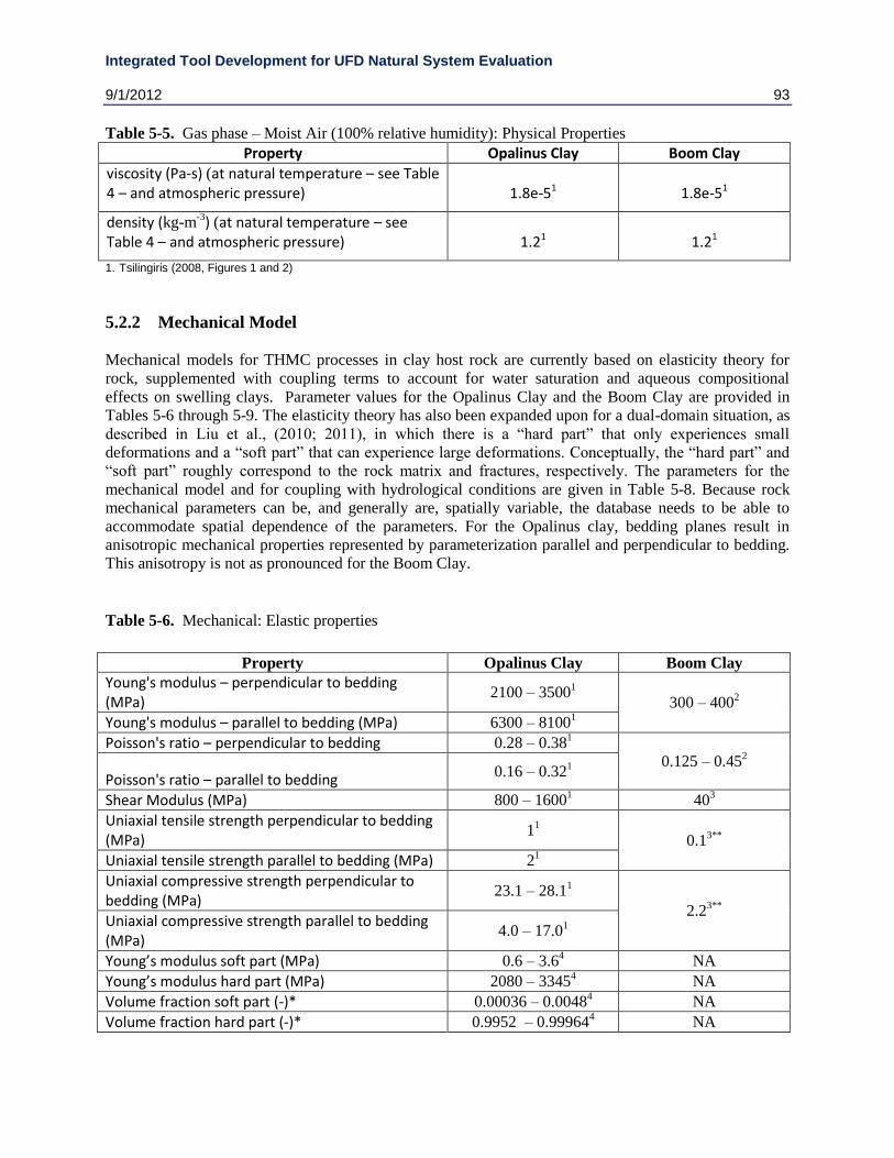
Integrated Tool Development for UFD Natural System Evaluation
9/1/2012 93
Table 5-5. Gas phase – Moist Air (100% relative humidity): Physical Properties
Property Opalinus Clay Boom Clay
viscosity (Pa-s) (at natural temperature – see Table 4 – and atmospheric pressure) 1.8e-51 1.8e-51
density (kg-m-3) (at natural temperature – see
Table 4 – and atmospheric pressure) 1.21 1.21
1. Tsilingiris (2008, Figures 1 and 2)
5.2.2 Mechanical Model
Mechanical models for THMC processes in clay host rock are currently based on elasticity theory for
rock, supplemented with coupling terms to account for water saturation and aqueous compositional
effects on swelling clays. Parameter values for the Opalinus Clay and the Boom Clay are provided in
Tables 5-6 through 5-9. The elasticity theory has also been expanded upon for a dual-domain situation, as
described in Liu et al., (2010; 2011), in which there is a ―hard part‖ that only experiences small
deformations and a ―soft part‖ that can experience large deformations. Conceptually, the ―hard part‖ and
―soft part‖ roughly correspond to the rock matrix and fractures, respectively. The parameters for the
mechanical model and for coupling with hydrological conditions are given in Table 5-8. Because rock
mechanical parameters can be, and generally are, spatially variable, the database needs to be able to
accommodate spatial dependence of the parameters. For the Opalinus clay, bedding planes result in
anisotropic mechanical properties represented by parameterization parallel and perpendicular to bedding.
This anisotropy is not as pronounced for the Boom Clay.
Table 5-6. Mechanical: Elastic properties
Property Opalinus Clay Boom Clay
Young's modulus – perpendicular to bedding (MPa)
2100 – 35001
300 – 4002
Young's modulus – parallel to bedding (MPa) 6300 – 81001
Poisson's ratio – perpendicular to bedding 0.28 – 0.381
0.125 – 0.452
Poisson's ratio – parallel to bedding 0.16 – 0.32
1
Shear Modulus (MPa) 800 – 16001 40
3
Uniaxial tensile strength perpendicular to bedding (MPa)
11
0.13**
Uniaxial tensile strength parallel to bedding (MPa) 21
Uniaxial compressive strength perpendicular to bedding (MPa)
23.1 – 28.11
2.23**
Uniaxial compressive strength parallel to bedding (MPa)
4.0 – 17.01
Young’s modulus soft part (MPa) 0.6 – 3.64 NA
Young’s modulus hard part (MPa) 2080 – 33454 NA
Volume fraction soft part (-)* 0.00036 – 0.00484 NA
Volume fraction hard part (-)* 0.9952 – 0.999644 NA

Integrated Tool Development for UFD Natural System Evaluation
94 9/1/2012
1. Bossart (2012, p. 4-4); 2. Shaw (2010, Table 1); 3. Dehandshutter et al. (2005, Table 1); 4. Liu et al. (2011, Table 2-1); NA = not available
*Note: volume fractions of hard and soft parts add to 1.
** Marked as questionable by Dehandshutter et al. (2005, Table 1).
Table 5-7. Mechanical: Plasticity
Property Opalinus Clay Boom Clay
Plastic limit (%) 21 – 251 22 – 28
2
Liquid limit (%) 33 – 431 59 – 83
2
1. Martin and Lanyon (2003, Table 1); 2. Shaw (2010, Table 1)
Table 5-8. Mechanical: Mohr-Coulomb-Griffith Failure and Moisture Coupling Properties
Property Opalinus Clay Boom Clay
Cohesive strength (MPa) 2.2 – 5.51 0.175 – 0.300
2
Friction angle (°) 24 – 261 18
2
Yield stress (MPa) 20 – 225 NA
Swelling pressure (MPa)* 5.54 0.6
3
Swelling strain (axial, %)* 7.54 5 – 10
3
Swelling strain (radial, %)* 24 NA
Swelling strain (volumetric, %)* 11.54 NA
Swelling pressure perpendicular to bedding (MPa)** 1.21 NA
Swelling pressure parallel to bedding (MPa)** 0.51 NA
Swelling strain perpendicular to bedding (%)** 5 – 91 NA
Swelling strain parallel to bedding (%)** 0.5 – 2.01 NA
1. Bossart (2012, p. 4-21 to 4-23); 2. Dehandshutter et al. (2005, Table 1); 3. Bernier et al. (1997, Figures 14 and 15). 4. Zhang et al. (2010, p. 48-49); 5. Horseman et al. (2005, Figure 20) NA = not available
*Note that the swelling tests reported by Bernier et al. (1997) for the Boom Clay were conducted by controlling relative humidity, which ranged over a complete wetting-drying cycle. Since water was introduced as a vapor, it would also be free of dissolved constituents. Therefore, the swelling data for the Boom Clay represent swelling caused by altering water composition and water content. The swelling data reported by Zhang et al. (2010) for the Opalinus Clay also were measured through controlling capillary pressure through relative humidity and are comparable with those reported by Bernier et al. (1997) for the Boom Clay.
** Note that the swelling tests for the Opalinus Clay reported by Bossart (2012, page 4-23) are conducted using IRSM standard methods. Undisturbed samples that have their native water content are used for the test (Madsen, 1999, page 294). These samples are immersed in distilled water to determine the swelling pressure for confined conditions or swelling strain if unconfined. Because undisturbed samples should be saturated, this test provides information on the effects of changing aqueous composition on swelling stress and strain. It is not clear from the presentation, however, whether swelling strain represents volumetric, axial, or radial strain.

Integrated Tool Development for UFD Natural System Evaluation
9/1/2012 95
Table 5-9. Mechanical: In-Situ Conditions
Property Opalinus Clay Boom Clay
Maximum stress (MPa) 6 – 71 4.5
2
Maximum stress direction (trend, plunge)(°) 210, 701 vertical
Intermediate stress (MPa) 4 – 51 1.4 – 4.1
2
Intermediate stress direction (trend, plunge)(°) 320, 101 horizontal
Minimum stress (MPa) 0.6 – 21 1.4 – 4.1
2
Minimum stress direction (trend, plunge)(°) 50, 151 horizontal
Pore pressure (MPa) 1 – 21 2.2
2
Overconsolidation ratio (OCR) (-) 2.5 – 4.85,6
1 – 2.43,4
1. Martin and Lanyon (2003, p. 1085 and 1087); 2. Bernier et al. (2007, p. 230); 3. Mertens et al. (2003, p. 310) - The minimum OCR for the Boom Clay is an apparent OCR based on the current overburden being the same as the maximum; 4. Shaw (2010, Table 3). 5. Lemy et al. (2006, p. 3) 6. The maximum OCR for the Opalinus Clay is an apparent OCR based on a current overburden of 280 m and a maximum overburden of 1350 m (Bossart, 2012, p. 4-11).
5.2.3 Chemical Model
The current chemical model involves aqueous complexation, cation exchange, and mineral
precipitation/dissolution. Other site-specific information includes aqueous chemical composition, specific
surface areas, and diffusion and sorption parameters. The parameters for chemical processes are given in
Tables 5-10 through 5-17.
Table 5-10. Aqueous: Chemical Composition
Property Opalinus Clay Boom Clay
pH (–log[H+]) 7.3 – 7.961 8.5
2
Eh (mV) -2271 -274
2
Ionic strength (mol-L-1) 0.3501 0.016
2
Mineralization TDS (total dissolved solids) (mg-L-1) 18,2961 935
3
Alkalinity (mEq-L-1) 0.749 –2.51 15.12
2
Total organic carbon (TOC) (mg-L-1 as carbon) 141 150
4
Total inorganic carbon (TIC) (mg-L-1 as carbon) 8.51 181.3
2
pCO2 (log bars) -3.58 to -2.691 -2.62
2
Ca (mg-L-1) 609.01 2.0
2
Li (mg-L-1) 0.41 NA
Na (mg-L-1) 56401 359
2
Mg (mg-L-1) 415.01 1.6
2
K (mg-L-1) 43.41 7.2
2
Fe (mg-L-1) 0.141 0.2
2
Al (mg-L-1) 0.0131 0.6e-3
2
Si (mg-L-1) 1.611 3.4
2
NH4 (mg-L-1) 10.21 NA
Ba (mg-L-1) 0.0191 NA
B (mg-L-1) 1.611 NA

Integrated Tool Development for UFD Natural System Evaluation
96 9/1/2012
Mn (mg-L-1) 0.3461 NA
Sr (mg-L-1) 35.001 NA
Cl (mg-L-1) 10,1701 26
2
SO4 (mg-L-1) 1,3201 2.2
2
Br (mg-L-1) 35.01 0.6
4
HCO3 (mg-L-1) NA 878.92
I (mg-L-1) 2.21 NA
NO3 (mg-L-1) 10.01 NA
NO2 (mg-L-1) 2.01 NA
F (mg-L-1) 0.751 3
4
1. Bossart (2012, p. 4-14 to 4-16); 2. Li et al. (2007, Table 4.2); 3. DeCraen (2006, p. 7); 4. DeCraen et al. (2006, Table 3) NA = not available
A database of thermodynamic parameters that include equilibrium constants, molecular weights of
aqueous species and minerals, parameters for calculating activity coefficients, molar volumes of minerals
is required. A standard database for chemical equilibria is the EQ3/6V7.2b database. This information is
too voluminous to present here, so the general citation to Wolery (1992) is used. This information is site-
specific to the extent that the speciation, compositions, and thermodynamic conditions that are applicable
to the Opalinus Clay and Boom Clay are adequately represented.
Table 5-11. Chemical Reaction: Chemical Equilibrium Parameters
Property Opalinus Clay Boom Clay
Equilibrium constants (dimensions are reaction dependent)
Wolery (1992) Wolery (1992)
Chemical kinetic parameters for a model of the Opalinus Clay are given in Liu et al. (2011, Table 4-7)
and is reproduced here in Table 5-12. Similar parameters should also apply to the Boom Clay, but specific
information for this formation is not available.

Integrated Tool Development for UFD Natural System Evaluation
9/1/2012 97
Table 5-12. Chemical Reaction: Chemical Kinetic Parameters for Opalinus Clay, (Liu et al., 2011, table
4-7)
Mineral
A
(cm2-g
-1)
Parameters for Kinetic Rate Law
Neutral
Mechanism
Acid Mechanism Base Mechanism
k25
(mol-m-2s-1)
Ea
(KJ-
mol-1)
k25
(mol-m-2s-1)
Ea
(KJ-
mol-1)
n(H+) k25
(mol-m-2s-1)
Ea
(KJ-
mol-1)
n(H+)
Primary:
Calcite Assumed at equilibrium
Quartz 9.8 1.02310-14
87.7
K-feldspar 9.8 3.8910-13
38 8.7110-11
51.7 0.5 6.3110-12
94.1 -0.823
Kaolinite 1.95×10⁵ 6.9110
-14 22.2 4.8910
-12 65.9 0.777 8.9110
-18 17.9 -0.472
Illite 6.68×10⁵ 1.6610
-13 35 1.0510
-11 23.6 0.34 3.0210
-17 58.9 -0.4
Chlorite 9.8 3.0210-13
88 7.7610-12
88 0.5
Dolomite 12.9 2.5210-12
62.76 2.3410-7
43.54 1
Ankerite 9.8 1.2610-9
62.76 6.4610-4
36.1 0.5
Smectite-Na 5.64×10⁵ 1.6610
-13 35 1.0510
-11 23.6 0.34 3.0210
-17 58.9 -0.4
Na-montmorillonite 5.64×10⁵ 1.6610
-13 35 1.0510
-11 23.6 0.34 3.0210
-17 58.9 -0.4
Note: k25 = kinetic rate parameter at 25° C, Ea = activation energy, n(H+) = power term (Xu et al., 2006, Table 8)
Additional parameters are needed if transport processes involving dissolved species are to be included in
the model. These parameters relate to diffusion and dispersion phenomena and to sorption interactions
between aqueous species and mineral surfaces. The database needs to be able to accommodate spatial
dependence of these parameters.

Integrated Tool Development for UFD Natural System Evaluation
98 9/1/2012
Table 5-13. Aqueous: Diffusion Coefficient
Property Opalinus Clay Boom Clay
H(HTO) (m2-s-1) parallel to bedding 4e-11 – 1e-101
1.1e-10 – 5.5e-102
H(HTO) (m2-s-1) perpendicular to bedding 1e-11 – 2e-111
H(HTO) accessible porosity (%) 15 – 171 34 – 402
I- (m2-s-1) parallel to bedding 8.0e-12 – 3.0e-111
9.1e-11 – 5.2e-102 I- (m2-s-1) perpendicular to
bedding 2.4e-12 – 4.2e-12 1
I- accessible porosity (%) 5 – 151 14 – 182
Cl- (m2-s-1) parallel to bedding 1.8e-11 – 6.8e-111 NA
Cl- (m2-s-1) perpendicular to bedding 4.8e-121 NA
Cl- accessible porosity (%) 6 – 121 NA
Br- (m2-s-1) parallel to bedding 1.7e-11 – 4.5e-111 NA
Br- accessible porosity (%) 10 – 151 NA
Cs+ (m2-s-1) parallel to bedding 2.6e-10 – 2.7e-101 NA
Cs+ accessible porosity (%) 17 – 181 NA
22Na+ (m2-s-1) parallel to bedding 7.2e-111 NA
22Na+ accessible porosity (%) 17 – 181 NA
85Sr2+(m2-s-1) parallel to bedding 6.5e-11 – 7.0e-111 NA
85Sr2+ accessible porosity (%) 15 – 171 NA
60Co2+ (m2-s-1) parallel to bedding 6.0e-111 NA
60Co2+ accessible porosity (%) 151 NA
6Li+ (m2-s-1) parallel to bedding 7.0e-111 NA
6Li+ accessible porosity (%) 161 NA
SeO42-
(m2-s-1) NA 1.5e-11 – 7.3e-11
3
SeO4 2- accessible porosity (%) NA 5 – 18
3
HSe- (m
2-s-1) NA 8e-11 – 1.7e-103
HSe- accessible porosity (%) NA 12 – 18
3
1. Bossart (2012, p. 4-19 to 4-20); 2. Aertsens et al. (2004, p. 37); 3. De Cannière et al. (2010, Table 5.3-1) NA = not available

Integrated Tool Development for UFD Natural System Evaluation
9/1/2012 99
Table 5-14. Mineralogical: Composition
Property Opalinus Clay Boom Clay
Total clay (% total dry weight) 28 – 931 30 – 60
2
Illite (% total dry weight) 15.0 – 30.01 10 – 45
2
Chlorite (% total dry weight) 3.0 – 18.01 0 – 5
2
Kaolinite (% total dry weight) 15.0 – 37.01 5 – 20
2
Illite/smectite ML (% total dry weight) 5.0 – 20.01 10 – 30
2
Chlorite/smectite ML (% total dry weight) NA 0 – 52
Quartz (% total dry weight) 10.0 – 32.01 15 – 60
2
Feldspars – K (% total dry weight) 0.0 – 6.01 1 – 10
2
Feldspars – albite (% total dry weight) 0.0 – 2.01 1 – 10
2
Calcite (% total dry weight) 4.0 – 22.01 1 – 5
2
Dolomite/ankerite (% total dry weight) 0.0 – 1.01 present
2
Siderite (% total dry weight) 0.0 – 6.01 present
2
Pyrite (% total dry weight) 0.0 – 3.01 1 – 5
2
Gypsum (% total dry weight) 0.0 – 0.51 NA
Organic Carbon (% total dry weight) 0.4 – 1.21 1 – 5
2
1. Bossart (2012, p. 4-12); 2. DeCraen et al. (2004, Table 1-2) NA = not available
Table 5-15. Mineralogical: Cation Exchange Capacity (CEC)
Property Opalinus Clay Boom Clay
Total CEC (mEq/100 g rock) 9.44 – 13.351 24.00
2
Exchangeable Na (mEq/100 g rock) 3.61 – 6.371 8.7
2
Exchangeable K (mEq/100 g rock) 0.58 – 0.921 2.3
2
Exchangeable Ca (mEq/100 g rock) 2.25 – 3.581 3.8
2
Exchangeable Mg (mEq/100 g rock) 1.55 – 2.381 3.7
2
Exchangeable Sr (mEq/100 g rock) 0.10 – 0.361 NA
Selectivity – log(Na/K) 0.7 – 0.843 1.2
2
Selectivity – log(Na/Mg) 0.0 – 2.03 0.32
2
Selectivity – log(Na/Ca) 4.0 to 22.03 0.18
2
Selectivity – log(Na/Sr) 0.0 – 1.03 NA
1. Bossart (2012, p. 4-13); 2. Lolivier et al. (1998, Table II); 3. Pearson et al. (2010, Table 4) NA = not available

Integrated Tool Development for UFD Natural System Evaluation
100 9/1/2012
Table 5-16. Mineralogical: Sorption Coefficients
Property Opalinus Clay * Boom Clay**
H(HTO) (m3-kg-1) 0 - 01 NA
C(inorg.) (m3-kg-1) 0.0016 - 0.00161 NA
C(org.) (m3-kg-1) 0 - 01 NA
Cl(-I) (m3-kg-1) 0 - 01 NA
Ca(II) (m3-kg-1) 0.0002 - 0.00661 NA
Co(II) (m3-kg-1) 0.033 - 7.41 NA
Ni(II) (m3-kg-1) 0.080 - 10.81 NA
Se(-II) (m3-kg-1) 0 - 01 NA
Sr(II) (m3-kg-1) 0.0002 - 0.00661 NA
Zr(IV) (m3-kg-1) 0.56 - 214.01 NA
Nb(V) (m3-kg-1) 0.22 - 72.81 NA
Mo(VI) (m3-kg-1) 0.0011 - 0.2571 NA
Tc(IV) (m3-kg-1) 8.79 - 349.01 52.2 - 65.72
Ru(III/IV) (m3-kg-1) 0.33 - 751 NA
Pd(II) (m3-kg-1) 0.33 - 751 NA
Ag(I) (m3-kg-1) 0 - 01 NA
Cd(II) (m3-kg-1) 0.011 - 2.951 NA
Sn(IV) (m3-kg-1) 7.86 - 15401 NA
Sb(III) (m3-kg-1) 0.22 - 143.01 NA
I(-I) (m3-kg-1) 0 - 0.00051 NA
Cs(I) (m3-kg-1) 0.092 - 3.31 NA
Ce(III) (m3-kg-1) 9.49 - 377.01 NA
Pm(III) (m3-kg-1) 9.49 - 377.01 NA
Sm(III) (m3-kg-1) 9.49 - 377.01 NA
Eu(III) (m3-kg-1) 13.3 - 269.01 0.32 - 12.62
Ho(III) (m3-kg-1) 9.49 - 377.01 NA
Hf(IV) (m3-kg-1) 0.55 - 213.61 NA
Pb(II) (m3-kg-1) 0.057 - 128.01 NA
Po(IV) (m3-kg-1) 0.013 - 2.521 NA
Ra(II) (m3-kg-1) 0.0001 - 0.00461 NA
Ac(III) (m3-kg-1) 2.07 - 139.01 NA
Th(IV) (m3-kg-1) 12.3 - 249.01 0.69 - 21.82
Pa(IV) (m3-kg-1) 0.5 - 501 NA
U(IV) (m3-kg-1) 3.25 - 129.01 NA
Np(IV) (m3-kg-1) 8.79 - 349.01 6.42 - 75.52
Pu(III) (m3-kg-1) 2.76 - 185.01 12.8 - 37.02
Am(III) (m3-kg-1) 2.93 - 98.61 0.86 - 21.82
Cm(III) (m3-kg-1) 2.07 - 139.01 4.87 - 13.42
Pa(V) (m3-kg-1) NA 0.84 - 233.22
Pu(IV) (m3-kg-1) NA 176.9 - 387.02
1. Bradbury and Baeyens (2003, Tables 7 and 9); 2. Maes et al. (2011, p. 1597) NA = not available

Integrated Tool Development for UFD Natural System Evaluation
9/1/2012 101
* Bradbury and Baeyens (2003), Table 7 mean values divided or multiplied by the uncertainty factors in Bradbury and Baeyens (2003) Table 9 **Values computed from retardation factors using conversion given in Maes et al. (2011) Table 4 note a).
Gouy-Chapman theory is used to represent clay swelling effects that result from aqueous compositional
changes (Liu et al., 2011, Section 4). This theory requires density of solid and aqueous phases (Tables 1
and 4), porosity (Table 1), volume fraction of swelling clay minerals (Table 14), exchangeable cations
(Table 15), cation exchange capacity (Table 15), aqueous chemical composition (Table 10), the initial
half-widths between swelling and non-swelling mineral platelets (Table 17), specific surface area (Table
17), and some general scientific parameters such as elementary electric charge and Boltzmann's constant
(Table 18), and the dielectric constant of pore fluid (Table 4).
Table 5-17. Mineralogical: Additional Parameters for the Gouy-Chapman Model Property Opalinus Clay Boom Clay
nondimensional midplane
potential - nondimensional
distance function parameter, a
(for pure smectite) 1.81 – 3.541 1.81 – 3.54
1
nondimensional midplane
potential - nondimensional
distance function parameter, b
(for pure smectite) -4.13 to -3.171 -4.13 to -3.17
1
Basal half-spacing for swelling clay (A) 20 – 40
1 20 – 40
1
Basal half-spacing for non-swelling clay (A) 10
1 10
1
Specific surface area (m2-g-1) 24 – 37 (BET); 112
– 147 (adsorption)2
44 (BET); 200 –
250 (adsorption)3
1. Liu et al. (2011, Table 4-2 and p. 91); 2. Bossart (2012, p. 4-17); 3. Mazurek et al. (2003, p. 160)

Integrated Tool Development for UFD Natural System Evaluation
102 9/1/2012
5.2.4 Thermal Model
The thermal model uses Fourier‘s theory for conductive heat transfer as well as convective heat transfer.
This theory requires thermal conductivity for saturated and dry conditions, the dry bulk rock specific heat,
and aqueous specific heat. Porosity and density of the rock and fractures, as well as the aqueous density
are also needed for the thermal model, but these have already been discussed for the hydrological model.
Thermal-mechanical coupling requires parameters for the thermal expansion of the rock and aqueous
phase. Thermal properties are given in Table 5-18. The database needs to be able to accommodate spatial
dependence of these parameters.
Table 5-18. Thermal: Conductive/Convective Heat Transfer and Thermal-Mechanical
Property Opalinus Clay Boom Clay
bulk rock thermal conductivity parallel to bedding (W-m-1-°C-1) 1.7 – 2.1
1,2
1.35 – 1.73 bulk rock thermal conductivity perpendicular to
bedding (W-m-1-°C-1) 0.8 – 1.2
1,2
bulk rock specific heat (J-kg-1-°C-1) 860 – 9201,2
14024
bulk rock thermal expansion coefficient (°C-1) 1.5e-6 – 1.5e-51,2
1e-5 – 5e-53
aqueous specific heat (J-kg-1-°C-1) (at natural temperature – see Table 4) 4186 – 41885 41855
aqueous thermal conductivity (W-m-1-°C-1) (at natural temperature – see Table 4) 0.595 0.595
aqueous thermal expansion coefficient (°C-1) (at natural temperature – see Table 4) 1.3e-4 – 1.5e-45 1.6e-45
moist air specific heat (J-kg-1-°C-1) (at natural temperature – see Table 4) 1.0e36 1.0e36
moist air thermal conductivity (W-m-1-°C-1) (at natural temperature – see Table 4) 2.5e-26 2.5e-26
thermal expansion coefficient (°C-1) (dry air at 15° C) 3.48e-35 3.48e-35 1. Bossart (2012, p. 4-18); 2. Jobmann and Polster (2007, Table 2); 3. Li et al. (2007, Table 4.4); 4. Li et al. (2007, Tables 4.3 and 4.4 – volumetric heat capacity divided by bulk density) ; 5. Batchelor (1967, Appendix1); 6. Tsilingiris (2008, Figures 3 and 4)

Integrated Tool Development for UFD Natural System Evaluation
9/1/2012 103
5.2.5 Non-Environment-Specific Parameters
Other parameters used for modeling of THMC processes are not environment-specific. These parameters
are summarized in table 5-19.
Table 5-19. Non-Environment-Specific Parameters
Property Value
gravitational acceleration (m-s-2) 9.801
molecular weight (kg) molecule dependent
Boltzmann's constant (J-°C-1) 1.38e-231
elementary electric charge (coulombs (C)) 1.60e-191
permittivity of free space (C2-N-1-m-2) 8.85e-121
1. Reynolds and Perkins (1977, Table A4 and p. 9)
5.3 Data for Modeling Granite Far Field Flow and Transport
Crystalline rock is generally considered a favorable medium that could provide the required safeguard for
long-term storage of nuclear wastes. It may be located in very old, stable tectonic settings. Geochemistry
is often reducing (or can be sited for this), which lowers radionuclide solubilities and increases their
sorption relative to oxidizing environments. Heterogeneity in geochemical/mineralogic properties tends to
be lower than in many other settings. It is very amenable to retrievability (will remain open for very long
periods of time). On the other hand, the hardness of crystalline rock and low matrix porosity and
permeability leads to fracture flow, which tends to be more rapid and less predictable than flow in other
environments. Fracture flow in low porosity environment results in less matrix diffusion and less surface
area available for sorption. Also, it tends to have less sorptive mineralogies than many other rock types.
More reliance is generally needed on engineered barriers for crystalline rock environment because of
these hydrogeologic features. It is expensive to mine, but generally safe and stable. Assessing the
physical, chemical and hydrological properties of crystalline rock is an important step in the investigation
process to identify and select a site with favorable media. Table 5-20 compiles some key granite far field
parameters from different sources.

Integrated Tool Development for UFD Natural System Evaluation
104 9/1/2012
Table 5-20. Sorption Coefficient – SKB1
Data sources: Carbol and Engkvist (1997, SKB technical report R-97-13, table 12-1)
The non-saline and the saline groundwaters are represented by the type of water found at the Gideå and Äspö study
site, respectively. The restrictions for the non-saline water are: pH≥7, [Cl-] < 500 mg/l and Eh< -200 mV. The
restrictions for the saline water are: pH≥7, 500 mg/l < [Cl-] < 6500 mg/l and Eh< -200 mV.
Non-saline Saline
C HCO3 - 0.001 (0.0005-0.002) 0.001 (0.0005-0.002)
Cl Cl 0 - 0 -
Co Co(II) 0.1 (0.05-0.5) 0.02 (0.01-0.1)
Ni Ni(II) 0.1 (0.05-0.5) 0.02 (0.01-0.1)
Se Se(-II, IV,VI) 0.001 (0.0005-0.005) 0.001 (0.0005-0.005)
Kr inert gas 0 - 0 -
Sr Sr(II) 0.01 (0.005-0.05) 0.0002 (0.0001-0.001)
Zr Zr(IV) 1 (0.5-3) 1 (0.5-3)
Nb Nb(V) 1 (0.5-3) 1 (0.5-3)
Tc Tc(IV) 1 (0.3-3) 1 (0.3-3)
Tc Tc(VII) 0 0
Pd Pd(II) 0.1 (0.01-0.5) 0.01 (0.001-0.05)
Ag Ag(I) 0.5 (0.1-1) 0.05 (0.01-0.1)
Cd Cd(II) 0.1 (0.05-0.5) 0.02 (0.01-0.1)
Sn Sn(IV) 0.001 (0-0.01) 0.001 (0-0.01)
I I 0 0 -
Cs Cs(I) 0.5 (0.1-1) 0.05 (0.01-0.1)
Sm Sm(III) 2 (1-5) 2 (1-5)
Eu Eu(III) 2 (1-5) 2 (1-5)
Ho Ho(III) 2 (1-5) 2 (1-5)
Ra Ra(II) 0.1 (0.05-0.5) 0.02 (0.01-0.1)
Ac Ac(III) 3 (1-5) 3 (1-5)
Th Th(IV) 5 (1-10) 5 (1-10)
Pa Pa(IV,V) 1 (0.5-5) 1 (0.5-5)
U U(IV) 5 (1-10) 5 (1-10)
U U(VI) 0.01 (0.005-0.02) 0.005 (0.001-0.01)
Np Np(IV) 5 (1-10) 5 (1-10)
Np Np(V) 0.01 (0.005-0.05) 0.005 (0.001-0.01)
Pu Pu(III,IV) 5 (1-10) 5 (1-10)
Am Am(III) 3 (1-5) 3 (1-5)
Cm Cm(III) 3 (1-5) 3 (1-5)
Uncertainty
intervalElement
Chemical
form/redox state Kd (m3/kg) Kd (m3/kg)
Uncertainty
interval
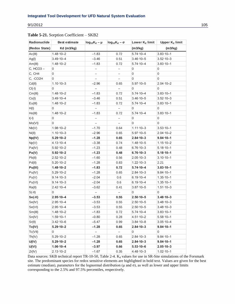
Integrated Tool Development for UFD Natural System Evaluation
9/1/2012 105
Table 5-21. Sorption Coefficient – SKB2
Data sources: SKB technical report TR-10-50, Table 2-4. Kd values for use in SR-Site simulations of the Forsmark
site. The predominant species for redox sensitive elements are highlighted in bold text. Values are given for the best
estimate (median), parameters for the lognormal distribution (μ and σ), as well as lower and upper limits
corresponding to the 2.5% and 97.5% percentiles, respectively.
Radionuclide Best estimate log10Kd – μ log10Kd – σ Lower Kd limit Upper Kd limit
(Redox State) Kd (m3/kg) (m3/kg) (m3/kg)
Ac(III) 1.48·10–2 –1.83 0.72 5.74·10–4 3.83·10–1
Ag(I) 3.49·10–4 –3.46 0.51 3.46·10–5 3.52·10–3
Am(III) 1.48·10–2 –1.83 0.72 5.74·10–4 3.83·10–1
C, HCO3 – 0 – – 0 0
C, CH4 0 – – 0 0
C, -CO2H 0 – – 0 0
Cd(II) 1.10·10–3 –2.96 0.65 5.97·10–5 2.04·10–2
Cl(-I) 0 – – 0 0
Cm(III) 1.48·10–2 –1.83 0.72 5.74·10–4 3.83·10–1
Cs(I) 3.49·10–4 –3.46 0.51 3.46·10–5 3.52·10–3
Eu(III) 1.48·10–2 –1.83 0.72 5.74·10–4 3.83·10–1
H(I) 0 – – 0 0
Ho(III) 1.48·10–2 –1.83 0.72 5.74·10–4 3.83·10–1
I(-I) 0 – – 0 0
Mo(VI) 0 – – 0 0
Nb(V) 1.98·10–2 –1.70 0.64 1.11·10–3 3.53·10–1
Ni(II) 1.10·10–3 –2.96 0.65 5.97·10–5 2.04·10–2
Np(IV) 5.29·10–2 –1.28 0.65 2.84·10–3 9.84·10–1
Np(V) 4.13·10–4 –3.38 0.74 1.48·10–5 1.15·10–2
Pa(IV) 5.92·10–2 –1.23 0.48 6.76·10–3 5.18·10–1
Pa(V) 5.92·10–2 –1.23 0.48 6.76·10–3 5.18·10–1
Pb(II) 2.52·10–2 –1.60 0.56 2.05·10–3 3.10·10–1
Pd(II) 5.20·10–2 –1.28 0.83 1.22·10–3 2.21
Pu(III) 1.48·10–2 –1.83 0.72 5.74·10–4 3.83·10–1
Pu(IV) 5.29·10–2 –1.28 0.65 2.84·10–3 9.84·10–1
Pu(V) 9.14·10–3 –2.04 0.6 6.19·10–4 1.35·10–1
Pu(VI) 9.14·10–3 –2.04 0.6 6.19·10–4 1.35·10–1
Ra(II) 2.42·10–4 –3.62 0.41 3.87·10–5 1.51·10–3
S(-II) 0 – – 0 0
Se(-II) 2.95·10–4 –3.53 0.55 2.50·10–5 3.48·10–3
Se(IV) 2.95·10–4 –3.53 0.55 2.50·10–5 3.48·10–3
Se(VI) 2.95·10–4 –3.53 0.55 2.50·10–5 3.48·10–3
Sm(III) 1.48·10–2 –1.83 0.72 5.74·10–4 3.83·10–1
Sn(IV) 1.59·10–1 –0.80 0.28 4.51·10–2 5.58·10–1
Sr(II) 3.42·10–6 –5.47 0.99 3.84·10–8 3.05·10–4
Tc(IV) 5.29·10–2 –1.28 0.65 2.84·10–3 9.84·10–1
Tc(VII) 0 – – 0 0
Th(IV) 5.29·10–2 –1.28 0.65 2.84·10–3 9.84·10–1
U(IV) 5.29·10–2 –1.28 0.65 2.84·10–3 9.84·10–1
U(VI) 1.06·10–4 –3.97 0.66 5.53·10–6 2.05·10–3
Zr(IV) 2.13·10–2 –1.67 0.35 4.48·10–3 1.02·10–1

Integrated Tool Development for UFD Natural System Evaluation
106 9/1/2012
Table 5-22. Sorption Coefficient – JAEA
Note: Data with de-ionized and other water chemistry that are obviously not relevant are not included except for Ac
and Pd. For these two species no other data are available.
Data sources: Japan JAEA database: http://migrationdb.jaea.go.jp/english.html
Table 5-23. Sorption Coefficient – SNL
Data sources: Mariner et al. (2011), table 2-3.
Data (range) Geometric mean Geometric STDV Mean of log10(data)
(unit: cc/g) (cc/g) (dimensionless) data unit (m3/kg)
Am 220 - 190000 9096.03 4.306 0.959 0.634
Pu 0.2 - 401000 1736.9 13.957 0.24 1.145
Np 0.65 - 2720 31.61 5.667 -1.5 0.753
U 0 - 280000 16.04 9.215 -1.795 0.965
Tc 0.1 - 200000 15.5 56.54 -1.81 1.752
Sn 173 - 2940 688.4 2.754 -0.162 0.44
Cs 1 - 131000 135.76 7.991 -0.867 0.903
I 0.5 – 1.9 0.89 1.43 -3.052 0.155
Se 0 - 18 2.63 3.114 -2.579 0.493
Th 501 - 10000 1245.51 2.322 0.095 0.366
Pa 2.4 – 7.3 4.14 1.558 -2.383 0.193
Ra 30.1 - 3800 504.84 4.302 -0.297 0.634
Pb 1600 - 4400 2653.3 1.658 0.424 0.22
Sr 1 - 880 20.87 3.785 -1.68 0.578
Sb 450 - 519 483.27 1.074 -0.316 0.031
Zr 2.6 - 3160000 839.02 12.746 -0.076 1.105
Nb 7 - 142000 465.596 4.996 -0.332 0.699
Ac 83 - 40000 6687.15 8.17 0.825 0.912
Pd 142 - 82800 2256.63 5.301 0.353 0.724
Species STDV of log10(data)
Element Kd (m3/kg)
C, Cl, I 0
Se 0.0005
Pd, Sn 0.001
Sr 0.005
Nb 0.02
Am, Cm, Ac 0.04
Pa, Tc, Cs 0.05
Sb 0.1
U 0.1
Np, Th, Ra, Zr 0.2
Pu 0.5
Pb 1

Integrated Tool Development for UFD Natural System Evaluation
9/1/2012 107
Table 5-24. Solubility – SNL
Element Solubility Units
Actinium (Ac) 6.00E-06 mol/L
Americium (Am) 6.00E-06 mol/L
Carbon (C ) 1.00E+50 mol/L
Curium (Cm) 6.00E-06 mol/L
Cesium (Cs) 1.00E+50 mol/L
Iodine (I) 1.00E+50 mol/L
Niobium (Nb) 4.00E-05 mol/L
Neptunium (Np) 1.00E-09 mol/L
Protactinium (Pa) 1.00E-09 mol/L
Lead (Pb) 1.00E+50 mol/L
Paladium (Pd) 3.00E-06 mol/L
Plutonium (Pu) 2.00E-07 mol/L
Radium (Ra) 1.00E-06 mol/L
Antimony (Sb) 1.00E-07 mol/L
Selenium (Se) 4.00E-08 mol/L
Tin (Sn) 3.00E-08 mol/L
Strontium (Sr) 1.00E+50 mol/L
Technetium (Tc) 3.00E-08 mol/L
Thorium (Th) 4.00E-07 mol/L
Uranium (U) 4.00E-10 mol/L
Zirconium (Zr) 2.00E-08 mol/L Note: no limit represented by 1E+50 mol/L
Data sources: Mariner et al. (2011), table 2-5 (pH 7.5, T = 25 deg C).
C, Cs, I, Sr, and Pb assumed infinitely soluble.

Integrated Tool Development for UFD Natural System Evaluation
108 9/1/2012
Table 5-25. Solubility – SKB
Data sources: SKB technical report TR-10-50, Table 3-4, for temperate condition.
Note: 1.x1017
represents unlimited solubility.
Element Solubility Unit
Ac-227 1.00·1017 mol/L
Ag-108m 1.10·10–5 mol/L
Am-241 2.50·10–6 mol/L
Am-242m 2.50·10–6 mol/L
Am-243 2.50·10–6 mol/L
C-14 1.00·1017 mol/L
Cd-113m 1.00·1017 mol/L
Cl-36 1.00·1017 mol/L
Cm-245 2.60·10–6 mol/L
Cm-246 2.60·10–6 mol/L
Cs-135 1.00·1017 mol/L
Cs-137 1.00·1017 mol/L
Eu-152 1.00·1017 mol/L
H-3 1.00·1017 mol/L
Ho-166m 4.10·10–6 mol/L
I-129 1.00·1017 mol/L
Mo-93 1.00·1017 mol/L
Nb-93m 4.90·10–5 mol/L
Nb-94 4.90·10–5 mol/L
Ni-59 3.00·10–4 mol/L
Ni-63 3.00·10–4 mol/L
Np-237 1.00·10–9 mol/L
Pa-231 3.30·10–7 mol/L
Pb-210 1.70·10–6 mol/L
Pd-107 3.90·10–6 mol/L
Pu-238 4.80·10–6 mol/L
Pu-239 4.80·10–6 mol/L
Pu-240 4.80·10–6 mol/L
Pu-242 4.80·10–6 mol/L
Ra-226 9.10·10–7 mol/L
Se-79 6.70·10–9 mol/L
Sm-151 1.10·10–7 mol/L
Sn-121m 9.00·10–8 mol/L
Sn-126 9.00·10–8 mol/L
Sr-90 3.70·10–3 mol/L
Tc-99 3.80·10–9 mol/L
Th-229 2.60·10–9 mol/L
Th-230 2.60·10–9 mol/L
Th-232 2.60·10–9 mol/L
U-233 9.50·10–10 mol/L
U-234 9.50·10–10 mol/L
U-235 9.50·10–10 mol/L
U-236 9.50·10–10 mol/L
U-238 9.50·10–10 mol/L
Zr-93 1.80·10–8 mol/L

Integrated Tool Development for UFD Natural System Evaluation
9/1/2012 109
Table 5-26. Diffusivity - JAEA
Note: Dp (pore diffusivity) (Dp = De/porosity) is generally used in dual-porosity model as matrix diffusion
coefficient. Data with de-ionized water are not included. Blank line means no data available.
Data sources: Japan JAEA database: http://migrationdb.jaea.go.jp/english.html
De : effective
diffusivity (range)
Dp : pore
diffusivity
(range)
(unit: m2/s) (unit: m
2/s)
Am
Pu 1.28e-13 – 2.76e-13 2.61e-11 – 5.63e-11 4.10E-11 1.07E-11
Np 2.10e-13 – 5.41e-13 2.80e-11 – 1.10e-10 6.99E-11 2.75E-11
U 2.20e-14 – 4.40e-14 3.14e-12 – 6.29e-12 5.14E-12 1.42E-12
Tc 4.20e-14– 4.20e-14 4.20e-12 – 4.20e-12 4.20E-12 0
Sn
Cs 5.04e-13– 1.80e-11 1.03e-10– 3.75e-10 2.11E-10 1.05E-10
I 3.90e-13– 2.60e-12 7.96e-11– 3.38e-10 1.57E-10 6.02E-10
Se 1.90e-12– 5.30e-12 8.26e-11– 9.46e-11 8.93E-11 5.00E-12
Th
Pa
Ra
Pb
Sr 2.00e-13– 1.60e-12 2.86e-11– 4.00e-10 6.65E-11 9.66E-11
Sb
Zr
Nb
Ac
Pd
Species Mean (Dp)Standard
Deviation (Dp)

Integrated Tool Development for UFD Natural System Evaluation
110 9/1/2012
Table 5-27. Various Far Field Parameters
SKB technical report TR-10-52, table 6-91
Data sources:
1. SKB technical report TR-10-52, Table 3-2
2. SKB technical report TR-10-52, Table 3-2
3. Sandia report SAND2011-6203, p75-76
4. SKB technical report TR-10-52, Table 6-85
5. SKB technical report TR-10-50, Table 3-5
6. SKB technical report TR-10-50
7. SKB technical report TR-10-50
8. SKB technical report TR-10-52, Table 6-78
9. Sandia report SAND2011-6203, Table 1-3
10. Posiva 2010. Models and Data Report 2010. POSIVA 2010-01. Posiva Oy, Olkiluoto, Finland.
11. Kalinina et al. Paper "Analysis of the Effect of Hterogeneity on Heat Extraction in an EGS Represented
with the Continuum Fracture Model", data from granite sites in US, Czech Republic, France, Spain,
Portugal, Sweden, Egypt and Japan.
12. Kalinina et al. Paper "Analysis of the Effect of Hterogeneity on Heat Extraction in an EGS Represented
with the Continuum Fracture Model", data from granite sites in US, Czech Republic, France, Spain,
Portugal, Sweden, Egypt and Japan.
13. Kalinina et al. Paper "Analysis of the Effect of Hterogeneity on Heat Extraction in an EGS Represented
with the Continuum Fracture Model", data from granite sites in US, Czech Republic, France, Spain,
Portugal, Sweden, Egypt and Japan.
14. based on values at Forsmark and Laxemar (SKB 2006, Table 9-4)
15. based on values at Forsmark and Laxemar (SKB 2006, Table 9-4)
16. SKB technical report TR-10-52, Table 6-91
17. SKB technical report TR-10-52, Table 6-91
Parameter Description Value mean Stdv UnitsDistribution
TypeIndex
Bulk Density 2700 kg/m3 1
Porosity 0.0018 [] 2
permeasbility 10-20 to 10-19 m2 3
Longitude dispersivity 50 m 4
Equivalent flow rate 4.2x10⁻⁶ to 1.2x10⁻⁴ m3/yr 5
Colloid concentrations 10 mg/l 6
Colloid concentrations (with dilute glacial melt water)10
g/l 7
Hydraulic conductivity (for depth 200 to 400 m) 3x10⁻⁹ to 1x10⁻⁷ m/s 8
Hydraulic conductivity (for depth > 400 m) 10-13 to 10-10 m/s 9
Fracture zone mean fracture aperture 5x10⁻⁴ m 10
Fracture aperture 10-5 to 3x10⁻³ m 11
Fractutre spacing 0.25 to 15 m 12
Fracture length 1.5 to 76 m 13
Heat conductivity 2.77 to 3.34 W m-1 K-1 14
Heat capacity 2.17 to 2.24 MJ m-3 K-1 15
Best estimate Log10De (m2/s) Log10De (m2/s)
Effective diffusivity (cations, non-charged solutes) 2.1x10⁻¹⁴ -13.7 0.25 m2/s Log-normal 16
Effective diffusivity (anions) 6.6x10⁻¹⁵ -14.2 0.25 m2/s Log-normal 17

Integrated Tool Development for UFD Natural System Evaluation
9/1/2012 111
Table 5-28. Global Transport Parameter
Note: 500 m travel distance. Should be scaled to other values.
Data sources: SKB technical report TR-10-52, Figure 6-67; Painter, S., Cvetkovic, V., Mancillas, J., Pensado, O.
(2008): Time domain particle tracking methods for simulating transport with retention and first-order
transformation. Water Resources Research 43(9), W01406; SKB. 2010. Radionuclide transport report for the safety
assessment SR-Site. SKB Technical Report TR-10-50. Swedish Nuclear Fuel and Waste Management Co.
The parameters hydrodynamic transport resistance and global travel time are integrated quantities of a
flowpath/streamline. Within some models of radionuclide transport (e.g. Painter et al., 2008 and SKB, 2010), these
two parameters are the only flow related parameters controlling radionuclide transport. The transport resistance
parameter is the flow-rate normalized flow-wetted surface area of a streamtube of infinitesimal cross-section. It is
denoted beta in Painter et al. (2010) and F in SKB (2010). The global travel time is the travel time of a non-
dispersing, non-sorbing, non-diffusing tracer moving with the groundwater flow.
Median 5 percentilce 95 percentile Unit
Hydrodynamic Transport Resistance Parameter (F) 4.00E+06 3.00E+05 1.00E+08 yr/m
Travel time 150 30 1000 yr

Integrated Tool Development for UFD Natural System Evaluation
112 9/1/2012
Table 5-29. Groundwater Composition
Note: nr =not reported
Data sources: Mariner et al. (2011), table 2-1 Sample groundwater composition in granite at depths from 360 to 708
m.
ParameterOlkiluoto,
Finland
Olkiluoto,
Finland
Olkiluoto,
Finland
Laxemar,
Sweden
Forsmark,
Sweden
Pinawa,
Canada
East Bull
Lake,
Canada
Borehole OL-KR20 OL-KR10 OL-KR12 KLX03 KFM02A WN-4 EBL-2
Depth (m) 360 487 708 380 512 513 538
TDS (g L-1
) 10.5 22.1 49.5 2.8 9.3 7.5 2.3
Ionic strength
(eq L-1
) 0.22 0.48 1.18 0.05 0.19 0.16 0.05
pH 7.4 8 8.2 7.9 7.2 8.1 7.4
Na (mol L-1
) 0.11 0.21 0.36 0.03 0.09 0.07 0.03
Ca (mol L-1
) 0.03 0.09 0.25 0.01 0.02 0.03 0.01
K (mol L-1
) 2.8E-04 3.6E-04 4.9E-04 1.4E-04 9.0E-04 5.3E-04 5.4E-05
Mg (mol L-1
) 2.6E-03 1.6E-03 1.5E-03 4.4E-04 9.3E-03 1.1E-03 7.0E-05
Sr (mol L-1
) 1.6E-04 3.7E-04 1.1E-03 nr nr nr 3.3E-05
Mn (mol L-1
) 5.8E-06 7.3E-06 9.3E-06 nr nr nr nr
Cl (mol L-1
) 0.18 0.38 0.86 0.04 0.15 0.11 0.04
SO4 (mol L-1
) 2.1E-04 1.0E-05 5.0E-05 1.3E-03 5.2E-03 6.6E-03 1.4E-04
CO3 (mol L-1
) 5.5E-04 1.1E-04 4.0E-05 3.1E-03 2.2E-03 3.5E-03 5.0E-04
SiO2 (mol L-1
) 3.6E-04 2.8E-04 2.1E-04 nr nr nr 5.4E-05
Fe (mol L-1
) 2.5E-06 2.0E-06 3.8E-07 8.0E-06 3.3E-05 nr nr
S(-II) (mol L-1
) 5.6E-06 <3.1 E-7 1.3E-06 3.0E-07 0.0E+00 nr nr
Reference Posiva (2010),
Table 6-6
Posiva (2010),
Table 6-6
Posiva (2010),
Table 6-6
SKB (2006d), p.
382
SKB (2006d),
p. 382
Gascoyne et
al. (1987),
Table 3
Gascoyne et
al. (1987),
Table 3

Integrated Tool Development for UFD Natural System Evaluation
9/1/2012 113
Table 5-30. Groundwater chemistry information for granite in Japan
*DIC=Dissolved Inorganic Carbon=HCO3- + CO32-
Data sources: T. Iwatsuki et al., Applied Geochemistry 20 (2005) 2283-2302.
Analyte Unit Results (range)
Temperature 0C 17.5 - 25
pH 8.1 – 9.2
Eh mv 0 - -280
Conductivity ms/m 32.7 - 525
Na+ mg/L 58.7 – 393.5
K+ mg/L 0.2 – 9.4
Ca2+ mg/L 5.9 – 638.6
Ma2+ mg/L <0.1 – 0.4
Si mg/L 5.5 – 8.6
DIC* mg/L 0 – 12.3
SO32- mg/L <0.4 – 9.5
Cl- mg/L 37.5 – 1645.4
F- mg/L 1.7 – 12.0
Br- mg/L <0.1 – 2.9

Integrated Tool Development for UFD Natural System Evaluation
114 9/1/2012
Figure 5-1. Major ion chemistry of Canadian granite water (values are total dissolved solids) (Gascoyne,
2004)

Integrated Tool Development for UFD Natural System Evaluation
9/1/2012 115
Figure 5-2. Major ions of Canadian granite water as a function of depth below surface in meters (mg/L)
(Gascoyne, 2004). pH values (7 to 9) with no obvious trend with depth, while Eh values (-200 to 300)
with tendency toward lower (more reducing) values with increasing depth.

Integrated Tool Development for UFD Natural System Evaluation
116 9/1/2012
Figure 5-3. Chloride distribution with depth for Swedish granite sites (Laaksoharju et al., 2008):
Laxemar (green), Simpevarp (red), Forsmark (blue). Open symbols represent samples considered
unsuitable. Elevation indicated above sea level. Note: Chloride charge is balanced almost entirely by
Na+ and Ca
2+ (the sum of the concentrations of these two ions should be approximately 4/7
ths that of Cl
- in
mg/L).
Figure 5-4. Eh and pH ranges at Swedish sites (Eh generally decreases with depth) (Laaksoharju et al.,
2008).

Integrated Tool Development for UFD Natural System Evaluation
9/1/2012 117
Forsmark site.
Laxemar/Simpevarp site
Figure 5-4. Types and distributions of groundwater at two Swedish granite sites (Laaksoharju et al.,
2008). A - fresh groundwater (<2000 mg/L Cl; 0.5–3.5 g/L TDS), mainly meteoric and Na–HCO3 in
type, and marginally oxidizing close to the surface, otherwise reducing. BL - brackish groundwater (2000–
10,000 mg/L Cl; 3.5–18.5 g/L TDS), meteoric, mainly Na–Ca–Cl in type, glacial/deep saline components,
and reducing; BS - brackish groundwater (2000–10,000 mg/L Cl, 3.5–18.5 g/L TDS). meteoric, mainly
Na–Ca–Cl in type but some Na–Ca(Mg)–Cl(Br) types, glacial/deep saline components, and reducing; C -
saline (10,000–20,000 mg/L Cl; 18.5–30 g/L TDS), dominantly Ca–Na–Cl in type at Laxemar but Na–
Ca–Cl changing to Ca–Na–Cl only at the highest salinity levels at the Simpevarp site, and reducing; and
D - highly saline (>20,000 mg/L Cl; to a maximum of ~70 g/L TDS), dominantly Ca–Na–Cl, and
reducing.

Integrated Tool Development for UFD Natural System Evaluation
118 9/1/2012
Table 5-31. Groundwater chemistry of Switzerland Grimsel test site (~1730 m above sea level) (Schafer
and Iijima, 2007). Low ionic strength water (~0.001 M, ~50 mg/L TDS), dominated by NaHCO3
(secondary ions are Ca2+
and Cl-) with Eh = -200 ± 50 mV and pH = 9.5 ± 0.2.
Parameter Value Unit
pH 9.6
Eh -170 mV
Ionic
Strength0.0017 M
Na 0.56 mM
K 0.006 mM
Mg 0.00058 mM
Ca 0.14 mM
Al 12.7 ppb
SO42- 0.052 mM
F- 0.31 mM
Cl- 0.15 mM
HCO3- 0.283 mM

Integrated Tool Development for UFD Natural System Evaluation
9/1/2012 119
Table 5-31. Formation Properties
aApproximate range of flow porosities, which are 1/10th the approximate diffusion porosities (Posiva, 2010, tables
C-3, C-4, and C-5); Mariner et al. (2011).
Porosity
(m s-1) (GPa) (MPa)
Barre Granite,
Vermont
Krech et al.
(1974) Granodiorite 0.51 < 10-10 46 0.23 197
St. Cloud
Granodiorite,
Minnesota
Krech et al.
(1974) Granodiorite 0.08 < 10-10 71 0.25 282
Westerly
Granite, Rhode
Island
Krech et al.
(1974) Granodiorite 0.35 < 10-10 50 0.21 233
10-12 – 10-5 (<400 m)
10-13 – 10-10 (>400 m)
10-7 (near surface)
10-11 (at depth)
10-10 – 10-5 (<200 m)
10-11 – 10-6 (>200 m)
Location Reference Lithologic
Classification
Sherman
Granite,
Wyoming
Touloukian et
al. (1981) Granite 0.002 9.8 × 10⁻¹³
Granite,
Wyoming
Touloukian et
al. (1981) Granite
Fremont
Canyon
Touloukian et
al. (1981) Granite 45
California Touloukian et
al. (1981) Granodiorite
Stone Mountain
Granite,
Georgia
Touloukian et
al. (1981);
Hoek & Brown
(1980)
Granite 0.3
Hardhat Granite Touloukian et
al. (1981) Granite 4 × 10-14
Olkiluoto,
Finland Posiva (2010)a Pegmatitic
granite 0.01 – 0.2 65
0.09
Atikokan,
Ontario
Gascoyne et
al. (1987) Granite
76
Bulk Hydraulic
Conductivity
(%)
Young’s
ModulusPoisson’s Ratio
Compressive
Strength
Laxemar,
Sweden
SKB (2006b),
Table A-42;
SKB (2006d)
Granite to
Granodiorite 0.14
Forsmark,
Sweden
SKB (2006b),
Table A-42
Granite to
Granodiorite 0.24
116
0.29 108
165-210
142, 129
0.1
116

Integrated Tool Development for UFD Natural System Evaluation
120 9/1/2012
5.4 References
Aertsens, M., Put, M., and Dierckx, A. (2003) An Analytical Model for the Interpretation of Pulse
Injection Experiments Performed for Testing the Spatial Variability of Clay Formations, Journal
of Contaminant Hydrology 61 (2003) 423– 436.
Aertsens, M., Wemaere, I., Wouters, L. (2004) Spatial variability of Transport Parameters in the Boom
Clay, Applied Clay Science, 26, 37– 45.
Arnould, M. (2006) Discontinuity Networks in Mudstones: A Geological Approach - Implications for
Radioactive Wastes Isolation in Deep Geological Formations in Belgium, France, Switzerland,
Bull Eng Geol Environ (2006) 65:413–422.
Batchelor, G.K. (1967) An Introduction to Fluid Dynamics, Cambridge University Press.
Bernier, F., Li, X.-L., And Bastiaens, W. (2007) Twenty-Five Years‘ Geotechnical Observation and
Testing in the Tertiary Boom Clay Formation, Géotechnique, 57, No. 2, 229–237.
Bernier, F., Volckaert, G., Alonso, E., Villar, M. (1997) Suction-Controlled Experiments on Boom Clay,
Engineering Geology, 47, 325-338.
Bernier, F., and B. Neerdael. (1996) Overview of In-Situ Thermomechanical Experiments in Clay:
Concept, Results and Interpretation, Engineering Geology, 41, 51-64.
Bertrand, F., L. Laloui, C. Laurent. (2009) Thermo-Hydro-Mechanical Simulation of ATLAS In Situ
Large Scale Test in Boom Clay, Computers and Geotechnics, 36, 626–640.
Bossart, P. (2012) Characteristics of the Opalinus Clay at Mont Terri. http://www.mont-
terri.ch/internet/mont-
terri/en/home/geology/key_characteristics.parsys.49924.DownloadFile.tmp/characteristicsofopa.p
df
Bossart, P., Trick, T., Meier P.M., Mayord, J.-C. (2004) Structural and Hydrogeological Characterisation
of the Excavation-Disturbed zone in the Opalinus Clay (Mont Terri Project, Switzerland),
Applied Clay Science, 26, 429– 448.
Bradbury, M., and Baeyens, B. (2003) Far Field Sorption Data Bases for Performance Assessment of a
High-Level Radioactive Waste Repository in an Undisturbed Opalinus Clay Host Rock, Nuclear
Energy and Safety Research Department Laboratory for Waste Management, PSI Bericht Nr. 03-
08, Nagra NTB 02-19, http://les.web.psi.ch/publications/Liste03.html
Carbol, P. and Engkvist, I. (1997) Compilation of radionuclide sorption coefficients for performance
assessment, SKB rapport R-97-13.
Cosgrove, J.W. (2001) Hydraulic Fracturing During the Formation and Deformation of a Basin: A Factor
in the Dewatering of Low-Permeability Sediments, AAPG Bulletin, v. 85, no. 4, pp. 737–748.
De Cannière, P., Maes, A., Williams, S., Bruggeman, C., Beauwens, T., Maes, N., and Cowper, M.
(2010) Behaviour of Selenium in Boom Clay, External Report, SCK•CEN-ER-120, 10/PDC/P-9.
http://publications.sckcen.be/dspace/bitstream/10038/7079/1/er_120.pdf

Integrated Tool Development for UFD Natural System Evaluation
9/1/2012 121
De Craen, M. (2006) The Boom Clay Geochemistry: Natural Evidence, Mat. Res. Soc. Symp. Proc. Vol.
932 © 2006 Materials Research Society.
De Craen, M., Wemaere, I., Labat, S., and Van Geet, M. (2006) Geochemical analyses of Boom Clay
Pore Water and Underlying Aquifers in the Essen-1 Borehole, External Report of the Belgian
Nuclear Research Centre, SCK•CEN-ER-19, 06/MDC/P-47.
http://publications.sckcen.be/dspace/bitstream/10038/430/1/er_19.pdf
De Craen, M., Wang, L., Van Geet M., and Moors, H. (2004) Geochemistry of Boom Clay Pore Water at
the Mol Site, Scientific Report, SCK•CEN-BLG-990, 04/MDC/P-48.
http://www.google.com/url?sa=t&rct=j&q=&esrc=s&frm=1&source=web&cd=3&ved=0CDkQF
jAC&url=http%3A%2F%2Fwww.sckcen.be%2Ffr%2Fcontent%2Fdownload%2F16123%2F217
784%2Fversion%2F1%2Ffile%2FGeochemistry%2Bof%2BBoom%2BClay%2Bpore%2B-
%2BStatus%2B2004.pdf&ei=Db-
ET9f4DImPiALfsvD1BA&usg=AFQjCNHOtkH7XpWt0uWNceqVyWex0po6nQ
Degueldre, C., Andreas Scholtis, A., Laube, A.,Turrero, M.J., and Thomas, B. (2003) Study of the Pore
Water Chemistry through an Argillaceous Formation: A Paleohydrochemical Approach, Applied
Geochemistry, 18, 55–73.
Dehandschutter, B., Vandycke, S., Sintubin, M., Vandenberghe, N., Wouters, L. (2005) Brittle Fractures
and Ductile Shear Bands in Argillaceous Sediments: Inferences from Oligocene Boom Clay
(Belgium), Journal of Structural Geology 27 (2005) 1095–1112.
De Windt, L., Pellegrini, D., and van der Lee, J. (2004) Reactive Transport Modelling of a Spent Fuel
Repository in a Stiff Clay Formation Considering Excavation Damaged Zones, Radiochim. Acta
92, 841–848.
Dymitrowska, M., Genty, A., Lukin, D., Navarro, D., Weetjens, E. (2009) PAMINA-Performance
Assessment Methodologies in Application to Guide Development of the Safety Case – PA
Approach to Gas Migration, Deliverable D-No :3.2.1, European Commission under the Euratom
Research and Training Programme on Nuclear Energy within the Sixth Framework Programme
(2002-2006). http://www.ip-pamina.eu/downloads/pamina3.2.1.pdf
Fischer, H.B., List, E.J., Koh, R.C.Y., Imberger, J., Brooks, N.H. (1979) Mixing in Inland and Coastal
Waters, Academic Press.
Gascoyne, M. (2004) Hydrogeochemistry, groundwater ages and sources of salts in a granitic batholith on
the Canadian Shield, Southeastern Manitoba, Applied Geochemistry, 19, 519-560.
Horseman, S.T., Harrington, J.F., Birchall, D.J., Noy, D.J., and Cuss, R.J. (2005) Consolidation and
Rebound Properties of Opalinus Clay: A Long-Term, Fully-Drained Test, Environmental
Protection Programme Commissioned Report CR/05/128N, Technical Report CR/05/128, British
Geological Survey. http://nora.nerc.ac.uk/11314/1/CR05128N.pdf
Iwatsuki, T., Furue, R., Mie, H., Ioka, S. and Mizuno, T. (2005) Hydrochemical baseline condition of
groundwater at the Mizunami underground research laboratory (MIU), Applied Geochemistry, 20,
2283-2302.

Integrated Tool Development for UFD Natural System Evaluation
122 9/1/2012
JAEA (Japan Atomic Energy Agency) Diffusion and sorption coefficient database. Japan Atomic Energy
Agency. http://migrationdb.jaea.go.jp/english.html.
Jobmann, M., and Polster, M. (2007) The Response of Opalinus Clay Due to Heating: A Combined
Analysis of In Situ Measurements, Laboratory Investigations and Numerical Calculations,
Physics and Chemistry of the Earth, 32, 929–936.
Johnson, L., Marschall, P., Zuidema, P., Gribi, P. (2004) Effect of Post-Disposal Gas Generation in a
Repository for Spent Fuel, High-Level Waste, and Long-Lived Intermediate-Level Waste Sited in
Opalinus Clay, Nagra Technical Report 04-06.
http://www.nagra.ch/documents/database/dokumente/$default/Default%20Folder/Publikationen/
NTBs%202001-2010/e_ntb04-06.pdf
Kalinina, E., McKenna, S.A., Hadgu, T. and Lowry, T. (2012) Analysis of the Effect of Heterogeneity on
heat extraction in an EGS represented with the continuum fracture model, Proceedings of 37th
Stanford Geothermal Reservoir Engineering Workshop, January 30 – February 1, 2012, Stanford,
California.
Klein, L.A., Swift, C.T. (1977) An Improved Model for the Dielectric Constant of Sea Water at
Microwave Frequencies, IEEE Transactions on Antennas and Propagation.
Laaksoharju, M., Smellie, J., Tullborg, E., Gimeno, M., Molinero, J., Gurban, I. and Hallbeck, L. (2008)
Hydrogeochemical evaluation and modelling performed within the Swedish site investigation
programme, Applied Geochemistry, 23, 1761-1795.
Lemy, F., Yong, S., And Schulz, T. (2006) A Case Study of Monitoring Tunnel Wall Displacement using
Laser Scanning Technology, IAEG2006 Paper number 482, The Geological Society of London
2006.
Li, X., Bernier, F., Vietor, T., Lebon, P. (2007) TIMODAZ (Contract Number: FI6W-CT-036449),
DELIVERABLE ( N°: 2), European Commission Community Research.
http://www.google.com/url?sa=t&rct=j&q=&esrc=s&frm=1&source=web&cd=1&sqi=2&ved=0
CCAQFjAA&url=http%3A%2F%2Fwww.timodaz.eu%2Fdeliverables.aspx%3Fdwnld%3DTIM
ODAZD2formatECfinal.doc%26itemid%3Dbc9c5d91-17e1-4cec-929c-
2c8a49ff777f%26id%3DWP2&ei=07qET5CqMaqhiAL3weD1BA&usg=AFQjCNFC7W7Q6Gi5
m7sIPcdMx8YGkoEoYQ
Lolivier, Ph., Lemmens, K., And Van Iseghem, P. Geochemical Modelling of the Interaction of HLW
Glass with Boom Clay Media, Mat. Res. Soc. Symp. Proc. Vol. 506 © 1998 Materials Research
Society.
Liu, H.H, Li, L., Zheng, L., Houseworth, J. and Rutqvist, J. (2011) Investigations of Near-Field Thermal-
Hydrologic-Mechanical-Chemical Models for Radioactive Waste Disposal in Clay/Shale Rock,
Lawrence Berkeley National Laboratory report, LBNL-4872E
Liu H. H., Rutqvist J., Zheng L., Sonnenthal E., Houseworth J. and Birkholzer J. (2010) Modeling
coupled process in clay formation for radioactive waste disposal. Lawrence Berkeley National
Laboratory report, LBNL-3900E.

Integrated Tool Development for UFD Natural System Evaluation
9/1/2012 123
Liu, H.H.; Doughty, C.; and Bodvarsson, G.S. (1998) ―An Active Fracture Model for Unsaturated Flow
and Transport in Fractured Rocks.‖ Water Resources Research, 34, (10), 2633-2646. Washington,
D.C.: American Geophysical Union.
Madsen, F.T. (1999) International Society for Rock Mechanics Commission on Swelling Rocks and
Commission on Testing Methods - Suggested Methods for Laboratory Testing of Swelling Rocks,
International Journal of Rock Mechanics and Mining Sciences, 36, 291-306.
Maes, N., Bruggeman, C., Govaerts, J., Martens, E., Salah, S., Van Gompel, M. (2011) A Consistent
Phenomenological Model for Natural Organic Matter Linked Migration of Tc(IV), Cm(III),
Np(IV), Pu(III/IV) and Pa(V) in the Boom Clay, Physics and Chemistry of the Earth, 36, 1590–
1599.
Mariner, P.E., Lee, J.H., Hardin, E.L., Hansen, F.D., Freeze, G.A., Lord, A.S., Goldstein, B. and Price,
R.H. (2011) Granite disposal of U.S. high-level radioactive waste, Sandia Report SAND2011-
6203, Sandia National Laboratories, Albuquerque, NM.
Martens, E., Wang, L., and Jacques, D. (2008) Modelling of Cation Concentrations in Outflow of NaNO3
Percolation Experiments through Boom Clay Cores, External Report SCK•CEN-ER-85,
08/EMa/P-54. http://publications.sckcen.be/dspace/bitstream/10038/1038/1/er_85.pdf
Martin, C.D., Lanyon, G.W. (2003) Measurement of In-Situ Stress in Weak Rocks at Mont Terri Rock
Laboratory, Switzerland, International Journal of Rock Mechanics & Mining Sciences 40 (2003)
1077–1088.
Mazurek, M., Pearson, F.J., Volckaert, G., and Bock, H. (2003) Features, Events and Processes
Evaluation Catalogue for Argillaceous Media, OECD, Nuclear Energy Agency Organisation for
Economic Co-Operation and Development. http://www.oecd-nea.org/rwm/reports/2003/nea4437-
FEP.pdf
Mertens, J., Vandenberghe, N., Wouters, L., Sintubin, M. (2003) The Origin and Development of Joints
in the Boom Clay Formation (Rupelian) in Belgium, From: VAN RENSBERGEN, P., HILLIS,
R.R., MALTMAN, A.J. & MORLEY, C.K. (eds) 2003. Subsurface Sediment Mobilization.
Geological Society, London, Special Publications, 216, 309-321. 0305-8719/031515 © The
Geological Society of London
ONDRAF/NIRAS (2001) Chapter 11: Long-term safety assessment, from Safety Assessment and
Feasibility Interim Report 2 Belgian agency for radioactive waste and enriched fissile materials
NIROND 2001–06E. http://www.nirond.be/engels/PDF/Part02-Text02-Chap11-13.pdf
Painter, S., Cvetkovic, V., Mancillas, J. and Pensado, O. (2008) Time domain particle tracking methods
for simulating transport with retention and first-order transformation, Water Resources Research,
43(9), W01406.
Pearson, F.J., Tournassat, C.,Gaucher, E. (2010) Biogeochemical Processes in a Clay Formation In-Situ
Experiment: Part E - Equilibrium Controls on Chemistry of Pore Water from the Opalinus Clay,
Mont Terri Underground Research Laboratory, Switzerland, Applied Geochemistry, 26, 990-
1008.
Posiva (2010) Models and Data Report 2010, POSIVA 2010-01, Posiva Oy, Olkiluoto, Finland.

Integrated Tool Development for UFD Natural System Evaluation
124 9/1/2012
Reynolds, W.C., and Perkins, H.C. (1977) Engineering Thermodynamics, McGraw-Hill Book Company.
Schafer, T. and K. Iijima (2007) CFM Phase I – Status report of the laboratory programme, Nagra
Report NAB 07-41, National Cooperative for the Disposal of Radioactive Waste, Wettingen,
Switzerland.
Shaw, R. (2010) Review of Boom Clay and Opalinus Clay parameters, FORGE Report D4.6 – VER 1.0.
Euratom 7th Framework Programme Project. http://www.bgs.ac.uk/forge/docs/reports/D4.6.pdf
SKB (2006) Long-term safety for KBS-3 repositories at Forsmark and Laxemar — A first evaluation,
Technical Report TR-06-09, Swedish Nuclear Fuel and Waste Management Co.
SKB (2010a) Radionuclide transport report for the safety assessment SR-Site, Technical Report TR-10-
50, Swedish Nuclear Fuel and Waste Management Co.
SKB (2010b) Data report for the safety assessment SR-Site, Technical Report TR-10-52, Swedish Nuclear
Fuel and Waste Management Co.
Tsilingiris, P.T. (2008) Thermophysical and Transport Properties of Humid Air at Temperature Range
between 0 and 100°C, Energy Conversion and Management, 49, 1098–1110.
Wang, Y. (2011) Integrated Plan for Used Fuel Disposition (UFD) Data Management. U.S. Department
of Energy Used Fuel Disposition Campaign. FCRD-USED-2011-000386.
Wolery, T.J., 1992. EQ3/6: Software Package for Geochemical Modeling of Aqueous Systems: Package
Overview and Installation Guide (version 7.0). Lawrence Livermore National Laboratory Report
UCRL-MA-110662 PT I, Livermore, CA.
Xu, T., Sonnenthal, E., Spycher, N., and Pruess, K. (2006) TOUGHREACT—A Simulation Program for
Non-Isothermal Multiphase Reactive Geochemical Transport in Variably Saturated Geologic
Media: Applications to Geothermal Injectivity and CO2 Geological Sequestration, Computers &
Geosciences, 32, 145–165.
Yu, L., Weetjens, E., Vietor, T. (2011) Integration of TIMODAZ Results within the Safety Case and
Recommendations for Repository Design, SCK•CEN-ER-188 11/Lyu/P-64.
http://publications.sckcen.be/dspace/bitstream/10038/7598/1/er_188.pdf
Zhang, C.L., Wieczorek, K., and Xie, M.L. (2010) Swelling Experiments on Mudstones, Journal of Rock
Mechanics and Geotechnical Engineering, 2 (1): 44–51.
Zheng, L., Samper, J., Montenegro, L., and Mayor, J.C. (2007) Flow and Reactive Transport Model of a
Ventilation Experiment in Opalinus Clay, Estudios de la Zona No Saturada del Suelo Vol. VIII.
J.V. Giráldez Cervera y F.J. Jiménez Hornero.

Integrated Tool Development for UFD Natural System Evaluation
9/1/2012 125
6.0 Summary and Future Work The work documented in this report is aimed to develop an integrated modeling framework that can be
used for systematically analyzing the performance of a natural barrier system and identifying key factors
that control the performance of the system. This framework is designed as an integrated tool for
prioritization and programmatic decisions of UFDC natural system R&D activities, and it includes three
key components: (1) detailed process models (with appropriate levels of fidelity) for flow field and
radionuclide transport, (2) a probabilistic performance assessment capability, and (3) an associated
technical database supporting model calculation. The integrated tool development for natural system
evaluation adopts a phased approach. This report documents the results of phase I activities, which is
focused on identifying relevant tools and performing preliminary demonstrations. The FY12
accomplishments are summarized as follows:
Two separate modeling frameworks were explored using different combinations of process
simulators and performance assessment drivers: (1) PFLOTRAN + PEST and (2) FEHM +
DAKOTA. Their preliminary application to flow and radionuclide transport in fractured granite
and dolomite media was demonstrated using Monte-Carlo simulations. The potential application
of a ―plug-and-play‖ concept, common data format, and high performance computing techniques
were explored.
Calibration-constrained uncertainty analyses were performed for a flow field in a hypothetical
fractured granite medium using PFLOTRAN and PEST.
The modeling framework developed was demonstrated to be able to use real field data
(transmissivity fields), the dual-porosity capability of transport code (FEHM), the high
performance parallel computing capability of PA driver (DAKOTA), and the embedded LHS
sampling and statistical analysis techniques (DAKOTA).
A comprehensive review of thermodynamic data relevant to nuclear waste disposal was
performed. The related data gaps were identified, especially for layered aluminosilicates.
A comprehensive literature survey and data compilation were performed for modeling the near-
field thermal-hydrological-mechanical-chemical evolution of a clay repository and for modeling
flow and radionuclide transport in a fractured granite medium. These data will be used to develop
an appropriate data model for UFDC data management.
Future work will include:
Move the integrated tool development from phase I into phase II by merging the existing two
separate modeling frameworks into a single integrated framework.
Develop the capability to incorporate an advanced flow-transport model for fractured geologic
media, such as a discrete fracture network (DFN) flow model, into the framework.
Continue to explore and demonstrate the capability of model parameter estimation and
uncertainty analyses using the established framework.
Continue data collection and synthesis to establish a comprehensive technical database for natural
system evaluation.