Discussion paper

INSTITUTT FOR FORETAKSØKONOMI

DEPARTMENT OF BUSINESS AND MANAGEMENT SCIENCE

NorgesHandelshøyskole

Norwegian School of Economics

NHHHelleveien 30NO-5045 BergenNorway

Tlf/Tel: +47 55 95 90 00Faks/Fax: +47 55 95 91 00nhh.postmottak@nhh.nowww.nhh.no

Discussion paper

INSTITUTT FOR FORETAKSØKONOMI

DEPARTMENT OF BUSINESS AND MANAGEMENT SCIENCE

Integrated maritime bunker management with stochastic fuel prices and new emission regulations

BYYewen Gu, Stein W. Wallace AND Xin Wang

FOR 13 2016ISSN: 1500-4066August 2016

Integrated maritime bunker management with stochasticfuel prices and new emission regulations

Yewen Gu1, Stein W. Wallace1, Xin Wang2

1Department of Business and Management Science, Norwegian School ofEconomics, Bergen, Norway

2Department of Industrial Economics and Technology Management,Norwegian University of Science and Technology, Trondheim, Norway

Abstract

Maritime bunker management (MBM) controls the procurement and consumption ofthe fuels used on board and therefore manages one of the most important cost driversin the shipping industry. At the operational level, a shipping company needs to manageits fuel consumption by making optimal routing and speed decisions for each voyage.But since fuel prices are highly volatile, a shipping company sometimes also needs todo tactical fuel hedging in the forward market to control risk and cost volatility. Froman operations research perspective, it is customary to think of tactical and operationaldecisions as tightly linked. However, the existing literature on MBM normally focuses ononly one of these two levels, rather than taking an integrated point of view. This is inline with how shipping companies operate; tactical and operational bunker managementdecisions are made in isolation. We develop a stochastic programming model involvingboth tactical and operational decisions in MBM in order to minimize the total expectedfuel costs, controlled for financial risk, within a planning period. This paper points outthat after the latest regulation of the Sulphur Emission Control Areas (SECA) came intoforce in 2015, an integration of the tactical and operational levels in MBM has becomeimportant for shipping companies whose business deals with SECA. The results of thecomputational study shows isolated decision making on either tactical or operational levelin MBM will lead to various problem. Nevertheless, the most server consequence occurswhen tactical decisions are made in isolation.

Keywords: Maritime bunker management, SECA, risk management, stochastic pro-gramming, fuel hedging, sailing behavior

1 Introduction

Maritime transportation is one of the major freight transportation modes in the world. Asof 2015, more than 90 percent of the global trade is carried by sea (ICS, 2015). The shippingindustry is indispensable for global trade and the world economy, as it is, by far, the most costeffective choice for intercontinental transport of large-volume goods.

Marine fuel costs represent a major portion of a ship’s operating costs. It is estimatedthat bunker costs may constitute more than half of the operating costs of a vessel (Stopford,2009; Ronen, 2011). Based on this, as well as environmental concerns, bunker management hasbecome vital for both financial and environmental reasons.

1

Maritime bunker management (MBM) normally addresses decisions and management poli-cies at both operational and tactical levels. At the operational level, a shipping company needsto manage its fuel consumption by making optimal routing and speed decisions on each voyage,while obeying some time constraints. On the other hand, since fuel prices are highly volatile,shipping companies sometimes also need to hedge their fuels, at a tactical level, by purchasingbunker in the forward market to control risk. The two levels in MBM are connected throughfuel allocation decisions which allocate the actual fuel consumption to different fuel sources, inour case the spot- and forward-fuel markets. The total bunker costs, including fuels from bothspot- and forward markets, can then be obtained, and minimizing these costs, taking financialrisks into account, is the main goal of MBM.

It is standard in most industrial settings, as well as in the operations research literature, totake operational decisions into consideration when tactical decisions are made, and certainly toconsider tactical decisions already made when making operational decisions. After all, tacticaldecisions are mostly made to prepare the ground for operations, and operations must live withthe tactical decisions made, whether they are good or not. Good examples would be location-routing problems (Prodhon and Prins, 2014) and fleet composition and routing problems (Hoffet al., 2010). The former combines tactical depot allocations and operational vehicle routing,while the latter considers both tactical fleet composition and operational routing decisions.Other examples in maritime transportation, such as ship routing and scheduling problems, canbe found in Meng et al. (2013) and Christiansen et al. (2004). However, this common practiceis not generally witnessed in MBM. For most shipping companies, the two levels of MBM areseparated, i.e., the tactical fuel hedging decisions and the operational routing-speed decisionsdo not interact with each other. Under normal circumstances, no matter how much fuel thepurchasing department hedged with forward contracts, the operation team would always sail avessel along its usual (often also the shortest) path between two ports with the lowest possiblespeed as long as the agreed arrival time between shippers and the shipping company is fulfilled.On the other hand, the purchasing department normally does not pay too much attention tofuture fleet operations, since the sailing patterns are relatively fixed. They would make theirhedging decisions mainly based on such as the shipping company’s risk aversion, historical fuelconsumption data and their judgement about future fuel market developments. So there havebeen good reasons for this rather unusual separation.

This disconnection is also found in the literature. At tactical level, Wang and Teo (2013)provided an overview of the available bunker hedging instruments and developed a model thatconsiders fuel hedging in liner network planning. Pedrielli et al. (2015) developed a gametheory based model to optimize the hedging strategy for both bunker suppliers and shippingcompanies. Alizadeh et al. (2004) examined the hedging effectiveness of futures contracts amongdifferent fuel commodities. Menachof and Dicer (2001) compared the effectiveness of bunkersurcharges and oil commodity futures contracts. More papers on bunker management at theoperational level can be found in the literature. Wang et al. (2013) offered a comprehensiveliterature review on this topic. Norstad et al. (2011), Ronen (2011), Fagerholt et al. (2010),Xia et al. (2015) and Wang and Meng (2012) focused on sailing speed optimization and fuelcost minimization; Psaraftis and Kontovas (2010) and Lindstad et al. (2011) investigated therelationship between slow steaming and fleet size in container shipping; Yao et al. (2012), Plumet al. (2014) and Wang and Meng (2015) proposed optimization models regarding bunkeringport choice. However, most of these papers focus on only one of the two levels. Very few workshave studied the MBM problem with an integrated point of view involving both tactical andoperational considerations. To the best of our knowledge, only one paper (Ghosh et al., 2015)has included considerations from both levels of MBM. In their problem, the authors aim to findthe optimal bunkering strategy at the operational level, but using forward contracts (of givenamounts) with the bunker supplier only as input to their model. In contrast to their settings,

2

the hedging strategy is also an important decision in our paper.Significant changes have taken place in maritime transportation after the Sulphur Emission

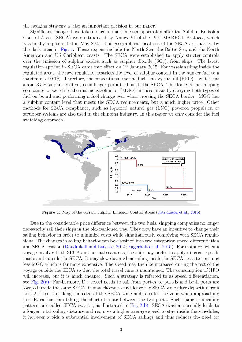
Control Areas (SECA) were introduced by Annex VI of the 1997 MARPOL Protocol, whichwas finally implemented in May 2005. The geographical locations of the SECA are marked bythe dark areas in Fig. 1. These regions include the North Sea, the Baltic Sea, and the NorthAmerican and US Caribbean coasts. The SECA were established to apply stricter controlsover the emission of sulphur oxides, such as sulphur dioxide (SO2), from ships. The latestregulation applied in SECA came into effect on 1st January 2015. For vessels sailing inside theregulated areas, the new regulation restricts the level of sulphur content in the bunker fuel to amaximum of 0.1%. Therefore, the conventional marine fuel – heavy fuel oil (HFO) – which hasabout 3.5% sulphur content, is no longer permitted inside the SECA. This forces some shippingcompanies to switch to the marine gasoline oil (MGO) in these areas by carrying both types offuel on board and performing a fuel change-over when crossing the SECA border. MGO hasa sulphur content level that meets the SECA requirements, but a much higher price. Othermethods for SECA compliance, such as liquefied natural gas (LNG) powered propulsion orscrubber systems are also used in the shipping industry. In this paper we only consider the fuelswitching approach.

Figure 1: Map of the current Sulphur Emission Control Areas (Patricksson et al., 2015)

Due to the considerable price difference between the two fuels, shipping companies no longernecessarily sail their ships in the old-fashioned way. They now have an incentive to change theirsailing behavior in order to minimize costs while simultaneously complying with SECA regula-tions. The changes in sailing behavior can be classified into two categories: speed differentiationand SECA-evasion (Doudnikoff and Lacoste, 2014; Fagerholt et al., 2015). For instance, when avoyage involves both SECA and normal sea areas, the ship may prefer to apply different speedsinside and outside the SECA. It may slow down when sailing inside the SECA so as to consumeless MGO which is far more expensive. The speed may then be increased during the rest of thevoyage outside the SECA so that the total travel time is maintained. The consumption of HFOwill increase, but it is much cheaper. Such a strategy is referred to as speed differentiation,see Fig. 2(a). Furthermore, if a vessel needs to sail from port-A to port-B and both ports arelocated inside the same SECA, it may choose to first leave the SECA zone after departing fromport-A, then sail along the edge of the SECA zone and re-enter the zone when approachingport-B, rather than taking the shortest route between the two ports. Such changes in sailingpatterns are called SECA-evasion, as illustrated in Fig. 2(b). SECA-evasion normally leads toa longer total sailing distance and requires a higher average speed to stay inside the schedules,it however avoids a substantial involvement of SECA sailings and thus reduces the need for

3

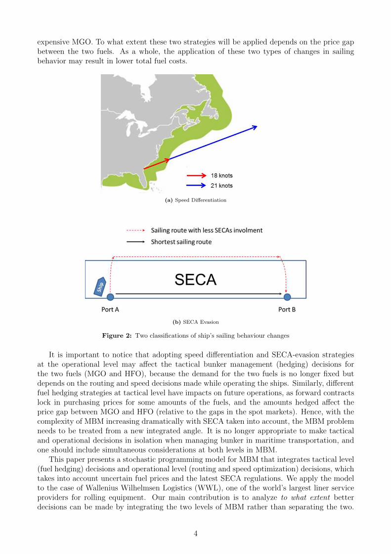
expensive MGO. To what extent these two strategies will be applied depends on the price gapbetween the two fuels. As a whole, the application of these two types of changes in sailingbehavior may result in lower total fuel costs.

(a) Speed Differentiation

(b) SECA Evasion

Figure 2: Two classifications of ship’s sailing behaviour changes

It is important to notice that adopting speed differentiation and SECA-evasion strategiesat the operational level may affect the tactical bunker management (hedging) decisions forthe two fuels (MGO and HFO), because the demand for the two fuels is no longer fixed butdepends on the routing and speed decisions made while operating the ships. Similarly, differentfuel hedging strategies at tactical level have impacts on future operations, as forward contractslock in purchasing prices for some amounts of the fuels, and the amounts hedged affect theprice gap between MGO and HFO (relative to the gaps in the spot markets). Hence, with thecomplexity of MBM increasing dramatically with SECA taken into account, the MBM problemneeds to be treated from a new integrated angle. It is no longer appropriate to make tacticaland operational decisions in isolation when managing bunker in maritime transportation, andone should include simultaneous considerations at both levels in MBM.

This paper presents a stochastic programming model for MBM that integrates tactical level(fuel hedging) decisions and operational level (routing and speed optimization) decisions, whichtakes into account uncertain fuel prices and the latest SECA regulations. We apply the modelto the case of Wallenius Wilhelmsen Logistics (WWL), one of the world’s largest liner serviceproviders for rolling equipment. Our main contribution is to analyze to what extent betterdecisions can be made by integrating the two levels of MBM rather than separating the two.

4

We also investigate how tactical and operational decisions in MBM interact with each otherafter considering uncertain fuel prices and the introduction of SECA regulations.

The paper is organized as follows. Section 2 describes the problem and the relevant as-sumptions. We then present the mathematical formulation of the model in Section 3. Section 4introduces the test case and the scenario generation process. In Section 5 we show and analyzethe results of the computational study. We then conclude in Section 6.

2 Problem description and Assumptions

In this section a detailed description of the MBM problem is given. Section 2.1 defines someimportant terms used in the paper. Section 2.2 describes the problem setting, and the relevantassumptions are stated in Section 2.3.

2.1 Terminology

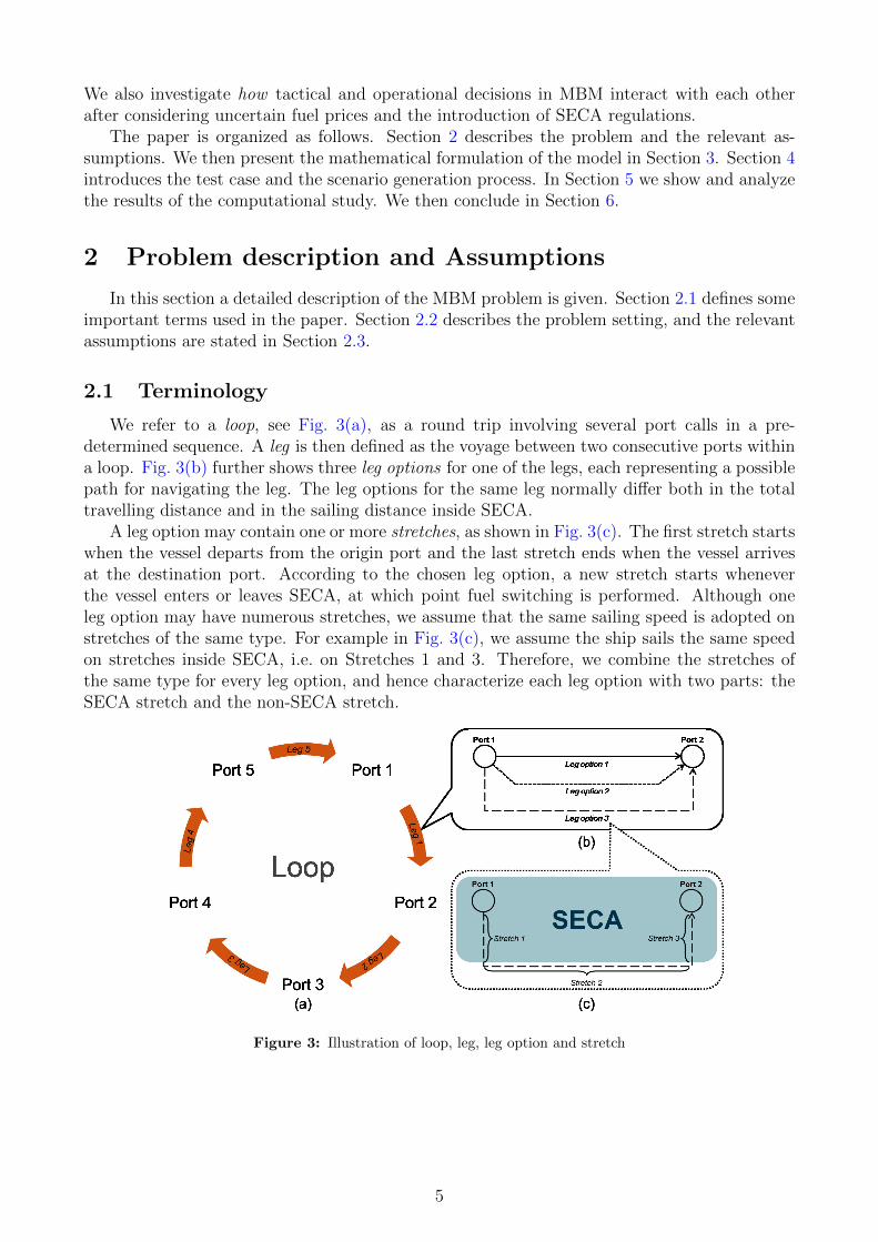
We refer to a loop, see Fig. 3(a), as a round trip involving several port calls in a pre-determined sequence. A leg is then defined as the voyage between two consecutive ports withina loop. Fig. 3(b) further shows three leg options for one of the legs, each representing a possiblepath for navigating the leg. The leg options for the same leg normally differ both in the totaltravelling distance and in the sailing distance inside SECA.

A leg option may contain one or more stretches, as shown in Fig. 3(c). The first stretch startswhen the vessel departs from the origin port and the last stretch ends when the vessel arrivesat the destination port. According to the chosen leg option, a new stretch starts wheneverthe vessel enters or leaves SECA, at which point fuel switching is performed. Although oneleg option may have numerous stretches, we assume that the same sailing speed is adopted onstretches of the same type. For example in Fig. 3(c), we assume the ship sails the same speedon stretches inside SECA, i.e. on Stretches 1 and 3. Therefore, we combine the stretches ofthe same type for every leg option, and hence characterize each leg option with two parts: theSECA stretch and the non-SECA stretch.

Figure 3: Illustration of loop, leg, leg option and stretch

5

2.2 Problem setting

A typical liner company offers services with fixed routes, schedules and frequencies, like busservices. The number of ships involved in a particular service route depends on the desiredservice frequency. Our problem is based on a trading loop operated by a liner company whichinvolves SECA sailings, and considers the company’s bunker hedging strategy as well as itsrouting, speed and fuel allocation decisions for the next planning period on the trading loop.The aim is to minimize the expected total bunker costs with uncertain fuel prices taken intoaccount, while restricting the risk in total bunker costs within a desired level.

In order to reduce their exposure to cost volatility with regards to fuel consumption, fuelhedging is the most common approach used by large fuel consumers, such as air lines and ship-ping companies. The hedging instrument considered in this paper is the forward-fuel contractwith exit terms and physical supply (FFC in the following), which is one of the most widelyused hedging tools in the shipping industry. In an FFC, the shipping company has the right topurchase a certain amount of a specified type of bunker with a fixed price during a given timeperiod, while the bunker supplier has the obligation to deliver regardless of future spot pricedevelopments. The agreed amount, price, fuel type and delivery period will be stated in thecontract. However, during the execution of an FFC, if the shipping company realizes that it nolonger needs the remaining fuel in the FFC, and decides to quit the contract, a penalty mustbe paid for the unused amount. On the other hand, the shipping company may still purchasefuel from the spot market during the operational phase in the cases where the hedged amountis not sufficient or the spot price is very low.

2.3 Assumptions

The following assumptions are made when developing the model.

• For simplicity, we only consider one ship in our problem. The length of a completeplanning period for the MBM problem is set to be the time needed for the ship to finisha round trip on a specific trading loop.

• The service network design (port visit sequence) and the corresponding leg information(such as the leg options for each leg, and the characteristics of the associated stretchesfor every leg option) of the trading loop are assumed to be given and used as input toour model.

• The unused fuel left in an FFC during the planning period cannot be stored for futureuse or sold in a spot market, but is assumed to be sold back to the bunker supplier witha certain penalty.

• The shipping company cannot enter a new FFC during the operational stage.

• The fuel market is assumed to be exogenous and transparent, in which the fuel prices arepublic information.

3 The Model

In this section we present the mathematical model for the MBM problem. Section 3.1 intro-duces several important components of the model. The mathematical formulation is presentedin Section 3.2.

6

3.1 Model development

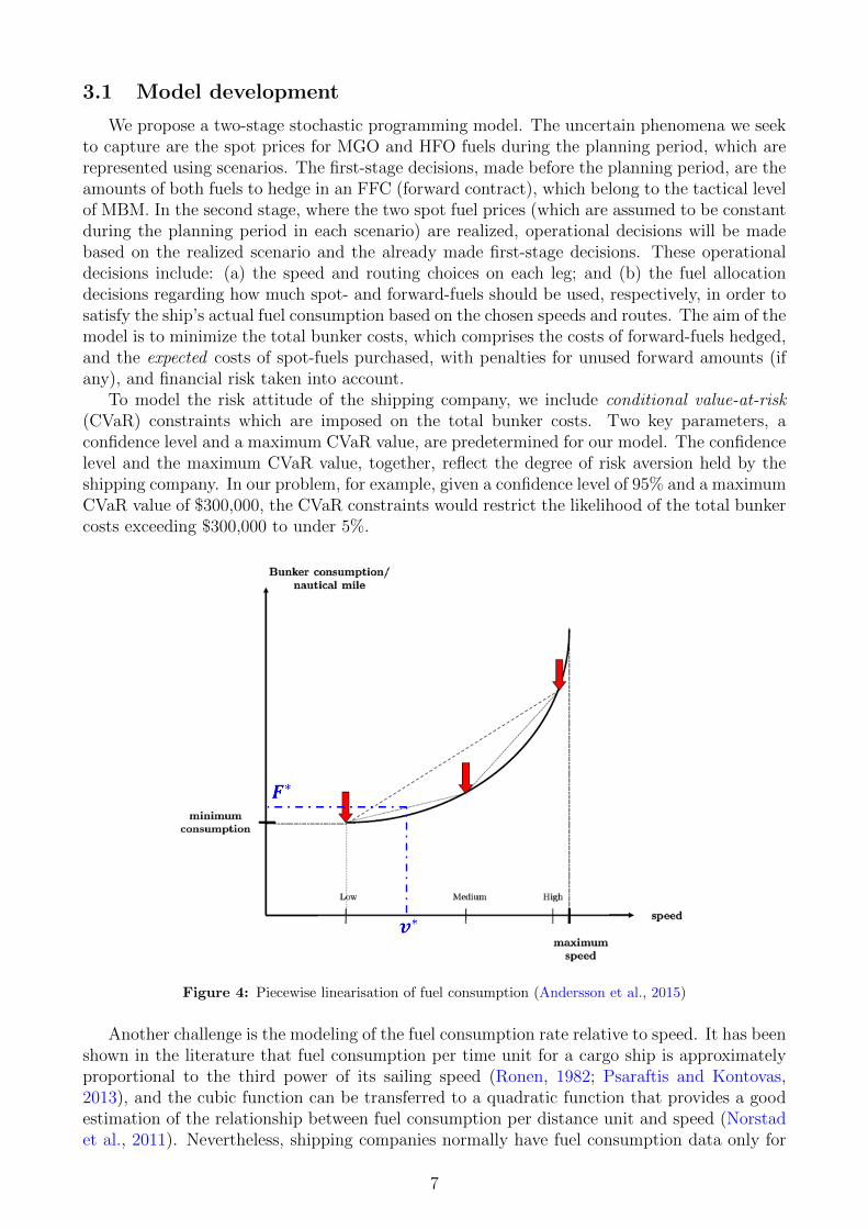
We propose a two-stage stochastic programming model. The uncertain phenomena we seekto capture are the spot prices for MGO and HFO fuels during the planning period, which arerepresented using scenarios. The first-stage decisions, made before the planning period, are theamounts of both fuels to hedge in an FFC (forward contract), which belong to the tactical levelof MBM. In the second stage, where the two spot fuel prices (which are assumed to be constantduring the planning period in each scenario) are realized, operational decisions will be madebased on the realized scenario and the already made first-stage decisions. These operationaldecisions include: (a) the speed and routing choices on each leg; and (b) the fuel allocationdecisions regarding how much spot- and forward-fuels should be used, respectively, in order tosatisfy the ship’s actual fuel consumption based on the chosen speeds and routes. The aim of themodel is to minimize the total bunker costs, which comprises the costs of forward-fuels hedged,and the expected costs of spot-fuels purchased, with penalties for unused forward amounts (ifany), and financial risk taken into account.

To model the risk attitude of the shipping company, we include conditional value-at-risk(CVaR) constraints which are imposed on the total bunker costs. Two key parameters, aconfidence level and a maximum CVaR value, are predetermined for our model. The confidencelevel and the maximum CVaR value, together, reflect the degree of risk aversion held by theshipping company. In our problem, for example, given a confidence level of 95% and a maximumCVaR value of $300,000, the CVaR constraints would restrict the likelihood of the total bunkercosts exceeding $300,000 to under 5%.

Figure 4: Piecewise linearisation of fuel consumption (Andersson et al., 2015)

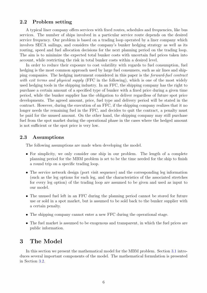
Another challenge is the modeling of the fuel consumption rate relative to speed. It has beenshown in the literature that fuel consumption per time unit for a cargo ship is approximatelyproportional to the third power of its sailing speed (Ronen, 1982; Psaraftis and Kontovas,2013), and the cubic function can be transferred to a quadratic function that provides a goodestimation of the relationship between fuel consumption per distance unit and speed (Norstadet al., 2011). Nevertheless, shipping companies normally have fuel consumption data only for

7

a group of discrete speed points rather than a function, which is also the case in our study.We therefore use the piecewise linearisation approach, proposed by Andersson et al. (2015),to approximate the fuel consumption rate under different sailing speeds. This approach useslinear combinations of the fuel consumption rates at given speed points to provide an estimationbetween these speed points, as shown in Fig. 4. For instance, if some particular speed v∗ canbe written, using two weight values a, b, a + b = 1, and two speed points vLow, vMedium, asv∗ = a ∗ vLow + b ∗ vMedium; then the estimated fuel consumption rate F ∗ at speed v∗ canbe calculated as F ∗ = a ∗ FLow + b ∗ FMedium. Although this approach normally leads to anoverestimation (see Andersson et al. for explanations), the gap is usually acceptable as long asenough discrete speed points are used. This method also gives a proper approximation of thesailing time-speed relation on each leg and stretch.

3.2 Mathematical formulation

The notation used in the formulation is as follows:

Sets

J Set of sailing legs along the loop

Rj Set of leg options for Leg j

V Set of feasible discrete speed points for the ship

S Set of price scenarios

Parameters

PMGO−F Price per ton of MGO agreed in the forward-fuel contract

PHFO−F Price per ton of HFO agreed in the forward-fuel contract

PMGO−Ss Price per ton of MGO on spot market under scenario s

PHFO−Ss Price per ton of HFO on spot market under scenario s

PMGO−P Penalty per ton for the unused MGO left in the forward-fuel contract

PHFO−P Penalty per ton for the unused HFO left in the forward-fuel contract

W j Latest starting time for Leg j

W Sj Service time for Leg j in the departing port

W SECAjrv Sailing time on SECA stretches on Leg j under Leg option r with speed v

WNjrv Sailing time on non-SECA stretches on Leg j under Leg option r with speed v

DSECAjr Sailing distance on SECA stretches on Leg j under Leg option r

DNjr Sailing distance on non-SECA stretches on Leg j under Leg option r

Fv Fuel consumption per unit distance sailed with speed alternative v (same for bothHFO and MGO)

ps Probability of scenario s taking place

γ Confidence level applied in CVaR

Aγ The maximum tolerable CVaR value under confidence level γ

8

Decision variables

xSECAjrvs Weight of speed choice v used on SECA stretches on Leg j with Leg option runder scenario s

xNjrvs Weight of speed choice v used on non-SECA stretches on Leg j with Leg optionr under scenario s

yjrs Binary variables representing the decisions on route selection, equal to 1 if Legoption r is sailed on Leg j under scenario s, and 0 otherwise

zMGO−Sjs Amount of MGO from spot market used on Leg j under scenario s

zMGO−Fjs Amount of MGO from forward contract used on Leg j under scenario s

zHFO−Sjs Amount of HFO from spot market used on Leg j under scenario s

zHFO−Fjs Amount of HFO from forward contract used on Leg j under scenario s

uMGO−Fs Amount of unused forward MGO left at the end of the planning period under

scenario s

uHFO−Fs Amount of unused forward HFO left at the end of the planning period underscenario s

mMGO−F Agreed amount of MGO in the forward contract

mHFO−F Agreed amount of HFO in the forward contract

α Artificial variable for CVaR constraints

hs Artificial variables for CVaR constraints under scenario s

The mathematical formulation is as follows:

min PMGO−FmMGO−F + PHFO−FmHFO−F

+∑s∈S

ps

{∑j∈J

(PMGO−Ss zMGO−S

js + PHFO−Ss zHFO−Sjs

)−(PMGO−F − PMGO−P )uMGO−F

s − (PHFO−F − PHFO−P )uHFO−Fs

} (1)

Subject to

W j+1 ≥ W j +W Sj +

∑r∈Rj

∑v∈V

(W SECAjrv xSECAjrvs +WN

jrvxNjrvs

)s ∈ S, j ∈ J (2)

∑v∈V

xSECAjrvs = yjrs s ∈ S, j ∈ J, r ∈ Rj (3)

∑v∈V

xNjrvs = yjrs s ∈ S, j ∈ J, r ∈ Rj (4)

∑r∈Rj

yjrs = 1 s ∈ S, j ∈ J (5)

9

zMGO−Fjs + zMGO−S

js =∑r∈Rj

∑v∈V

FvDSECAjr xSECAjrvs s ∈ S, j ∈ J (6)

zHFO−Fjs + zHFO−Sjs =∑r∈Rj

∑v∈V

FvDNjrx

Njrvs s ∈ S, j ∈ J (7)

∑j∈J

zMGO−Fjs + uMGO−F

s = mMGO−F s ∈ S (8)

∑j∈J

zHFO−Fjs + uHFO−Fs = mHFO−F s ∈ S (9)

yjrs ∈ {0, 1} s ∈ S, j ∈ J, r ∈ Rj (10)

xSECAjrvs , xNjrvs ≥ 0 s ∈ S, j ∈ J, r ∈ Rj, v ∈ V (11)

zMGO−Fjs , zMGO−S

js , zHFO−Fjs , zHFO−Sjs ≥ 0 s ∈ S, j ∈ J (12)

uMGO−Fs , uHFO−Fs ≥ 0 s ∈ S (13)

CVaR constraints:

α +1

1− γ∑s∈S

pshs ≤ Aγ (14)

hs ≥ 0 s ∈ S (15)

hs ≥ PMGO−FmMGO−F + PHFO−FmHFO−F

− (PMGO−F − PMGO−P )uMGO−Fs − (PHFO−F − PHFO−P )uHFO−Fs (16)

+∑j∈J

(PMGO−Ss zMGO−S

js + PHFO−Ss zHFO−Sjs

)− α s ∈ S

The objective function (1) minimizes the sum of the forward-fuel costs, the expected spot-fuel costs and the penalty for unused forward-fuels. The first line in the objective functionrefers to the initial costs for the agreed amounts of MGO and HFO in the forward contracts,while the expected costs for spot-fuels consumed in the second stage are expressed as the secondline of the objective function. The last line represents selling the unused forward-fuels backto the bunker supplier at the end of the planning period at their “buyback prices”, which arecalculated as their initial forward prices minus the penalty rates.

Constraints (2) ensure that the time constraints for all sailing legs are respected. Con-straints (3) and (4) connect x- and y-variables with respect to the speed-routing choices inSECA and non-SECA stretches, respectively. They ensure that the sums of the speed weights,xSECAjrvs and xNjrvs respectively for SECA and non-SECA stretches, are equal to 1 if Leg option r ischosen for Leg j in Scenario s, and 0 otherwise. Constraints (5) ensure that only one leg optionis used on any specific leg. Constraints (6) - (9) are bookkeeping constraints. Constraints (6)and (7) make sure that for each scenario the sum of the spot- and forward-fuels used on eachleg equals the actual fuel consumption on that leg based on the speeds and leg options chosen.Constraints (8) and (9) ensure that the forward-fuels used plus the leftovers equal the agreed

10

amounts in the forward contract. Constraints (10) - (13) define the domains of the decisionvariables. Constraints (14) - (16) are the CVaR constraints representing the risk (aversion)attitude of the shipping company, restricting the risk on the total bunker costs to be within anacceptable level.

4 Test case and scenario generation

In this section, we describe our test case in Section 4.1, followed by the scenario generationprocess in Section 4.2.

4.1 Basic information of the case

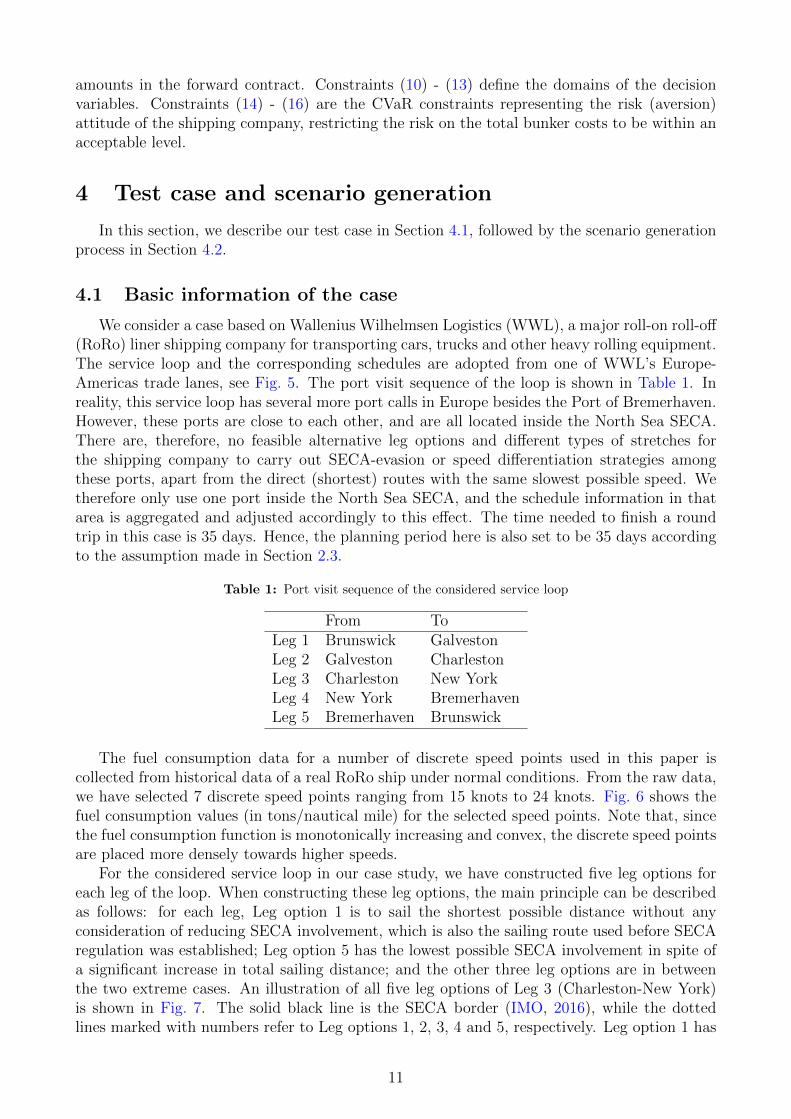
We consider a case based on Wallenius Wilhelmsen Logistics (WWL), a major roll-on roll-off(RoRo) liner shipping company for transporting cars, trucks and other heavy rolling equipment.The service loop and the corresponding schedules are adopted from one of WWL’s Europe-Americas trade lanes, see Fig. 5. The port visit sequence of the loop is shown in Table 1. Inreality, this service loop has several more port calls in Europe besides the Port of Bremerhaven.However, these ports are close to each other, and are all located inside the North Sea SECA.There are, therefore, no feasible alternative leg options and different types of stretches forthe shipping company to carry out SECA-evasion or speed differentiation strategies amongthese ports, apart from the direct (shortest) routes with the same slowest possible speed. Wetherefore only use one port inside the North Sea SECA, and the schedule information in thatarea is aggregated and adjusted accordingly to this effect. The time needed to finish a roundtrip in this case is 35 days. Hence, the planning period here is also set to be 35 days accordingto the assumption made in Section 2.3.

Table 1: Port visit sequence of the considered service loop

From ToLeg 1 Brunswick GalvestonLeg 2 Galveston CharlestonLeg 3 Charleston New YorkLeg 4 New York BremerhavenLeg 5 Bremerhaven Brunswick

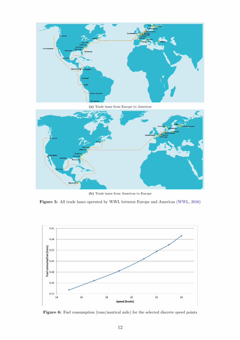
The fuel consumption data for a number of discrete speed points used in this paper iscollected from historical data of a real RoRo ship under normal conditions. From the raw data,we have selected 7 discrete speed points ranging from 15 knots to 24 knots. Fig. 6 shows thefuel consumption values (in tons/nautical mile) for the selected speed points. Note that, sincethe fuel consumption function is monotonically increasing and convex, the discrete speed pointsare placed more densely towards higher speeds.

For the considered service loop in our case study, we have constructed five leg options foreach leg of the loop. When constructing these leg options, the main principle can be describedas follows: for each leg, Leg option 1 is to sail the shortest possible distance without anyconsideration of reducing SECA involvement, which is also the sailing route used before SECAregulation was established; Leg option 5 has the lowest possible SECA involvement in spite ofa significant increase in total sailing distance; and the other three leg options are in betweenthe two extreme cases. An illustration of all five leg options of Leg 3 (Charleston-New York)is shown in Fig. 7. The solid black line is the SECA border (IMO, 2016), while the dottedlines marked with numbers refer to Leg options 1, 2, 3, 4 and 5, respectively. Leg option 1 has

11

(a) Trade lanes from Europe to Americas

(b) Trade lanes from Americas to Europe

Figure 5: All trade lanes operated by WWL between Europe and Americas (WWL, 2016)

Figure 6: Fuel consumption (tons/nautical mile) for the selected discrete speed points

12

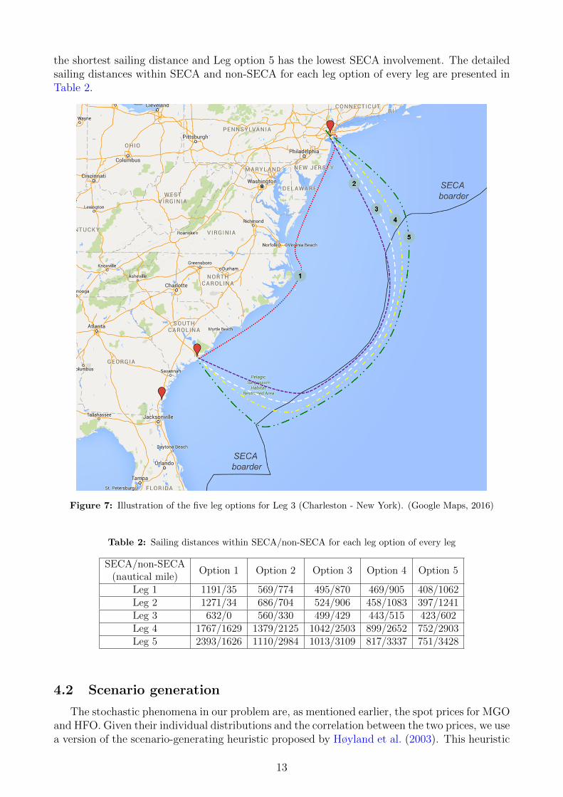
the shortest sailing distance and Leg option 5 has the lowest SECA involvement. The detailedsailing distances within SECA and non-SECA for each leg option of every leg are presented inTable 2.

Figure 7: Illustration of the five leg options for Leg 3 (Charleston - New York). (Google Maps, 2016)

Table 2: Sailing distances within SECA/non-SECA for each leg option of every leg

SECA/non-SECA(nautical mile)

Option 1 Option 2 Option 3 Option 4 Option 5

Leg 1 1191/35 569/774 495/870 469/905 408/1062Leg 2 1271/34 686/704 524/906 458/1083 397/1241Leg 3 632/0 560/330 499/429 443/515 423/602Leg 4 1767/1629 1379/2125 1042/2503 899/2652 752/2903Leg 5 2393/1626 1110/2984 1013/3109 817/3337 751/3428

4.2 Scenario generation

The stochastic phenomena in our problem are, as mentioned earlier, the spot prices for MGOand HFO. Given their individual distributions and the correlation between the two prices, we usea version of the scenario-generating heuristic proposed by Høyland et al. (2003). This heuristic

13

approach matches the first four moments of the marginal distributions plus correlations. Whenconstructing the scenarios for the spot fuel prices for the next planning period, we use thelatest observed prices on the spot market as base prices, and generate (positive or negative)price increments to be added to the base prices. The reason is that fuel prices are highlydependent over time. It would be problematic to directly use the raw data of the historical fuelprices from the past booming period (e.g. 2008) to generate future fuel price scenarios since themarket is in depression. However, the development of fuel price can be considered as a Levyprocess (Krichene, 2008; Gencer and Unal, 2012) which has independent increments.

To obtain appropriate distributions and correlation for the price increments of the two typesof fuels, we use the historical data provided by Clarkson Research Services Limited (Clarkson,2015), which is one of the largest data and consulting service providers in the shipping industry.The raw data contains the average value of the monthly prices of three major ports, Rotterdam,Houston and Singapore, from January 2000 to December 2015. Then we use the the raw datato calculate the historical monthly price increments which are used as the final input data forscenario generation process.

The correlation between the HFO and MGO price increments is estimated at 0.75, which isalso derived from the historical fuel data. Moreover, the marginal distributions of the randomprice increments are assumed to be triangular and symmetric. The marginal distributionsused in the scenario-generating heuristic are controlled by the lower limit, mode and upperlimit which are (−40, 0, 40) for HFO and (−120, 0, 120) for MGO. The symmetry, estimatedcorrelation and estimated marginal distributions are all interpreted from the monthly averageof the fuel price increments observed in the three ports during the last 16 years. For December2015, we ended up with 150 USD/ton for HFO, while for MGO it was about 375 USD/ton.These latest prices are used as the basis for the fuel price scenarios in the planning period.Since the expected values of the price increments equal 0, the expected value of the spot-fuelprices in the second stage are assumed to be equal to the latest observed fuel prices. This is areasonable assumption for our model, since if there is a known increase or decrease in expectedprices, which means a guaranteed expected gain or loss, speculation may occur and that is notwhat we analyze.

Furthermore, we also check the reliability of the scenario generation approach we use. Thein-sample stability test (Kaut and Wallace, 2007) is performed in order to ensure that thesolution of the stochastic model does not depend too much on the particular scenario tree used.We generate 10 scenario trees, each consisting of 100 scenarios, using the same generatingapproach and parameters. We then solve the problem with each scenario tree and are able toobserve approximately the same objective function values. The gap among the objective valuesin the in-sample stability test is less than 0.02%, which is small enough to ensure stability whenusing 100 scenarios in our problem.

5 Computational study

This section presents our computational study. Section 5.1 introduces the comparison andanalysis tests. Section 5.2 offers other important details applied in the computational study.Numerical results and managerial insights are given in Section 5.3.

5.1 Tested situations

In order to understand the interaction between the tactical and operational levels of MBM,and the importance of integrated decision-making, we introduce several situations in the fol-lowing, representing different types of integration between the two levels.

14

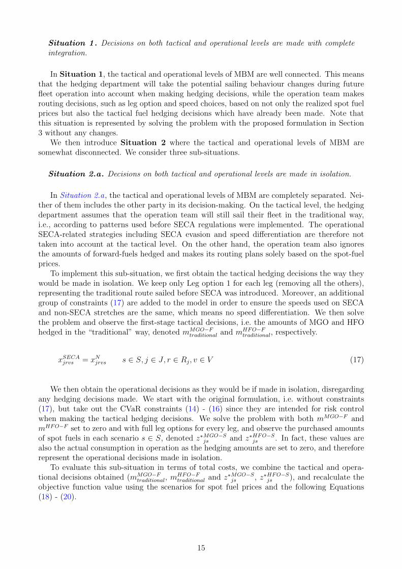
Situation 1 . Decisions on both tactical and operational levels are made with completeintegration.

In Situation 1, the tactical and operational levels of MBM are well connected. This meansthat the hedging department will take the potential sailing behaviour changes during futurefleet operation into account when making hedging decisions, while the operation team makesrouting decisions, such as leg option and speed choices, based on not only the realized spot fuelprices but also the tactical fuel hedging decisions which have already been made. Note thatthis situation is represented by solving the problem with the proposed formulation in Section3 without any changes.

We then introduce Situation 2 where the tactical and operational levels of MBM aresomewhat disconnected. We consider three sub-situations.

Situation 2.a . Decisions on both tactical and operational levels are made in isolation.

In Situation 2.a, the tactical and operational levels of MBM are completely separated. Nei-ther of them includes the other party in its decision-making. On the tactical level, the hedgingdepartment assumes that the operation team will still sail their fleet in the traditional way,i.e., according to patterns used before SECA regulations were implemented. The operationalSECA-related strategies including SECA evasion and speed differentiation are therefore nottaken into account at the tactical level. On the other hand, the operation team also ignoresthe amounts of forward-fuels hedged and makes its routing plans solely based on the spot-fuelprices.

To implement this sub-situation, we first obtain the tactical hedging decisions the way theywould be made in isolation. We keep only Leg option 1 for each leg (removing all the others),representing the traditional route sailed before SECA was introduced. Moreover, an additionalgroup of constraints (17) are added to the model in order to ensure the speeds used on SECAand non-SECA stretches are the same, which means no speed differentiation. We then solvethe problem and observe the first-stage tactical decisions, i.e. the amounts of MGO and HFOhedged in the “traditional” way, denoted mMGO−F

traditional and mHFO−Ftraditional, respectively.

xSECAjrvs = xNjrvs s ∈ S, j ∈ J, r ∈ Rj, v ∈ V (17)

We then obtain the operational decisions as they would be if made in isolation, disregardingany hedging decisions made. We start with the original formulation, i.e. without constraints(17), but take out the CVaR constraints (14) - (16) since they are intended for risk controlwhen making the tactical hedging decisions. We solve the problem with both mMGO−F andmHFO−F set to zero and with full leg options for every leg, and observe the purchased amountsof spot fuels in each scenario s ∈ S, denoted z∗MGO−S

js and z∗HFO−Sjs . In fact, these values arealso the actual consumption in operation as the hedging amounts are set to zero, and thereforerepresent the operational decisions made in isolation.

To evaluate this sub-situation in terms of total costs, we combine the tactical and opera-tional decisions obtained (mMGO−F

traditional, mHFO−Ftraditional and z∗MGO−S

js , z∗HFO−Sjs ), and recalculate theobjective function value using the scenarios for spot fuel prices and the following Equations(18) - (20).

15

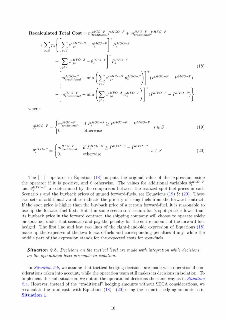
Recalculated Total Cost = mMGO−FtraditionalP

MGO−F +mHFO−FtraditionalP

HFO−F

+∑s∈S

ps

{[∑j∈J

z∗MGO−Sjs − θMGO−F

s

]+

PMGO−Ss

+

[∑j∈J

z∗HFO−Sjs − θHFO−Fs

]+

PHFO−Ss

−

[mMGO−Ftraditional −min

(∑j∈J

z∗MGO−Sjs , θMGO−F

s

)]+

(PMGO−F − PMGO−P )

−

[mHFO−Ftraditional −min

(∑j∈J

z∗HFO−Sjs , θHFO−Fs

)]+

(PHFO−F − PHFO−P )

}(18)

where

θMGO−Fs =

{mMGO−Ftraditional, if PMGO−S

s ≥ PMGO−F − PMGO−P

0, otherwise, s ∈ S (19)

θHFO−Fs =

{mHFO−Ftraditional, if PHFO−S

s ≥ PHFO−F − PHFO−P

0, otherwise, s ∈ S (20)

The [ ]+ operator in Equation (18) outputs the original value of the expression insidethe operator if it is positive, and 0 otherwise. The values for additional variables θMGO−F

s

and θHFO−Fs are determined by the comparison between the realized spot-fuel prices in eachScenario s and the buyback prices of unused forward-fuels, see Equations (19) & (20). Thesetwo sets of additional variables indicate the priority of using fuels from the forward contract.If the spot price is higher than the buyback price of a certain forward-fuel, it is reasonable touse up the forward-fuel first. But if in some scenario a certain fuel’s spot price is lower thanits buyback price in the forward contract, the shipping company will choose to operate solelyon spot-fuel under that scenario and pay the penalty for the entire amount of the forward-fuelhedged. The first line and last two lines of the right-hand-side expression of Equations (18)make up the expenses of the two forward-fuels and corresponding penalties if any, while themiddle part of the expression stands for the expected costs for spot-fuels.

Situation 2.b. Decisions on the tactical level are made with integration while decisionson the operational level are made in isolation.

In Situation 2.b, we assume that tactical hedging decisions are made with operational con-siderations taken into account, while the operation team still makes its decisions in isolation. Toimplement this sub-situation, we obtain the operational decisions the same way as in Situation2.a. However, instead of the “traditional” hedging amounts without SECA considerations, werecalculate the total costs with Equations (18) - (20) using the “smart” hedging amounts as inSituation 1.

16

Situation 2.c. Decisions on the tactical level are made in isolation while decisions onthe operational levels are made with integration.

In Situation 2.c, the tactical hedging decisions are made assuming “traditional” sailingpatterns, but the operation team optimizes its sailings in the light of both SECA considerationand the hedging decisions already made. To implement, we set the variables mMGO−F andmHFO−F to mMGO−F

traditional and mHFO−Ftraditional, respectively, which are the “traditional” amounts of

MGO and HFO hedged as obtained in Situation 2.a. We then solve the problem (without theCVaR constraints), and observe the objective function value.

5.2 Other important details

Before we show the numerical results, some other important details applied in the compu-tational study must be stated.

In all tested situations the forward price is set to be slightly higher than the expected valueof the stochastic spot price over the planning period, which means there is no free lunch forremoving the risks. Moreover, the penalty levels for both fuels are ideally set so that only riskaverse companies will buy FFC.

In order to ensure the comparability of different situations, we apply the same level ofrisk aversion in all of our tests, whenever the CVaR constraints (14) - (16) are active. Themaximum CVaR value (Aγ) is set to be 1% higher than the expected costs obtained under arisk neutral assumption 1, and the confidence value (γ) is set to 95%. These parameters canof course be adjusted according to the shipping company’s actual risk attitude. However, sincethe minimized expected costs in the risk neutral case are the lowest costs that the shippingcompany can get, we argue that restricting the total costs in the extreme cases to a maximumof 1% increase is a reasonable risk control setting for the test purpose in this paper.

5.3 Numerical results

The aggregated numerical results for all tested situations are displayed in Table 3. For eachsituation, the first-stage hedging decisions as well as the (average) second-stage fuel allocationdecisions are presented in detail.

The average consumption of different fuels equals the sum of the actual fuel consumptionof that type in each scenario multiplied by the probability of the scenario. Similar logic appliesto the average unused fuels. Moreover, the expected total costs is the objective value of theoptimization while the standard deviation refers to the cost volatility among all the scenarios.Given a 95% confidence level, the last row in the table shows the risk level in extreme cases(CVaR value) which equals the average of the realized total costs in the worst 5% scenarios inthat situation.

5.3.1 Comparison between Situation 1 and Situation 2.a

To compare Situation 2.a with Situation 1, we use a box plot to show the scope andvariability of the total costs produced across all 100 scenarios for each of the two situations,see Fig. 8. The whisker on either side of a box represents the 5% scenarios with the highest(right whisker) or the lowest (left whisker) total costs, while the box represents the remaining

1Since the forward-fuel prices are only set marginally higher than the expected prices of the spot-fuels, it isfeasible and reasonable to restrict the risk level to such extent in this test. We also need to point out that thecomparison between risk neutral and risk averse cases is not the focus of this paper.

17

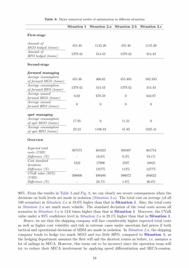
Table 3: Major numerical results of optimization in different situations

Situation 1 Situation 2.a Situation 2.b Situation 2.c

First-stage

Amount ofMGO hedged (tonne)

455.40 1145.20 455.40 1145.20

Amount ofHFO hedged (tonne)

1379.42 314.43 1379.42 314.43

Second-stage

forward managingAverage consumptionof forward MGO (tonne)

455.38 466.62 455.403 502.333

Average consumptionof forward HFO (tonne)

1379.42 314.43 1379.42 314.43

Average unusedforward MGO (tonne)

0.02 678.59 0 642.87

Average unusedforward HFO (tonne)

0 0 0 0

spot managingAverage consumptionof spot MGO (tonne)

17.95 0 11.21 0

Average consumptionof spot HFO (tonne)

23.24 1106.83 41.83 1025.41

Overview

Expected totalcosts (USD)

387575 464323 388567 461754

Difference (%) - 19.8% 0.3% 19.1%Cost standarddeviation

1222 17806 2597 16825

Difference (%) - 1357% 113% 1277%CVaR value (95%)(USD)

390000 499486 396072 494622

Difference (%) - 28.1% 1.6% 26.8%

90%. From the results in Table 3 and Fig. 8, we can clearly see severe consequences when thedecisions on both levels are made in isolation (Situation 2.a). The total cost on average (of all100 scenarios) in Situation 2.a is 19.8% higher than that in Situation 1. Also, the total costsin Situation 2.a are much more volatile. The standard deviation of the total costs across allscenarios in Situation 2.a is 13.6 times higher than that in Situation 1. Moreover, the CVaRvalue under a 95% confidence level in Situation 2.a is 28.1% higher than that in Situation 1.

Hence, we see that the shipping company will face considerably higher expected total costsas well as higher cost volatility and risk in extreme cases under uncertain fuel prices if bothtactical and operational decisions of MBM are made in isolation. In Situation 2.a, the shippingcompany tends to hedge too much MGO and too little HFO, compared to Situation 1, asthe hedging department assumes the fleet will sail the shortest routes as before, i.e. assumes alot of sailings in SECA. However, this turns out to be incorrect since the operation team willtry to reduce their SECA involvement by applying speed differentiation and SECA-evasion.

18

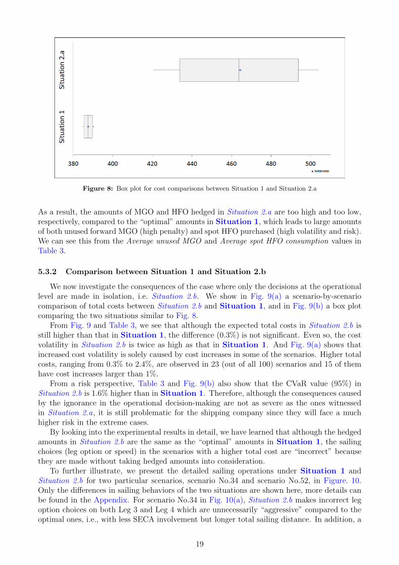
Figure 8: Box plot for cost comparisons between Situation 1 and Situation 2.a

As a result, the amounts of MGO and HFO hedged in Situation 2.a are too high and too low,respectively, compared to the “optimal” amounts in Situation 1, which leads to large amountsof both unused forward MGO (high penalty) and spot HFO purchased (high volatility and risk).We can see this from the Average unused MGO and Average spot HFO consumption values inTable 3.

5.3.2 Comparison between Situation 1 and Situation 2.b

We now investigate the consequences of the case where only the decisions at the operationallevel are made in isolation, i.e. Situation 2.b. We show in Fig. 9(a) a scenario-by-scenariocomparison of total costs between Situation 2.b and Situation 1, and in Fig. 9(b) a box plotcomparing the two situations similar to Fig. 8.

From Fig. 9 and Table 3, we see that although the expected total costs in Situation 2.b isstill higher than that in Situation 1, the difference (0.3%) is not significant. Even so, the costvolatility in Situation 2.b is twice as high as that in Situation 1. And Fig. 9(a) shows thatincreased cost volatility is solely caused by cost increases in some of the scenarios. Higher totalcosts, ranging from 0.3% to 2.4%, are observed in 23 (out of all 100) scenarios and 15 of themhave cost increases larger than 1%.

From a risk perspective, Table 3 and Fig. 9(b) also show that the CVaR value (95%) inSituation 2.b is 1.6% higher than in Situation 1. Therefore, although the consequences causedby the ignorance in the operational decision-making are not as severe as the ones witnessedin Situation 2.a, it is still problematic for the shipping company since they will face a muchhigher risk in the extreme cases.

By looking into the experimental results in detail, we have learned that although the hedgedamounts in Situation 2.b are the same as the “optimal” amounts in Situation 1, the sailingchoices (leg option or speed) in the scenarios with a higher total cost are “incorrect” becausethey are made without taking hedged amounts into consideration.

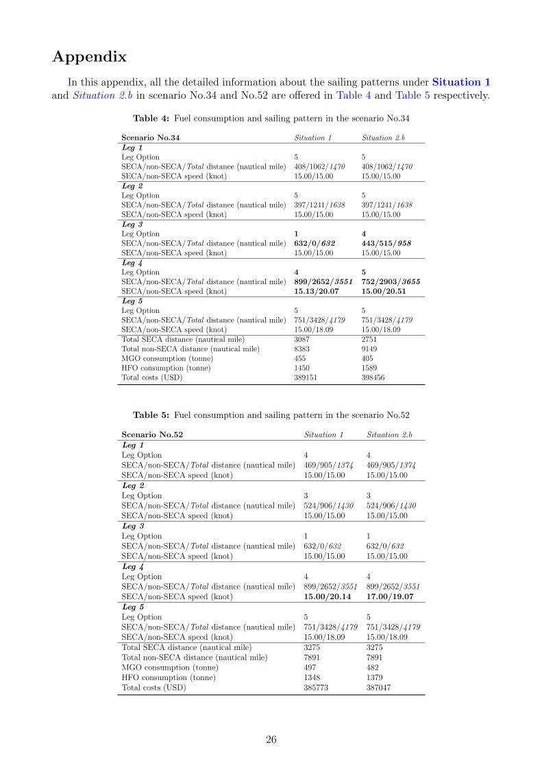
To further illustrate, we present the detailed sailing operations under Situation 1 andSituation 2.b for two particular scenarios, scenario No.34 and scenario No.52, in Figure. 10.Only the differences in sailing behaviors of the two situations are shown here, more details canbe found in the Appendix. For scenario No.34 in Fig. 10(a), Situation 2.b makes incorrect legoption choices on both Leg 3 and Leg 4 which are unnecessarily “aggressive” compared to theoptimal ones, i.e., with less SECA involvement but longer total sailing distance. In addition, a

19

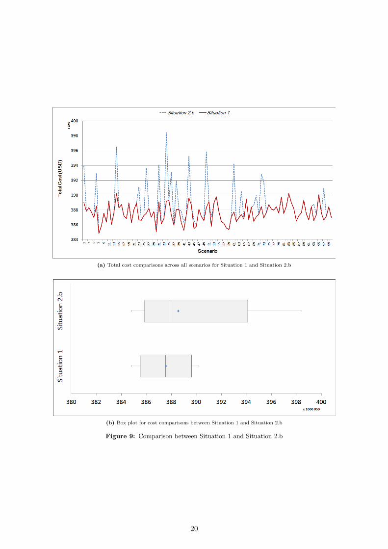
(a) Total cost comparisons across all scenarios for Situation 1 and Situation 2.b

(b) Box plot for cost comparisons between Situation 1 and Situation 2.b

Figure 9: Comparison between Situation 1 and Situation 2.b

20

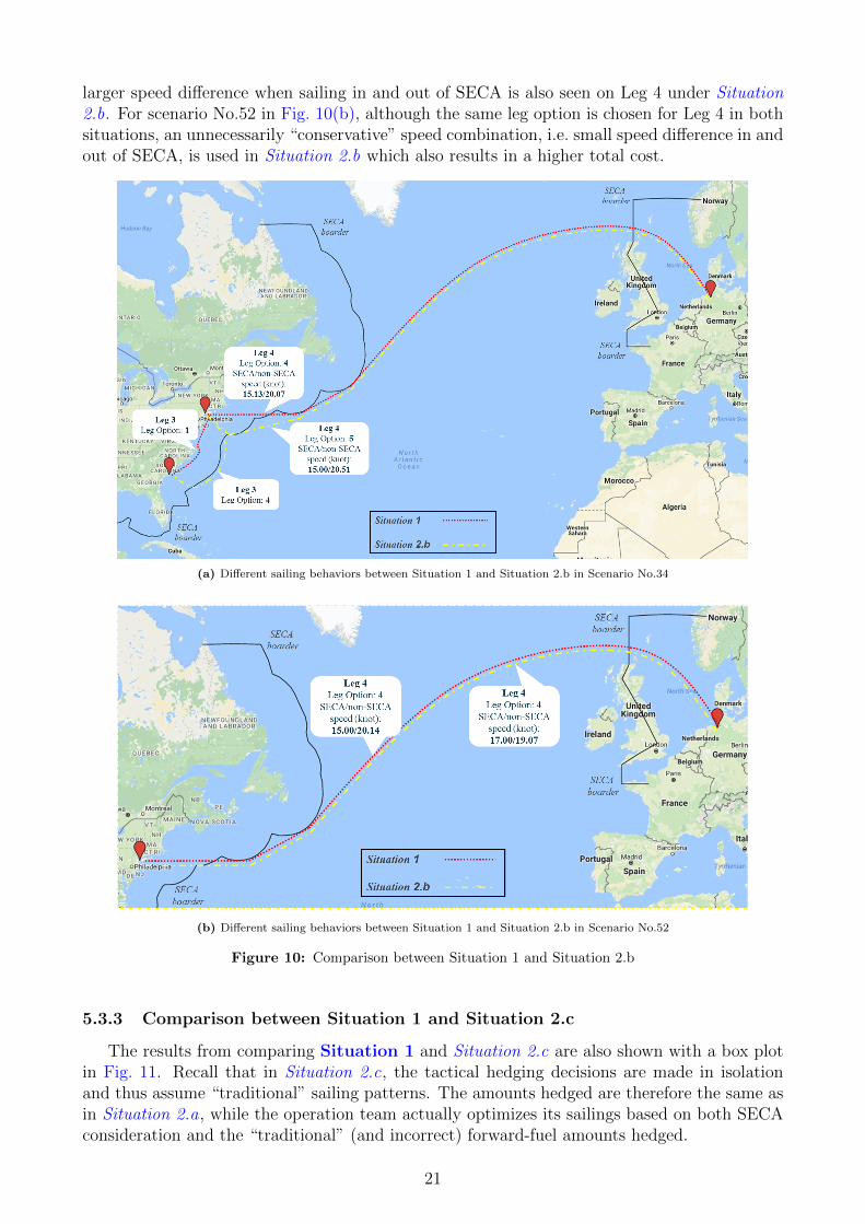
larger speed difference when sailing in and out of SECA is also seen on Leg 4 under Situation2.b. For scenario No.52 in Fig. 10(b), although the same leg option is chosen for Leg 4 in bothsituations, an unnecessarily “conservative” speed combination, i.e. small speed difference in andout of SECA, is used in Situation 2.b which also results in a higher total cost.

(a) Different sailing behaviors between Situation 1 and Situation 2.b in Scenario No.34

(b) Different sailing behaviors between Situation 1 and Situation 2.b in Scenario No.52

Figure 10: Comparison between Situation 1 and Situation 2.b

5.3.3 Comparison between Situation 1 and Situation 2.c

The results from comparing Situation 1 and Situation 2.c are also shown with a box plotin Fig. 11. Recall that in Situation 2.c, the tactical hedging decisions are made in isolationand thus assume “traditional” sailing patterns. The amounts hedged are therefore the same asin Situation 2.a, while the operation team actually optimizes its sailings based on both SECAconsideration and the “traditional” (and incorrect) forward-fuel amounts hedged.

21

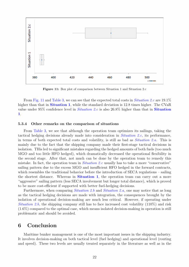
Figure 11: Box plot of comparison between Situation 1 and Situation 2.c

From Fig. 11 and Table 3, we can see that the expected total costs in Situation 2.c are 19.1%higher than that in Situation 1, while the standard deviation is 12.8 times higher. The CVaRvalue under 95% confidence level in Situation 2.c is also 26.8% higher than that in Situation1.

5.3.4 Other remarks on the comparison of situations

From Table 3, we see that although the operation team optimizes its sailings, taking thetactical hedging decisions already made into consideration in Situation 2.c, its performance,in terms of both expected total costs and volatility, is still as bad as Situation 2.a. This ismainly due to the fact that the shipping company made their first-stage tactical decisions inisolation. THis led to significant mistakes regarding the hedged amounts of both fuels (too muchMGO and too little HFO hedged), which dramatically decreased the operational flexibility inthe second stage. After that, not much can be done by the operation team to remedy thismistake. In fact, the operation team in Situation 2.c usually has to take a more “conservative”sailing pattern due to the excess MGO and insufficient HFO hedged in the forward contracts,which resembles the traditional behavior before the introduction of SECA regulations – sailingthe shortest distance. Whereas in Situation 1, the operation team can carry out a more“aggressive” sailing pattern (less SECA involvement but longer total distance), which is provedto be more cost-efficient if supported with better fuel-hedging decisions.

Furthermore, when comparing Situation 2.b and Situation 2.a, one may notice that as longas the tactical hedging decisions are made with integration, the consequences brought by theisolation of operational decision-making are much less critical. However, if operating underSituation 2.b, the shipping company still has to face increased cost volatility (110%) and risk(1.6%) compared to the optimal case, which means isolated decision-making in operation is stillproblematic and should be avoided.

6 Conclusion

Maritime bunker management is one of the most important issues in the shipping industry.It involves decision-making on both tactical level (fuel hedging) and operational level (routingand speed). These two levels are usually treated separately in the literature as well as in the

22

industry. After the latest SECA regulation came into force, the complexity of MBM increaseddramatically. The new challenges include not only the involvement of the expensive MGOrequired for the voyages inside SECA but also the possible changes in sailing behavior inducedby the price gap between MGO and the traditional bunker HFO which can still be used outsideSECA. Therefore we study the MBM problem with a new integrated point of view.

In this paper, we have proposed a stochastic programming model integrating the tacticaland operational levels of MBM, taking SECA into account. We utilize the model to explore howthe tactical and operational decisions in the problem interact. Through a computational studywe have pointed out that the tactical and operational levels in MBM do affect and interact witheach other. Isolated decision-making on either tactical or operational level in MBM will leadto various problems such as higher expected total costs, higher cost volatility and higher risk.However, the most critical situation is when tactical decisions are made in isolation. Therefore,it is important for the shipping company to have an integrated approach to MBM in light ofSECA. Such an integrated view is standard in most businesses, but was not necessary in MBMbefore the introduction of SECA.

This work has two major contributions. Firstly, it fills a gap in the present literature,where only very few studies include and integrate both tactical and operational considerationsin MBM. Secondly, it demonstrates that tactical and operational decisions must be integratedin MBM after SECA regulations were introduced, and shows the consequences for a companyif the integration does not happen.

Acknowledgments

The authors acknowledge financial support from the project “Green shipping under uncer-tainty (GREENSHIPRISK)” partly funded by the Research Council of Norway under grantnumber 233985.

References

Alizadeh, A. H., Kavussanos, M. G., and Menachof, D. A. (2004). Hedging against bunkerprice fluctuations using petroleum futures contracts: constant versus time-varying hedgeratios. Applied Economics, 36(12):1337–1353.

Andersson, H., Fagerholt, K., and Hobbesland, K. (2015). Integrated maritime fleet deploymentand speed optimization: case study from roro shipping. Computers & Operations Research,55:233–240.

Christiansen, M., Fagerholt, K., and RonenShip, D. (2004). Routing and scheduling: Statusand perspectives. Transportation Science, 38(1):1–18.

Clarkson (2015). Clarkson Research Services website. https://sin.clarksons.net/. (accessed11.01.2016).

Doudnikoff, M. and Lacoste, R. (2014). Effect of a speed reduction of containerships in responseto higher energy costs in sulphur emission control areas. Transportation Research Part D,28:51–61.

Fagerholt, K., Gausel, N. T., Rakke, J. G., and Psaraftis, H. N. (2015). Maritime routing andspeed optimization with emission control areas. Transportation Research Part C, 52:57–73.

23

Fagerholt, K., Laporte, G., and Norstad, I. (2010). Reducing fuel emissions by optimizing speedon shipping routes. Journal of the Operational Research Society, 61(3):523–529.

Gencer, M. and Unal, G. (2012). Crude oil price modelling with Levy process. InternationalJournal of Economics and Finance Studies, 4(2):139–148.

Ghosh, S., Lee, L. H., and Ng, S. H. (2015). Bunkering decisions for a shipping liner in anuncertain environment with service contract. European Journal of Operational Research,244:792–802.

Hoff, A., Andersson, H., Christiansen, M., Hasle, G., and Løkketangen, A. (2010). Industrialaspects and literature survey: Fleet composition and routing. Computers & OperationsResearch, 37(12):2041–2061.

Høyland, K., Kaut, M., and Wallace, S. W. (2003). A heuristic for moment-matching scenariogeneration. Computational optimization and applications, 24(2):169–185.

ICS (2015). International Chamber of Shipping website. http://www.ics-shipping.org/shipping-facts/shipping-and-world-trade. (accessed 05.02.2016).

IMO (2016). International Maritime Organization website. http://www.imo.org/en/OurWork/Environment/PollutionPrevention/AirPollution/Pages/Emission-Control-Areas-

(ECAs)-designated-under-regulation-13-of-MARPOL-Annex-VI-(NOx-emission-

control).aspx. (accessed 05.02.2016).

Kaut, M. and Wallace, S. W. (2007). Evaluation of scenario-generation methods for stochasticprogramming. Pacific Journal of Optimization, 3(2):257–271.

Krichene, N. (2008). Crude oil prices: Trends and forecast. Working Paper WP/08/133,International Monetary Fund.

Lindstad, H., Asbjørnslett, B. E., and Strømman, A. H. (2011). Reductions in greenhouse gasemissions and cost by shipping at lower speeds. Energy Policy, 39(6):3456–3464.

Menachof, D. A. and Dicer, G. N. (2001). Risk management methods for the liner ship-ping industry: the case of the bunker adjustment factor. Maritime Policy & Management,28(2):141–155.

Meng, Q., Wang, S., Andersson, H., and Thun, K. (2013). Containership routing and schedulingin liner shipping: Overview and future research directions. Transportation Science, 48(2):265–280.

Norstad, I., Fagerholt, K., and Laporte, G. (2011). Tramp ship routing and scheduling withspeed optimization. Transportation Research Part C, 19(5):853–865.

Patricksson, Ø. S., Fagerholt, K., and Rakke, J. G. (2015). The fleet renewal problem withregional emission limitations: Case study from roll-on/roll-off shipping. Transportation Re-search Part C, 56:346–358.

Pedrielli, G., Lee, L. H., and Ng, S. H. (2015). Optimal bunkering contract in a buyersellersupply chain under price and consumption uncertainty. Transportation Research Part E,77:77–94.

Plum, C. E. M., Jensen, P. N., and Pisinger, D. (2014). Bunker purchasing with contracts.Maritime Economics & Logistics, 16:418–435.

24

Prodhon, C. and Prins, C. (2014). A survey of recent research on location-routing problems.European Journal of Operational Research, 238:1–17.

Psaraftis, H. N. and Kontovas, C. A. (2010). Balancing the economic and environmentalperformance of maritime transportation. Transportation Research Part D, 15(8):458–462.

Psaraftis, H. N. and Kontovas, C. A. (2013). Speed models for energy-efficient maritime trans-portation: A taxonomy and survey. Transportation Research Part C, 26:331–351.

Ronen, D. (1982). The effect of oil price on the optimal speed of ships. Journal of the OperationalResearch Society, 33(11):1035–1040.

Ronen, D. (2011). The effect of oil price on containership speed and fleet size. Journal of theOperational Research Society, 62(1):211–216.

Stopford, M. (2009). Maritime Economics, page 225. London: Routledge, 3rd edition.

Wang, S. and Meng, Q. (2012). Sailing speed optimization for container ships in a liner shippingnetwork. Transportation Research Part E, 48(3):701–714.

Wang, S. and Meng, Q. (2015). Robust bunker management for liner shipping networks.European Journal of Operational Research, 243(3):789–797.

Wang, S., Meng, Q., and Liu, Z. (2013). Bunker consumption optimization methods in shipping:A critical review and extensions. Transportation Research Part E, 53:49–62.

Wang, X. and Teo, C. C. (2013). Integrated hedging and network planning for containershipping’s bunker fuel management. Maritime Economics & Logistics, 15(2):172–196.

WWL (2016). Wallenius Wilhelmsen Logistics website. http://www.2wglobal.com/global-network/. (accessed 19.02.2016).

Xia, J., Li, K. X., Ma, H., and Xu, Z. (2015). Joint planning of fleet deployment, speedoptimization, and cargo allocation for liner shipping. Transportation Science, 49(4):922–938.

Yao, Z., Ng, S. H., and Lee, L. H. (2012). A study on bunker fuel management for the shippingliner services. Computers and Operations Research, 39(5):1160–1172.

25

Appendix

In this appendix, all the detailed information about the sailing patterns under Situation 1and Situation 2.b in scenario No.34 and No.52 are offered in Table 4 and Table 5 respectively.

Table 4: Fuel consumption and sailing pattern in the scenario No.34

Scenario No.34 Situation 1 Situation 2.bLeg 1Leg Option 5 5SECA/non-SECA/Total distance (nautical mile) 408/1062/1470 408/1062/1470SECA/non-SECA speed (knot) 15.00/15.00 15.00/15.00Leg 2Leg Option 5 5SECA/non-SECA/Total distance (nautical mile) 397/1241/1638 397/1241/1638SECA/non-SECA speed (knot) 15.00/15.00 15.00/15.00Leg 3Leg Option 1 4SECA/non-SECA/Total distance (nautical mile) 632/0/632 443/515/958SECA/non-SECA speed (knot) 15.00/15.00 15.00/15.00Leg 4Leg Option 4 5SECA/non-SECA/Total distance (nautical mile) 899/2652/3551 752/2903/3655SECA/non-SECA speed (knot) 15.13/20.07 15.00/20.51Leg 5Leg Option 5 5SECA/non-SECA/Total distance (nautical mile) 751/3428/4179 751/3428/4179SECA/non-SECA speed (knot) 15.00/18.09 15.00/18.09Total SECA distance (nautical mile) 3087 2751Total non-SECA distance (nautical mile) 8383 9149MGO consumption (tonne) 455 405HFO consumption (tonne) 1450 1589Total costs (USD) 389151 398456

Table 5: Fuel consumption and sailing pattern in the scenario No.52

Scenario No.52 Situation 1 Situation 2.bLeg 1Leg Option 4 4SECA/non-SECA/Total distance (nautical mile) 469/905/1374 469/905/1374SECA/non-SECA speed (knot) 15.00/15.00 15.00/15.00Leg 2Leg Option 3 3SECA/non-SECA/Total distance (nautical mile) 524/906/1430 524/906/1430SECA/non-SECA speed (knot) 15.00/15.00 15.00/15.00Leg 3Leg Option 1 1SECA/non-SECA/Total distance (nautical mile) 632/0/632 632/0/632SECA/non-SECA speed (knot) 15.00/15.00 15.00/15.00Leg 4Leg Option 4 4SECA/non-SECA/Total distance (nautical mile) 899/2652/3551 899/2652/3551SECA/non-SECA speed (knot) 15.00/20.14 17.00/19.07Leg 5Leg Option 5 5SECA/non-SECA/Total distance (nautical mile) 751/3428/4179 751/3428/4179SECA/non-SECA speed (knot) 15.00/18.09 15.00/18.09Total SECA distance (nautical mile) 3275 3275Total non-SECA distance (nautical mile) 7891 7891MGO consumption (tonne) 497 482HFO consumption (tonne) 1348 1379Total costs (USD) 385773 387047

26