Institute of Mechanics

Software Supported Implementation ofEfficient Solid-Shell Finite Elements

September 2010

Steffen Mattern, Karl Schweizerhof

Institute of MechanicsKaiserstr. 12

D-76131 KarlsruheTel.: +49 (0) 721/ 608-2071Fax: +49 (0) 721/608-7990

E-Mail: info@ifm.kit.eduwww.ifm.uni-karlsruhe.de

KIT – University of the State of Baden-Wuerttemberg and National Laboratory of the Helmholtz Association www.kit.edu

Software Supported Implementation of EfficientSolid-Shell Finite Elements

Steffen Mattern Karl Schweizerhof

Abstract

The operations necessary for the computation of the internal nodal force vector are ingeneral the most time-consuming parts of an explicit FE-analysis. The paper presents animplementation concept for element routines for volumetric shell – the so-called Solid-Shell – elements based on the application of the symbolic programming tool ACEGEN, aplug-in for the computer algebra software MATHEMATICA . This symbolic implementationmeans that vector and matrix operations and differentiations do not have to be computedin advance in order to realize a conversion into a programming language. Consequently,programming errors can be avoided almost completely and less time is required for theimplementation. Program code in FORTRAN is generated and simultaneously optimizedautomatically, which leads to very efficient routines compared to manually implementedcode.

1 Introduction

In order to realize a continuum-like modeling of a shell structure and being able to to capture3D effects as in laminated shells, the so-called Solid-Shell element class, presented e.g. in[18, 11], with linear interpolation of geometry and displacements in thickness as well as inshell surface direction is a suitable alternative to purely3D analysis. As the formulation allowsindependent interpolation for the in-plane and the out-of-plane direction, a separate higher orderinterpolation only in the shell-surface plane as often needed for arbitrary curved shell geometriesis possible.

The most widely-used explicit time integration method is the central difference scheme,often also called VERLET algorithm [24]. For lumped mass matrices the costly solution ofcoupled linear equations on global level is not necessary; further the usage of diagonalizedmass matrices solely requires vector operations, which leads to low computational cost per timestep. Unfortunately, due to the so-called COURANT criterion [8], the time step size is limited to acritical value, which makes the central difference method mostly attractive for ‘highly dynamic’problems like impact, strong nonlinearities and short duration transient analyses, where smalltime steps are required anyway.

In this contribution the focus is on an implementation concept for Solid-Shell elements us-ing linear/ quadratic interpolation of geometry and displacements in in-plane direction togetherwith a linear interpolation in thickness direction. Besides the pure displacement formulationwith standard (full) numerical integration, which – as is well-known – leads to an overly stiffbehavior, the implementation of different approaches in order to reduce these so-called lockingphenomena are discussed. Regarding geometric locking effects, the method of ‘Assumed Nat-ural Strains’ (ANS) [2, 6, 4, 5], where the strains are evaluated at specific sampling points and

2

interpolated with the desired order is applied. POISSON locking, which affects simulations nearthe incompressible limit is cured with different versions (i. e. different numbers of parameters)of the ‘Enhanced Assumed Strain’ (EAS) method [23, 22].

The implementation concept is based on the application of the symbolic programming toolACEGEN, q.v. [15, 13], which allows a combination of symbolic operations together with theautomatic generation of highly efficient program code. BothANS and EAS schemes are alsoimplemented applying symbolic programming. The generatedsubroutines are implementedinto the in-house finite element code FEAP-MeKa [21]. The specifics of the implementationconcept are discussed and the efficiency and functionality of the element formulations are pre-sented on numerical examples.

2 Explicit Time Integration

For numerical time integration, the well-known central difference method is used and imple-mented as proposed e. g. in [3] or originally for molecular dynamics in [24]. Here the governingequations are shown briefly.

For the current time stepn, the accelerations are computed as

dn = M

−1(

fn −C d

n−1/2)

, (1)

with the diagonalized system mass matrixM, the system load vectorfn at timen, the systemdamping matrixC and the velocitiesdn−1/2 at time stepn− 1/2. The velocity between two timesteps is updated by

dn+1/2 = d

n−1/2 + ∆tn dn (2)

with ∆tn = (∆tn+∆tn−1)2

, which leads to the displacements

dn+1 = d

n + ∆tn dn+1/2, (3)

with the current time step size∆tn = tn+1− tn. The time step size is limited by the COURANT-criterion by

∆t ≤ α ∆tcrit = α2

ωmax

≈ α

(

mine

lece

)

, (4)

whereωmax is the largest eigenfrequency,le represents a characteristic element length andce thewave propagation velocity. The COURANT-criterion is based on linear problems, so in order toconsider non-linearities, the factorα < 1 is introduced. For moderately non-linear application,usuallyα = 0.9 is sufficient, for applications as e. g. high-speed impact problems,α may haveto be0.9 or even less.

The implementation of the central difference method leads to a system of uncoupled linearequations and only vector operations are performed on global level if diagonal mass matricesare used. This leads to very little CPU-time requirements per time step, compared to implicitmethods. The limitation of the time step by Equation (4) makes this method especially appro-priate for highly dynamic applications such as crash or impact and for problems with strongnon-linearities. For long-term dynamic problems, a very large number of time steps is required,which may lead to a long simulation time, however it is a purely time marching scheme. Effi-ciency depends mainly on the evaluation of the internal forces, the main topic of the followingsections.

3

ξ

η

ζ

ee

e X

3

2

1 l

uX

Figure 1: geometry of a solid shell

3 The Solid-Shell Concept

In this section, a very short introduction into the Solid-Shell concept is given. For more detailedinformation, it is referred to the comprehensive literature, e.g. [18, 11, 17]. More recent devel-opments regarding especially the treatment of artificial stiffness effects by reduced integrationtechniques are given e. g. in [1, 19, 7, 20] in the context of implicit finite element applications.

3.1 Kinematics

The Solid-Shell concept provides a shell formulation with displacement degrees of freedomonly. Under the assumption of the degenerated shell conceptthat the normals to the mid-surfaceremain straight, following the notation given in Figure 1, the initial geometry is given by

X(ξ, η, ζ) =1

2((1 + ζ)Xu(ξ, η) + (1 − ζ)Xl(ξ, η)) , (5)

Linear interpolation of the displacements of the upper and the lower surface leads to

u(ξ, η, ζ) =1

2((1 + ζ)uu(ξ, η) + (1 − ζ)ul(ξ, η)) . (6)

In this contribution, linear and quadratic, isoparametricSolid-Shell elements are used with bi-linear/ bi-quadratic interpolation in membrane and linearinterpolation in thickness direction.For the discretization of the initial geometry, this leads to

Xel(ξ, η, ζ) =

nip∑

i=1

(

1

2Ni(ξ, η)Θ(ζ)Xi

)

, (7)

wherenip is the number of in-plane nodes. The upper and lower nodal locations are describedby the vectorXi =

[

Xiu Xil

]T, the interpolation is performed linearly in thickness direction

with the interpolation matrixΘ(ζ). The in-plane interpolation is achieved in the present casewith linear (nip = 4) or quadratic (nip = 9) Lagrangian shape functions. According to theisoparametric concept, the displacements are interpolated with the same shape functions. Theapplication of higher order Lagrangian or Serendipity typeshapes is also possible, quadraticSerendipity functions e. g. lead to a formulation with16 element nodes (nip = 8).

4

3.2 Residual Force Vector

The system force vector in Equation (1) is composed of the globally defined external nodalforcesfext and the internal nodal forcesf int which are computed on element level. The internalforces can be written as the derivative of the internal energy Πint with respect to the vectorof nodal degrees of freedomd. The implemented element formulations are formulated withdifferent hyper-elastic material models as e. g.Neo-Hookematerial law, defined by the strainenergy function

W (C) =µ

2(IC − 3) − µ ln J +

λ

2(lnJ)2 with J2 = IIIC , (8)

with the first and third invariantIC andIIIC of theright Cauchy-Green deformation tensor. Theinternal energy and hence the internal nodal force vector isthen obtained by

Πint =

∫

V

W (C) dV , fint = Πint

,d =∂

∂ d

∫

V

W (C) dV . (9)

3.3 Mass Matrices

As mentioned in Section 2, an efficient usage of the central difference method implies diago-nalized mass matrices. The entries of the consistent element mass matrixMel

Mel =

∫

V

ρN · NT dV (10)

with the shape functions assembled in the matrixN are therefore e. g. summed up row by row,in order to achieve the diagonalized form

Mel,dij =

∑

k Melik i = j

0 i 6= j(11)

For element formulations using the Lagrangian shape functions, this method leads to identical orvery similar mass matrices as other methods as e. g. described in [12] such as ‘nodal integration’or ‘scaled diagonals’ which are also implemented in our code. When using Serendipity typeshape functions, the ‘row-sum’-technique in Equation (11) is not preferable, as it might lead tonegative entries in the diagonalized mass matrix; other schemes are also not perfect. For thisreason Serendipity elements are not used here, though they work very well for implicit methods.

4 Treatment of ‘Locking’ Phenomena

A very important issue concerning the implementation of lower order shell finite elements is theactivation of artificial stresses for different loading situations, the so-called ‘locking’ phenom-ena. Though not as distinctive as in elements with linear displacement interpolation, lockingalso appears with quadratic shape functions and can be reduced – or even completely removed– by several corrections within the element formulation. Proposals for locking-free Solid-Shellelements, using reduced integration rules together with stabilization techniques against artificialkinematics can be found in [1, 19, 7, 20]. In the current contribution, fully integrated elementformulations are presented, where different locking phenomena are treated with the well-knownmethods of ‘Assumed Natural Strains(ANS)’ [2, 6] and ‘Enhanced Assumed Strains(EAS)’[23, 22], which have already been applied to Solid-Shell elements for non-linear implicit anal-yses [11, 9, 10].

5

4.1 Assumed Natural Strains

The so-calledgeometriclocking effects, e. g. (transverse) shear locking, curvature thicknesslocking and – when using quadratic interpolation of geometry – also membrane locking aretreated with the method of ‘Assumed Natural Strains(ANS)’. Specific loading scenarios leadto artificial stiffnesses, caused by an insufficient interpolation of the strains. This behavior canbe cured by evaluating the strain function at sampling points and interpolate these values witha specific order. The method was presented for four node elements by BATHE and DVORKIN in[2] for transverse shear strains and extended by BETSCH and STEIN in [4] and independentlyby BISCHOFF and RAMM in [5] to normal strains in thickness direction. An application of themethod to elements with quadratic shape functions was presented by BUCALEM and BATHE in[6].

CARDOSO ET.AL suggested for linear Solid-Shell elements in [7] an evaluation at two sam-pling points over the thickness (ζ = −1/ζ = 1), together with a linear interpolation in thicknessdirection. The implemented linear and quadratic Solid-Shell formulations contain interpolationsof the transverse shear strains and – in order to cure membrane locking – the membrane strainsof the quadratic elements are also interpolated. As an example, the interpolation rule for thetransverse shear strainEηζ is given for the linear

ANSEηζ =1

2(1 − ζ)

(

2∑

i=1

1

2(1 + ξi ξ) Eηζ(ξi, ηi,−1)

)

+

1

2(1 + ζ)

(

2∑

i=1

1

2(1 + ξi ξ) Eηζ(ξi, ηi, 1)

)

with

ξi =(

−1 1)

, ηi =(

0 0)

(12)

and for the quadratic Solid-Shell formulation

ANSEηζ =1

2(1 − ζ)

(

3∑

i=1

2∑

j=1

qi ℓj Eηζ(ξi, ηj ,−1)

)

+

1

2(1 + ζ)

(

3∑

i=1

2∑

j=1

qi ℓj Eηζ(ξi, ηj, 1)

)

with

qi =

1/2

√

5/3

(

√

5/3 ξ − 1)

1 − 5/3 ξ2

1/2

√

5/3

(

√

5/3 z + 1)

, ℓj =

{

1/2 (1 −√

3 η)1/2 (1 +

√3 η)

and

ξi =(

−√

5/3 0√

5/3

)

, ηj =(

−√

1/3

√

1/3

)

(13)

The different strain components are evaluated at differentsampling points and interpolated in asimilar way, in order to eliminate the artificial stiffness effects.

An interpolation of the normal strains in thickness direction in order to cure the so-called‘Curvature Thickness Locking’ is proposed by BETSCH and STEIN in [4] and BISCHOFF andRAMM in [5] for 4-node shell elements. The strains are evaluated at the element nodes and

6

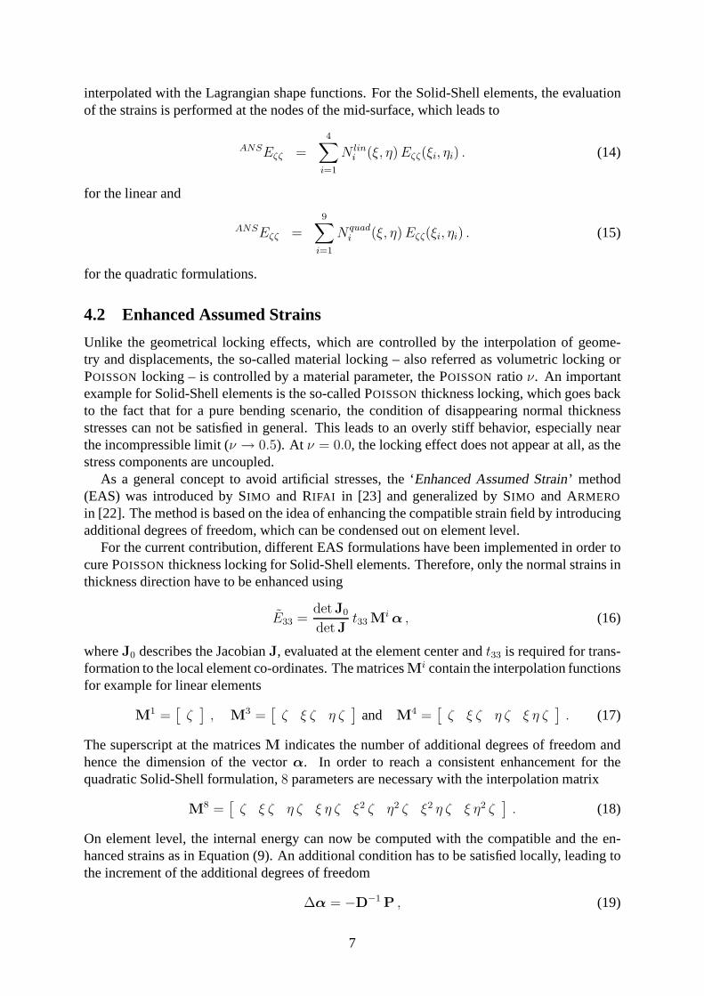
interpolated with the Lagrangian shape functions. For the Solid-Shell elements, the evaluationof the strains is performed at the nodes of the mid-surface, which leads to

ANSEζζ =

4∑

i=1

N lini (ξ, η) Eζζ(ξi, ηi) . (14)

for the linear and

ANSEζζ =9∑

i=1

N quadi (ξ, η) Eζζ(ξi, ηi) . (15)

for the quadratic formulations.

4.2 Enhanced Assumed Strains

Unlike the geometrical locking effects, which are controlled by the interpolation of geome-try and displacements, the so-called material locking – also referred as volumetric locking orPOISSON locking – is controlled by a material parameter, the POISSON ratio ν. An importantexample for Solid-Shell elements is the so-called POISSON thickness locking, which goes backto the fact that for a pure bending scenario, the condition ofdisappearing normal thicknessstresses can not be satisfied in general. This leads to an overly stiff behavior, especially nearthe incompressible limit (ν → 0.5). At ν = 0.0, the locking effect does not appear at all, as thestress components are uncoupled.

As a general concept to avoid artificial stresses, the ‘Enhanced Assumed Strain’ method(EAS) was introduced by SIMO and RIFAI in [23] and generalized by SIMO and ARMERO

in [22]. The method is based on the idea of enhancing the compatible strain field by introducingadditional degrees of freedom, which can be condensed out onelement level.

For the current contribution, different EAS formulations have been implemented in order tocure POISSONthickness locking for Solid-Shell elements. Therefore, only the normal strains inthickness direction have to be enhanced using

E33 =detJ0

detJt33 M

i α , (16)

whereJ0 describes the JacobianJ, evaluated at the element center andt33 is required for trans-formation to the local element co-ordinates. The matricesM

i contain the interpolation functionsfor example for linear elements

M1 =

[

ζ]

, M3 =

[

ζ ξ ζ η ζ]

and M4 =

[

ζ ξ ζ η ζ ξ η ζ]

. (17)

The superscript at the matricesM indicates the number of additional degrees of freedom andhence the dimension of the vectorα. In order to reach a consistent enhancement for thequadratic Solid-Shell formulation,8 parameters are necessary with the interpolation matrix

M8 =

[

ζ ξ ζ η ζ ξ η ζ ξ2 ζ η2 ζ ξ2 η ζ ξ η2 ζ]

. (18)

On element level, the internal energy can now be computed with the compatible and the en-hanced strains as in Equation (9). An additional condition has to be satisfied locally, leading tothe increment of the additional degrees of freedom

∆α = −D−1

P , (19)

7

with the matrices

P = Πint,α and D = Πint

,αα(20)

as derivatives of the internal energy with respect to the additional degrees of freedom.As can be seen in Equation (19), the matrixD from Equation (20) has to be inverted on ele-

ment level. The dimension of this square matrix is equal to the number of EAS parameters, thusthe numerical effort of the EAS elements is strongly affected by the number of enhancements.

5 Implementation Concept

Compared to implicit time integration algorithms, which are dominated by the solution of equa-tions, the central difference scheme as an explicit time integration method requires far less op-erations on global level. As discussed in Section 2, only vector operations have to be performedon global level. This and the already mentioned very small time steps lead to the fact that –within an explicit time integration scheme – most of the time, necessary for an entire structuralanalysis, is spent on element level. In different examples,computed with the in-house finiteelement code FEAP-MEKA [21], based on FEAP by R.L. TAYLOR, up to – or even more than– 90 % of the overall CPU-time had been spent on element level. For commercial codes, thisfracture may be smaller, due to computationally expensive procedures on global level whichare not yet implemented in the explicit version of the used academic code, e. g. contact searchalgorithms. Nevertheless it is obvious, that the element processing requires a dominant part ofthe overall simulation time, which motivates an efficient implementation of element code.

5.1 AceGen

In order to achieve an efficient and comfortable implementation of the subroutines on elementlevel, the improved – so-called ’automatic’ – code generation and optimization tool ACEGEN,a plug-in for the computer algebra software MATHEMATICA is used. The program is devel-oped by the group of KORELC, see [13, 16, 14]. The plug-in uses the symbolic capabilitiesof MATHEMATICA in order to create automatically optimized program code in FORTRAN. Itis possible to enter formulas as written, without botheringabout programming issues. Hencematrix operations, summations, differentiation – also with respect to vectors and matrices – canbe implemented straight forward and programming errors canbe reduced significantly.

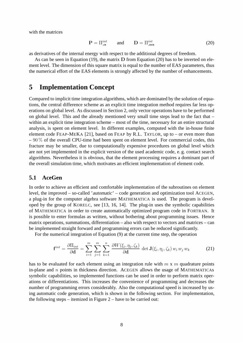
For the numerical integration of Equation (9) at the currenttime step, the operation

fint =

∂Πint

∂d=

m∑

i=1

m∑

j=1

n∑

k=1

∂W (ξi, ηj, ζk)

∂ddetJ(ξi, ηj , ζk) wi wj wk (21)

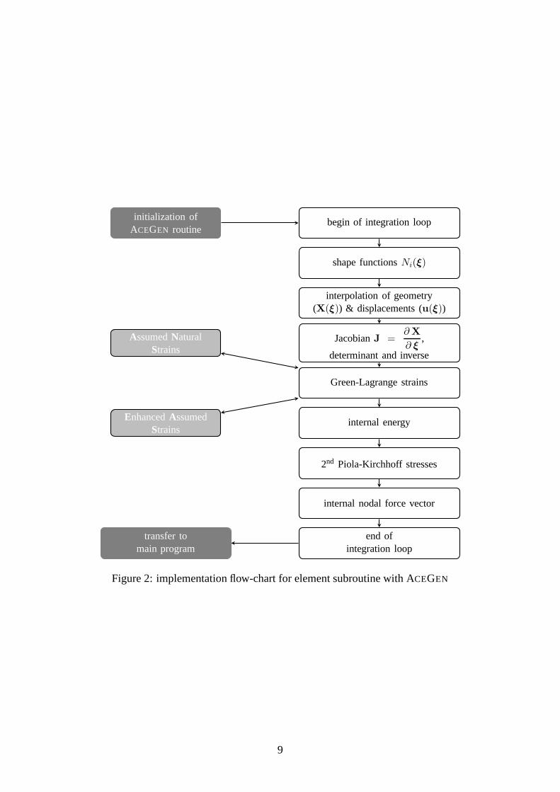
has to be evaluated for each element using an integration rule with m x m quadrature pointsin-plane andn points in thickness direction. ACEGEN allows the usage of MATHEMATICA ssymbolic capabilities, so implemented functions can be used in order to perform matrix oper-ations or differentiations. This increases the convenience of programming and decreases thenumber of programming errors considerably. Also the computational speed is increased by us-ing automatic code generation, which is shown in the following section. For implementation,the following steps – itemized in Figure 2 – have to be carriedout:

8

initialization ofACEGEN routine

begin of integration loop

shape functionsNi(ξ)

interpolation of geometry(X(ξ)) & displacements (u(ξ))

JacobianJ =∂ X

∂ ξ,

determinant and inverse

Green-Lagrange strains

internal energy

2nd Piola-Kirchhoff stresses

internal nodal force vector

end ofintegration loop

transfer tomain program

AssumedNaturalStrains

EnhancedAssumedStrains

Figure 2: implementation flow-chart for element subroutinewith ACEGEN

9

Initialization: The subroutine as well as the input (geometry, current displacements, coor-dinates and weights of the quadrature points and material parameters) and output variables(internal force vector) are defined. The used ACEGEN commands areSMSInitialize andSMSModule.

Element matrices: After the import of the element data, the necessary matricesand vectors –Jacobian, convective base vectors, Green-Lagrange straintensor, etc. – can be evaluated usingMATHEMATICA ’s symbolic capabilities. Differentiation with respect tovariables or tensors isalso possible (SMSD), which is used e. g. to evaluateΠint

,d .

Export internal force vector: The internal force vector at the current integration point hasto be exported, to be available outside the symbolic subroutine. The commandSMSExport isused with the option"AddIn"=True in order to automatically sum the results for all quadra-ture points to the global memory field.

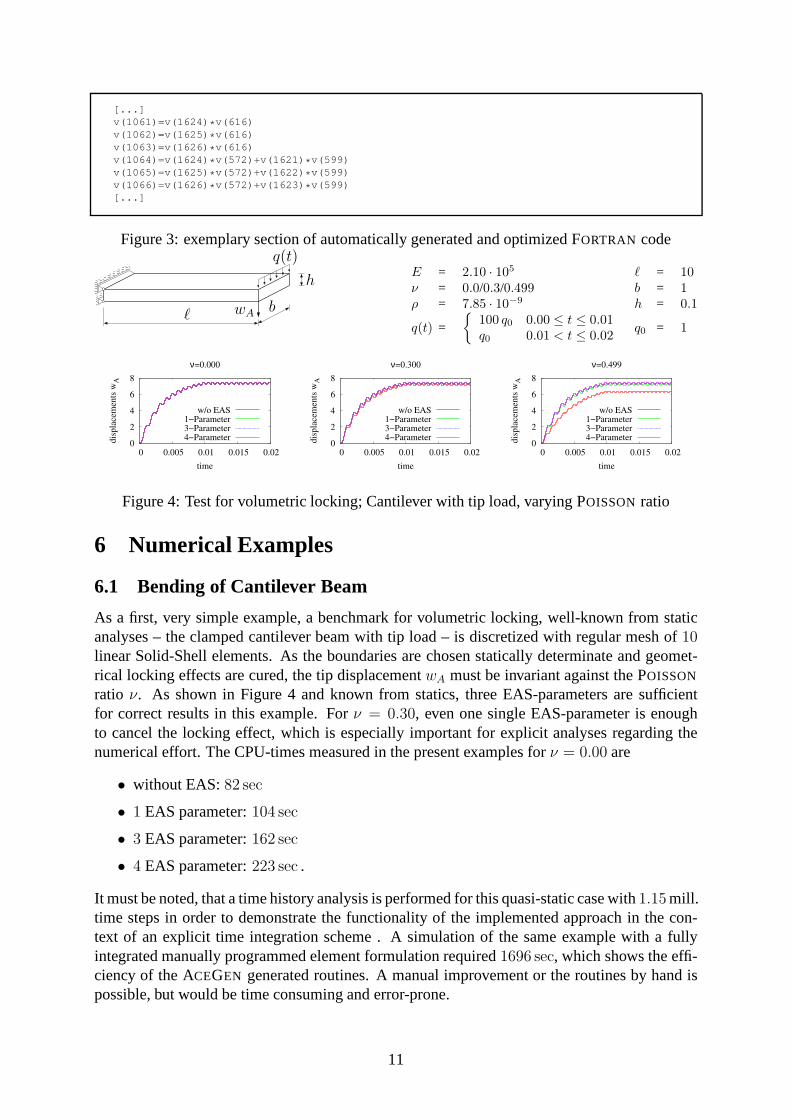
Code generation: In the last step, FORTRAN-code is generated and automatically optimized,using the commandSMSWrite. The language (FORTRAN, C, etc.) and the level of opti-mization depend on options, defined inSMSInitialize. Figure 3 shows a portion of thisautomatically generated FORTRAN-code.

The efficiency and performance of the automatically generated and simultaneously optimizedsubroutines is coupled to some conditions and rules, one hasto consider when using the pro-gramming tool. The main challenge is to reach a consequent application of the symbolic capa-bilities. It is important to identify the numerically ‘expensive’ operations within an algorithmand concentrate them into as few as possible routines. The subdivision of a procedure intomany small routines as it is usually done in manual programming is not optimal here, as thesymbolically used variables have to be initialized every time. In the present case, all operationsnecessary for the computation of the internal forces are performed in a single routine as shownsymbolically in Figure 2. Consequently, ACEGEN is able to optimize the generated code withregard to the performed operations and produce highly efficient code. Compared to manualprogramming, the initialization and introduction of variables as well as the transfer of data intoand out of the subroutine is the main difficulty when using ACEGEN. Another problem is thedebugging, as the generated code is not longer readable – as can be seen in Figure 3. Furtherany change in the program requires a complete re-generationof the subroutine with ACEGEN.Errors in the initialization of variables can lead to wrong results when performing e. g. symbolicdifferentiations. This errors can only be found and corrected using MATHEMATICA , as manualdebugging is not possible.

The correct application of ACEGEN – which required some learning time and gaining ofexperience – allows the direct implementation of symbolic algorithms and the fast and error-free generation of program code. Also modification in the element formulation can be imple-mented without programming errors. The generated code is highly efficient, as can be seen inthe following numerical examples. As the contrast an improvement of manually implementedroutines in order to achieve a significant speed-up is exhausting and error-prone and hencetime-consuming.

10

[...]v(1061)=v(1624)*v(616)v(1062)=v(1625)*v(616)v(1063)=v(1626)*v(616)v(1064)=v(1624)*v(572)+v(1621)*v(599)v(1065)=v(1625)*v(572)+v(1622)*v(599)v(1066)=v(1626)*v(572)+v(1623)*v(599)[...]

Figure 3: exemplary section of automatically generated andoptimized FORTRAN code

ℓ wA b

h

q(t)E = 2.10 · 105 ℓ = 10ν = 0.0/0.3/0.499 b = 1ρ = 7.85 · 10−9 h = 0.1

q(t) =

{

100 q0 0.00 ≤ t ≤ 0.01q0 0.01 < t ≤ 0.02

q0 = 1

0

2

4

6

8

0 0.005 0.01 0.015 0.02

dis

pla

cem

ents

wA

time

ν=0.000

w/o EAS1−Parameter3−Parameter4−Parameter

0

2

4

6

8

0 0.005 0.01 0.015 0.02

dis

pla

cem

ents

wA

time

ν=0.300

w/o EAS1−Parameter3−Parameter4−Parameter

0

2

4

6

8

0 0.005 0.01 0.015 0.02

dis

pla

cem

ents

wA

time

ν=0.499

w/o EAS1−Parameter3−Parameter4−Parameter

Figure 4: Test for volumetric locking; Cantilever with tip load, varying POISSON ratio

6 Numerical Examples

6.1 Bending of Cantilever Beam

As a first, very simple example, a benchmark for volumetric locking, well-known from staticanalyses – the clamped cantilever beam with tip load – is discretized with regular mesh of10linear Solid-Shell elements. As the boundaries are chosen statically determinate and geomet-rical locking effects are cured, the tip displacementwA must be invariant against the POISSON

ratio ν. As shown in Figure 4 and known from statics, three EAS-parameters are sufficientfor correct results in this example. Forν = 0.30, even one single EAS-parameter is enoughto cancel the locking effect, which is especially importantfor explicit analyses regarding thenumerical effort. The CPU-times measured in the present examples forν = 0.00 are

• without EAS:82 sec

• 1 EAS parameter:104 sec

• 3 EAS parameter:162 sec

• 4 EAS parameter:223 sec .

It must be noted, that a time history analysis is performed for this quasi-static case with1.15 mill.time steps in order to demonstrate the functionality of the implemented approach in the con-text of an explicit time integration scheme . A simulation ofthe same example with a fullyintegrated manually programmed element formulation required1696 sec, which shows the effi-ciency of the ACEGEN generated routines. A manual improvement or the routines byhand ispossible, but would be time consuming and error-prone.

11

free boundarywith verticallyprescribeddisplacement

free boundarywith verticallyprescribeddisplacement

PP ��

ℓ

r

t

d

0.0

∆1

∆2

0.0 0.10 0.15

[dis

pla

cem

ent]

[time]

E = 210 · 109

ν = 0.3ρ = 7.85 · 10−9

ℓ = 2t = 0.02r = 0.25d = 0.01

∆1 = 0.5∆2 = 0.9

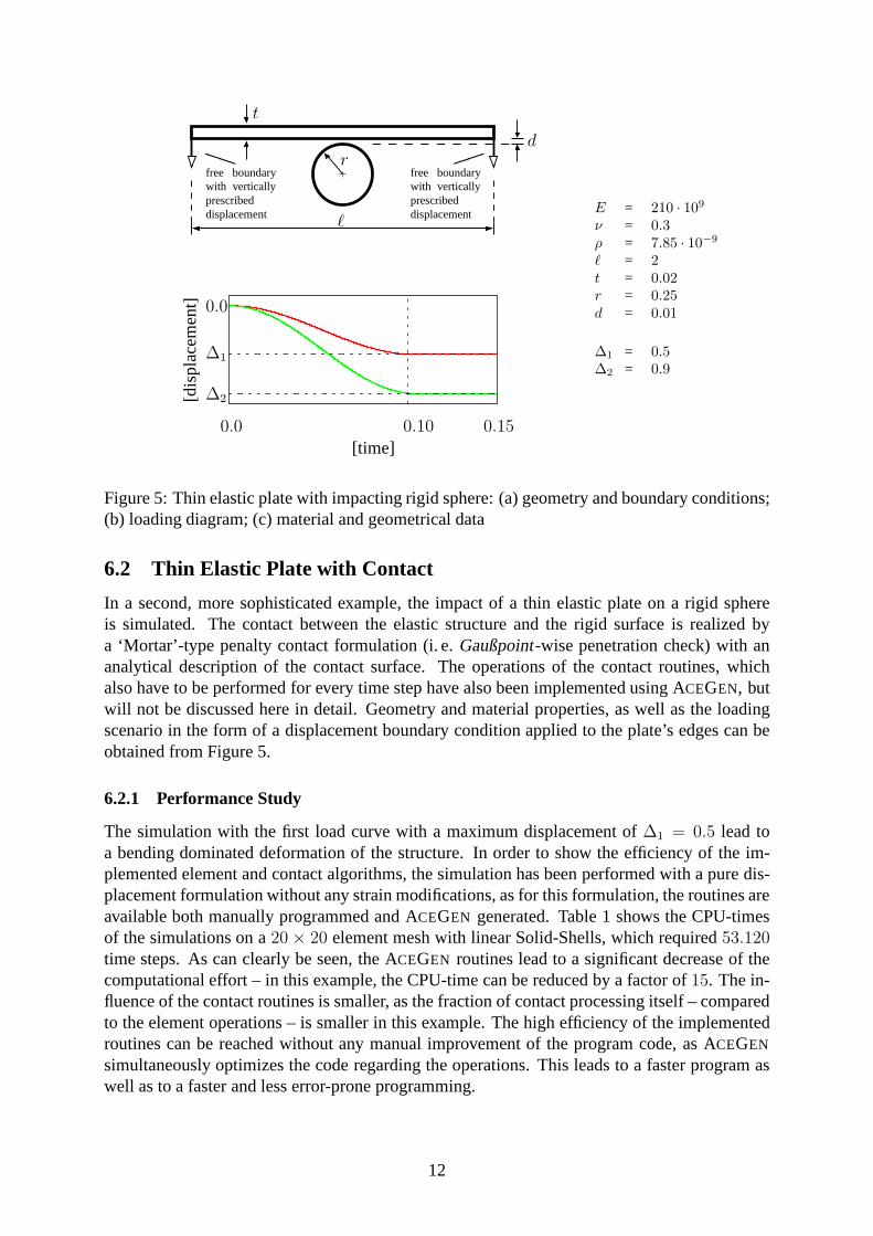
Figure 5: Thin elastic plate with impacting rigid sphere: (a) geometry and boundary conditions;(b) loading diagram; (c) material and geometrical data

6.2 Thin Elastic Plate with Contact

In a second, more sophisticated example, the impact of a thinelastic plate on a rigid sphereis simulated. The contact between the elastic structure andthe rigid surface is realized bya ‘Mortar’-type penalty contact formulation (i. e.Gaußpoint-wise penetration check) with ananalytical description of the contact surface. The operations of the contact routines, whichalso have to be performed for every time step have also been implemented using ACEGEN, butwill not be discussed here in detail. Geometry and material properties, as well as the loadingscenario in the form of a displacement boundary condition applied to the plate’s edges can beobtained from Figure 5.

6.2.1 Performance Study

The simulation with the first load curve with a maximum displacement of∆1 = 0.5 lead toa bending dominated deformation of the structure. In order to show the efficiency of the im-plemented element and contact algorithms, the simulation has been performed with a pure dis-placement formulation without any strain modifications, asfor this formulation, the routines areavailable both manually programmed and ACEGEN generated. Table 1 shows the CPU-timesof the simulations on a20 × 20 element mesh with linear Solid-Shells, which required53.120time steps. As can clearly be seen, the ACEGEN routines lead to a significant decrease of thecomputational effort – in this example, the CPU-time can be reduced by a factor of15. The in-fluence of the contact routines is smaller, as the fraction ofcontact processing itself – comparedto the element operations – is smaller in this example. The high efficiency of the implementedroutines can be reached without any manual improvement of the program code, as ACEGEN

simultaneously optimizes the code regarding the operations. This leads to a faster program aswell as to a faster and less error-prone programming.

12

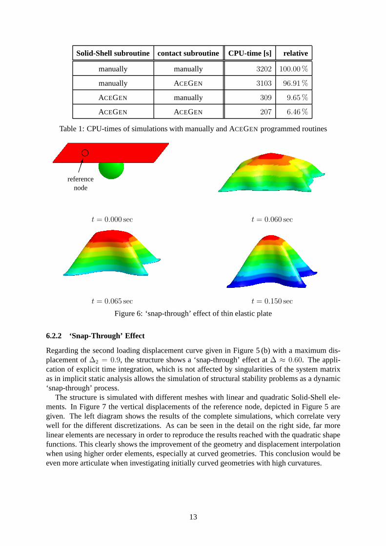
Solid-Shell subroutine contact subroutine CPU-time [s] relative

manually manually 3202 100.00 %

manually ACEGEN 3103 96.91 %

ACEGEN manually 309 9.65 %

ACEGEN ACEGEN 207 6.46 %

Table 1: CPU-times of simulations with manually and ACEGEN programmed routines

t = 0.000 sec

t = 0.065 sec

t = 0.060 sec

t = 0.150 sec

referencenode

i����

Figure 6: ‘snap-through’ effect of thin elastic plate

6.2.2 ‘Snap-Through’ Effect

Regarding the second loading displacement curve given in Figure 5 (b) with a maximum dis-placement of∆2 = 0.9, the structure shows a ‘snap-through’ effect at∆ ≈ 0.60. The appli-cation of explicit time integration, which is not affected by singularities of the system matrixas in implicit static analysis allows the simulation of structural stability problems as a dynamic‘snap-through’ process.

The structure is simulated with different meshes with linear and quadratic Solid-Shell ele-ments. In Figure 7 the vertical displacements of the reference node, depicted in Figure 5 aregiven. The left diagram shows the results of the complete simulations, which correlate verywell for the different discretizations. As can be seen in thedetail on the right side, far morelinear elements are necessary in order to reproduce the results reached with the quadratic shapefunctions. This clearly shows the improvement of the geometry and displacement interpolationwhen using higher order elements, especially at curved geometries. This conclusion would beeven more articulate when investigating initially curved geometries with high curvatures.

13

−0.50

−0.40

−0.30

−0.20

−0.10

0.00

0 0.03 0.06 0.09 0.12 0.15

z−d

isp

lace

men

t

time

20x20 quad40x40 lin80x80 lin

160x160 lin

(a) displacement of reference node

−0.30

−0.20

−0.10

0.06 0.0625 0.065

z−d

isp

lace

men

t

time

20x20 quad40x40 lin80x80 lin

160x160 lin

(b) detail with ‘snap-through’

����

detail-

Figure 7: results of different discretizations with linearand quadratic Solid-Shells

7 Conclusions & Outlook

In the paper Solid-Shell element formulations with linear and quadratic interpolation of thein-plane geometry and displacement withAssumed Natural Strainsand Enhanced AssumedStrainsin order to reduce artificial stiffness effects are presented. An implementation conceptusing the automatic code generation tool ACEGEN based on the computer algebra programMATHEMATICA is shown and the advantages regarding programming and computational effi-ciency are discussed. Especially in the context of explicittime integration, efficient elementroutines are very important, as the fracture of element processing on the overall simulation timeis extremely high. The numerical examples show the improvement of the ACEGEN generatedelement routines compared to a manually performed implementation.

In the course of the project, the application of ACEGEN for further element formulationsis planned, also structural elements (i. e. shell elements)with linear and quadratic geometryand displacement interpolations are currently implemented, as they are especially importantfor applications with explicit time integration. As a very positive result we can conclude thatthe use of symbolic programming seems to be advantageous in many applications in structuralmechanics. A very promising application is the implementation of complex material models, ashere the advantage of automatic differentiation is particularly interesting.

Acknowledgements

The presented work is part of a project, currently funded by the German Research Foundation(DFG). The support is gratefully acknowledged.

References

[1] R.J. Alves de Sousa, R.P.R. Cardoso, R.A. Fontes Valente, J.W. Yoon, R.M. Natal Jorge,and J.J. Gracio. A new one-point quadrature enhanced assumed strain (EAS) solid-shellelement with multiple integration points along thickness:Part I – geometrically linearapplications.Int. J. Num. Meth. Eng., 62:952–977, 2005.

14

[2] K.-J. Bathe and E.N. Dvorkin. A formulation of general shell elements - the use of mixedinterpolation of tensorial components.International Journal For Numerical Methods InEngineering, 22:697–722, 1986.

[3] T. Belytschko, W.K. Liu, and B. Moran.Nonlinear finite elements for continua and struc-tures. Wiley, 2004.

[4] P. Betsch and E. Stein. An assumed strain approach avoiding artifical thickness strain-ing for an non-linear 4-node shell element.Communications In Numerical Methods InEngineering, 11:899–909, 1995.

[5] M. Bischoff and E. Ramm. Shear deformable shell elementsfor large strains and rotations.International Journal For Numerical Methods In Engineering, 40:4427–4449, 1997.

[6] M.L. Bucalem and K.-J. Bathe. Higher-order mitc generalshell elements.InternationalJournal For Numerical Methods In Engineering, 36(21):3729–3754, 1993.

[7] R.P.R. Cardoso, J.W. Yoon, M. Mahardika, S. Choudhry, R.J. Alves de Sousa, and R.A.Fontes Valente. Enhanced assumed strain (eas) and assumed natural strain (ans) meth-ods for one-point quadrature solid-shell elements.International Journal For NumericalMethods In Engineering, 75:156–187, 2008.

[8] R. Courant, K.O. Friedrichs, and H. Lewy.Uber die partiellen Differenzengleichungender mathematischen Physik.Mathematische Annalen, 100:32–74, 1928.

[9] M. Harnau, K. Schweizerhof, and R.Hauptmann. On ’solid-shell’ elements with linearand quadratic shape functions for small and large deformations. ECCOMAS Congress,11, 2000.

[10] R. Hauptmann, S. Doll, M. Harnau, and K. Schweizerhof. ‘solid-shell’ elements withlinear and quadratic shape functions at large deformationswith nearly incompressible ma-terials.Computers & Structures, 79(18):1671–1685, 2001.

[11] R. Hauptmann and K. Schweizerhof. A systematic development of ‘solid-shell’ elementformulations for linear and non-linear analyses employingonly displacement degrees offreedom.Int. J. Num. Meth. Eng., 42(1):49–69, 1998.

[12] Thomas J. R. Hughes.The finite element method. Dover Publ., dover ed., 1. publ. edition,2000.

[13] J. Korelc. Automatic generation of finite-element codeby simultaneous optimization ofexpressions.Theoretical Computer Science, 187(1-2):231–248, 1997.

[14] J. Korelc. Multi-language and multi-environment generation of nonlinear finite elementcodes.Engineering with Computers, 18(4):312–327, 2002.

[15] J. Korelc.http://www.fgg.uni-lj.si/Symech/, 2010.

[16] J. Korelc and P. Wriggers. Computer algebra and automatic differentiation in derivationof finite element code.ZAMM, 79:811–812, 1999.

[17] C. Miehe. A theoretical and computational model for isotropic elastoplastic stress analysisin shells at large strains.Comput. Meth. Appl. Mech. Eng., 155(3-4):193–234, 1998.

15

[18] H. Parisch. A continuum-based shell theory for non-linear applications.Int. J. Num. Meth.Eng., 38:1855–1883, 1995.

[19] S. Reese. A large deformation solid-shell concept based on reduced integration with hour-glass stabilization.Int. J. Num. Meth. Eng., 69(8):1671–1716, 2007.

[20] M. Schwarze and S. Reese. A reduced integration solid-shell finite element based onthe eas and the ans concept - geometrically linear problems.International Journal forNumerical Methods in Engineering, 80(10):1322–1355, 2009.

[21] K. Schweizerhof and Coworkers. Feap-meka, finite element analysis program. KarlsruherInstitut fur Technologie, based on Version 1994 of R. Taylor, “FEAP – A Finite ElementAnalysis Program”, University of California, Berkeley.

[22] J.C. Simo and F. Armero. Geometrically non-linear enhanced strain mixed methods andthe method of incompatible modes.International Journal For Numerical Methods InEngineering, 33:1413–1449, 1992.

[23] J.C. Simo and M.S. Rifai. A class of mixed assumed strainmethods and the method ofincompatible modes.Computers & Structures, 29:1595–1638, 1990.

[24] L. Verlet. ‘Experiments’ on classical fluids I. Thermomechanical properties of Lennard-Jones molecules.Physical Review, 159:98–103, 1967.

16