Information Measures of Complexity, Emergence,Self-organization, Homeostasis, and Autopoiesis

Nelson Fernandez1,2, Carlos Maldonado3,4 & Carlos Gershenson4,5

1 Laboratorio de Hidroinformatica, Facultad de Ciencias BasicasUnivesidad de Pamplona, Colombia

http://unipamplona.academia.edu/NelsonFernandez2 Centro de Micro-electronica y Sistemas Distribuidos,

Universidad de los Andes, Merida, Venezuela3 Facultad de Ciencias

Universidad Nacional Autonoma de Mexico4 Departamento de Ciencias de la Computacion

Instituto de Investigaciones en Matematicas Aplicadas y en SistemasUniversidad Nacional Autonoma de Mexico

5 Centro de Ciencias de la ComplejidadUniversidad Nacional Autonoma de Mexico

cgg@unam.mx http://turing.iimas.unam.mx/˜cgg

August 1, 2013

Abstract

This chapter reviews measures of emergence, self-organization, complexity, home-ostasis, and autopoiesis based on information theory. These measures are derived fromproposed axioms and tested in two case studies: random Boolean networks and anArctic lake ecosystem.

Emergence is defined as the information a system or process produces. Self-organizationis defined as the opposite of emergence, while complexity is defined as the balance be-tween emergence and self-organization. Homeostasis reflects the stability of a system.Autopoiesis is defined as the ratio between the complexity of a system and the com-plexity of its environment. The proposed measures can be applied at different scales,which can be studied with multi-scale profiles.

1 IntroductionIn recent decades, the scientific study of complex systems (Bar-Yam, 1997; Mitchell, 2009)has demanded a paradigm shift in our worldviews (Gershenson et al., 2007; Heylighen et al.,

1

arX

iv:1

304.

1842

v3 [

nlin

.AO

] 3

1 Ju

l 201

3

2007). Traditionally, science has been reductionistic. Still, complexity occurs when compo-nents are difficult to separate, due to relevant interactions. These interactions are relevantbecause they generate novel information which determines the future of systems. This facthas several implications (Gershenson, 2013). A key implication: reductionism—the mostpopular approach in science—is not appropriate for studying complex systems, as it attemptsto simplify and separate in order to predict. Novel information generated by interactionslimits prediction, as it is not included in initial or boundary conditions. It implies compu-tational irreducibility (Wolfram, 2002), i.e. one has to reach a certain state before knowingit will be reached. In other words, a priori assumptions are of limited use, since the precisefuture of complex systems is known only a posteriori. This does not imply that the futureis random, it just implies that the degree to which the future can be predicted is inherentlylimited.

It can be said that this novel information is emergent, since it is not in the components,but produced by their interactions. Interactions can also be used by components to self-organize, i.e. produce a global pattern from local dynamics. Interactions are also key forfeedback control loops, which help systems regulate their internal states, an essential aspectof living systems.

We can see that reductionism is limited for describing such concepts as complexity, emer-gence, self-organization, and life. In the wake of the fall of reductionism as a dominant world-view (Morin, 2007), a plethora of definitions, notions, and measures of these concepts hasbeen proposed. Still, their diversity seems to have created more confusion than knowledge.In this chapter, we revise a proposal to ground measures of these concepts in informationtheory. This approach has several advantages:• Measures are precise and formal.

• Measures are simple enough to be used and understood by people without a strongmathematical background.

• Measures can help clarify the meaning of the concepts they describe.

• Measures can be applied to any phenomenon, as anything can be described in termsof information (Gershenson, 2012b).

This chapter is organized as follows: In the next section, background concepts are pre-sented, covering briefly complexity, emergence, self-organization, homeostasis, autopoiesis,information theory, random Boolean networks, and limnology. Section 3 presents axioms andderives measures for emergence, self-organization, complexity, homeostasis and autopoiesis.To illustrate the measures, these are applied to two case studies in Section 4: random Booleannetworks and an Arctic lake ecosystem. Discussion and conclusions close the chapter.

2 Background

2.1 ComplexityThere are dozens of notions and measures of complexity, proposed in different areas withdifferent purposes (Edmonds, 1999; Lloyd, 2001). Etymologically, complexity comes from

2

the Latin plexus, which means interwoven. Thus, something complex is difficult to separate.This means that its components are interdependent, i.e. their future is partly determinedby their interactions (Gershenson, 2013). Thus, studying the components in isolation—asreductionistic approaches attempt—is not sufficient to describe the dynamics of complexsystems.

Nevertheless, it would be useful to have global measures of complexity, just as tempera-ture characterizes the properties of kinetic energy of molecules or photons. Each componentcan have a different kinetic energy, but the statistical average is represented in the temper-ature. For complex systems, particular interactions between components can be different,but we can say that complexity measures should represent the type of interactions betweencomponents, just as Lyapunov exponents characterize different dynamical regimes.

A useful measure of complexity should enable us to answer questions such as: Is a desertmore or less complex than a tundra? What is the complexity of different influenza outbreaks?Which organisms are more complex: predators or preys; parasites or hosts; individual orsocial? What is the complexity of different music genres? What is the required complexityof a company to face the complexity of a market1?

Moreover, with the recent scandalous increase of data availability in most domains, weurgently need measures to make sense of it.

2.2 EmergenceEmergence has probably been one of the most misused concepts in recent decades. Thereasons for this misuse are varied and include: polysemy (multiple meanings), buzzwording,confusion, hand waving, Platonism, and even mysticism. Still, the concept of emergencecan be clearly defined and understood (Anderson, 1972). The properties of a system areemergent if they are not present in their components. In other words, global propertieswhich are produced by local interactions are emergent. For example, the temperature of agas can be said to be emergent (Shalizi, 2001), since the molecules do not possess such aproperty: it is a property of the collective. In a broad an informal way, emergence can beseen as differences in phenomena as they are observed at different scales (Prokopenko et al.,2009).

Some might perceive difficulties in describing phenomena at different scales (Gershenson,2013), but this is a consequence of attempting to find a single “true” description of phe-nomena. Phenomena do not depend on the descriptions we have of them, and we can haveseveral different descriptions of the same phenomenon. It is more informative to handle sev-eral descriptions at once, and actually it is necessary when studying emergence and complexsystems.

2.3 Self-organizationSelf-organization has been used to describe swarms, flocks, traffic, and many other systemswhere the local interactions lead to a global pattern or behavior (Camazine et al., 2003;Gershenson, 2007). Intuitively, self-organization implies that a system increases its own

1This question is related to the law of requisite variety (Ashby, 1956).

3

organization. This leads to the problems of defining organization, system, and self. Moreover,as Ashby showed (1947b), almost any dynamical system can be seen as self-organizing: if ithas an attractor, and we decide to call that attractor “organized”, then the system dynamicswill tend to it, thus increasing by itself its own organization. If we can describe almost anysystem as self-organizing, the question is not whether a system is self-organizing or not, butrather, when is it useful to describe a system as self-organizing (Gershenson and Heylighen,2003)?

In any case, it is convenient to have a measure of self-organization which can capture thenature of local dynamics at a global scale. This is especially relevant for the nascent fieldof guided self-organization (GSO) (Prokopenko, 2009; Ay et al., 2012; Polani et al., 2013).GSO can be described as the steering of the self-organizing dynamics of a system towardsa desired configuration (Gershenson, 2012a). This desired configuration will not always bethe natural attractor of a controlled system. The mechanisms for guiding the dynamics andthe design of such mechanisms will benefit from measures characterizing the dynamics ofsystems in a precise and concise way.

2.4 HomeostasisOriginally, the concept of homeostasis was developed to describe internal and physiologicalregulation of bodily functions, such as temperature or glucose levels. Probably the firstperson to recognize the internal maintenance of a near-constant environment as a conditionfor life was Bernard (1859). Subsequently, Canon (1932) coined the term homeostasis fromthe Greek homoios (similar) and stasis (standing still). Cannon defined homeostasis as theability of an organism to maintain steady states of operation during internal and externalchanges. Homeostasis does not imply an immobile or a stagnant state. Although someconditions may vary, the main properties of an organism are maintained.

Later, the British cybernetician William R. Ashby proposed, in an alternative form,that homeostasis implicates an adaptive reaction to maintain “essential variables” within arange (Ashby, 1947a, 1960). In order to explain the generation of behavior and learning inmachines and living systems, Ashby also contributed by linking the concepts of ultrastabilityand homeostatic adaptation (Di Paolo, 2000). Ultrastability refers to the normal operationof the system within a “viability zone” to deal with environmental changes. This viabilityzone is defined by the lower and upper bounds of the essential variables. If the value ofvariables crosses the limits of its viability zone, the system has a chance of finding newparameters that make the challenged variables return to their viability zone.

A dynamical system has a high homeostatic capacity if it is able to maintain its dynamicsclose to a certain state or states (attractors). As explained above, when perturbations orenvironmental changes occur, the system adapts to face the changes within the viabilityzone, that is, without the system “breaking” (Ashby, 1947a). Homeostasis can be seen asa dynamic process of self-regulation and adaptation by which systems adapt their behaviorover time (Williams, 2006). The homeostasis concept can be applied to different fields beyondlife sciences and is also closely related to self-organization and to robustness (Wagner, 2005;Jen, 2005).

4

2.5 AutopoiesisAutopoiesis comes from the Greek auto (self) and poiesis (creation, production) and wasproposed as a concept to define the living. According to Maturana (2011), the notion ofautopoiesis was created to connote and describe the molecular processes taking place inthe realization of living beings as autonomous entities. However, this meaning of the wordautopoiesis, which was used to describe closed networks of molecular production, was chosenonly until 1970 (Maturana and Varela, 1980). This notion arises from a series of questions,related to the internal dynamics of living systems, which Maturana began considering inthe 1960s, such as: “What should be the constitution of a system so that I see a livingsystem as a result of its operation?”, “What kind of systems or entities are living systems?”,and another question that a student asked Maturana: “What happened three billion eighthundred million years ago so that you can now say that living systems began then?”

In the context of autopoiesis, living beings occur as discrete autonomous dynamic molecu-lar autopoietic entities. These entities are in a continuous realization of their self-production.Thus, autopoiesis describes the internal dynamics of a living system in the molecular domain.Maturana notices that living beings are dynamical systems in continuous change. Interac-tions between elements of an autopoietic system regulate the production and regeneration ofthe system’s components, having the potential to develop, preserve, and produce their ownorganization (Varela et al., 1974).

For example, a bacterium may produce another bacterium by cellular division, while avirus requires a host cell to produce another virus. The production of the new bacteriumis made by the interactions between the elements of another bacterium. The productionof a new virus depends on interactions between elements of an external system. Thus, itcan be said that a bacterium is more autopoietic than a virus. In this sense, autopoiesis ismuch related to autonomy (Ruiz-Mirazo and Moreno, 2004). Autonomy is always limited inopen systems, as their states depend on environmental interactions. However, differences inautonomy can be clearly identified, just like in the previous example.

The concept of autopoiesis has been extended to other areas beyond biology (Luisi, 2003;Seidl, 2004; Froese and Stewart, 2010), although no formal measure had been proposed sofar.

2.6 Information TheoryInformation has had a most interesting history (Gleick, 2011). Information theory wascreated by Claude Shannon in 1948 in the context of telecommunications. He analyzedwhether it was possible to reconstruct data transmitted across a noisy channel. In hismodel, information is represented as a string X = x0x1... where each xi is a symbol froma finite set of symbols A called the alphabet. Moreover, each symbol in the alphabet hasa given probability P (x) of occurring in the string. Common symbols will have a high P (x)while infrequent symbols will have a low P (x).

Shannon was interested in a function to measure how much information a process “pro-duces”. Quoting Shannon (1948)2:

2We replaced Shannon’s H for I.

5

Suppose we have a set of possible events whose probabilities of occurrence arep1, p2, ..., pn. These probabilities are known but that is all we know about theevent that might occur. Can we find a measure of how much “choice” is involvedin the selection of the event or how uncertain we are of the outcome? If there issuch a measure, say (p1, p2, ..., pn) it is reasonable to require of it the followingproperties:

1. I should be continuous in each pi.2. If all the pi are equal, pi = 1/n, then I should be a monotonic increas-

ing function of n. With equally n likely events there is more choice, oruncertainty, when there are more possible events.

3. If a choice be broken down into two successive choices, the original I shouldbe the weighted sum of the individual values of I.

With these few axioms, Shannon demonstrates that the only function I satisfying the threeabove is of the form:

I = −Kn∑

i=i

pi log pi, (1)

where K is a positive constant.For example, if we have a string ‘0001000100010001...’, we can estimate P (0) = 0.75 and

P (1) = 0.25, then I = −(0.75 · log 0.75 + 0.25 · log 0.25). If we use K = 1 and a base 2logarithm, then I ≈ 0.811.

Shannon used H to describe information (we are using I) because he was thinking in theBoltzmann’s H theorem3 when he developed the theory. Therefore, he called equation 1 theentropy of the set of probabilities p1, p2, ..., pn. In modern words, I is a function of a randomvariable X.

The unit of information is the bit (binary digit). One bit represents the informationgained when a binary random variable becomes known. However, since equation 1 is a sumof probabilities, Shannon’s information is a unitless measure.

More details about information theory in general can be found in Ash (1990), whilea primer on information theory related to complexity, self-organization, and emergence isfound in Prokopenko et al. (2009).

2.7 Random Boolean NetworksRandom Boolean networks (RBNs) are abstract computational models, originally proposedto study genetic regulatory networks (Kauffman, 1969, 1993). However, being general mod-els, their study and use has expanded beyond biology (Aldana-Gonzalez et al., 2003; Ger-shenson, 2004, 2012a).

A RBN is formed by N nodes linked by K connections4. Each node has a Boolean state,i.e. zero or one. The future state of each node is determined by the current states of the

3The Boltzmann H theorem is given in the thermodinamic context. It states that the entropy of an idealgas increases in an irreversible process. This might be also the reason why he required the second property.

4This K is different from the constant used in equation 1.

6

nodes that link to it and a lookup table which specifies how the update will take place. Theconnectivity (which nodes affect which) and the lookup tables (how nodes affect their states)are usually generated randomly for a network, but remain fixed during its dynamics.

RBNs have been found to have three different dynamical regimes, which have been studiedextensively (Gershenson, 2004):

Ordered. Most nodes are static, RBNs are robust to perturbations.

Chaotic. Most nodes are changing, RBNs are fragile to perturbations.

Critical. Some nodes are changing, RBNs have adaptive potential.

Different parameters and properties determine the regime, which can be used to guide aparticular RBN towards a desired regime (Gershenson, 2012a).

It can be said that the critical regime balances the robustness of the chaotic regime andthe changeability of the chaotic regime. It has been argued that computation and life requirethis balance to be able to compute and adapt (Langton, 1990; Kauffman, 1993).

RBNs will be used in Section 4.1 to illustrate the measures proposed in the next section.

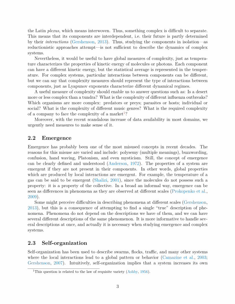
2.8 LimnologyLakes are studied by limnology. Lakes can be divided in different zones, as shown in Figure 1:(i) The macrophyte zone, composed mainly of aquatic plants, which are rooted, floating orsubmerged. (ii) The planktonic zone corresponds to the open surface waters; away fromthe shore in which organisms passively float and drift (phyto and zooplankton). Planktonicorganisms are incapable of swimming against a current. However, some of them are motile.(iii) The benthic zone is the lowest level of a body of water related with the substratum,including the sediment surface and subsurface layers. (iv) The mixing zone is where theexchange of water from planktonic and benthic zones occurs.

At different zones, one or more components or subsystems can be an assessment forthe ecosystem dynamics. For our case study to be presented in Section 4.2, we consideredthree components: physiochemical, limiting nutrients and photosynthetic biomass for theplanktonic and benthic zones.

The physiochemical component refers to the chemical composition of water. It is affectedby various conditions and processes such as geological nature, the water cycle, dispersion,dilution, solute and solids generation (e.g. photosynthesis), and sedimentation. In thiscomponent, we highlight two water variables that are important for the aquatic life: (i) thepH equilibrium that affects, among others, the interchange of elements between the organismand its environment and (ii) the temperature regulation that is supported in the specific heatof the water.

Related to the physiochemical component, limiting nutrients which are basic for photo-synthesis are associated with the biogeochemical cycles of nitrogen, carbon, and phosphorous.These cycles permit the adsorption of gases into the water or the dilution of some limitingnutrients.

In addition, among limnetic biota, photoautotrophic biomass is the basis for the trophicweb establishment. The term autotrophs is used for organisms that increase their mass

7

Surface  zone

Macrophytes zone Planktonic zone

Mixing zone

Benthic zone

Substratum

Inflow Outflow

Figure 1: Zones of lakes studied in limnology.

8

through the accumulation of proteins which they manufacture, mainly from inorganic rad-icals (Stumm, 2004). This type of organisms can be found at the planktonic and benthiczones.

The previous basic limnology concepts will be useful to follow the case study of an Arcticlake, presented in Section 4.2.

3 MeasuresWe have recently proposed earlier versions of the measures presented in this chapter (Fernandezet al., 2012; Gershenson and Fernandez, 2012). The ones presented here are more refinedand are based on axioms. The benefit of using axioms is that the discussion is not taken somuch at the level of the measures, but at the level of the presuppositions or the propertieswe want measures to have.

A comparison of the proposed measures with others can be found in Gershenson andFernandez (2012). It is worth noting that all of the proposed measures are unitless.

3.1 EmergenceWe mentioned that emergence refers to properties of a phenomenon which are present at onescale and are not at another scale. Scales can be temporal or spatial. If we describe phenom-ena in terms of information, in order to have “new” information, “old” information has tobe transformed. This transformation can be dynamic, static, active, or stigmergic (Gershen-son, 2012b). For example, new information is produced when a dynamical system changesits behavior, but also when a description of a system changes. Concerning the first case,approaches measuring the difference between past and future states have been proposed,e.g. (Shalizi and Crutchfield, 2001). We can call this dynamic emergence. Concerning thesecond case, approaches measuring differences between scales have been used, e.g. (Shal-izi, 2001; Holzer and De Meer, 2011). We can call this scale emergence. Even when thereare differences between dynamic and scale emergencies, both can be seen as new informa-tion being produced. In the first case, dynamics produce new information. In the secondcase, the change of description produces new information. Thus, information emergence Eincludes both dynamic emergence and scale emergence. If we recall, Shannon proposed aquantity which measures how much information a process “produces”. Therefore, we can saythat emergence is the same as Shannon’s information I. From now on, we will consider theemergence of a process E as the information I and we will use the base two logarithm.

E = I. (2)

We now revise that the intuitive idea of emergence fulfills the three basic notions (axioms)that Shannon used to derive I (Shannon’s H). For the continuity axiom, it is expected ofa measure not to give big jumps when small changes are made. The second axiom will beharder to show. It states that if we consider an auxiliary function i which is the I functionwhen there are n events with the same probability 1/n then the function i is monotonicincreasing. If we have the same configuration for emergence, then we could think the processto be with equally likelihood in any of n available states. If something happens and now the

9

process can be in n+ k equally likely states we can say that the process has had emergence,since now we need more information to know in which state the process is. For the thirdaxiom, we need to find a way to figure out how is that we can ’split’ the process. Letsrecall that the third property required by Shannon is that if a choice can be broken intotwo different choices, the original I should be the average of the other two I. In a process,we can think the choices as a fraction of the process that we are currently observing. Forthis purpose, we can make a partition5 of the domain, in our case, we get two subsets whoseintersection is the null set and whose union is the full original set. After this, we compute theI function for each. Since we observe two different parts of a process and in each observationwe get the average6 new information required to describe the (partial) process, then it makessense to take the average of both when observing the full process.

E, as well as I, is a probabilistic measure. E = 1 means that when any random binaryvariable becomes known, one bit of information emerges. If E = 0, then no new informationwill emerge, even as random binary variables become “known” (they are known beforehand).Again, we emphasize that emergence can take place at the level of a phenomenon observedor at the level of the description of the phenomenon observed. Either can produce novelinformation.

3.1.1 Multiple Scales

When Shannon defined equation 1, he included K which is a positive constant. This isimportant because we will change the value of K to normalize a measure onto the [0, 1]interval. The value of K will depend on the length of the finite alphabet A we use. In theparticular Boolean case when we have the alphabet A = {0, 1} with length |A| = 2. Thenthe value K = 1 will normalize the measure to the interval [0, 1]. Because of the relevanceof the binary notation in computer science and other applications, we will often use theBoolean alphabet. Nevertheless, we can compute the entropy for alphabets with differentlengths. We only have to consider the equation

K = 1log2 b

, (3)

where b is the length of the alphabet we use. In this way we will normalize E and measuresderived from it, having a maximum of 1 and a minimum of 0.

For example, consider the string in base 4 ‘0133013301330133...’. We can estimate P (0) =P (1) = 0.25, P (2) = 0, and P (3) = 0.5. Following equation 1, we have I = −K(0.25 ·log 0.25 + 0.25 · log 0.25 + 0 + 0.5 · log 0.5). Since b = 4, K = 1

log2 4 = 0.5. Thus, we obtain anormalized I = 0.75.

5We are using the set theory partition, we could have any finite number of partitions where the intersectionof all of them is the null set and whose union is the original set.

6When there are more than two subsets in the partition, we can make a weighted average. A sort ofexpectation where the distribution probability is given by the nature of the process.

10

3.2 Self-organizationSelf-organization has been correlated with an increase in order, i.e. a reduction of en-tropy (Gershenson and Heylighen, 2003). If emergence implies an increase of information,which is analogous to entropy and disorder, self-organization should be anti-correlated withemergence.

A measure of self-organization S should be a function S : Σ → R (where Σ = AN) withthe following properties:

1. The range of S is the real interval [0, 1]

2. S(X) = 1 if and only if X is deterministic, i.e. we know beforehand the value of theprocess.

3. S(X) = 0 if and only if X has a uniform distribution, i.e. any state of the process isequally likely.

4. S(X) has a negative correlation with emergence E.

We propose as the measureS = 1− I = 1− E (4)

It is straightforward to check that this function fulfills the axioms stated. Nevertheless itis not unique. However, it is the only affine (linear) function which fulfills the axioms. Forsimplicity, we propose the use of 4 as a measure of self-organization.

S = 1 means that there is maximum order, i.e. no new information is produced (I = E =0). On the other extreme, S = 0 when there is no order at all, i.e. when any random variablebecomes known, information is produced/emerges (I = E = 1). When S = 1, maximumorder, dynamics do not produce novel information, so the future is completely known fromthe past. On the other hand, when S = 0, minimum order, no past information tells usanything about future information.

Note that equation 4 makes no distinction on whether the order is produced by thesystem (self) or by its environment. Thus, S would have a high value in systems with a highorganization, independently on whether this is a product of local interactions or imposedexternally. This distinction can be easily made describing the detailed behavior of systems,but is difficult and unnecessary to capture with a general probabilistic measure such as S.As an analogy, one can measure the temperature of a substance, but temperature does notdifferentiate (and does not need to differentiate) between substances which are heated orcooled from the outside and substances whose temperature is dependent mainly on internalchemical reactions.

3.3 ComplexityFollowing Lopez-Ruiz et al. (1995), we can define complexity C as the balance betweenchange (chaos) and stability (order). We have just defined such measures: emergence andself-organization. The complexity function C : Σ→ R should have the following properties:

1. The range is the real interval [0, 1].

11

0.0 0.2 0.4 0.6 0.8 1.0

0.0

0.2

0.4

0.6

0.8

1.0

P(x)

I(X

)

E

S

C

Figure 2: Emergence E, self-organization S, and complexity C.

2. C = 1 if and only if S = E.

3. C = 0 if and only if S = 0 or E = 0.

It is natural to consider the product of S and I to satisfy the last two requirements. Wepropose:

C = 4 · E · S. (5)

Where the constant 4 is added to normalize the measure to [0, 1], fulfilling the first axiom.C can also be represented in terms of I as:

C = 4 · I · (1− I). (6)

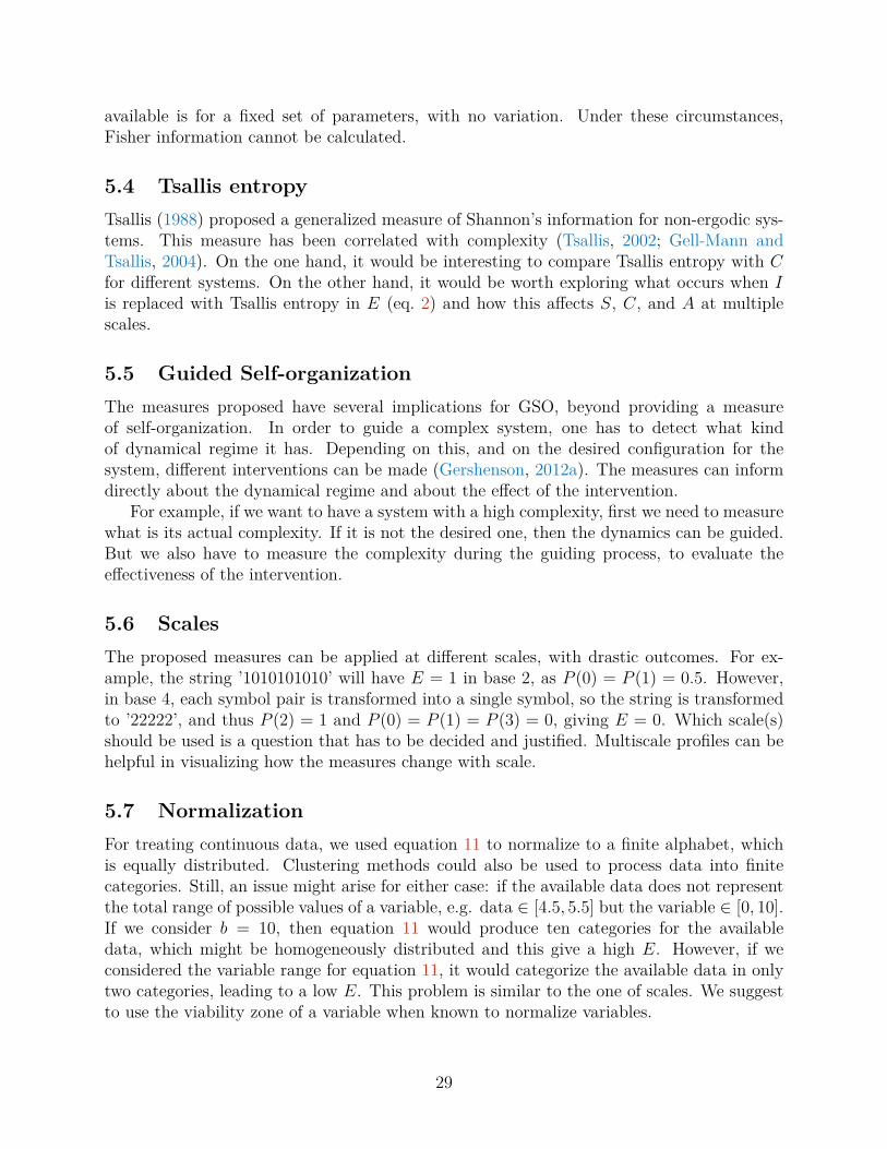
Figure 2 plots the measures proposed so far for different values of P (x). It can be seenthat E is maximal when P (x) = 0.5 and minimal when P (x) = 0 or P (x) = 1. The oppositeholds for S: it is minimal when P (x) = 0.5 and maximal when P (x) = 0 or P (x) = 1. C isminimal when S or E are minimal, i.e. P (x) = 0, P (x) = 0.5, or P (x) = 1. C is maximalwhen E = S = 0.5, which occurs when P (x) ≈ 0.11 or P (x) ≈ 0.89.

Shannon information can be seen as a balance of zeros and ones (maximal when P (0) =P (1) = 0.5), while C can be seen as a balance of E and S (maximal when E = S = 0.5).

3.4 HomeostasisThe previous three measures (E, S, and C) study how single variables change in time.To calculate the measures for a system, one can plot the histogram or simply average themeasures for all variables in a system. For homeostasis H, we are interested on how all

12

Table 1: Difference between observing single variables in time (columns) and several variablesat one time (rows).

X Y Zt = m− 2 xm−2 ym−2 zm−2t = m− 1 xm−1 ym−1 zm−1t = m xm ym zm

variables of a system change or not in time. Table 1 shows this difference: E, S, and Cfocusses on time series of variables (columns), while H focusses on states (rows).

Let X = x1x2x3...xn represent the state of a system of n variables (i.e. a row in Table 1).If the system has a high homeostasis, we would expect that its states do not change too muchin time. The homeostasis function H : Σ× Σ→ R should have the following properties:

1. The range is the real interval [0, 1].

2. H = 1 if and only if for states X and X ′, X = X ′, i.e. there is no change in time.

3. H = 0 if and only if ∀i, xi 6= x′i, i.e. all variables in the system changed.

A useful function for comparing strings of equal length is the Hamming distance. TheHamming distance d measures the percentage of different symbols in two strings X andX ′. For binary strings, it can be calculated with the XOR function (⊕). Its normalizationbounds the Hamming distance to the interval [0, 1]:

d(X,X ′) =

∑i∈{0,...,|X|}

xi ⊕ x′i

|X|. (7)

d measures the fraction of different symbols between X and X ′. For the Boolean case,d = 0 ⇐⇒ X = X ′ and d = 1 ⇐⇒ X = ¬X ′, while X and X ′ are uncorrelated⇐⇒ d ≈ 0.5.

We can use the inverse of d to define h:

h(X t, X t+1) = 1− d(X t, X t+1), (8)

which clearly fulfills the desired properties of homeostasis between two states.To measure the homeostasis of a system in time, we can generalize:

H = 1m− 1

m−1∑t=0

h(X t, X t+1), (9)

where m is the total number of time steps being evaluated. H will be simply the averageof different h from t = 0 to t = m− 1. As well as the previous measures based on I, H is aunitless measure.

13

When H is measured at higher scales, it can capture periodic dynamics. For example, letus have a system with n = 2 variables and a cycle of period 2: 11→ 00→ 11. H for base 2will be minimal, since every time step all variables change, i.e. ones turn into zeros or zerosturn into ones. However, if we measure H in base 4, then we will be actually comparingpairs of states, since to make one time step in base 4 we take two binary time steps. Thus,in base 4 the attractor becomes 22→ 22, and H = 1. The same applies for higher bases. Anexample of the usefulness of measuring H at multiple scales in elementary cellular automatais explained in Gershenson and Fernandez (2012).

3.5 AutopoiesisLet X represent the trajectories of the variables of a system and Y represent the trajectoriesof the variables of the environment of the system. A measure of autopoiesis A : Σ×Σ→ Rshould have the following properties:

1. A ≥ 0.

2. A should reflect the independence of X over Y . This implies:

(a) A > A′ ⇐⇒ X produces more of its own information than X ′ for a given Y .(b) A > A′ ⇐⇒ X produces more of its own information in Y than in Y ′.(c) A = A′ ⇐⇒ X produces as much of its own information than X ′ for a given Y .(d) A = A′ ⇐⇒ X produces as much of its own information in Y than in Y ′.(e) A = 0 if all of the information in X is produced by Y .

Following the classification of types of information transformation proposed in Gershen-son (2012b), dynamic and static transformations are internal (a system producing its owninformation), while active and stigmergic transformations are external (information producedby another system).

It is problematic to define in a general and direct way how some information dependson other information, as causality can be confounded with co-occurrence. For this reason,measures such as mutual information are not suitable for measuring A.

As it has been proposed, adaptive systems require a high C in order to be able to copewith changes of its environment while at the same time maintaining their integrity (Langton,1990; Kauffman, 1993). If X had a high E, then it would not be able to produce the samepatterns for different Y . With a high S, X would not be able to adapt to changes in Y .Therefore, we propose:

A = C(X)C(Y )

. (10)

If C(X) = 0, then either X is static (E(X) = 0) or pseudorandom (S(X) = 0). Thisimplies that any pattern (complexity) which could be observed in X (if any) should comefrom Y . This case gives a minimal A. On the other hand, if C(Y ) = 0, it implies thatany pattern (if any) in X should come from itself. This case gives a maximal A = ∞. A

14

particular case occurs if C(X) = 0 and C(Y ) = 0. A becomes undefined. But how can wesay something about autopoiesis if we are comparing two systems which are either withoutvariations (S = 1) or pseudorandom (E = 1)? This case should be undefined. The rest ofthe properties are evidently fulfilled by equation 10. This is certainly not the unique functionto fulfill the desired axioms. The exploration of alternatives requires further study.

Since A represents a ratio of probabilities, it is a unitless measure. A ∈ [0,∞), althoughit could be mapped to [0, 1) using a function such as f(A) = A

1+A. We do not normalize A

because it is useful to distinguish A > 1 and A < 1 (see Section 5.8).

3.6 Multi-scale profilesBar-Yam (2004) proposed the “complexity profile”, which plots the complexity of systemsdepending on the scale at which they are observed. This allows to compare how a measurechanges with scale. For example, the σ profile compares the “satisfaction” of systems atdifferent scales to study organization, evolution and cooperation (Gershenson, 2011).

In a similar way, multi-scale profiles can be used for each of the measures proposed, givingfurther insights about the dynamics of a system than measuring them at a single scale. Thisis clearly seen, for example, with different types of elementary cellular automata (Gershensonand Fernandez, 2012).

4 ResultsIn this section we apply the measures proposed in the previous section to two case studies:random Boolean networks and an aquatic ecosystem. A further case, elementary cellularautomata, can be found in Gershenson and Fernandez (2012).

4.1 Random Boolean NetworksResults show averages of 1000 RBNs, where 1000 steps were run from a random initial stateand E, S, C and H were calculated from data generated in 1000 additional steps.

R (R Project Contributors, 2012) was used with packages BoolNet (Mussel et al., 2010)and entropy (Hausser and Strimmer, 2012).

Figure 3 shows results for RBNs with 100 nodes, as the connectivity K varies. For lowK, there is high S and H, and a low E and C. This reflects the ordered regime of RBNs,where there is high robustness and few changes. Thus, it can be said that there is few or noinformation emerging and there is a high degree of self-organization and homeostasis. Forhigh K, there is high E, low S and C, and uncorrelated H ≈ 0.5. This reflects the chaoticregime of RBNs, where there is high fragility and many changes. Almost every bit (a newstate for most nodes) carries novel emergent information, and this constant change implieslow organization and complexity. For medium connectivities (2 ≤ K ≤ 3), there is a balancebetween E and S, leading to a high C. This corresponds to the critical regime of RBNs,which has been associated with complexity and the possibility of life (Kauffman, 2000).

As for autopoiesis, to model a system and its environment, we coupled two RBNs: One“internal” RBN with Ni nodes and Ki average connections and one “external” with Ne nodes

15

● ● ● ● ● ● ● ● ● ● ●● ●

●

● ●

●

●

●●

●●

●

●●

●

●●

●● ●

●● ● ● ● ● ● ● ● ● ● ● ● ● ● ● ● ● ●

0 1 2 3 4 5

0.0

0.2

0.4

0.6

0.8

1.0

K

I

● emergenceself−organizationhomeostasiscomplexity

Figure 3: Averages for 1000 RBNs, N = 100 nodes and varying average connectivity K(Gershenson and Fernandez, 2012).

and Ke average connections. A “coupled” RBN is considered with Nc = Ni +Ne nodes andKi connections. At every time step, the external RBN evolves independently. However,its state is copied to the Ne nodes representing it in the coupled RBN, which now evolvesdepending partly on the external RBN. Thus, the Ni nodes in the coupled RBN representingthe internal RBN may be affected by the dynamics of the external RBN, but not vice versa.The C of each node is calculated and averaged separately for each network, obtaining aninternal complexity Ci and an external complexity Ce.

Figure 4 and Table 2 show results for Ne = 96 and Ni = 32 for different combinations ofKe and Ki.

Table 2: A averages for 50 sets Ne = 96, Ni = 32. Same results as those shown in Figure 4.

Ki \Ke 1 2 3 4 51 0.4464025 0.5151070 0.7526248 1.6460345 3.40819672 1.6043330 0.9586809 1.1379227 2.0669794 3.24737293 2.4965328 0.9999926 0.9355231 1.3604272 2.62837984 2.1476247 0.7249803 0.6151742 0.8055051 1.38906305 1.8969094 0.4760027 0.3871875 0.4755580 0.8648389

As it was shown in Figure 3, C changes with K, so it is expected to have A ≈ 1 whenKi ≈ Ke. When Ce is high (Ke = 2 or Ke = 3), then the environment dominates thepatterns of the system, yielding A < 1. When Ce is low (Ke < 2 or Ke > 3), the patternsproduced by the system are not affected that much by its environment, thus A > 1, as long

16

1

2

3

4

5

1 2 3 4 5

Ki

Ke

Ni=

32

Ne = 96

●

●

●

●

●

●

●

Figure 4: A averages for 50 sets Ne = 96, Ni = 32. Values A < 1 are red while A > 1 areblue. Size of circles indicate how far A is from A = 1. Numerical values shown in Table 2.

17

as Ki < Ke (otherwise the system is more chaotic that its environment, and so complexpatterns have to come from outside).

A does not try to measure how much information emerges internally or externally, buthow much the patterns are internally or externally produced. A high E means that thereis no pattern, as there is constant change. A high S implies a static pattern. A high Creflects complex patterns. We are interested in A measuring the ratio of the complexity ofpatterns being produced by a system compared to the complexity of patterns produced byits environment.

4.2 An Ecological System: An Arctic LakeThe data from an Artic lake model used in this section was obtained using The AquaticEcosystem Simulator (Randerson and Bowker, 2008).

In general, Arctic lake systems are classified as oligotrophic due to their low primaryproduction, represented in chlorophyll values of 0.8-2.1 mg/m3. The lake’s water column, orlimnetic zone, is well-mixed; this means that there are no stratifications (layers with differenttemperatures). During winter (October to March), the surface of the lake is ice covered.During summer (April to September), ice melts and the water flow and evaporation increase,as shown in Figure 5A. Consequently, the two climatic periods (winter and summer) in theArctic region cause a typical hydrologic behavior in lakes as the one shown in Figure 5B.This hydrologic behavior influences the physiochemical subsystem of the lake.

Table 3 and Figure 6 show the variables and daily data we obtained from the Arctic lakesimulation. The model used is deterministic, so there is no variation in different simulationruns. Figure 6 depicts a high dispersion for the following variables: temperature (T ) andlight (L) at the three zones of the Arctic lake (surface=S, planktonic=P and benthic=B),inflow and outflow (IO), retention time (RT ) and evaporation (Ev). Ev is the variable withthe highest dispersion.

Observing RT and IO in logarithmic scale, we can see that their values are located atthe extremes, but their range is not long. Consequently, these variables have considerablevariability in a short range. However, the ranges of the other variables do not reflect largechanges. This situation complicates the interpretation and comparison of the physiochemicaldynamics. To attend this situation, we normalize the data to base b of all points x of allvariables X with the following equation:

f(x) =⌊b · x−minX

maxX −minX

⌋, (11)

where bxc is the floor function of x.Once all variables are in transformed into a finite alphabet, in this case, base 10 (b =

10), we can calculate emergence, self-organization, complexity, homeostasis and autopoiesis.Figure 7 depicts the number of points in each of the ten classes and shows the distributionof the values for each variable. Based on this distribution, the behavior for variables can beeasily described and compared. Variables with a more homogeneous distribution will producemore information, yielding higher values of emergence. Variables with a more heterogeneousdistribution will produce higher self-organization values. The complexity of variables is noteasy to deduce from Figure 7.

18

0 100 200 300

02

46

8

Days

Tem

pera

ture

(D

eg C

) SurfacePlanktonicBenthic

A

0 100 200 300

050

100

150

Days

Hyd

rolo

gy

Retention TimeInflow an outflowMixing ZoneWater Evaporation

B

Figure 5: (A) Climatic and (B) hydraulic regimes of Arctic lakes.

19

Table 3: Physiochemical variables considered in the Arctic lake model.Variable Units Acronym Max Min Median Mean std. dev.

Surface Light MJ/m2/day SL 30 1 5.1 11.06 11.27Planktonic Ligth MJ/m2/day PL 28.2 1 4.9 10.46 10.57Benthic Light MJ/m2/day BL 24.9 0.9 4.7 9.34 9.33Surface Temperature Deg C ST 8.6 0 1.5 3.04 3.34Planktonic Temperature Deg C PT 8.1 0.5 1.4 3.1 2.94Benthic Temperature Deg C BT 7.6 1.6 2 3.5 2.29Inflow and Outflow m3/sec IO 13.9 5.8 5.8 8.44 3.34Retention Time days RT 100 41.7 99.8 78.75 25.7Evaporation m3/day Ev 14325 0 2436.4 5065.94 5573.99Zone Mixing %/day ZM 55 45 50 50 3.54Inflow Conductivity uS/cm ICd 427 370.8 391.4 396.96 17.29Planktonic Conductivity uS/cm PCd 650.1 547.6 567.1 585.25 38.55Benthic Conductivity uS/cm BCd 668.4 560.7 580.4 600.32 40.84Surface Oxygen mg/litre SO2 14.5 11.7 13.9 13.46 1.12Planktonic Oxygen mg/litre PO2 13.1 10.5 12.6 12.15 1.02Benthic Oxygen mg/litre BO2 13 9.4 12.5 11.62 1.51Sediment Oxygen mg/litre SdO2 12.9 8.3 12.4 11.1 2.02Inflow pH ph Units IpH 6.4 6 6.2 6.2 0.15Planktonic pH ph Units PpH 6.7 6..40 6.6 6.57 0.09Benthic pH ph Units BpH 6.6 6.4 6.5 6.52 0.07

10

1000

SL PL BL ST PT BT I.O RT Ev ZM Icd PCd BCd SO2 PO2 BO2 SdO2 IpH PpH BpHvariable

valu

e

Figure 6: Boxplots of variables from the physiochemical subsystem. Abbreviations expandedin Table 3.

20

0

1

2

3

4

5

6

7

8

9

SL PL BL ST PT BT IO RT Ev ZM ICd PCd BCd SO2 PO2 BO2 SdO2 IpH PpH BpHvariable

valu

e

Figure 7: Transformed variables from the physiochemical subsystem to base 10.

4.2.1 Emergence, Self-organization, and Complexity

Figure 8 shows the values of emergence, self-organization, and complexity of the physio-chemical subsystem. Variables with a high complexity C ∈ [0.8, 1] reflect a balance betweenchange/chaos (emergence) and regularity/order (self-organization). This is the case of ben-thic and planktonic pH (BpH; PpH), IO (Inflow and Outflow) and RT (Retention Time).For variables with high emergencies (E > 0.92), like Inflow Conductivity (ICd) and ZoneMixing (ZM), their change in time is constant; a necessary condition for exhibiting chaos.For the rest of the variables, self-organization values are low (S < 0.32), reflecting low reg-ularity. It is interesting to notice that in this system there are no variables with a highself-organization nor low emergence.

Since E, S, C ∈ [0, 1], these measures can be categorized into five categories as shownin Table 4. These categories are described on the basis of the range value, the color andthe adjective in a scale from very high to very low. This categorization is inspired on thecategories for Colombian water pollution indices. These indices were proposed by Ramırezet al. (2003) and evaluated in Fernandez et al. (2005).

Table 4: Categories for classifying E, S, and C.Category Very High High Fair Low Very Low

Range [0.8, 1] [0.6, 0.8) [0.4, 0.6) [0.2, 0.4) [0, 0.2)Color Blue Green Yellow Orange Red

Table 5 shows results of E, S, and C using the categories just mentioned.From Table 5 and a principal component analysis (not shown), we can divide the values

obtained in complexity categories as follows:

21

SL PL BL ST PT BT IO RT Ev ZM ICd PCd BCd SO2 PO2 BO2 SdO2 IpH PpH BpH

Emergence0.

00.

20.

40.

60.

81.

0

SL PL BL ST PT BT IO RT Ev ZM ICd PCd BCd SO2 PO2 BO2 SdO2 IpH PpH BpH

Self−organization

0.0

0.2

0.4

0.6

0.8

1.0

SL PL BL ST PT BT IO RT Ev ZM ICd PCd BCd SO2 PO2 BO2 SdO2 IpH PpH BpH

Complexity

0.0

0.2

0.4

0.6

0.8

1.0

0 100 200 300

0.0

0.2

0.4

0.6

0.8

1.0

Homeostasis

Figure 8: E, S, and C of physiochemical variables of the Arctic lake model (also shown inTable 5) and daily variations of homeostasis H during a simulated year.

Table 5: E, S, and C of physiochemical variables of the Arctic lake model. Also shown inFigure 2.

Variable Acronym E S C

Benthic pH BpH 0.44196793 0.55803207 0.98652912In and Outflow IO 0.52310253 0.47689747 0.99786509Retention Time RT 0.53890552 0.46109448 0.99394544Planktonic pH PpH 0.54122993 0.45877007 0.99320037Sediment Oxygen SdO2 0.59328705 0.40671295 0.96519011Benthic Oxygen BO2 0.67904928 0.32095072 0.87176542Inflow pH IpH 0.69570975 0.30429025 0.84679077Benthic Temperature BT 0.72661539 0.27338461 0.79458186Planktonic Temperature PT 0.75293885 0.24706115 0.74408774Planktonic Light PL 0.75582978 0.24417022 0.7382045Surface Light SL 0.75591484 0.24408516 0.73803038Benthic Light BL 0.76306133 0.23693867 0.72319494Surface Oxygen SO2 0.76509182 0.23490818 0.71890531Surface Temperature ST 0.76642121 0.23357879 0.71607895Evaporation Ev 0.76676234 0.23323766 0.71535142Planktonic Oxygen PO2 0.76887287 0.23112713 0.71082953Benthic Conductivity BCd 0.77974428 0.22025572 0.68697255Planktonic Conductivity PCd 0.78604873 0.21395127 0.6727045Inflow Conductivity ICd 0.92845597 0.07154403 0.26570192Zone Mixing ZM 0.94809050 0.0519095 0.1968596

22

Very High Complexity : C ∈ [0.8, 1]. The following variables balance self-organizationand emergence: benthic and planktonic pH (BpH, PpH), inflow and outflow (IO), andretention time (RT ). It is remarkable that the increasing of the hydrological regimeduring summer is related in an inverse way with the dissolved oxygen (SO2; BO2).It means that an increased flow causes oxygen depletion. Benthic Oxygen (BO2) andInflow Ph (IpH) show the lowest levels of the category. Between both, there is anegative correlation: a doubling of IpH is associated with a decline of BO2 in 40%.

High Complexity : C ∈ [0.6, 0.8). This group includes 11 of the 21 variables and involvesa high E and a low S. These 11 variables that showed more chaotic than orderedstates are highly influenced by the solar radiation that defines the winter and summerseasons, as well as the hydrological cycle. These variables were: Oxygen (PO2, SO2);surface, planktonic and benthic temperature (ST , PT , BT ); conductivity (ICd, PCd,BCd); planktonic and benthic light (PL,BL); and evaporation (Ev).

Very Low Complexity : C ∈ [0, 0.2). In this group, E is very high, and S is verylow. This category includes the inflow conductivity (ICd) and water mixing variance(ZM). Both are high and directly correlated; it means that an increase of the mixingpercentage between planktonic and benthic zones is associated with an increase ofinflow conductivity.

4.2.2 Homeostasis

The homeostasis was calculated by comparing the daily values of all variables, representingthe state of the Arctic subsystem. The temporal timescale is very important, because H canvary considerably if we compare states every minute or every month.

The h values have a mean (H) of 0.95739726 and a standard deviation of 0.064850247.The minimum h is 0.60 and the maximum h is 1.0. In an annual cycle, homeostasis showsfour different patterns, as shown in Figure 8, which correspond with the seasonal variationsbetween winter and summer. These four periods show scattered values of homeostasis asthe result of transitions between winter and summer and winter back again. The winterperiod (first and last days of the year) has very high h levels (1 or close to 1) and startsfrom day 212 and goes to day 87. In this period, the winter conditions such as low lightlevel, temperature, maximum time retention due to ice covering, low inflow and outflow,water mixing interchange between planktonic and benthic zones, low conductivities and pHsand high oxygen are present. The second, third and fourth periods correspond to summer.The second period starts with an increase of benthic pH, zone mixing, and inflow-outflowvariables. Between days 83 and 154, this period is characterized for extreme fluctuationsas a result of an increase in temperature and light. Homeostasis fluctuates and reaches aminimum of 0.6 in day 116. At the end of this period, the evaporation and zone mixingincrease, while oxygen decreases in the benthic zone and sediment. The third period (days155 to 162) reflects the stabilization of the summer conditions; It means maximum evapo-ration, temperature, light, mixing zone, conductivity and pH and the lowest oxygen level.Homeostasis is maximal again for this period. The fourth period (days 163-211), which hash fluctuations near 0.9, corresponds to the transition of summer to winter conditions.

As it can be seen, using h, periodic or seasonal dynamics can be followed and studied.

23

4.2.3 Autopoiesis

Autopoiesis was measured for three components (subsystems) at the planktonic and benthiczones of the Arctic lake. These were physiochemical, limiting nutrients and biomass. Theyinclude the variables and organisms related in Table 6.

Table 6: Variables and organisms used for calculatingautopoiesis.

Component Planktonic zone Benthic zonePhysiochemical Light, Temperature, Conduc-

tivity, Oxygen, pH.Light, Temperature, Conduc-tivity, Oxygen, Sediment Oxy-gen, pH.

Limiting Nutri-ents

Silicates, Nitrates, Phosphates,Carbon Dioxide.

Silicates, Nitrates, Phosphates,Carbon Dioxide.

Biomass Diatoms, Cyanobacteria,Green Algae, Chlorophyta.

Diatoms, Cyanobacteria,Green Algae.

According to the complexity categories established in Table 4, the planktonic and ben-thic components have been classified in the following categories: limiting nutrient variablesin the low complexity category (C ∈ [0.2, 0.4); orange color), planktonic physiochemicalvariables in the high complexity category (C ∈ [0.6, 0.8); green color) and biomass andbenthic physiochemical variables in the very high complexity category (C ∈ [0.8, 1]; bluecolor). A comparison of the complexity level for each subsystem of each zone (averagingtheir respective variables) is depicted in Figure 9.

Planktonic (P) Benthic (B)

Limiting Nutrient, Physiochemical and Biomass

Lake Zone

Com

plex

ity

0.0

0.2

0.4

0.6

0.8

1.0

Figure 9: C of planktonic and benthic components.

In order to compare the autonomy of each group of variables, equation 10 was appliedto the complexity data, as shown in Figure 10. For the planktonic and benthic zones, wecalculated the autopoiesis of the biomass elements in relation to limiting nutrient and phys-iochemical variables. All A values are greater than 1. This means that the variables related

24

to living systems have a greater complexity than the variables related to their environment,represented by the limiting nutrient and physiochemical variables. While we can say thatsome physiochemical variables, including limiting nutrients have more or fewer effects on theplanktonic and benthic biomass, we can also estimate that planktonic and benthic biomassare more autonomous compared to their physiochemical and nutrient environments. The veryhigh values of complexity of biomass imply that these living systems can adapt to the changesof their environments because of the balance between emergence and self-organization thatthey have.

Planktonic Zone Benthic Zone

PB/LN and PB/PC

Lake Zone

Aut

opoi

esis

0.0

0.5

1.0

1.5

2.0

2.5

3.0

Figure 10: A of biomass depending on limiting nutrients and physiochemical components.

4.2.4 Multiple scales

The previous analysis of the Arctic lake was performed using base ten. We obtained themeasures for the same data using bases 2i,∀i ∈ [1..6], as shown in Figures 11 and 12.

For base 2 (Figure 11A), there is a very high E for all variables, as the richness of thedynamics cannot be captured by only two values. Thus, S and C are low. Base 8 (Figure 11C)gives results very similar to those of base 10 (Figure 8), indicating that the measures are notsensitive to slight changes of base. Base 4 (Figure 11B) gives intermediate values betweenbase 2 and base 8. Results for bases 16, 32, and 64 (Figure 12) are very similar to those ofbase 10 and 8, showing that the choice of base is relevant but not a sensitive parameter.

As more diversity is possible with higher bases, homeostasis values decrease with base.Still, the different periods of the year can be identified at all scales, with different levels ofdetail.

In the case of the Arctic lake model, studying the dynamics with a single base, i.e. at asingle scale, can be very informative. However, studying the same phenomena at multiplescales can give further insights, independently on whether the measures change or not withscale.

25

SL PL BL ST PT BT IO RT Ev ZM ICd PCd BCd SO2 PO2 BO2 SdO2 IpH PpH BpH

Emergence0.

00.

20.

40.

60.

81.

0

SL PL BL ST PT BT IO RT Ev ZM ICd PCd BCd SO2 PO2 BO2 SdO2 IpH PpH BpH

Self−organization

0.0

0.2

0.4

0.6

0.8

1.0

SL PL BL ST PT BT IO RT Ev ZM ICd PCd BCd SO2 PO2 BO2 SdO2 IpH PpH BpH

Complexity

0.0

0.2

0.4

0.6

0.8

1.0

0 100 200 300

0.0

0.2

0.4

0.6

0.8

1.0

Homeostasis

A. Base 2.

SL PL BL ST PT BT IO RT Ev ZM ICd PCd BCd SO2 PO2 BO2 SdO2 IpH PpH BpH

Emergence

0.0

0.2

0.4

0.6

0.8

1.0

SL PL BL ST PT BT IO RT Ev ZM ICd PCd BCd SO2 PO2 BO2 SdO2 IpH PpH BpH

Self−organization

0.0

0.2

0.4

0.6

0.8

1.0

SL PL BL ST PT BT IO RT Ev ZM ICd PCd BCd SO2 PO2 BO2 SdO2 IpH PpH BpH

Complexity

0.0

0.2

0.4

0.6

0.8

1.0

0 100 200 300

0.0

0.2

0.4

0.6

0.8

1.0

Homeostasis

B. Base 4.

SL PL BL ST PT BT IO RT Ev ZM ICd PCd BCd SO2 PO2 BO2 SdO2 IpH PpH BpH

Emergence

0.0

0.2

0.4

0.6

0.8

1.0

SL PL BL ST PT BT IO RT Ev ZM ICd PCd BCd SO2 PO2 BO2 SdO2 IpH PpH BpH

Self−organization

0.0

0.2

0.4

0.6

0.8

1.0

SL PL BL ST PT BT IO RT Ev ZM ICd PCd BCd SO2 PO2 BO2 SdO2 IpH PpH BpH

Complexity

0.0

0.2

0.4

0.6

0.8

1.0

0 100 200 300

0.0

0.2

0.4

0.6

0.8

1.0

Homeostasis

C. Base 8.

Figure 11: Emergence, Self-organization, Complexity, and Homeostasis for Arctic lake modelat multiple scales: 2, 4, and 8.

26

SL PL BL ST PT BT IO RT Ev ZM ICd PCd BCd SO2 PO2 BO2 SdO2 IpH PpH BpH

Emergence0.

00.

20.

40.

60.

81.

0

SL PL BL ST PT BT IO RT Ev ZM ICd PCd BCd SO2 PO2 BO2 SdO2 IpH PpH BpH

Self−organization

0.0

0.2

0.4

0.6

0.8

1.0

SL PL BL ST PT BT IO RT Ev ZM ICd PCd BCd SO2 PO2 BO2 SdO2 IpH PpH BpH

Complexity

0.0

0.2

0.4

0.6

0.8

1.0

0 100 200 300

0.0

0.2

0.4

0.6

0.8

1.0

Homeostasis

A. Base 16.

SL PL BL ST PT BT IO RT Ev ZM ICd PCd BCd SO2 PO2 BO2 SdO2 IpH PpH BpH

Emergence

0.0

0.2

0.4

0.6

0.8

1.0

SL PL BL ST PT BT IO RT Ev ZM ICd PCd BCd SO2 PO2 BO2 SdO2 IpH PpH BpH

Self−organization

0.0

0.2

0.4

0.6

0.8

1.0

SL PL BL ST PT BT IO RT Ev ZM ICd PCd BCd SO2 PO2 BO2 SdO2 IpH PpH BpH

Complexity

0.0

0.2

0.4

0.6

0.8

1.0

0 100 200 300

0.0

0.2

0.4

0.6

0.8

1.0

Homeostasis

B. Base 32.

SL PL BL ST PT BT IO RT Ev ZM ICd PCd BCd SO2 PO2 BO2 SdO2 IpH PpH BpH

Emergence

0.0

0.2

0.4

0.6

0.8

1.0

SL PL BL ST PT BT IO RT Ev ZM ICd PCd BCd SO2 PO2 BO2 SdO2 IpH PpH BpH

Self−organization

0.0

0.2

0.4

0.6

0.8

1.0

SL PL BL ST PT BT IO RT Ev ZM ICd PCd BCd SO2 PO2 BO2 SdO2 IpH PpH BpH

Complexity

0.0

0.2

0.4

0.6

0.8

1.0

0 100 200 300

0.0

0.2

0.4

0.6

0.8

1.0

Homeostasis

C. Base 64.

Figure 12: Emergence, Self-organization, Complexity, and Homeostasis for Arctic lake modelat multiple scales: 16, 32, and 64.

27

5 Discussion

5.1 MeasuresThe proposed measures characterize the different configurations and dynamics that elementsof complex systems acquire through their interactions. Just like temperature averages thekinetic energy of molecules, much information is lost in the averaging, as the description ofphenomena changes scale. The measures are probabilistic (except for H) and they all relyon statistical samples7. Thus, the caveats of statistics and probability should be taken intoconsideration when using the proposed measures. Still, these measures capture the propertiesand tendencies of a system, that is why the scale at which they are described is important.They will not indicate which element interacted with which element, how and when. If weare interested in the properties and tendencies of the elements, we can change scale andapply the measures there. Still, we have to be aware that the measures are averaging—andthus simplifying—the phenomena they describe. Whether relevant information is lost on theaveraging depends not only on the phenomenon, but on what kind of information we areinterested in, i.e. relevance is also partially dependent on the observer (Gershenson, 2002).

5.2 Complexity as balance or entropy?Some approaches relate complexity with a high entropy, i.e. information content (Bar-Yam,2004; Delahaye and Zenil, 2007). Just as chaos should not be confused with complexity (Ger-shenson, 2013), a very high entropy (high emergence E) implies too much change, wherecomplex patterns are destroyed. On the other hand, very low entropy (high self-organizationS), prevents complex patterns from emerging. As it has been proposed by several authors,complexity can be seen as balance between order and disorder (Langton, 1990; Kauffman,1993; Lopez-Ruiz et al., 1995), and thus, it is logical to postulate C as a balance of E andS.

It might seem contradictory to define emergence as the opposite of self-organization, asthey are both present in several complex phenomena. However, when one takes one to theextreme (emergence or self-organization), the other is negligible. It is precisely when both ofthem are balanced that complexity occurs, but this does not mean that both of them haveto be maximal.

5.3 Fisher InformationC is correlated with Fisher information, which has been shown to be related to phase tran-sitions (Prokopenko et al., 2011). Following the view of high complexity as a balance, itis natural that C is maximal at phase transitions, which is the case for both C and Fisherinformation. However, the steepness of Fisher information is much higher than that of C. Itis appropriate for determining phase transitions, but it makes little distinction of dynamicsfarther from transitions. C is smoother, so it can represent dynamical change in a moregradual fashion. Moreover, to calculate Fisher information, a parameter must be varied,which limits its applicability for analyzing real data. This is because in many cases the data

7This is also the reason for why all measures are unitless.

28

available is for a fixed set of parameters, with no variation. Under these circumstances,Fisher information cannot be calculated.

5.4 Tsallis entropyTsallis (1988) proposed a generalized measure of Shannon’s information for non-ergodic sys-tems. This measure has been correlated with complexity (Tsallis, 2002; Gell-Mann andTsallis, 2004). On the one hand, it would be interesting to compare Tsallis entropy with Cfor different systems. On the other hand, it would be worth exploring what occurs when Iis replaced with Tsallis entropy in E (eq. 2) and how this affects S, C, and A at multiplescales.

5.5 Guided Self-organizationThe measures proposed have several implications for GSO, beyond providing a measureof self-organization. In order to guide a complex system, one has to detect what kindof dynamical regime it has. Depending on this, and on the desired configuration for thesystem, different interventions can be made (Gershenson, 2012a). The measures can informdirectly about the dynamical regime and about the effect of the intervention.

For example, if we want to have a system with a high complexity, first we need to measurewhat is its actual complexity. If it is not the desired one, then the dynamics can be guided.But we also have to measure the complexity during the guiding process, to evaluate theeffectiveness of the intervention.

5.6 ScalesThe proposed measures can be applied at different scales, with drastic outcomes. For ex-ample, the string ’1010101010’ will have E = 1 in base 2, as P (0) = P (1) = 0.5. However,in base 4, each symbol pair is transformed into a single symbol, so the string is transformedto ’22222’, and thus P (2) = 1 and P (0) = P (1) = P (3) = 0, giving E = 0. Which scale(s)should be used is a question that has to be decided and justified. Multiscale profiles can behelpful in visualizing how the measures change with scale.

5.7 NormalizationFor treating continuous data, we used equation 11 to normalize to a finite alphabet, whichis equally distributed. Clustering methods could also be used to process data into finitecategories. Still, an issue might arise for either case: if the available data does not representthe total range of possible values of a variable, e.g. data ∈ [4.5, 5.5] but the variable ∈ [0, 10].If we consider b = 10, then equation 11 would produce ten categories for the availabledata, which might be homogeneously distributed and this give a high E. However, if weconsidered the variable range for equation 11, it would categorize the available data in onlytwo categories, leading to a low E. This problem is similar to the one of scales. We suggestto use the viability zone of a variable when known to normalize variables.

29

5.8 Autopoiesis and Requisite VarietyAshby’s Law of Requisite Variety (Ashby, 1956) states that an active controller requires asmuch variety (number of states) as that of the controlled system to be stable. For example,if a system can be in four different states, its controller must be able to discriminate betweenthose four states in order to regulate the dynamics of the system.

The proposed measure of autopoiesis is related to the law of requisite variety, as a systemwith a A > 1 must have a higher complexity (variety) than its environment, also reflectingits autonomy. Thus, a successful controller should have A > 1 (at multiple scales (Gershen-son, 2011)), although the controller will be more efficient if A → 1, assuming that highercomplexities have higher costs.

6 ConclusionsWe reviewed measures of emergence, self-organization, complexity, homeostasis, and au-topoiesis based on information theory. Axioms were postulated for each measure and equa-tions were derived form them. Having in mind that there are several different measuresalready proposed (Prokopenko et al., 2009; Gershenson and Fernandez, 2012), this approachallows us to evaluate the axioms underlying the measures, as opposed to trying to comparedifferent measures without a common ground.

The generality and usefulness of the proposed measures will be evaluated gradually, asthese are applied to different systems. These can be abstract (e.g. Turing machines (Delahayeand Zenil, 2007, 2012), ε-machines (Shalizi and Crutchfield, 2001; Gornerup and Crutchfield,2008)), biological (ecosystems, organisms), economic, social or technological (Helbing, 2011).

The potential benefits of general measures as the ones proposed here are manifold. Evenif with time more appropriate measures are found, aiming at the goal of finding generalmeasures which can characterize complexity, emergence, self-organization, homeostasis, au-topoiesis, and related concepts for any observable system is a necessary step to take.

AcknowledgementsWe should like to thank Nihat Ay, Ragnar Behncke, Paul Bourgine, Niccolo Capanni, WilfriedElmenreich, Tom Froese, Virgil Griffith, Joseph Lizier, Luis Miramontes-Hercog, RobertoMurcio, Oliver Obst, Daniel Polani, Mikhail Prokopenko, Robert Ulanowicz, Rosalind Wang,and an anonymous referee for interesting critiques, discussions, and suggestions. DiegoLizcano and Cristian Villate helped with programming tasks. Figure 1 was made by AlbanBlanco. C. G. was partially supported by SNI membership 47907 of CONACyT, Mexico.

ReferencesAldana-Gonzalez, M., Coppersmith, S., and Kadanoff, L. P. (2003). Boolean

dynamics with random couplings. In Perspectives and Problems in Nonlinear Science.A Celebratory Volume in Honor of Lawrence Sirovich, E. Kaplan, J. E. Marsden, and

30

K. R. Sreenivasan, (Eds.). Springer Appl. Math. Sci. Ser.. URL http://www.fis.unam.mx/%7Emax/PAPERS/nkreview.pdf.

Anderson, P. W. (1972). More is different. Science 177: 393–396.

Ash, R. B. (1990). Information Theory. Dover Publications, Inc.

Ashby, W. R. (1947a). The nervous system as physical machine: With special reference tothe origin of adaptive behavior. Mind 56 (221) (January): 44–59. URL http://tinyurl.com/aqcmdy.

Ashby, W. R. (1947b). Principles of the self-organizing dynamic system. Journal of GeneralPsychology 37: 125–128.

Ashby, W. R. (1956). An Introduction to Cybernetics. Chapman & Hall, London. URLhttp://pcp.vub.ac.be/ASHBBOOK.html.

Ashby, W. R. (1960). Design for a brain: The origin of adaptive behaviour , 2nd ed.Chapman & Hall, London. URL http://dx.doi.org/10.1037/11592-000.

Ay, N., Der, R., and Prokopenko, M. (2012). Guided self-organization: perception–action loops of embodied systems. Theory in Biosciences 131 (3): 125–127. URL http://dx.doi.org/10.1007/s12064-011-0140-1.

Bar-Yam, Y. (1997). Dynamics of Complex Systems. Studies in Nonlinearity. WestviewPress, Boulder, CO, USA. URL http://www.necsi.org/publications/dcs/.

Bar-Yam, Y. (2004). Multiscale variety in complex systems. Complexity 9 (4): 37–45.URL http://necsi.org/projects/yaneer/multiscalevariety.pdf.

Bernard, C. (1859). Lecons sur les proprietes physiologiques et les alterations pathologiquesdes liquides de l’organisme. Paris.

Camazine, S., Deneubourg, J.-L., Franks, N. R., Sneyd, J., Theraulaz, G., andBonabeau, E. (2003). Self-Organization in Biological Systems. Princeton UniversityPress, Princeton, NJ, USA. URL http://www.pupress.princeton.edu/titles/7104.html.

Cannon, W. (1932). The wisdom of the body. WW Norton & Co, New York.

Delahaye, J.-P. and Zenil, H. (2007). On the Kolmogorov-Chaitin complexity for shortsequences. In Randomness and Complexity: From Leibniz to Chaitin, C. S. Calude, (Ed.).World Scientific, Singapore, 123. URL http://arxiv.org/abs/0704.1043.

Delahaye, J.-P. and Zenil, H. (2012). Numerical evaluation of algorithmic complexityfor short strings: A glance into the innermost structure of randomness. Applied Math-ematics and Computation 219 (1) (September): 63–77. URL http://dx.doi.org/10.1016/j.amc.2011.10.006.

31

Di Paolo, Ezequiel, A. (2000). Homeostatic adaptation to inversion of the visual fieldand other sensorimotor disruptions. In From animals to animats 6: Proceedings of the 6thInternational Conference on the Simulation of Adaptive Behavior, J.-A. Meyer, A. Berthoz,D. Floreano, H. Roitblat, and S. W. Wilson, (Eds.). MIT Press, 440–449. URL http://sro.sussex.ac.uk/29695/.

Edmonds, B. (1999). Syntactic measures of complexity. Ph.D. thesis, University of Manch-ester, Manchester, UK. URL http://bruce.edmonds.name/thesis/.

Fernandez, N., Aguilar, J., Gershenson, C., and Teran, O. (2012). Sistemasdinamicos como redes computacionales de agentes para la evaluacion de sus propiedadesemergentes. In II Simposio Cientıfico y Tecnologico en Computacion SCTC 2012. Univer-sidad Central de Venezuela.

Fernandez, N., Ramırez, A., and Solano, F. (2005). Physico-chemical wa-ter quality indices. BISTUA 2: 19–30. URL http://www.academia.edu/193200/PHYSICO-CHEMICAL_WATER_QUALITY_INDICES.

Froese, T. and Stewart, J. (2010). Life After Ashby: Ultrastability and the AutopoieticFoundations of Biological Autonomy. Cybernetics and Human Knowing 17 (4): 7–50. URLhttp://tinyurl.com/cw6b57e.

Gell-Mann, M. and Tsallis, C., Eds. (2004). Nonextensive Entropy - InterdisciplinaryApplications. Oxford University Press.

Gershenson, C. (2002). Contextuality: A philosophical paradigm, with applications tophilosophy of cognitive science. POCS Essay, COGS, University of Sussex. URL http://cogprints.org/2621/.

Gershenson, C. (2004). Introduction to random Boolean networks. In Workshop andTutorial Proceedings, Ninth International Conference on the Simulation and Synthesis ofLiving Systems (ALife IX), M. Bedau, P. Husbands, T. Hutton, S. Kumar, and H. Suzuki,(Eds.). Boston, MA, pp. 160–173. URL http://arxiv.org/abs/nlin.AO/0408006.

Gershenson, C. (2007). Design and Control of Self-organizing Systems. CopIt Arxives,Mexico. http://tinyurl.com/DCSOS2007. URL http://tinyurl.com/DCSOS2007.

Gershenson, C. (2011). The sigma profile: A formal tool to study organization and itsevolution at multiple scales. Complexity 16 (5): 37–44. URL http://arxiv.org/abs/0809.0504.

Gershenson, C. (2012a). Guiding the self-organization of random Boolean networks.Theory in Biosciences 131 (3) (September): 181–191. URL http://arxiv.org/abs/1005.5733.

Gershenson, C. (2012b). The world as evolving information. In Unifying Themes inComplex Systems, A. Minai, D. Braha, and Y. Bar-Yam, (Eds.). Vol. VII. Springer, BerlinHeidelberg, 100–115. URL http://arxiv.org/abs/0704.0304.

32

Gershenson, C. (2013). The implications of interactions for science and philosophy. Foun-dations of Science Early View. URL http://arxiv.org/abs/1105.2827.

Gershenson, C., Aerts, D., and Edmonds, B., Eds. (2007). Philosophy and Com-plexity. Worldviews, Science and Us. World Scientific, Singapore. URL http://www.worldscibooks.com/chaos/6372.html.

Gershenson, C. and Fernandez, N. (2012). Complexity and information: Measuringemergence, self-organization, and homeostasis at multiple scales. Complexity 18 (2): 29–44. URL http://dx.doi.org/10.1002/cplx.21424.

Gershenson, C. and Heylighen, F. (2003). When can we call a system self-organizing?In Advances in Artificial Life, 7th European Conference, ECAL 2003 LNAI 2801,W. Banzhaf, T. Christaller, P. Dittrich, J. T. Kim, and J. Ziegler, (Eds.). Springer, Berlin,pp. 606–614. URL http://arxiv.org/abs/nlin.AO/0303020.

Gleick, J. (2011). The information: A history, a theory, a flood. Pantheon, New York.

Gornerup, O. and Crutchfield, J. P. (2008). Hierarchical self-organization in thefinitary process soup. Artificial Life 14 (3) (Summer): 245–254. Special Issue on theEvolution of Complexity. URL http://tinyurl.com/266j3w.

Hausser, J. and Strimmer, K. (2012). R package ‘entropy’. v. 1.1.7.

Helbing, D. (2011). FuturICT - new science and technology to manage our complex,strongly connected world. arXiv:1108.6131. URL http://arxiv.org/abs/1108.6131.

Heylighen, F., Cilliers, P., and Gershenson, C. (2007). Complexity and philosophy.In Complexity, Science and Society, J. Bogg and R. Geyer, (Eds.). Radcliffe Publishing,Oxford, 117–134. URL http://arxiv.org/abs/cs.CC/0604072.

Holzer, R. and De Meer, H. (2011). Methods for approximations of quantitative mea-sures in self-organizing systems. In Self-Organizing Systems, C. Bettstetter and C. Ger-shenson, (Eds.). Lecture Notes in Computer Science, vol. 6557. Springer, Berlin / Heidel-berg, 1–15. URL http://dx.doi.org/10.1007/978-3-642-19167-1_1.

Jen, E., Ed. (2005). Robust Design: A Repertoire of Biological, Ecological, and EngineeringCase Studies. Santa Fe Institute Studies on the Sciences of Complexity. Oxford UniversityPress, Oxford, UK. URL http://tinyurl.com/swtlz.

Kauffman, S. A. (1969). Metabolic stability and epigenesis in randomly constructedgenetic nets. Journal of Theoretical Biology 22: 437–467.

Kauffman, S. A. (1993). The Origins of Order. Oxford University Press, Oxford, UK.

Kauffman, S. A. (2000). Investigations. Oxford University Press, Oxford, UK.

Langton, C. (1990). Computation at the edge of chaos: Phase transitions and emergentcomputation. Physica D 42: 12–37.

33

Lloyd, S. (2001). Measures of complexity: a non-exhaustive list. Department of MechanicalEngineering, Massachusetts Institute of Technology. URL http://web.mit.edu/esd.83/www/notebook/Complexity.PDF.

Lopez-Ruiz, R., Mancini, H. L., and Calbet, X. (1995). A statistical measure ofcomplexity. Physics Letters A 209 (5-6): 321–326. URL http://dx.doi.org/10.1016/0375-9601(95)00867-5.

Luisi, P. L. (2003). Autopoiesis: a review and a reappraisal. Naturwissenschaften 90 (2):49–59. URL http://dx.doi.org/10.1007/s00114-002-0389-9.

Maturana, H. (2011). Ultrastability...Autopoiesis? Reflective Response to Tom Froese andJohn Stewart. Cybernetics Human Knowing 18 (1-2): 143–152. URL http://tinyurl.com/d9jrswn.

Maturana, H. and Varela, F. (1980). Autopoiesis and Cognition: The realization ofliving. Reidel Publishing Company, Dordrecht.

Mitchell, M. (2009). Complexity: A Guided Tour. Oxford University Press, Oxford, UK.

Morin, E. (2007). Restricted complexity, general complexity. In Philosophy and Complexity,C. Gershenson, D. Aerts, and B. Edmonds, (Eds.). Worldviews, Science and Us. WorldScientific, Singapore, 5–29. Translated from French by Carlos Gershenson. URL http://tinyurl.com/b9quxon.

Mussel, C., Hopfensitz, M., and Kestler, H. A. (2010). BoolNet – an R packagefor generation, reconstruction and analysis of Boolean networks. Bioinformatics 26 (10):1378–1380.

Polani, D., Prokopenko, M., and Yaeger, L. S. (2013). Information and self-organization of behavior. Advances in Complex Systems 16 (2&3): 1303001. URLhttp://dx.doi.org/10.1142/S021952591303001X.

Prokopenko, M. (2009). Guided self-organization. HFSP Journal 3 (5): 287–289. URLhttp://dx.doi.org/10.2976/1.3233933.

Prokopenko, M., Boschetti, F., and Ryan, A. J. (2009). An information-theoreticprimer on complexity, self-organisation and emergence. Complexity 15 (1): 11–28. URLhttp://dx.doi.org/10.1002/cplx.20249.

Prokopenko, M., Lizier, J. T., Obst, O., and Wang, X. R. (2011). Relating Fisherinformation to order parameters. Phys. Rev. E 84: 041116. URL http://dx.doi.org/10.1103/PhysRevE.84.041116.

R Project Contributors. (2012). The R project for statistical computing. URL http://www.r-project.org/.

Ramırez, A., Restrepo, R., and Fernandez, N. (2003). Evaluacion de impactosambientales causados por vertimientos sobre aguas continentales. Ambiente y Desarrollo 2:56–80. URL http://www.javeriana.edu.co/fear/ins_amb/rad12-13.htm.

34

Randerson, P. and Bowker, D. (2008). Aquatic Ecosystem Simulator (AES) — a learn-ing resource for biological science students. URL http://www.bioscience.heacademy.ac.uk/resources/projects/randerson.aspx.

Ruiz-Mirazo, K. and Moreno, A. (2004). Basic autonomy as a fundamnental step inthe synthesis of life. Artificial Life 10 (3) (Summer): 235–259.

Seidl, D. (2004). Luhmann’s theory of autopoietic social systems. Tech. Rep. 2004-2,Ludwig-Maximilians-Universitat Munchen. Munich Business Research paper.

Shalizi, C. and Crutchfield, J. (2001). Computational mechanics: Pattern and pre-diction, structure and simplicity. Journal of Statistical Physics 104: 816–879. URLhttp://arxiv.org/abs/cond-mat/9907176.

Shalizi, C. R. (2001). Causal architecture, complexity and self-organization in time seriesand cellular automata. Ph.D. thesis, University of Wisconsin at Madison. URL http://tinyurl.com/v3lho.

Shannon, C. E. (1948). A mathematical theory of communication. Bell System TechnicalJournal 27: 379–423 and 623–656. URL http://tinyurl.com/6qrcc.

Stumm, W. (2004). Chemical Processes Regulating the Composition of Lake Waters. In TheLakes Handbook Vol 1. Limonlogy and Limnetic Ecology, P. O’Sullivan and C. Reynolds,(Eds.). Blackwell Science Ltd, Malden, USA, Chapter 5, pp. 79–106.

Tsallis, C. (1988). Possible generalization of Boltzmann-Gibbs statistics. Journal ofStatistical Physics 52 (1-2): 479–487. URL http://dx.doi.org/10.1007/BF01016429.

Tsallis, C. (2002). Entropic nonextensivity: a possible measure of complexity. Chaos, Soli-tons & Fractals 13 (3): 371 – 391. URL http://dx.doi.org/10.1016/S0960-0779(01)00019-4.

Varela, F. G., Maturana, H. R., and Uribe, R. (1974). Autopoiesis: The organizationof living systems, its characterization and a model. Biosystems 5 (4): 187–196. URLhttp://dx.doi.org/10.1016/0303-2647(74)90031-8.

Wagner, A. (2005). Robustness and Evolvability in Living Systems. Princeton UniversityPress, Princeton, NJ. URL http://www.pupress.princeton.edu/titles/8002.html.

Williams, H. T. P. (2006). Homeostatic adaptive networks. Ph.D. thesis, University ofLeeds. URL http://etheses.whiterose.ac.uk/1344/.

Wolfram, S. (2002). A New Kind of Science. Wolfram Media, Champaign, IL, USA. URLhttp://www.wolframscience.com/thebook.html.

35