Information Acquisition for Capacity Planning via Pricing ...oozer/pdf/Advance-Selling.pdf ·...
26
OPERATIONS RESEARCH Vol. 58, No. 5, September–October 2010, pp. 1328–1349 issn 0030-364X eissn 1526-5463 10 5805 1328 inf orms ® doi 10.1287/opre.1100.0798 © 2010 INFORMS Information Acquisition for Capacity Planning via Pricing and Advance Selling: When to Stop and Act? Tamer Boyacı Desautels Faculty of Management, McGill University, Montreal, Quebec H3A 1G5, Canada, [email protected] Özalp Özer School of Management, The University of Texas at Dallas, Richardson, Texas 75080, [email protected] This paper investigates a capacity planning strategy that collects commitments to purchase before the capacity decision and uses the acquired advance sales information to decide on the capacity. In particular, we study a profit-maximization model in which a manufacturer collects advance sales information periodically prior to the regular sales season for a capacity decision. Customer demand is stochastic and price sensitive. Once the capacity is set, the manufacturer produces and satisfies customer demand (to the extent possible) from the installed capacity during the regular sales period. We study scenarios in which the advance sales and regular sales season prices are set exogenously and optimally. For both scenarios, we establish the optimality of a control band or a threshold policy that determines when to stop acquiring advance sales information and how much capacity to build. We show that advance selling can improve the manufacturer’s profit significantly. We generate insights into how operating conditions (such as the capacity building cost) and market characteristics (such as demand variability) affect the value of information acquired through advance selling. From this analysis, we identify the conditions under which advance selling for capacity planning is most valuable. Finally, we study the joint benefits of acquiring information for capacity planning through advance selling and revenue management of installed capacity through dynamic pricing. Subject classifications : advance selling; capacity; stochastic demand; dynamic pricing; optimal stopping; demand learning. Area of review : Revenue Management. History : Received February 2008; revisions received January 2009, July 2009; accepted September 2009. Published online in Articles in Advance June 8, 2010. 1. Introduction Capacity investments, such as construction of semicon- ductor fabrication or power plants, share four important characteristics. First, capacity investments are often very expensive and irreversible. The cost of unused capacity can be only partially recovered (if at all) by salvaging at a min- imum value. Second, demand for the capacity is uncertain at the time of the capacity decision. Demand uncertainty is often quite significant because the capacity decision is taken well in advance of the sales season. Third, adjust- ing capacity during sales and production is often difficult or impossible. Hence, the amount of capacity built defines how much can be produced and sold during the sales sea- son. Fourth, management often has some leeway about the timing of when to build capacity. The latest time to install capacity is the beginning of the sales period minus the con- struction leadtime necessary to build the capacity. Many strategic investments share these common characteristics (see, for example, Dixit and Pindyck 1994). In an environment driven by demand uncertainty, a “build it and they will come” strategy requires a capacity provider to bear considerable risk in making the expensive capacity investment. In this paper, we explore a different strategy. We allow some customers to commit to buying prior to the capacity decision and the provider to build the capacity later; i.e., “let them come and build it later.” In this paper, we refer to the capacity provider as the man- ufacturer because she also produces and delivers the final product. Advance selling is a strategy that can help the manufac- turer enhance her understanding of the market potential for her product and reduce demand uncertainty. By offering the product at a time preceding the regular sales period, the manufacturer can capture some of the market demand in advance and thereby moderates overall demand uncertainty. In addition, the amount of advance purchase commitments provides the manufacturer with information on the market demand potential of the product and enables her to plan capacity according to more accurate demand information. She also starts collecting revenue earlier. Advance sell- ing strategy may be attractive to some customers as well. By committing earlier to purchase, customers reserve their 1328
Transcript of Information Acquisition for Capacity Planning via Pricing ...oozer/pdf/Advance-Selling.pdf ·...

OPERATIONS RESEARCHVol. 58, No. 5, September–October 2010, pp. 1328–1349issn 0030-364X �eissn 1526-5463 �10 �5805 �1328
informs ®
doi 10.1287/opre.1100.0798©2010 INFORMS
Information Acquisition for CapacityPlanning via Pricing and Advance Selling:
When to Stop and Act?
Tamer BoyacıDesautels Faculty of Management, McGill University, Montreal, Quebec H3A 1G5, Canada, [email protected]
Özalp ÖzerSchool of Management, The University of Texas at Dallas, Richardson, Texas 75080, [email protected]
This paper investigates a capacity planning strategy that collects commitments to purchase before the capacity decisionand uses the acquired advance sales information to decide on the capacity. In particular, we study a profit-maximizationmodel in which a manufacturer collects advance sales information periodically prior to the regular sales season for acapacity decision. Customer demand is stochastic and price sensitive. Once the capacity is set, the manufacturer producesand satisfies customer demand (to the extent possible) from the installed capacity during the regular sales period. Westudy scenarios in which the advance sales and regular sales season prices are set exogenously and optimally. For bothscenarios, we establish the optimality of a control band or a threshold policy that determines when to stop acquiringadvance sales information and how much capacity to build. We show that advance selling can improve the manufacturer’sprofit significantly. We generate insights into how operating conditions (such as the capacity building cost) and marketcharacteristics (such as demand variability) affect the value of information acquired through advance selling. From thisanalysis, we identify the conditions under which advance selling for capacity planning is most valuable. Finally, we studythe joint benefits of acquiring information for capacity planning through advance selling and revenue management ofinstalled capacity through dynamic pricing.
Subject classifications : advance selling; capacity; stochastic demand; dynamic pricing; optimal stopping; demandlearning.
Area of review : Revenue Management.History : Received February 2008; revisions received January 2009, July 2009; accepted September 2009. Published
online in Articles in Advance June 8, 2010.
1. IntroductionCapacity investments, such as construction of semicon-ductor fabrication or power plants, share four importantcharacteristics. First, capacity investments are often veryexpensive and irreversible. The cost of unused capacity canbe only partially recovered (if at all) by salvaging at a min-imum value. Second, demand for the capacity is uncertainat the time of the capacity decision. Demand uncertaintyis often quite significant because the capacity decision istaken well in advance of the sales season. Third, adjust-ing capacity during sales and production is often difficultor impossible. Hence, the amount of capacity built defineshow much can be produced and sold during the sales sea-son. Fourth, management often has some leeway about thetiming of when to build capacity. The latest time to installcapacity is the beginning of the sales period minus the con-struction leadtime necessary to build the capacity. Manystrategic investments share these common characteristics(see, for example, Dixit and Pindyck 1994).In an environment driven by demand uncertainty, a
“build it and they will come” strategy requires a capacity
provider to bear considerable risk in making the expensivecapacity investment. In this paper, we explore a differentstrategy. We allow some customers to commit to buyingprior to the capacity decision and the provider to build thecapacity later; i.e., “let them come and build it later.” Inthis paper, we refer to the capacity provider as the man-ufacturer because she also produces and delivers the finalproduct.Advance selling is a strategy that can help the manufac-
turer enhance her understanding of the market potential forher product and reduce demand uncertainty. By offering theproduct at a time preceding the regular sales period, themanufacturer can capture some of the market demand inadvance and thereby moderates overall demand uncertainty.In addition, the amount of advance purchase commitmentsprovides the manufacturer with information on the marketdemand potential of the product and enables her to plancapacity according to more accurate demand information.She also starts collecting revenue earlier. Advance sell-ing strategy may be attractive to some customers as well.By committing earlier to purchase, customers reserve their
1328

Boyacı and Özer: Information Acquisition for Capacity Planning via Pricing and Advance SellingOperations Research 58(5), pp. 1328–1349, © 2010 INFORMS 1329
products and therefore are not vulnerable to possible capac-ity shortages. Furthermore, customers may garner discountsfor committing early (Neslin et al. 1995).When the manufacturer postpones the capacity invest-
ment to acquire advance sales information, she may face anadditional trade-off due to capacity building costs. Thereare always leadtimes associated with obtaining sites, equip-ment and other resources when the manufacturer builds newcapacity. When these investments are delayed, the man-ufacturer may face a tighter deadline for building capac-ity, which would result in a nondecreasing capacity coststructure due to various expediting costs (e.g., second shiftpremium, premium transportation). Alternatively, if expe-diting is not possible (i.e., the leadtime is constant), thenthe manufacturer runs the risk of completing the capacityinstallment after the start of the sales season, in which caseshe may lose some potential revenue. This can also be castas a nondecreasing capacity cost structure.Advance selling strategy is commonly used in the service
sector. The prime example is the airline industry. However,as Xie and Shugan (2001) point out, advance selling doesnot require industry-specific characteristics; it can be usedto enhance profits provided that customers can purchase theservice at a time preceding consumption, which is possi-ble for most services. New technology such as electronictickets, on-line prepayments and smart cards enable moreservice providers to experiment with advance selling. Cus-tomers can buy advance tickets to concerts, sports events, orfestivals. They can book hotel rooms, buy railroad tickets,and acquire some other services in advance. The advancesales information is often used to plan and manage capacity.For example, conference organizers offer early registrationat discounted prices and use this information in planningthe hotel rooms to reserve, meeting rooms to book, as wellas catering.Advance selling is also used in the manufacturing sec-
tor, although it is not as prevalent as in the service sector.This may be due to the presence of organizational siloswhich often decouples demand management and capacityplanning. Recent advances in information technology andmanagement practices, however, are enabling firms to coor-dinate actions across functional areas, such as marketingand operations. Some manufacturers in high technology andapparel industries started to use advance selling strategyto better plan for capacity and production. For example,Ericsson, a telecommunications equipment manufacturer,recently explored this strategy to improve its long-rangeforecasting for planning the capacity of a new factory for itsthird-generation (3G) wireless network equipment. Accord-ingly, the company announced the date for the launchof its 3G stations. Before securing the capacity, Ericsson“presold” 3G wireless base stations to some of its cus-tomers such as NTTdocomo, the regional cellular phoneoperator in Japan.1 Apparel manufacturers have also beenusing early sales information to decide on production.To do so, this industry developed several initiatives to
reduce the cost of excess inventory and shortage. Fisherand Raman (1996) discuss how apparel manufacturers, suchas Sport Obermeyer, commit part of production capac-ity to certain SKUs after observing some initial demand.Zara uses early market sales information to prepositionand decide how much sewing capacity to reserve (Fraimanand Singh 2002). Advance selling is also used in construc-tion projects. Commercial developers sell some units at anadvance sales price before construction begins. Revenuefrom advance sales is used in part to finance the construc-tion. This information can also be used to decide whetherto purchase additional land and build more units. Anotherexample is from e-tailers (such as Amazon.com) that col-lect pre-orders for certain items before their market intro-duction. As discussed at the outset, the trade-off betweendelaying a decision and proactively acquiring information(such as demand) versus deciding early (such as buildingcapacity up front) is inherent to many strategic investmentdecisions. The present paper takes a step in the directionof providing an understanding of this trade-off in capacityplanning.In summary, our primary objective is to determine the
effectiveness of advance selling in conjunction with a “letthem come and build it later” capacity strategy. In partic-ular, we study a manufacturer who decides on the levelof capacity to build for a product that faces price-sensitivestochastic demand. The manufacturer has one opportunityto invest in capacity before the sales season starts. Theamount of capacity built defines the upper bound on howmuch the manufacturer can produce and sell during thesales season. By delaying the capacity decision and offeringadvance sales, the manufacturer can mitigate the demanduncertainty and obtain additional information about themarket potential. We also consider the manufacturer’s pric-ing problem. We study the case in which the manufacturerdetermines advance sales and sales season prices optimally,as well as the case in which these prices are exogenouslyspecified. For each scenario, we establish the optimalityof control-band policies that prescribe the optimal time tostop collecting advance sales information. Under this pol-icy, the manufacturer monitors the prevailing advance salesinformation including the total number of commitments todate, and if this quantity falls within the control band, itis optimal to stop advance selling and to decide on thecapacity. Otherwise, the manufacturer continues advanceselling. Through an extensive numerical study, we com-pare the optimal expected profits with and without advanceselling, and we show that an advance selling strategy canincrease expected profit significantly. We also quantify thevalue of knowing exactly when to stop advance selling.Our study generates managerial insights on how the valueof information acquired through advance selling is influ-enced by operating and market characteristics, by quantify-ing the profit-impact of such characteristics. Consequently,we identify the conditions under which advance sellingoffers the most value (e.g., when demand uncertainty or

Boyacı and Özer: Information Acquisition for Capacity Planning via Pricing and Advance Selling1330 Operations Research 58(5), pp. 1328–1349, © 2010 INFORMS
cost of building capacity is high). Finally, we study thejoint benefits of acquiring information for capacity plan-ning through advance selling and revenue management ofinstalled capacity through dynamic pricing. Modeling andstudying this scenario bridges the revenue and capacitymanagement literatures.
2. Literature ReviewThere is an extensive body of research dealing with capac-ity management in different environments. When productlifecycles and sales seasons are long and production lead-times are short, adjustment of the capacity level over timecould be possible. Examples for such products are cementand steel. For such products, Manne (1967) establishesoptimal expansion policies for a market with stochasticgrowth patterns. Luss (1982) provides a comprehensivereview of joint capacity expansion and production manage-ment problems. This literature assumes steady growth indemand. More recently, Angelus and Porteus (2002) char-acterize an optimal policy for simultaneous management ofcapacity and production, whereby stochastic demand canreduce over time. Bradley and Glynn (2002) study a con-tinuous version of a simultaneous capacity and inventorydecision problem. Lovejoy and Li (2002) study capacitydecisions for hospital operating rooms that consider theobjectives of patients, surgical staff and hospital adminis-tration. Van Mieghem (2003) provides an extensive reviewof the recent capacity literature, in which demand is alwaysmodeled as an exogenous process. As pointed out by VanMieghem (2003), the capacity literature has not paid muchattention to the more realistic demand models which arepartially exogenous and partially endogenous. The presentpaper takes a step in this direction.When the capacity cannot be adjusted during the sales
horizon and when the capacity is perishable after the saleshorizon, the firm can increase expected profit throughdynamic pricing and revenue management. Bitran andCaldentey (2003) and Elmaghraby and Keskinocak (2003)provide comprehensive reviews of this topic. The text-book treatment of this literature can be found in Talluriand van Ryzin (2004) and Phillips (2005). This literaturetakes capacity as given and maximizes revenue by adjust-ing prices over time based on the level of left-over capac-ity and price-sensitive customer arrival rates (e.g., Gallegoand van Ryzin 1994, Feng and Gallego 1995, Bitran andMondschein 1997). Carr and Lovejoy (2000) provide analternative method in which the capacitated firm selectsa portfolio of demand distributions from a set of poten-tial customer segments. All these authors also point outthat frequent price adjustments could be costly and henceshould be exercised with care. In the manufacturing sector,where customer relationships are important, selling capac-ity and the product at different prices is generally not con-sidered to be a relationship-preserving strategy. In our basicmodel, a finite number of price adjustments are made prior
to the capacity decision, but once advance selling stopsand the capacity is set, the sales price remains uniform forall remaining customers. In this way, we retain focus onthe capacity planning problem, which constitutes the coreof our study. Nevertheless, we also consider an extensionthat allows installed capacity to be sold via dynamic pric-ing. This extension bridges capacity planning with revenuemanagement through an advance selling strategy.A recent line of research in dynamic pricing investigates
the effect of demand parameter learning (Braden and Oren1994; Aviv and Pazgal 2005a, b; Araman and Caldentey2009 and the references therein). This line of researchfocuses on the pricing problem for which the perishablecapacity at the beginning of a regular sales season is given.These authors extend the pricing model of Gallego andvan Ryzin (1994) in various interesting directions, in par-ticular, to account for learning demand parameters. Theyprovide methods to compute optimal (and close-to-optimal)prices for left-over inventory until all remaining capacity issold. Araman and Caldentey (2009) introduce the option ofstopping sales before consuming all capacity if the valuefunction is lower than an exogenously specified profit level(which can be interpreted as the reservation profit obtainedfrom selling an alternative product). Unlike these papers,we do not assume that capacity level at the beginning of aregular period is given. Instead, we focus on pricing sched-ules that collect commitments to purchase earlier, i.e., dur-ing advance sales periods, and we use this information todecide on the capacity at the beginning of the regular salesseason. These studies explicitly examine the role of demandparameter learning in a Bayesian context. In our conclud-ing remarks, we discuss how our proposed model can alsoaccount for such a learning process.Additionally, there is a large body of research that stud-
ies how capacity can be used effectively through managingproduction and inventory. In this literature, capacity is anupper bound on production quantity and it is exogenouslyspecified (see Aviv and Federgruen 1997, Özer and Wei2004 and references therein). Within this line of research,there is a growing literature that studies advance demandinformation and its use in capacity constrained productionand inventory systems (see Gallego and Özer 2001, Özerand Wei 2004, Hu et al. 2004, Wang and Toktay 2008,Gayon et al. 2009). These papers establish optimal produc-tion policies for various environments and show, for exam-ple, that advance demand information is a substitute forcapacity. This literature takes advance demand informationas exogenous to the system. For an inventory system withample capacity, Weng and Parlar (1999) and Chen (2001)explore the cost and benefit of price incentives to inducetime-and-price-sensitive customers to place advance orders.Prasad et al. (2010) consider a newsvendor retailer servingheterogenous customers with uncertain future valuations ofa product, and they explore the benefits of advance sellingat discounted prices.

Boyacı and Özer: Information Acquisition for Capacity Planning via Pricing and Advance SellingOperations Research 58(5), pp. 1328–1349, © 2010 INFORMS 1331
Another group of researchers studies how advance pur-chase or selling affects the allocation of inventory riskwithin a supply chain (Dana 1998, Cachon 2004, Netessineand Rudi 2006, Taylor 2006, Özer et al. 2007, Dong andZhu 2007 and references therein). Although advance sell-ing strategy forms the common ground, the primary focusof this stream is different from ours. Modeling inventorydecisions within a supply chain under exogenous stochas-tic demand, these papers focus on allocation of inventoryrisk, division of profits, and incentives and coordination ina supply chain. In contrast, we investigate how pricing andadvance selling can be used to manage demand for the pur-pose of capacity planning.The rest of the paper is organized as follows. In §3, we
describe the basic elements of our model. In §§4 and 5,we establish the optimality of control-band policies foroffering advance sales for exogenous and optimal pricingstrategies, respectively. In §6, we present a numerical studyand generate managerial insights regarding the value ofan advance selling strategy for capacity planning. In §7,we provide an extension where installed capacity can besold via dynamic pricing. In §8, we conclude and suggestdirections for future research. Proofs of all propositions aredeferred to the appendix. Some extensions are also dis-cussed in the electronic companion, which is available aspart of the online version at http://or.journal.informs.org/.
3. The Model
3.1. Preliminaries
We consider a planning horizon with T time units that con-sists of the regular sales season and the prior capacity plan-ning period. We do not make any assumptions about thelength of each period. The regular sales season is indexedas T . Periods 1� � � � � T −1 represent possible advance salesperiods, during which the firm can collect advance com-mitments from customers before the capacity decision ismade and before the start of the regular season, hencethe term advance selling. The manufacturer faces random,price-sensitive stochastic demand in each period.The manufacturer has one opportunity to invest in capac-
ity before the regular sales season starts. When the manu-facturer stops offering advance sales in period t, she buildscapacity at unit cost ct , based on the acquired advancesales information. The remaining demand is served duringthe regular sales season. The installed capacity defines theupper bound on how much the manufacturer can produceand sell during the sales season. If the manufacturer under-invests in capacity, she loses potential sales revenue. If sheover-invests in capacity, she incurs a unit cost cu for unusedcapacity at the end of the sales season. The unit productioncost is denoted as cp.Let � denote the nominal leadtime for capacity construc-
tion. By expediting the building process, the manufacturercan reduce this leadtime to �. Consequently, the latest timefor the manufacturer to decide on the capacity level to build
is the beginning of period T −�� For expositional clarity,we assume � = 0� which means that the manufacturer canpostpone the capacity decision until the beginning of thesales season T � A positive � can easily be incorporatedinto the model without changing the nature of the results.As noted earlier, expediting the building of capacity typi-cally results in additional costs, implying that the capacitycosts �ct� should be nondecreasing. Although this is plausi-ble, we do not posit such an assumption as it is not requiredin our analysis.Note that by delaying the capacity investment decision,
the manufacturer can acquire demand information throughadvance selling and use this information for better capac-ity planning. She also collects revenue earlier. Hence, shemay earn interest on advance sales. However, the manu-facturer may incur additional costs if this delay results inhigher construction costs. The revenue collected later isalso discounted. Furthermore, depending on the advancesales prices, she also runs the risk of selling capacity ata lower profit margin. In the presence of such multipletradeoffs, the manufacturer needs to address two key ques-tions: (i) how much advance sales information is sufficientto decide on the capacity? and (ii) given this information,what is the optimal capacity level? To answer these ques-tions, we develop a dynamic programming formulation ofthe manufacturer’s problem and determine the optimal timefor ending advance selling and building capacity.We also consider the manufacturer’s pricing decision. In
particular, we study two fundamental pricing strategies thatdiffer in the degree of pricing control the manufacturer canexert during the advance sales and the regular sales periods.First, we study the exogenous pricing scenario in whichthe manufacturer has a predetermined sequence of pricesfor the advance sales periods as well as the regular sellingseason. These prices may represent a mark-up or a mark-down structure (see, for example, Feng and Gallego 1995 orBitran and Mondschein 1997). This prevalent case is mod-eled by taking an arbitrary sequence of prices �p1� � � � � pT �as given. Next, we study the optimal pricing scenario inwhich the manufacturer determines the advance and regularsales prices optimally in addition to the capacity decision.For each of the pricing strategies, the manufacturer’s
decision process is as follows: At the beginning of eachperiod t < T , the manufacturer first observes the pre-vailing advance sales information and the total revenuefrom advance sales. Based on this information, she decidesto either (i) stop advance selling and build capacity, or(ii) delay the capacity investment for one period and con-tinue advance selling at an optimally set price (resp., or anexogenously set price depending on the pricing policy weaddress). If she stops, she determines the optimal level ofcapacity based on the advance sales information and theremaining uncertain demand in the market, and she setsthe regular sales price (resp., or takes this price as given).At the beginning of regular sales season, i.e., t = T , if thecapacity investment decision has not already been taken,

Boyacı and Özer: Information Acquisition for Capacity Planning via Pricing and Advance Selling1332 Operations Research 58(5), pp. 1328–1349, © 2010 INFORMS
the manufacturer builds the capacity. As before, she deter-mines the optimal level of capacity and sets the regularsales price (resp., or takes it as given). Next, we describethe demand model, the updating mechanism, and the man-ufacturer’s expected profit.
3.2. Demand Model
We model market demand using an iso-elastic, price-sensitive aggregate demand model with a multiplicativeform of uncertainty. Demand in each period depends onthe uncertain potential market size �t , the price pt chargedin that period, the cumulative commitments qt , and rele-vant historical information2 �t available at the beginning ofperiod t. The pair �qt� �t� defines the advance sales infor-mation available at the beginning of period t. The actualdemand in period t has the form
Dt�pt � qt� �t� = ft�qt� �t��tp−bt �
The price elasticity b is assumed to be the same acrossperiods for ease of exposition. The potential market size�t in each period is uncertain. They are independent ran-dom variables that have increasing failure rates (IFR) withsupport on 0���.The nonstationary function ft�qt� �t� � 0 models
the information that the commitments qt� in relation to thehistory �t , provide about future demand. It captures thepredictive value of commitments. We call this the marketsignal imparted by the advance sales information regard-ing the demand potential of the product. Based on thelevel of this signal, future demand is scaled up or down.For t = 1, q1 ≡ 0� �1 ≡ � and hence f1�q1� �1� ≡ 1� Weassume that ft�qt� �t� is linear increasing in qt for anygiven �t and for all t > 1.3 Based on the information avail-able at time zero, Eft�qt� �t�� = 1 for any selection of pastprices pt = �p1� � � � � pt−1� and for all t > 1.4 This propertyimplies that at time zero, before the manufacturer startsto gather advance sales information, she expects demandin any period t to be E�t�p
−bt , which is independent of
prices charged in periods s < t. This property ensures thatthe manufacturer cannot use prices to artificially increasethe potential market size for the product. When the manu-facturer engages in advance selling, however, the acquiredinformation can have predictive value regarding current andfuture demand. Depending on the demand realization, thenext period’s market signal ft+1�qt+1� �t+1� can be lower orhigher than or equal to ft�qt� �t�. We do not impose anyassumption on its evolution.5 Our framework and structuralresults are robust to various forms of market signal func-tion and evolution. This flexibility enables us to model avariety of scenarios as discussed later. In §§6 and 8, weprovide specific market signal functions, including thosearising from Bayesian learning models, and we show thatthey satisfy the above assumptions. Hence, in the rest ofthe paper, we do not restrict ourselves to a specific form
but instead study the problem given the above general func-tional form.The evolution of demand is as follows. At the beginning
of period t, if the manufacturer decides to offer advancesales, the uncertainty �t is realized as �t , and accordinglythe actual demand dt = ft�qt� �t��tp
−bt is observed. The
cumulative commitments and the history are updated asqt+1 = qt + dt� and �t+1 = � �t�pt� dt� for some function � · ��6 If the manufacturer decides to stop offering advancesales, the remaining customers are served during the reg-ular sales season. This remaining demand is a function ofthe current market signal ft�qt� �t�, the remaining potentialmarket size �t ≡ ∑T
j=t �j , the price p charged in the sell-ing season, and is given by Xt�p � qt� �t� ≡ ft�qt� �t��tp
−b�Since IFR property is closed under convolutions (Barlowand Proschan 1975), �t is also IFR. Notice also that �t isstochastically decreasing in t. Note that the model accountsfor a reduction of future demand due to a longer advancesales period. (In other words, advance sales cannibalizessome portion of future demand.)
3.3. The Manufacturer’s Expected Profit
When the manufacturer continues advance selling in periodt� she collects the revenue ptdt� Consider an arbitraryperiod t ∈ �1� � � � � T �, and suppose that at the beginning ofperiod t the manufacturer has decided to stop advance sell-ing and invest in capacity. The manufacturer already hasqt committed customers at some past prices. At the begin-ning of period t, the total revenue obtained from advanceselling, i.e.,
∑t−1k=1 pkdk is deterministic. The manufacturer
is required to serve the committed customers, so she wouldset the capacity level Qt above qt to also meet the remain-ing demand Xt�p � qt� �t� she will face during the sellingseason at price p. For this reason, it is convenient to writeQt = qt + St� where St � 0 denotes the surplus capacity.The manufacturer’s expected (undiscounted) profit at thetime when she stops advance selling and invests in capacityfor a given qt and �t is
�t�p�St �qt� �t�=t−1∑k=1
pkdk +�t�p�St �qt� �t�
−�cp +ct�qt� where (1)
�t�p�St �qt� �t�=�p−cp�Emin�Xt�p �qt� �t��St��−ctSt
−cuESt −Xt�p �qt� �t��+� (2)
Note that x+ ≡ max�0� x�� and the expectation is takenat time t with respect to the remaining uncertain marketdemand Xt�p � qt� �t�. Note that maximizing (1) is equiv-alent to maximizing (2) when the optimization is over thesurplus capacity. Next, we analyze the manufacturer’s prob-lem of acquiring information through advance selling andpricing for capacity planning. We start with the exogenouspricing case followed by the case where prices are deter-mined optimally.

Boyacı and Özer: Information Acquisition for Capacity Planning via Pricing and Advance SellingOperations Research 58(5), pp. 1328–1349, © 2010 INFORMS 1333
4. Exogenous PricesConsider an arbitrary sequence of prices � =�p1� p2� � � � � pT �� where prices p1 through pT −1 are foradvance selling periods and pT is the price for the regularsales season. At the beginning of period t, the manufac-turer observes the advance sales information �qt� �t� anddecides whether or not to continue advance sales. If themanufacturer decides to stop advance sales, she determinesthe optimal surplus capacity S∗
t to build. We assumepT � cp + ct for t � T . This assumption ensures that themanufacturer makes positive profit from customers whobuy during the regular sales season. Otherwise, there is noreason to build capacity more than the total commitmentsqt .
7 The manufacturer determines S∗t by maximizing the
profit function in Equation (2), which yields
S∗t ≡min
{S � P�Xt�pT � qt� �t� > S� = ct + cu
pT − cp + cu
}�
The resulting optimal expected (undiscounted) net profitfrom the remaining customers is then
�∗t �qt� �t� = �t�pT � S∗
t � qt� �t��
By letting s∗t = S∗
t /ft�qt� �t�� we can rewrite �∗t �qt� �t� as
�∗t �qt� �t� = ft�qt� �t��
∗t , where
� ∗t = �pT − cp�Emin��tp
−bT � s∗
t �� − cts∗t
− cu Es∗t − �tp
−bT �+� (3)
The manufacturer’s optimal capacity level is Q∗t = qt + S∗
t
and optimal total expected profit is
�∗t �qt� �t� = �t�pT � S∗
t � qt� �t�
=t−1∑k=1
pkdk + �∗t �qt� �t� − �cp + ct�qt�
Next we formulate a dynamic program to determine theoptimal time for the manufacturer to stop acquiring advancesales information. The state space is given by the cumula-tive commitments qt and the history �t . We introduce anauxiliary state (N ) in the commitment space to indicate thatthe capacity decision has already been taken; i.e., qt = N ifthe capacity decision has been made, and qt = N otherwise.Let ut�qt� �t� denote the manufacturer’s action in period t:
ut�qt� �t�=
⎧⎪⎪⎨⎪⎪⎩
uc� continue advance sales at price pt ,
us� stop advance sales, set price to pT
and capacity level to Q∗t .
(4)
At the end of period t, the cumulative commitments andthe history are updated as
qt+1=⎧⎨⎩
qt +dt� if qt =N and ut�qt� �t�=uc�
N � if qt =N and ut�qt� �t�=us� or qt =N ,
�t+1 =
⎧⎪⎪⎨⎪⎪⎩
� �t�pt� dt�� if qt = N and ut�qt� �t� = uc�
�t� if qt = N and ut�qt� �t� = us�
or qt = N .
Let us now introduce � ∈ �0�1� as the discount factor.8
Revenue is realized at the end of the period when cus-tomers place advance orders and at the end of the regu-lar sales period when remaining customers purchase. Thecosts are incurred in the sales period. All results remainvalid if revenues from advance orders are collected at thetime of delivery and/or capacity costs are incurred whenthe investment decision is taken. The reward function fort ∈ �1� � � � � T − 1� is given by
gt�qt� �t� =
⎧⎪⎪⎪⎪⎪⎪⎨⎪⎪⎪⎪⎪⎪⎩
ptdt� if qt = N and ut�qt� �t� = uc,
�T −t��∗t �qt� �t� − �cp + ct�qt��
if qt = N and ut�qt� �t� = us ,
0� otherwise�
and for t = T , it is given by
gT �qT � �T � =⎧⎨⎩
�∗T �qT � �T � − �cp + cT �qT � if qT = N ,
0� otherwise�
The function gt�qt� �t� records the revenue from twosources. The first source is from customers who pur-chase in period t when the manufacturer decides to con-tinue advance selling (i.e., ut�qt� �t� = uc). This revenuesource is from advance purchases. The second source isthe expected revenue from satisfying the remaining marketdemand (as much as possible) minus the cost of buildingcapacity and the cost of production (i.e., ut�qt� �t� = us).The manufacturer’s problem is to maximize the totalexpected profit discounted to the first period:
maxu1� u2� ���� uT
E
[ T∑t=1
�t−1gt�qt� �t�
]�
where the expectation is taken at time zero overDt�pt � qt� �t� for all t. The solution to this problem isobtained by the following functional equation:
JT �qT � �T � =
⎧⎪⎪⎪⎪⎪⎨⎪⎪⎪⎪⎪⎩
�∗T �qT � �T � − �cp + cT �qT �
if qT = N then uT �qT � �T � = us
(forced decision),
0� if qT = N ,
(5)
and for t = 1� � � � � T − 1, we solve
Jt�qt� �t� =
⎧⎪⎪⎪⎪⎪⎨⎪⎪⎪⎪⎪⎩
max��T −t�∗t �qt� �t� − �cp + ct�qt��
EptDt�pt � qt� �t�
+ �Jt+1�qt+1� �t+1���� if qt = N�
0� if qt = N�
(6)
where the expectation is taken at time t with respect toDt�pt � qt� �t�. When the maximum in Equation (6) is

Boyacı and Özer: Information Acquisition for Capacity Planning via Pricing and Advance Selling1334 Operations Research 58(5), pp. 1328–1349, © 2010 INFORMS
attained by �T −t�∗t �qt� �t� − �cp + ct�qt�, it is optimal to
stop advance selling, set the regular sales price to pT , andset the capacity level to Q∗
t ; otherwise, it is optimal to con-tinue advance selling at price pt .For a clearer representation of the above optimal
stopping problem, we define Vt�qt� �t� = Jt�qt� �t� −�T −t�∗
t �qt� �t� − �cp + ct�qt� and substitute Vt�qt� �t� +�T −t�∗
t �qt� �t� − �cp + ct�qt� for Jt in Equations (5), (6)and subtract �T −t�∗
t �qt� �t�− �cp + ct�qt� from both sidesof these equations to obtain an equivalent formulation. Theresulting dynamic program for t = 1� � � � � T −1, is given by
Vt�qt� �t�=max�0�Ht�qt� �t�+�EVt+1�qt+1� �t+1���� (7)
where
Ht�qt� �t� ≡ E�pt − �T −t�cp + ct+1��Dt�pt � qt� �t�
+ �T −t��∗t+1�qt+1� �t+1� − �∗
t �qt� �t���
− �T −t�ct+1 − ct�qt� (8)
and VT �qT � �T � = 0� Under this formulation, if Ht�qt� �t�+�EVt+1�qt+1� �t+1�� > 0, it is optimal to continue advanceselling. Note that the function Ht�qt� �t� can be interpretedas the myopic expected profit that the manufacturer canmake by delaying the capacity decision one more periodand collecting advance sales without considering the pos-sible benefit of continuing advance selling beyond periodt + 1. The function �EVt+1�qt+1� �t+1� is the additionalexpected profit due to the impact of the “continue” deci-sion, i.e., advance selling during future profits.To characterize an optimal policy, we define Ht�qt� �t� ≡
Ht�qt� �t�+�EVt+1�qt+1� �t+1�� and identify if and whenHt�qt� �t� crosses the zero line. For t = 1� q1 ≡ 0, and�1 = �, and hence the decision is based on V1�0���. Fort = 2� � � � � T − 1� we define
Lt� �t� =min�qt � qt � 0� Ht�qt� �t�� 0�� (9)
and we set Lt� �t� = −� if min�qt � qt � 0� Ht�qt� �t�� 0�= 0 and Lt� �t� = � if min�qt � qt � 0� Ht�qt� �t� � 0�= �� Similarly, we define
Ut� �t� =max�qt � qt � 0� Ht�qt� �t�� 0�� (10)
and we set Ut� �t� = � if max�qt � qt � 0� Ht�qt� �t� � 0�= ��
Theorem 1. The following statements hold for allt ∈ �1� T �:1. The function Ht�qt� �t� is convex in qt for any �t .2. A state-dependent control-band policy is optimal; the
optimal decision is
u∗t �qt� �t� =
⎧⎨⎩
us� if Lt� �t�� qt �Ut� �t�,
uc� if qt < Lt� �t� or qt > Ut� �t�.
3. The function Vt�qt� �t� is convex in qt for any �t .
Theorem 1 shows that a state-dependent control-bandpolicy is optimal. Under this policy, given the history �t ,the manufacturer optimally stops advance selling when thecumulative commitments fall between the control bands,i.e., qt ∈ Lt� �t��Ut� �t��. When the cumulative com-mitments are lower than Lt� �t�, it is optimal to con-tinue acquiring information about future market potentialthrough advance sales. In this case, the benefits of delay-ing a capacity decision (e.g., acquiring demand informa-tion, resolving part of market uncertainty, and collectingrevenue) outweighs the costs (e.g., higher cost of buildingcapacity, risk of selling at a lower profit margin later, andearning a discounted revenue). When the cumulative com-mitments are higher than Ut� �t�, the commitments signal astrong, significantly more than expected, expanding futuremarket potential. Such a strong market potential allowsthe manufacturer to have one more opportunity to sell ata different price point by postponing the capacity invest-ment decision for another period when doing so is not toocostly. We note that the proposition does not rule out thecases when the upper threshold is very large or infinite.Intuitively, when commitments have no predictive value ordelaying the capacity decision is too costly, one may expectthe upper threshold to be infinity. The next theorem for-malizes this observation and identifies the conditions underwhich a threshold policy is indeed optimal.
Theorem 2. The following statements hold for all fort ∈ �1� T �:1. Suppose that the advance commitments have no pre-
dictive value (i.e., ft�qt� �t� = 1 for all qt� �t , and t). Ifct+1 > ct ∀ t, then a threshold policy is optimal, i.e.,
u∗t �qt� =
⎧⎨⎩
us� if qt � Lt�
uc� if qt < Lt�
If ct+1 = ct ∀ t, then the optimal policy does not depend onthe advance sales information, and the functions Ht� · � · �equal constants Ht for each t� In this case, the optimalstopping time is the first t ∈ 1� T � such that Ht = 0.
2. Suppose that ct+1 is sufficiently larger than ct for all t.Then a state-dependent threshold policy is optimal.
Theorem 2, shows that even when commitments carryno predictive value;9 i.e., ft� · � = 1 for all t, it can be opti-mal to engage in advance selling. Recall that the manufac-turer collects revenue earlier by advance selling. Hence, sheearns interest on advance sales. She also reduces demanduncertainty by inducing customers to place early orders,reducing her risk of excess capacity and shortage. Yet,delaying the capacity decision is costly when the con-struction cost is increasing, i.e., ct+1 > ct . The theoremcharacterizes when it is optimal for the manufacturer tostop advance selling. It also shows that if it is optimalto stop advance selling when the commitments exceed thethreshold Lt , then it is never optimal to continue advance

Boyacı and Özer: Information Acquisition for Capacity Planning via Pricing and Advance SellingOperations Research 58(5), pp. 1328–1349, © 2010 INFORMS 1335
selling for total commitments above this threshold. So,part 1 of Theorem 2 shows that in the absence of the pre-dictive value of commitments, there is no reason for themanufacturer to reverse the stopping decision. In this casethe manufacturer also does not need to take the history�t into account. She only needs to know the cumulativecommitments because the cost of building capacity dependson t and hence qt . Hence, an optimal stopping policy foradvance sales is a threshold policy and is state indepen-dent. In addition, if the cost of capacity does not depend ont� then the manufacturer does not need to track cumulativecommitments either. Part 2 of Theorem 2 shows that a state-dependent threshold policy is optimal when the capacitycost in period t +1 is sufficiently larger than that of periodt for all periods. In short, the optimal policy is provably athreshold one when commitments have no predictive valueor when capacity cost increases excessively over time.
5. Optimal Prices for Advance Sales andRegular Season
We study a manufacturer who sets the advance sales pricesand the price for the regular sales season. We first char-acterize the manufacturer’s optimal pricing and capacitydecisions and the resulting profits when she stops advanceselling. We conclude by characterizing the optimal advancesales prices and the optimal stopping policy.
Theorem 3. Suppose that the manufacturer decides to stopadvance selling and to build capacity in period t with anexisting level of cumulative commitments qt and history �t ,and that cp � cu� Let zt = St/�ft�qt� �t�p
−bt �. Then, there
exists a unique optimal regular sales price pst given as
pst =pt�z
∗t �=
(b
b−1
)(cp + ctz
∗t +cuEz∗
t −�t�+
z∗t −Ez∗
t −�t�+
)� (11)
where z∗t is the unique solution of P��t > zt� = �ct + cu�/
�pt�zt� − cp + cu�. The resulting optimal surplus capacityis S∗
t = ft�qt� �t�z∗t �p
st �
−b and optimal expected profit fromremaining customers is �∗
t �qt� �t� = ft�qt��� ∗t , where
� ∗t = 1
b�ps
t �−�b−1��z∗
t −Ez∗t − �t�
+�� (12)
The optimal capacity level is Q∗t = qt + S∗
t and optimalexpected undiscounted profit �∗
t �qt� �t� is
�∗t �qt� �t� = �t�p
st � S∗
t � qt� �t�
=t−1∑k=1
pkdk + �∗t �qt� �t� − �cp + ct�qt� (13)
Theorem 3 provides closed-form solutions for both opti-mal surplus capacity and sales price during the regularseason. Note that the manufacturer uses the market sig-nal, hence the advance sales information, to set the optimalcapacity level. Intuitively, the manufacturer is prompted to
build optimal surplus capacity to account for the marketsignal accordingly. As a result, the manufacturer’s expectedprofit from the remaining customers already takes into con-sideration the market signal. Hence, the optimal regularsales prices ps
t do not need to depend on the advance salesinformation. To elaborate more on the structure of the opti-mal prices for the regular selling season, we establish thefollowing basic properties:
Theorem 4. Suppose that the manufacturer has decidedto stop advance selling in period t. The optimal regularsales season price satisfies ps
t > cp + ct . Furthermore, pst
is increasing in ct� cp, and cu� Consequently, the optimalcapacity level Q∗
t is decreasing in ct� cp, and cu.
This result shows that when setting the selling seasonprices, the manufacturer guarantees herself a positive mar-gin from sales. This margin ensures that the optimal surpluscapacity S∗
t is positive. Intuitively, when the manufacturerhas the ability to set the regular sales price, she would setthe price such that building surplus capacity is profitable.Furthermore, the higher the costs, the higher the pricescharged to customers. Higher prices reduce demand, andprompt the manufacturer to build less capacity.To derive the manufacturer’s optimal stopping policy and
the optimal advance sales prices, we modify the dynamicprogramming in §4. For t < T , the functional equation isgiven by
Vt�qt� �t�
=max{0�max
pt∈�t
E�pt −�T −t�cp +ct+1��Dt�pt �qt� �t�
+�T −t��∗t+1�qt+1� �t+1�−�∗
t �qt� �t���
−�T −t�ct+1−ct�qt +�EVt+1�qt+1� �t+1��}
(14)
≡max{0�max
pt∈�t
�Ht�pt�qt� �t�+�EVt+1�qt+1� �t+1���}
(15)
≡max{0�max
pt∈�t
Rt�pt�qt� �t�}
(16)
≡max�0� Ht�qt� �t��� (17)
and VT � · � · � ≡ 0. The expectations are taken at period t
with respect to �t . �t is a convex set of possible advancesales prices for each period t. Let pc
t denote the optimaladvance sales price in period t� To state the optimal stop-ping result, we define if and when Ht� · � · � crosses the zeroline. As before, these points are Lt� �t� and Ut� �t�� whichare defined as in (9) and (10), respectively.
Theorem 5. The following statements hold for allt ∈ �1� T �:1. The function Rt�pt� qt� �t� is convex in qt for any pt
and �t .2. The function Ht�qt� �t� is convex in qt for any �t .

Boyacı and Özer: Information Acquisition for Capacity Planning via Pricing and Advance Selling1336 Operations Research 58(5), pp. 1328–1349, © 2010 INFORMS
3. A state-dependent control-band policy is optimal, i.e.,
u∗t �qt� �t� =
⎧⎨⎩
us� if Lt� �t�� qt �Ut� �t�,
uc� if qt < Lt� �t� or qt > Ut� �t�.
4. The function Vt�qt� �t� is convex in qt for any �t .
This result shows that the structure of the optimal stop-ping policy for acquiring advance sales information remainsthe same when the manufacturer determines advance andregular sales prices optimally. The actual threshold values,however, depend on sales prices. Optimal advance salesprices and thresholds can be determined numerically, forexample, by a backward induction algorithm.
6. Numerical StudyWe conduct a numerical study to illustrate the impactof different operating and market/demand factors on theadvance selling policy and on the manufacturer’s profitusing a specific a market signal function. We base thisanalysis on the scenario in which the manufacturer setsadvance and regular sales prices optimally in addition tothe capacity.
6.1. A Specific Market Signal Function
So far, we have characterized the optimal advance sellingpolicy under a generic market signal function. The manu-facturer keeps track of the total commitments qt and thehistory �t in order to specify and update the market sig-nal and demand. Hence, the dimension of the state spacedepends on the functional form of ft�qt� �t�. In certaincases, it may increase as time progresses, for example,when one needs to keep track of all past prices. Neverthe-less, when �t is a scalar representing summary statistics ofthe advance sales information, then the state space is givenby the two-tuple �qt� �t�, achieving state-space reduction.Consider the following market signal function, which weuse in our numerical experiments:
ft�qt� �t� = 1+ �
(qt − �t
�t
)
= �1− �� + �qt
�t
for t = 2� � � � � T � (18)
where �t = ∑t−1j=1 E�j �pj
−b and � ∈ 0�1� is a constant.Note that given the past prices �p1� � � � � pt−1�, the manu-facturer’s estimate of the demand for each period t, basedon the information available at time zero, is E�t�pt
−b.Hence, before acquiring any advance sales information, i.e.,at time zero, the manufacturer expects to collect �t units ofcommitments by period t. Note that when the expectationis taken at time zero, Eft�qt� �t�� = 1 for all t and anyprice path. Depending on the demand realizations, however,the actual commitment level qt can exceed or fall belowthe expected amount �t and the market signal fluctuates
around 1. If qt exceeds �t , the manufacturer has collectedmore advance sales than she initially expected, and viceversa. In consequence, next period’s expected market sig-nal can be higher or lower than ft�qt� �t�� The parameter� ∈ 0�1� is akin to a smoothing constant in forecasting anddefines the extent of correlation between the market signalprovided by advance sales and future demand. Note thatas the manufacturer continues advance selling, the cumula-tive commitments and the summary statistics for advancesales information are updated as qt+1 = qt + dt = qt +ft�qt� �t��tp
−bt and �t+1 = �t +E�t�pt
−b� respectively.10
6.2. Numerical Study Setup
Market Signal and the Predictive Value of Commit-ments. We use the market signal function ft� · � · � spec-ified in Equation (18). The extent of correlation betweenadvance purchase commitments and future demand is mea-sured through the smoothing constant �. When � = 0,demand in each period is independent of prior commit-ments, and as � → 1� the signal provided by the commit-ments is a very strong indicator of future demand. A strongdependence between past and future demand could beobserved, for example, in fashion products and the apparelindustry. In contrast a low level of � would likely applymore to mature consumer products.
Customer Time Preferences. We model �t+1 as anindependent random variable with a distribution identical tothe distribution of �1+k��t for t > 1 and k ∈ �−1�1�. Notethat k (k > −1) is a measure of customers’ time preferencefor purchasing decisions. When k > 0 (resp., k < 0), morecustomers prefer to purchase later (resp., earlier), indi-cating a higher (resp., lower) anticipation in the marketfor potential shortages in capacity. In other words, whenk > 0 the distribution of the future period’s market potential�t+1 is stochastically larger than the previous period’s �t .When k = 0, there is no clear time preference. Hence,we refer to k as the “late purchase tendency.” We alsomodel �t as normally distributed random variables withmean �1+k�t−1/
∑Tj=1�1+k�j−1� and standard deviation
�1 + k�t−1/√∑T
j=1�1+ k�2�j−1���� Hence, the total mar-
ket potential∑T
t=1 �t is normally distributed with mean and � , and it is independent of k�
Capacity Cost. The unit cost of capacity ct is of theform ct = c0 + �t� where c0 is the base cost of capacityand � (� � 0) is the measure of how this cost increases asthe sales season is approached. By varying c0 we inves-tigate the effects of overall cost of capacity, whereas dif-ferent � values indicate the importance of time in buildingcapacity.
Price Sensitivity and Set of Advance Sales Prices �t .The price sensitivity of customers in the model is mea-sured by the parameter b. The set �t has n > 0 finite num-ber of prices that are uniformly distributed in the region

Boyacı and Özer: Information Acquisition for Capacity Planning via Pricing and Advance SellingOperations Research 58(5), pp. 1328–1349, © 2010 INFORMS 1337
�1 − a�pst � �1 + a�ps
t �, where a > 0 and pst is defined in
Equation (11), i.e., �t = ��1−a�pst � � � � � ps
t � � � � � �1+a�pst �.
We include the optimal price for the regular selling sea-son ps
t among the possible prices to be offered during theadvance selling period. For practical motivations of consid-ering discrete prices, see Gallego and van Ryzin (1994).
6.3. Measures of Interest
In addition to the optimal policy, the manufacturer can fol-low two advance selling strategies. One extreme is to set theregular sales price and capacity in period 1 without advanceselling. We refer to this scenario as the no advance sellingscenario, for which the corresponding expected profit Gno
is given by �T −1�∗1�0���, where �∗
1�0��� is defined inEquation (13). The other extreme is to continue advanceselling until the last advance sales period, T − 1. We referto this one as the full advance selling scenario. The cor-responding expected profit Gf is obtained by policy eval-uation in which the decision ut�qt� �t� is forced to be uc
instead of choosing the maximum in Equation (17). Theexpected optimal profit G∗ is given by V1�0��� in Equa-tion (14). The difference between the optimal strategy andthe first extreme is the expected value of advance sellingor value of information acquisition. To quantify this value,we report Ino = �G∗ −Gno�/Gno�×100%. The profit differ-ence between the optimal strategy and the second extremeis the expected value of knowing when to stop advance sell-ing or the value of optimal advance selling. To quantifythis measure, we report If = �G∗ − Gf �/Gf �×100%. Fig-ure 1 illustrates the resulting expected profits under optimaladvance selling, no advance selling, and full advance sell-ing. The resulting percentages are Ino = 10�93% and If =1�02%. For this example, the expected profit to advancesell and build capacity later is 50�85, which is larger thanthe profit of stopping and building capacity of 45�84 in thefirst period. The figure also illustrates the optimal lowerthreshold Lt� �t� as a function of expected commitments�t when t = 2. For example, if the manufacturer expects
Figure 1. Expected profits and thresholds for T = 5� = 1�000, � = 80, cu = 2� cp = 3, c0 = 1�2, � = 0�18� k = 0�b = 2� � = 0�95, � = 0�3, a = 0�1, and n = 7.
2.2 2.4 2.6 2.8 3.0 3.23.5
4.0
4.5
5.0
5.5
6.0
Expected commitment level
L 2
50.50
49.50
48.50
47.50
46.50
45.50G* Gf Gno
Exp
ecte
d pr
ofit
Value ofknowingwhen to
stop
Value ofadvanceselling
more commitments at the beginning of period two (suchas �2 = 3) and the quantity committed so far is low (suchas q2 = 2), then it is optimal to continue advance sell-ing. Note also that the threshold increases with �2. Intu-itively, the manufacturer is more likely to continue advanceselling and acquiring information when the expected com-mitments are high. We note that the upper threshold Ut
was large relative to the Lt and the mean demand, or itwas infinite in our structured numerical study. However, itis possible to construct cases where both Lt and Ut arefinite, and are relatively close to each other. For example,when T = 5, cp = 3, cu = 2, c0 = 1�2, � = −0�1, b = 2, =1�000, � = 80, � = 0�3, � = 1, k = 0, for the pricing policy� = �4�2�4�1�4�0�3�9�4�65�, the optimal control band forthe second period is L2 = 11�33 and U2 = 24�66� resultingin optimal expected profit of 18�79� and Ino = 4�06% andIf = 4�78%.
6.4. Effect of the Environment
We quantify the effect of various operating and mar-ket/demand factors on the optimal advance selling strategy.In particular, we investigate how these factors affect theoptimal expected profit, the value of advance selling, andthe value of knowing when to stop. We use the followingparameters in the base scenario: T = 5� = 1�000� � =100, cu = 2� cp = 3, c0 = 1�2, � = 0�3� k = 0� b = 2� � =0�95� � = 0�3� a = 0�1, and n = 7. For this base case, theexpected optimal profit is G∗ = 48�02, the value of advanceselling is Ino = 4�75%, and the value of knowing when tostop is If = 4�73%. To have a balanced view, we chose thebase parameter set such that these two measures of valueare equal. We change one parameter at a time while keep-ing the others constant.
Impact of Overall Market Uncertainty. We test theeffect of the coefficient of variation of the total marketdemand potential by varying � ∈ 40�110�� The resultsare illustrated in Figure 2. The expected profit decreases

Boyacı and Özer: Information Acquisition for Capacity Planning via Pricing and Advance Selling1338 Operations Research 58(5), pp. 1328–1349, © 2010 INFORMS
Figure 2. The impact of overall market demand variability (�).
40 50 60 70 80 90 100 11047.0
47.5
48.0
48.5
49.0
Demand variability (�)
Exp
ecte
d pr
ofit
40 50 60 70 80 90 100 1103.5
4.0
4.5
5.0
5.5
6.0
Demand variability (�)
I no
& I f
(%
)
Ino
If
with higher demand variability. This is consistent withknown results for the traditional newsvendor problem. Wealso observe that the value of information acquisition (oradvance selling) increases with market uncertainty whilethe value of knowing when to stop decreases. Intuitively,when the market uncertainty is high, the value, of acquiringinformation through advance selling is high. Hence, stop-ping closer to the last period is more likely to be an optimalpolicy. In most cases, the two measures If and Ino wouldbe complements. While one is increasing, the other will bedecreasing. These observations suggest that advance sellingmitigates the adverse effect of demand uncertainty.
Impact of Capacity Cost Structure. Figure 3 illus-trates the effects of the incremental cost of capacity asmeasured by � (i.e., how rapidly cost of building capac-ity increases as the regular sales season nears). In gen-eral, increasing capacity construction costs reduces profit.Note also that the value of information acquisition throughadvance selling is also decreasing with �. Essentially,large � penalizes late construction. If the late constructionis too expensive, the optimal solution is to build capac-ity sooner rather than later and not to acquire information.
Figure 3. The impact of incremental cost of capacity ���.
0.15 0.20 0.25 0.30 0.35 0.400
2
4
6
8
10
12
14
Rate of capacity cost increase (�)
I no
& I f
(%
)
Ino
If
0.15 0.20 0.25 0.30 0.35 0.4046
47
48
49
50
51
52
Rate of capacity cost increase (�)
Exp
ecte
d pr
ofit
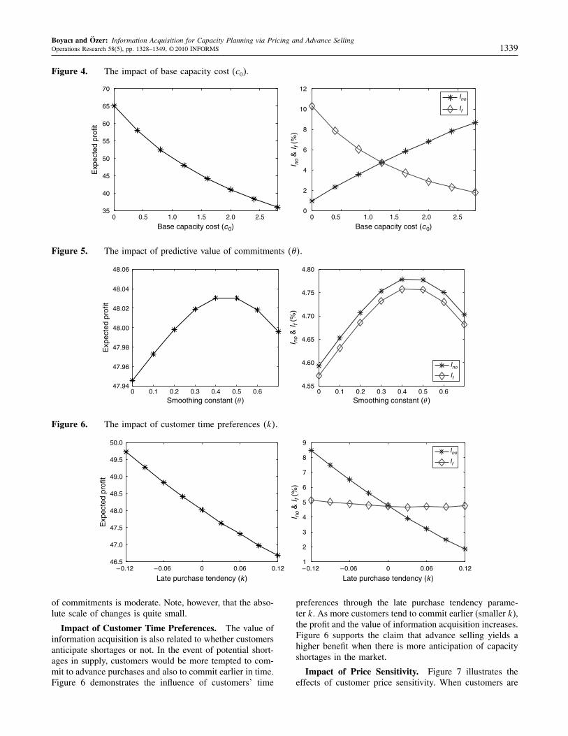
From the above results we conclude that the value of infor-mation acquisition is greater when time is not a major con-straint for the manufacturer in building capacity.Figure 4 illustrates the effects of base capacity cost
c0 (i.e., how expensive capacity cost is in general). Notethat the manufacturer’s profit naturally decreases as capac-ity becomes more costly, but the reduction in profits iseven higher when the manufacturer does not offer advancesales. Consequently, the benefit of advance selling actu-ally increases as base capacity cost increases. These resultsshow that the value of information acquisition is higherwhen capacity is more expensive relative to the penalty costof late construction.
Impact of Predictive Value of Commitments. Fig-ure 5 shows the impact of the predictive value of com-mitments, as measured by the smoothing parameter ��Observe that as � increases, the value of advance sellingfirst increases. However, when � is very high, the com-mitments send strong signals of future demand, indicatinga potential for high mean and variance. High uncertaintyreduces the expected profit, the value of information acqui-sition, as well as knowing when to stop. Consequently,advance selling is most beneficial when the predictive value
Boyacı and Özer: Information Acquisition for Capacity Planning via Pricing and Advance SellingOperations Research 58(5), pp. 1328–1349, © 2010 INFORMS 1339
Figure 4. The impact of base capacity cost (c0).
0 0.5 1.0 1.5 2.0 2.50
2
4
6
8
10
12
Base capacity cost (c0)
I no
& I f
(%
)
Ino
If
0 0.5 1.0 1.5 2.0 2.535
40
45
50
55
60
65
70
Base capacity cost (c0)
Exp
ecte
d pr
ofit
Figure 5. The impact of predictive value of commitments ���.
0 0.1 0.2 0.3 0.4 0.5 0.64.55
4.60
4.65
4.70
4.75
4.80
Smoothing constant (� )
I no
& I f
(%
)
Ino
If
0 0.1 0.2 0.3 0.4 0.5 0.647.94
47.96
47.98
48.00
48.02
48.04
48.06
Smoothing constant (� )
Exp
ecte
d pr
ofit
Figure 6. The impact of customer time preferences �k�.
–0.12 –0.06 0 0.06 0.121
2
3
4
5
6
7
8
9
Late purchase tendency (k )
I no
& I f
(%
)
Ino
If
–0.12 –0.06 0 0.06 0.1246.5
47.0
47.5
48.0
48.5
49.0
49.5
50.0
Late purchase tendency (k )
Exp
ecte
d pr
ofit
of commitments is moderate. Note, however, that the abso-lute scale of changes is quite small.
Impact of Customer Time Preferences. The value ofinformation acquisition is also related to whether customersanticipate shortages or not. In the event of potential short-ages in supply, customers would be more tempted to com-mit to advance purchases and also to commit earlier in time.Figure 6 demonstrates the influence of customers’ time
preferences through the late purchase tendency parame-ter k. As more customers tend to commit earlier (smaller k),the profit and the value of information acquisition increases.Figure 6 supports the claim that advance selling yields ahigher benefit when there is more anticipation of capacityshortages in the market.
Impact of Price Sensitivity. Figure 7 illustrates theeffects of customer price sensitivity. When customers are

Boyacı and Özer: Information Acquisition for Capacity Planning via Pricing and Advance Selling1340 Operations Research 58(5), pp. 1328–1349, © 2010 INFORMS
Figure 7. The impact of customer price sensitivity �b�.
1.4 1.6 1.8 2.0 2.2 2.4 2.60
2
4
6
8
10
12
Price sensitivity (b )
I no
& I f
(%
)
Ino
If
1.4 1.6 1.8 2.0 2.2 2.4 2.60
50
100
150
200
250
Price sensitivity (b )
Exp
ecte
d pr
ofit
more price concerned, the manufacturer’s profitability isreduced. This results in a lower value of information acqui-sition. Note also that when the customers are not price sen-sitive, acquiring information until the last period becomesmore likely. Hence the expected value of knowing when tostop advance selling decreases. These observations suggestthat low customer price sensitivity is another condition formaximizing the gains from advance selling.These numerical results help identify that advance selling
coupled with a let-them-come-and-build-it-later approach isa profitable strategy, in particular, when (i) demand uncer-tainty is high, (ii) more customers anticipate capacity short-ages in the market, (iii) building capacity is expensive buttiming is not a major concern, (iv) commitments have mod-erate predictive value about market potential, and (v) cus-tomer price sensitivity is relatively low. We note that, withthese conditions, one can construct cases where the valueof advance selling Ino is arbitrarily high.
6.5. Optimal Prices
To quantify the value of advance selling and the value ofknowing when to stop in the previous section, we compute,
Figure 8. Optimal advance selling and regular season prices.
1.0 1.5 2.0 2.5 3.0 3.5 4.07.8
8.0
8.2
8.4
8.6
8.8
9.0
9.2
9.4
9.6
9.8
Period (t)
Pric
es
pst
qt = 0.7�t
qt = �t
qt = 1.3�t
0 1 2 3 4 58.0
8.2
8.4
8.6
8.8
9.0
9.2
Cumulative commitment level
Pric
es
pc2
ps2
for each period, the optimal advance selling price pct and
the optimal regular season price pst when the manufacturer
decides to stop advance selling.Figure 8 plots the optimal prices as a function of commit-
ments qt for a given expected commitment level �t = 2�2when t = 2. The base data set is the same as in Figure 1.Note that the optimal market price ps
2 does not depend onthe commitments (Theorem 3). The optimal advance sellingprice pc
2, however, is increasing in the number of commit-ments. This is because having more commitments suggestsa stronger market and allows the manufacturer to chargehigher advance selling prices. Figure 8 also depicts theevolution of the prices over time for different commitmentlevels, qt = 0�7�t� qt = �t , qt = 1�3�t for each t� corre-sponding to low, medium, and high levels of commitment.For t = T = 5� the manufacturer is forced to build capacity.As before, for a given t� pc
t is nondecreasing in qt (highcommitments induce high advance sales prices). Further-more, both the advance sales prices and the regular sea-son prices are increasing over time. Finally, note that theadvance sales prices are always lower than the regular sea-son prices, implying that the customers committing to buyearlier are garnering discounts.

Boyacı and Özer: Information Acquisition for Capacity Planning via Pricing and Advance SellingOperations Research 58(5), pp. 1328–1349, © 2010 INFORMS 1341
Figure 9. Optimal advance sales prices as � changes for qt = 0�7�t� qt = �t , and qt = 1�3�t .
1 2 3 47.8
8.0
8.2
8.4
8.6
8.8
9.0
9.2
9.4
Period (t )
pc t
pc t
pc t
� = 0.06� = 0.1� = 0.14� = 0.18
1 2 3 47.8
8.0
8.2
8.4
8.6
8.8
9.0
Period (t )1 2 3 4
7.8
8.0
8.2
8.4
8.6
8.8
9.0
Period (t )
Figure 9 depicts the optimal advance sales prices as theincremental cost of building capacity � changes for differ-ent commitment levels qt = 0�7�t� qt = �t , and qt = 1�3�t .Note that for any given t where pc
t is not reported, itis optimal for the manufacturer to stop advance sellingin that period. It is possible to infer from Figure 9 thatfor any capacity cost structure, higher levels of commit-ment, induce the manufacturer to stop advance selling ear-lier. Generally speaking, increasing the incremental cost ofcapacity � results in higher advance selling prices. Theexceptions are due to discretization of the advance sellingprice set �t� which are set based on the optimal regu-lar season price ps
t � When � changes, so does the set ofadvance prices considered during that period, which canresult in nonmonotonic results. Consequently, the optimaladvance sales prices can display nonmonotonic behaviorover time as well (although within a fairly restricted range).We note that the changes in other cost or market parame-ters have rather predictable effects on optimal prices, andhence are omitted for brevity.
6.6. Computational Aspects, AlgorithmicalComplexity, and a Heuristic
In determining the optimal advance selling prices,we search n uniformly distributed prices in the range
Figure 10. The impact of price set �.
2 4 6 8 1047.70
47.75
47.80
47.85
47.90
47.95
48.00
48.05
48.10
Number of prices
Exp
ecte
d re
venu
e
a = 0.05
a = 0.1
a = 0.3
�1−a�pst � �1+a�ps
t � for each period t� Figure 10 illustratesthe optimal expected profit as a function of the number ofprices n and the price range a. We highlight two observa-tions. First, the expected profit increases with either factor.Essentially, increasing n and a is equivalent to relaxing theconstraint set, which in turn increases the optimal expectedprofit. Second, note that the marginal return on profit isdecreasing with these factors. For example, when a = 0�1considering seven or more prices does not change the profitsignificantly. Hence, there is a decreasing return to con-sidering larger price sets, which require significantly morecomputational effort.The algorithm to solve the general case is of complexity
O�nT �, which implies that finding optimal advance and reg-ular season prices is a computationally expensive task. Forthis reason we examined heuristic pricing policies. Recallthat ps
t is the optimal price for the regular sales season whenthe manufacturer stops collecting commitments at periodt. Consider a heuristic advance sales pricing policy underwhich the manufacturer charges the same price ps
t evenwhen she continues to collect commitments in period t�The computational effort required to numerically solve thisheuristic is the same as that of the exogenous pricing case(i.e., O�T �). We have tested the performance of this heuris-tic for different values of �, c0, and � and used regression tocompare the heuristic profit to the optimal profit (for detailsrefer to the electronic companion to this paper). The result-ing that R2 was close to 1 for all factors, suggesting thatthe heuristic can safely be used to investigate the impact ofparameter changes. The average optimality gap across allexperiments was also very small (0�535%).
7. Dynamic Pricing to Sell CapacityOur objective here is to investigate the tradeoff betweentwo strategies that mitigate the adverse effect of demanduncertainty: (1) information acquisition for capacity plan-ning through advance selling, and (2) revenue manage-ment of installed capacity through pricing during the regu-lar sales season. To do so, we study a manufacturer who,in addition to employing advance selling and pricing todetermine the capacity level, sets prices dynamically to sellthe installed capacity during the regular sales season. The

Boyacı and Özer: Information Acquisition for Capacity Planning via Pricing and Advance Selling1342 Operations Research 58(5), pp. 1328–1349, © 2010 INFORMS
manufacturer first acquires information through pricing andadvance selling. When it is optimal to do so, she stops col-lecting advance sales information and uses this informationto build capacity optimally. During the regular sales sea-son, the manufacturer sells the installed capacity throughdynamically setting prices. Note that this selling processcombines a strategic pricing and capacity decision withan operational pricing decision. Hence, the time scale andperiods for a strategic versus tactical level decision couldbe different. All actual sales and deliveries take place inthe regular sales season during which the manufacturer isallowed to adjust prices M times, M � 1.11
In order to solve this problem, we have to embed asecond-stage dynamic program that prescribes the optimaldynamic pricing policy and the resulting profit duringthe regular sales season for a given level of capac-ity and then determine the optimal capacity level. Sincethe manufacturer has M opportunities to adjust prices overthe regular sales season, let At�m� m = 1� � � � �M denote therandom market demand potential she will face in the mthpricing epoch (or subperiod). We assume that At�ms areindependently distributed IFR random variables with sup-port on 0���� Recalling that �t is the remaining demandpotential the manufacturer serves after stopping advanceselling, for logical consistency it is desirable that the dis-tribution of
∑Mm=1 At�m is the same as the distribution
of �t� Denoting the price charged in the mth epoch aspT �m, the random demand during the mth pricing epochis DT �m�pT �m � qt� �t� = ft�qt� �t�At�mp−b
T �m� Note that ouroriginal model corresponds to the case when M = 1� Fora given pricing policy � = �pT �1� � � � � pT �M�, the manufac-turer’s expected profit from remaining customers during theregular sales season is
�t�St� qt� �t ���
=M∑
m=1
�pT �m − cp�Emin�Sm�DT �m�pT �m � qt� �t���
− cu ESM − DT �m�pT �m � qt� �t��+
=M∑
m=1
pT �m Emin�Sm�DT �m�pT �m � qt� �t���
+ �cp − cu�ESM − DT �m�pT �m � qt� �t�� �+ − cpS1
= ft�qt� �t�
( M∑m=1
pT �m Emin�sm�At�mp−bT �m��
+ �cp − cu�EsM − At�mp−bT �M�+ − cps1
)
≡ ft�qt� �t� �t�st ����
where we define Sm ≡ St for m = 1� and Sm+1 =Sm − At�mp−b
T �m�+ for m > 1� and sm ≡ Sm/ft�qt� �t�. Thesecond equality holds because total sales during the reg-ular season plus the remaining capacity equals the totalcapacity at the beginning of regular sales season, i.e.,
S1 = ∑Mm=1 min�Sm�DT �m� + SM − DT �M�+� The objective
is to solve �t�st� = min�∈P �t�st � ��, where P denotes theset of all policies. Finding �t�st� involves solving the fol-lowing dynamic program:
�mt �sm� =max
pT �m
�pT �m Emin�sm�At�mp−bT �m��
+E �m+1t �sm − At�mp−b
T �m�+���
for 1�m < M� (19)
�Mt �sM� =max
pT �M
�pT �M Emin�sM�At�mp−bT �M��
+ �cp − cu�EsM − At�mp−bT �M�+�� (20)
where the expectation is with respect to the random variableAt�m in each period m� Notice that by definition �t�st� ≡� 1t �s1�.The manufacturer’s optimal net profit from remaining
customers when she stops advance selling in period t andsells the surplus capacity St via dynamic pricing is given by
ft�qt� �t�
[�t
(St
ft�qt� �t�
)− �ct + cp�
St
ft�qt� �t�
]
= ft�qt� �t� �t�st� − �ct + cp�st�
= ft�qt� �t� � 1t �s1� − �ct + cp�s1��
Optimizing over the capacity level also, the manufacturer’soptimal net profit from remaining customers becomes
�∗t �qt� �t� = ft�qt� �t� �t�s
∗t � − �ct + cp�s∗
t �
= ft�qt� �t� � 1t �s∗
1� − �ct + cp�s∗1 �� (21)
Defining � ∗t ≡ �t�s
∗t �− �ct +cp�s∗
t � we have a similar struc-ture as in Equation (3), i.e., �∗
t �qt� �t� = ft�qt� �t��∗t � This
implies that all of the preceding results regarding the opti-mal stopping policy for acquiring advance sales informationhold with the profit �∗
t �qt� �t� replaced by its new defini-tion above. We formalize this in the next theorem, whichwe state without proof.
Theorem 6. When the manufacturer sells installed capac-ity by dynamically adjusting prices, the optimal stoppingpolicy for advance selling is a state-dependent control-bandpolicy.
The above result establishes the structure of the opti-mal policy. Yet, computing policy parameters, such as theoptimal prices and thresholds, remains a difficult task.Essentially, the problem is a two-stage, nested, stochasticdynamic program with multiple decision epochs and con-tinuous, multidimensional state spaces. The first stage isthe optimal stopping problem whose solution depends onthe second-stage dynamic program specified in Equations(19)–(20). Even this second-stage problem is a challengingone to solve numerically. Monahan et al. (2004) study a

Boyacı and Özer: Information Acquisition for Capacity Planning via Pricing and Advance SellingOperations Research 58(5), pp. 1328–1349, © 2010 INFORMS 1343
Figure 11. Multiple pricing opportunities to sell capacity during the regular sales season.
1 2 3 4 5 6 764.4
64.6
64.8
65.0
65.2
65.4
65.6
65.8
66.0
M
Exp
ecte
d pr
ofit
1 2 3 4 5 6 74.0
4.5
5.0
5.5
M
I no
& I f
(%
)
Ino
If
similar problem as the second-stage DP and report that effi-cient results can only be obtained when cp = cu� For thiscase, they show that �m
t �sm� = r∗m�sm�n� where
r∗m =max
z
z −Ez − At�m�+ + r∗m+1E�z − At�m�+�n
zn�
s∗1 =
(nr∗
1
ct + cp
)b
�
�t�s∗t � − �ct + cp�s∗
t = 1− n
n�ct + cp�
(nr∗
1
ct + cp
)b
�
where n = 1 − 1/b and r∗M+1 = 0. Hence, �∗
t �qt� �t� =ft�qt� �t��
∗t � where � ∗
t = �1− n�/n�nr∗1 /ct + cp�b.
We use this result to numerically solve the second-stagedynamic program and embed its solution to the optimalstopping problem and solve for the optimal advance salesprices and stopping thresholds. Figure 11 illustrates theresults of a numerical study in which At�m is normally dis-tributed with same mean and variance across all m. Theparameters of this example are the same as the base set,except � = 40 and � = 0�2�Three observations are worth noting. First note that the
expected profit is increasing with the number of pricingopportunities. The percentage increase in expected profitbetween having M = 7 pricing epochs to having oneis 1�25% = �65�83 − 65�02�/65�02. Second, the marginalincrease in profit is decreasing. Third, the expected valueof advance selling is decreasing, but the marginal decreaseis also decreasing. This observation suggests that dynamicpricing during the regular sales season is only a partial sub-stitute for dynamic pricing during advance sales periods.Altogether, these observations suggest that using a smallnumber of price adjustments or even a single price dur-ing the regular sales season is reasonably close to optimal,considering also the fact that such price adjustments arecostly due to transaction costs (e.g., due to advertising newprices). Similar observations for this second-stage problemare also reported in Gallego and van Ryzin (1994).
8. Summary and DiscussionIn this paper, we study the strategy of obtaining informationabout market potential through advance sales for a bettercapacity decision. In particular, we consider a manufacturerwho collects revenue and information through advance sell-ing prior to building capacity. Using advance sales infor-mation, the manufacturer sets the capacity and satisfies theremaining demand during the regular season as much aspossible, subject to the available capacity. We establish theoptimal pricing strategy both for the advance and regu-lar selling seasons and the optimal capacity to build. Wealso establish the optimality of a control-band policy thatprescribes when to stop collecting advance sales informa-tion. This policy is also optimal when prices are set exoge-nously (e.g., as mark-up or mark-down schedules). Througha numerical study, we quantify the expected value of thiscapacity planning strategy under different market and oper-ating conditions. We show that advance selling coupledwith a let-them-come-and-build-it-later approach is a prof-itable strategy, in particular, when (i) demand uncertaintyis high, (ii) more customers anticipate capacity shortages inthe market, (iii) building capacity is expensive but timingis not a major concern, (iv) commitments have moderatepredictive value about market potential, and (v) customerprice sensitivity is relatively low. We also show that theextreme strategy of collecting full advance selling informa-tion or not collecting any information leads to inferior solu-tions in comparison to the optimal pricing strategy. Theseresults suggest that the practice of advance selling is ofmost value for, e.g., high technology, apparel, and phar-maceutical industries. For example, telecommunication andsemiconductor industries face high capacity building costs.They often introduce new products for which the marketuncertainty is also high relative to commodity type prod-ucts. Finally, we study a scenario in which the manufacturercontinues to sell installed capacity through dynamic pric-ing. Modeling this scenario bridges the revenue and capac-ity management literatures. We show that selling capacityby dynamically adjusting regular sales prices increases the

Boyacı and Özer: Information Acquisition for Capacity Planning via Pricing and Advance Selling1344 Operations Research 58(5), pp. 1328–1349, © 2010 INFORMS
expected profit but only to a limited extent. Next, we revisita few aspects of our framework.
Other Market Signal Functions. In our numericalexamples we have utilized a specific form of the mar-ket signal function, which smoothed the predictive valueof cumulative commitments over time. As noted earlier,it is possible to envision a case where next period’sexpected market signal is the same as the current level(i.e., Eft+1�qt+1� �t+1�� = ft�qt� �t�) for any selected pricept . In other words, the evolution of the market signal isa martingale. This would correspond to an extreme casewhere the current market signal is a firm indicator of futuredemand, such that the manufacturer expects the current sig-nal to sustain regardless of the price charged. As an exam-ple, consider the following scenario where the manufacturertracks the value ft of the market signal itself and recur-sively updates it:
ft = �1− ��ft−1 + �dt−1
E�t−1�p−bt−1
= �1− ��ft−1 + �ft−1
�t−1
E�t−1�� (22)
In this case, the manufacturer needs to know only ft toupdate the market signal and the cumulative commitmentsqt , to determine its profit and optimal course of action. Thisdoes not suggest, however, that ft is independent of theqt� As a matter of fact, substituting qt − qt−1 for dt andaccordingly taking �t = �ft−1� qt−1� pt−1�, Equation (22)can be stated equivalently as ft�qt� �t� = �1−��ft−1 +��qt −qt−1�/�E�t−1�pt−1
−b�� which is a linear increasingfunction of cumulative commitments qt . Also, at time zero,Eft�qt� �t�� = 1 for any given t and price path. Hence,our structural results on the form of the optimal policy foracquiring advance sales information apply to this martingaleevolution model as well.It is also possible to envision a case where the mar-
ket signal depends only on the cumulative commitmentsqt and not on past prices or other historical informa-tion. In this case, the linear increasing signal ft�qt� wouldmodel strictly the “word-of-mouth effect” created by thecumulative number of early purchasers. This type of depen-dency of future demand on past sales is a common fea-ture in new product diffusion models (as in Bass 1969).This case may occur when the manufacturer announces theprices privately to each potential customer without reveal-ing historical information. Residential real estate developerssometimes use such a selling strategy. Alternatively, such amarket signal function could approximately model a casewhere early customers are relatively insensitive to prices.Our structural results in §§4 and 5 would apply to thiscase as well, with the added simplification that the optimalcontrol-band policies would be state independent.
Connection with Demand Learning Models. Althoughthere is no formal learning of demand parameters in ourdemand model, the functional form of the market signalmakes it applicable to a class of Bayesian models. Bayesianmodels of demand learning involve a multiple period hori-zon whereby the demand in each period follows a knowndistribution with an unknown parameter or vector of param-eters (say, �). There is a known prior distribution of �,which is updated on the basis of a sufficient statistic �t astime progresses and demand realizes. For a certain class ofa conjugate family of distributions, �t is cumulative pastsales qt or a function of it, and its effect on the demanddistribution can be factored out as a scaling function inthe same spirit as our market signal function ft� · � · ��This approach was first used by Scarf (1960) to solve thedynamic inventory management problem efficiently, and itwas later extended by Azoury (1985). Next we providesome specific examples to illustrate the applicability of ourframework and results in this setting. We refer the reader toAzoury (1985) for a full account of the required conditions,details, and other examples.Suppose that the market demand potential in each
period �t are independent with distribution �t = kt�, wherekts �
∑Tt=1 kt = 1� are known scalars. Consider the case
kt = 1/T and an exogenous, fixed pricing scheme pt = pfor t = 1� � � � � T � This implies the demands across peri-ods are independent and distributed identically. When thedistribution belongs to the Gamma family with unknownscale parameter � that also has a Gamma prior distribu-tion, cumulative sales qt is the sufficient statistic for updat-ing demand (hence �t = � for all t). Furthermore, theBayes estimate of demand in period t can be written asft�qt�Dt , where ft�qt� = a + qt and a > 0 is a knownconstant, and the distribution of Dt only depends on t(Scarf 1960, Azoury 1985). Notice that ft�qt� is increas-ing linear in qt . Consequently, our optimal policy resultsin §4 apply to this scenario. When kt and pt are noniden-tical (but still exogenous), defining k′
t = ktp−bt , we have
�t = k′t�, which are independent but no longer identically
distributed. In this case, qt is no longer a sufficient statistic;it is necessary to know the history of past demand real-izations (hence qts), causing a significant increase in thedimensionality of the state space.12 When prices are deci-sion variables, it becomes necessary to track past pricesthat define the scalars k′
t . Nevertheless, given the history ofpast prices and commitments, the scaling function can beexpressed as a linear function of qt , which implies that ourstate-dependent optimal policy results apply. The details aredeferred to the electronic companion to this paper.
Other Price Functions. In a multiplicative demandenvironment, there are alternatives to the iso-elastic pricefunction d�p� = p−b. This form facilitates the derivation ofunique optimal regular sales prices ps
t in Theorem 3. Asshown in Song et al. (2008), the uniqueness is guaranteedwhen the curvature of d�p�� given as d�p��d′′�p�/d′�p�2��
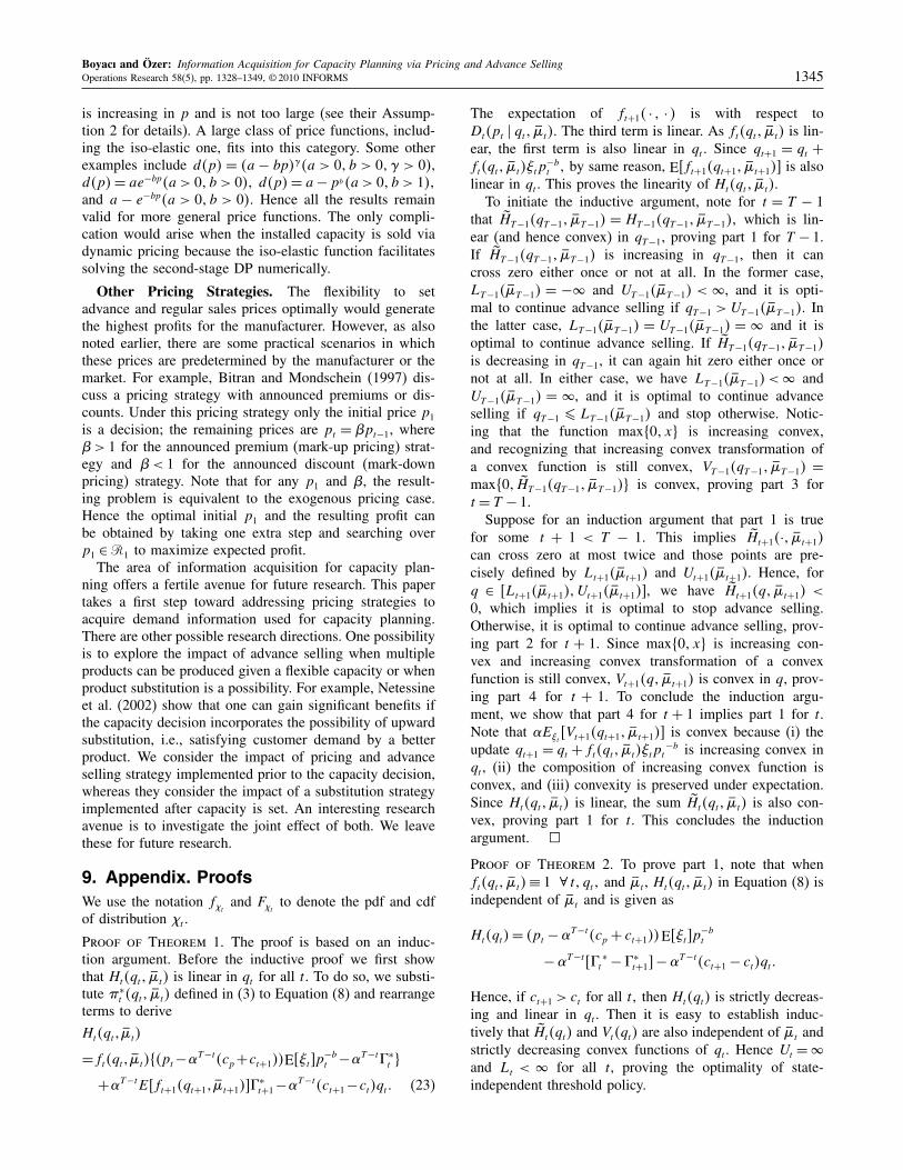
Boyacı and Özer: Information Acquisition for Capacity Planning via Pricing and Advance SellingOperations Research 58(5), pp. 1328–1349, © 2010 INFORMS 1345
is increasing in p and is not too large (see their Assump-tion 2 for details). A large class of price functions, includ-ing the iso-elastic one, fits into this category. Some otherexamples include d�p� = �a − bp���a > 0� b > 0� � > 0�,d�p� = ae−bp�a > 0� b > 0�� d�p� = a − pb �a > 0� b > 1��and a − e−bp�a > 0� b > 0�� Hence all the results remainvalid for more general price functions. The only compli-cation would arise when the installed capacity is sold viadynamic pricing because the iso-elastic function facilitatessolving the second-stage DP numerically.
Other Pricing Strategies. The flexibility to setadvance and regular sales prices optimally would generatethe highest profits for the manufacturer. However, as alsonoted earlier, there are some practical scenarios in whichthese prices are predetermined by the manufacturer or themarket. For example, Bitran and Mondschein (1997) dis-cuss a pricing strategy with announced premiums or dis-counts. Under this pricing strategy only the initial price p1
is a decision; the remaining prices are pt = �pt−1, where� > 1 for the announced premium (mark-up pricing) strat-egy and � < 1 for the announced discount (mark-downpricing) strategy. Note that for any p1 and �, the result-ing problem is equivalent to the exogenous pricing case.Hence the optimal initial p1 and the resulting profit canbe obtained by taking one extra step and searching overp1 ∈�1 to maximize expected profit.The area of information acquisition for capacity plan-
ning offers a fertile avenue for future research. This papertakes a first step toward addressing pricing strategies toacquire demand information used for capacity planning.There are other possible research directions. One possibilityis to explore the impact of advance selling when multipleproducts can be produced given a flexible capacity or whenproduct substitution is a possibility. For example, Netessineet al. (2002) show that one can gain significant benefits ifthe capacity decision incorporates the possibility of upwardsubstitution, i.e., satisfying customer demand by a betterproduct. We consider the impact of pricing and advanceselling strategy implemented prior to the capacity decision,whereas they consider the impact of a substitution strategyimplemented after capacity is set. An interesting researchavenue is to investigate the joint effect of both. We leavethese for future research.
9. Appendix. ProofsWe use the notation f�t
and F�tto denote the pdf and cdf
of distribution �t�
Proof of Theorem 1. The proof is based on an induc-tion argument. Before the inductive proof we first showthat Ht�qt� �t� is linear in qt for all t� To do so, we substi-tute �∗
t �qt� �t� defined in (3) to Equation (8) and rearrangeterms to derive
Ht�qt� �t�
=ft�qt� �t���pt −�T −t�cp +ct+1��E�t�p−bt −�T −t� ∗
t �
+�T −tEft+1�qt+1� �t+1���∗t+1−�T −t�ct+1−ct�qt� (23)
The expectation of ft+1� · � · � is with respect toDt�pt � qt� �t�. The third term is linear. As ft�qt� �t� is lin-ear, the first term is also linear in qt� Since qt+1 = qt +ft�qt� �t��tp
−bt � by same reason, Eft+1�qt+1� �t+1�� is also
linear in qt . This proves the linearity of Ht�qt� �t�.To initiate the inductive argument, note for t = T − 1
that HT −1�qT −1� �T −1� = HT −1�qT −1� �T −1�� which is lin-ear (and hence convex) in qT −1, proving part 1 for T − 1.If HT −1�qT −1� �T −1� is increasing in qT −1, then it cancross zero either once or not at all. In the former case,LT −1� �T −1� = −� and UT −1� �T −1� < �, and it is opti-mal to continue advance selling if qT −1 > UT −1� �T −1�� Inthe latter case, LT −1� �T −1� = UT −1� �T −1� = � and it isoptimal to continue advance selling. If HT −1�qT −1� �T −1�is decreasing in qT −1, it can again hit zero either once ornot at all. In either case, we have LT −1� �T −1� < � andUT −1� �T −1� = �, and it is optimal to continue advanceselling if qT −1 � LT −1� �T −1� and stop otherwise. Notic-ing that the function max�0� x� is increasing convex,and recognizing that increasing convex transformation ofa convex function is still convex, VT −1�qT −1� �T −1� =max�0� HT −1�qT −1� �T −1�� is convex, proving part 3 fort = T − 1.Suppose for an induction argument that part 1 is true
for some t + 1 < T − 1� This implies Ht+1�·� �t+1�can cross zero at most twice and those points are pre-cisely defined by Lt+1� �t+1� and Ut+1� �t+1�. Hence, forq ∈ Lt+1� �t+1��Ut+1� �t+1��, we have Ht+1�q� �t+1� <0, which implies it is optimal to stop advance selling.Otherwise, it is optimal to continue advance selling, prov-ing part 2 for t + 1. Since max�0� x� is increasing con-vex and increasing convex transformation of a convexfunction is still convex, Vt+1�q� �t+1� is convex in q, prov-ing part 4 for t + 1. To conclude the induction argu-ment, we show that part 4 for t + 1 implies part 1 for t.Note that �E�t
Vt+1�qt+1� �t+1�� is convex because (i) theupdate qt+1 = qt + ft�qt� �t��tpt
−b is increasing convex inqt , (ii) the composition of increasing convex function isconvex, and (iii) convexity is preserved under expectation.Since Ht�qt� �t� is linear, the sum Ht�qt� �t� is also con-vex, proving part 1 for t. This concludes the inductionargument. �
Proof of Theorem 2. To prove part 1, note that whenft�qt� �t� ≡ 1 ∀ t� qt� and �t , Ht�qt� �t� in Equation (8) isindependent of �t and is given as
Ht�qt� = �pt − �T −t�cp + ct+1��E�t�p−bt
− �T −t�t∗ − � ∗
t+1� − �T −t�ct+1 − ct�qt�
Hence, if ct+1 > ct for all t� then Ht�qt� is strictly decreas-ing and linear in qt . Then it is easy to establish induc-tively that Ht�qt� and Vt�qt� are also independent of �t andstrictly decreasing convex functions of qt . Hence Ut = �and Lt < � for all t, proving the optimality of state-independent threshold policy.

Boyacı and Özer: Information Acquisition for Capacity Planning via Pricing and Advance Selling1346 Operations Research 58(5), pp. 1328–1349, © 2010 INFORMS
When ct+1 = ct ∀ t� the last term in Ht�qt� also drops.Consequently, Ht�qt�, Ht�qt� and Vt�qt� are all indepen-dent of qt and equal constants Ht , Ht , and Vt , respectively.Then it is easy to verify that the optimal stopping time foracquiring advance sales information is the first t ∈ 1� T �such that Ht = 0�
To prove part 2, recall from Theorem 1 and its proof thatthe structure of the policy is driven by Ht�qt� �t� given inEquation (23), which is linear in qt . For any t, �t , and ct ,for a sufficiently large ct+1� the term in � · � is decreasingbecause � ∗
t , defined in (3), does not depend on ct+1. Thesecond term is also decreasing in qt because � ∗
t+1 is neg-ative for large ct+1 (the higher the cost of building capac-ity, the lower will be optimal profit from remaining cus-tomers), while Eft+1�qt+1� �t+1�� does not depend on ct+1.The last terms are clearly decreasing. As a result, Ht�qt� �t�is decreasing in qt . This means that when ct+1 is suffi-ciently larger than ct�, Ht�qt� �t� would be decreasing inqt� Next, one can establish inductively that Ht�qt� �t� andVt�qt� �t� are decreasing convex functions of qt becausethis property is preserved under max�0� f �x�� operator.Hence, Ut� �t� = � for all t, proving the optimality of state-dependent threshold policy. �
Proof of Theorem 3. Let pt denote the selling seasonprice set in period t, and ps
t is optimal value. Clearly, pst
maximizes �t�pt� St � qt� �t� defined in (2) over pt� Substi-tuting yt ≡ St/�ft�qt� �t�� in (2), we get
�t�pt� St � qt� �t� = ft�qt� �t��t�pt� yt�� where
�t�pt� yt� = ��pt − cp − ct�yt
− �pt − cp + cu�Eyt − �tp−bt �+��
(24)
Hence, maximizing (2) for a given commitment qt and his-tory �t boils down to maximizing (24). Recall that sinceIFR property is closed under convolutions (Barlow andProschan 1975), �t is also IFR, meaning its failure rateht�x� = f�t
�x�/�1− F�t�x�� is increasing. Since �t is IFR,
it also has increasing generalized failure rate (IGFR), i.e.,xht�x� is also increasing (Lariviere and Porteus 2001).Song et al. (2008) study the optimal ordering and pricing
problem for a newsvendor with order-up-to level y, retailprice p� purchase cost w, and salvage value b (p > w >b � 0). They establish (in Theorem 1) the existence of aunique optimal �y∗� p∗� pair under multiplicative demandfor a large class of demand functions that includes theiso-elastic function when the distribution of the underlyinguncertainty is IGFR. They derive the optimal pair �y∗� p∗�sequentially, i.e., they first determine the unique optimalprice p�y� for a given y and then derive the unique opti-mal y∗ and resulting p∗� Observe that (24) is equivalent tothe standard newsvendor function with p = pt , w = cp +ct ,and b = cp − cu. Hence, their result applies as long as pt >cp + ct > cp − cu � 0� Note that the second inequality isimmediately satisfied. Consequently, when cp � cu and thefirst inequality holds, (24) has a unique optimal �y∗
t � pst ��
Next we show that the first inequality is true for a candidateoptimal stocking level and price pair and hence the pair isalso the unique maximizer.To do so, it is convenient to conduct the stocking factor
transformation (Petruzzi and Dada 1999) zt = yt/p−bt and
hence write (24) equivalently as
�t�pt� zt� = p−bt ��pt − cp − ct�zt
− �pt − cp + cu�Ezt − �t�+�� (25)
For a fixed zt , taking the derivative of (25), we obtain aftersome manipulation
��t�pt� zt�
�pt
= �b − 1�p−�b+1�t �zt −Ezt − �t�
+�
·{
b
b − 1
(cp + ctzt + cu Ezt − �t�
+
zt −Ezt − �t�+
)−pt
}� (26)
Setting the derivative to zero and solving for pt yields theunique optimal price
pt�zt� =(
b
b − 1
)(cp + ctzt + cu Ezt − �t�
+
zt −Ezt − �t�+
)
as in (11) because pt�zt� > cp + ct for all zt � 0. Substitut-ing pt�zt� in (25) results in
�t�zt� = �t�pt�zt�� zt�
= 1b
pt�zt�−�b−1��zt −Ezt − �t�
+�� (27)
Taking the derivative of (27) we get
��t�zt�
�zt
=pt�zt�−b�1−F�t
�zt��
{�pt�zt�−cp +cu�−
ct +cu
1−F�t�zt�
}�
Hence z∗t is the unique solution of �pt�zt� − cp + cu� −
�ct + cu�/�1 − F�t�zt�� = 0 as stated in the theorem, and
pst = pt�z
∗t �.
By definition S∗t = ft�qt� �t�z
∗t �p
st �
−b, so that Q∗t =
qt +S∗t � Substituting z∗
t in (27) results in � ∗t given by (12)
and �∗t �qt� �t� = ft�qt� �t��
∗t � Hence, �∗
t �qt� �t� =�t�p
st � S∗
t � qt� �t� = ∑t−1k=1 pkdk − �cp + ct�qt +
ft�qt� �t��∗t � �
Proof of Theorem 4. Note that pst > cp + ct follows
directly from (11) in Theorem 3, since b/�b − 1� > 1 andzt/�zt − Ezt − �t�
+� > 1� In order to prove the remainingresults, it is convenient to change the order of optimizationof the profit function �t�pt� zt� given by (25). Suppose thatpt is fixed. Let zt�pt� denote the corresponding optimalstocking factor, which is given uniquely by the equation
P��t > zt� = ct + cu
pt − cp + cu
� (28)

Boyacı and Özer: Information Acquisition for Capacity Planning via Pricing and Advance SellingOperations Research 58(5), pp. 1328–1349, © 2010 INFORMS 1347
Substituting zt�pt� into �t�pt� zt�, we can write
��t�pt� zt�pt��
�pt
= ��t�pt� zt�
�pt
+ ��t�pt� zt�
�zt
�zt
�pt
at zt = zt�pt�� Noting that the second term in���t�pt� zt�pt���/�pt equals zero at zt = zt�pt�� it followsfrom (26) that the optimal price ps
t is given as the uniquesolution to(
b
b−1
){cp + ctzt�pt�+cuEzt�pt�−�t�
+
zt�pt�−Ezt�pt�−�t�+
}−pt =0� (29)
Furthermore, for pt < pst , the left-hand side of (29) is
positive and for pt > pst , it is negative.
We first characterize the change in the optimal stock-ing factor (28) and then the resulting change in (29). Thisenables us to prove the impact on optimal price ps
t . Fromthe joint effect, we can then establish the effect on opti-mal capacity level Q∗
t = qt + ft�qt� �t�z∗t �p
st �
−b. The prooffor each cost element (cp� ct� cu) follows identical logicand intermediate steps. For this reason, in order to avoidrepetition, we provide a detailed proof for only one ofthem, namely the production cost cp� Taking derivativeswith respect to cp, for a fixed pt , we have �zt�pt�/�cp =−�ct + cu/��pt − cp + cu�
2f�t�zt�pt��� < 0� Let
O�pt� = cp + ctzt�pt� + cuEzt�pt� − �t�+
zt�pt� − Ezt�pt� − �t�+ �
Note from (29) that pst is increasing in cp if �O�pt�/
�cp > 0�
�O�pt�
�cp
=1+�ct +cu�zt�pt�F�t
�zt�pt��−Ezt�pt�−�t�+
�zt�pt�−Ezt�pt�−�t�+�2
�zt�pt�
�cp
�
=1−(
ct +cu
pt −cp +cu
)2 zt�pt�F�t�zt�pt��−Ezt�pt�−�t�
+
f�t�zt�pt���zt�pt�−Ezt�pt�−�t�
+�2�
=1− �1−F�t�zt�pt���
2
f�t�zt�pt��
zt�pt�F�t�zt�pt��−Ezt�pt�−�t�
+
�zt�pt�−Ezt�pt�−�t�+�2
�
The last equality is from (28). Notice that
�1− F�t�zt�pt���
2
f�t�zt�pt��
zt�pt�F�t�zt�pt�� − Ezt�pt� − �t�
+
�zt�pt� − Ezt�pt� − �t�+�2
<�1− F�t
�zt�pt���2
f�t�zt�pt��
F�t�zt�pt��
zt�pt� − Ezt�pt� − �t�+
< 1− F�t�zt�pt�� < 1�
The first inequality is evident. The second one is obtainedby bounding the function zt − Ezt − �t�
+ using the factthat �t is IFR. In particular,
zt −Ezt −�t�+ =
∫ zt
0�1−F�t
�u��du��1−F�t
�zt��
f�t�zt�
F�t�zt��
Consequently, �O�pt�/�cp > 0� and hence pst is increasing
in cp� With this result, using implicit differentiation on (29),it is easy to verify that �ps
t /�cp > 1� which immediatelyimplies (from (28)) that �z∗
t /�cp < 0� Since pst is increasing
and z∗t is decreasing, Q∗
t is decreasing in cp. �
Proof of Theorem 5. Similar to the proof of Theorem 1,first note that Ht�pt� qt� �t� in Equation (15) is linearin qt for a given pt and �t . The rest of the proof isbased on an induction argument. For t = T − 1, notethat RT −1�pT −1� q� �T −1� = HT −1�pT −1� q� �T −1� whichis linear in q, proving part 1 for T − 1. This impliesthat if HT −1�pT −1� q� �T −1� is increasing (resp., decreas-ing) in q then RT −1�pT −1� q� �T −1� is also increasing(resp., decreasing) in q. Next we show that this impliesHT −1�q� �T −1� is also increasing (resp., decreasing) in q.Define q1 < q2 and let p1 ≡ argmaxp RT −1�p� q1� �T −1�and p2 ≡ argmaxp RT −1�p� q2� �T −1�. When RT −1�p� q�
�T −1� is decreasing in q, we have HT −1�q2� �T −1� =RT −1�p2� q2� �T −1� < RT −1�p2� q1� �T −1� < RT −1�p1� q1��T −1� = HT −1�q1� �T −1�. Hence, HT −1�q� �T −1� is alsodecreasing in q. When RT −1�p� q� �T −1� is increasingin q, we have HT −1�q1� �T −1� = RT −1�p1� q1� �T −1� <RT −1�p1� q2� �T −1� < RT −1�p2� q2� �T −1� = HT −1�q2��T −1�. Hence HT −1�q� �T −1� is also increasing in q. Thisimplies parts 3 and 4 for T − 1 along the same argumentsas in the proof of Theorem 1.Next, suppose for an induction argument that Part 1 is
true for t. This implies part 2 because convexity is pre-served under maximization (Porteus 2002, p. 226). Hence,given �t
Ht�q� �t� can cross zero at most twice, and thosepoints are given precisely as Lt� �t� and Ut� �t�� From con-vexity, it follows also that Ht�q� �t� � 0 on Lt� �t� � q �
Ut� �t�, in which case it is optimal to stop advance selling.Otherwise, it is optimal to continue advance selling, prov-ing part 3. Noting that the function max�0� x� is increasingconvex, and increasing convex transformation of a con-vex function is still convex, Vt�q� �t� =max�0� Ht�q� �t��is also convex, proving part 4 for t. To complete theproof, we show that part 4 for t implies part 1 for t − 1.Note that qt = qt−1 + ft−1�qt−1� �t−1��t−1p
∗t−1
−b is linearincreasing in qt−1� Hence, �EVt�qt� �t�� is also convex inqt−1. Since Ht−1�pt−1� qt−1� �t−1� is linear in qt−1, the sumRt−1�pt−1� qt−1� �t−1� is also convex in qt−1, proving part 1for t − 1 and concluding the induction argument. �
10. Electronic CompanionAn electronic companion to this paper is available as partof the online version that can be found at http://or.journal.informs.org/.
Endnotes1. During September 2002, Christer Lundberg from Eric-sson presented an advance selling strategy for long rangeforecasting during the Ericsson Supply Chain AcademyConference in Sweden.

Boyacı and Özer: Information Acquisition for Capacity Planning via Pricing and Advance Selling1348 Operations Research 58(5), pp. 1328–1349, © 2010 INFORMS
2. This information could be the vector of past prices pt ≡�p1� � � � � pt−1� offered up until that period or some functionof them. It could also include any other relevant informa-tion excluding qt .3. Linear increasing means that higher commitments signalthe potential for stronger future demand. For example,Carlson (1983) studies apparel sales data of a departmentstore and shows that given the regular and mark-downprices, the post-mark-down sales rate is a linear functionof the pre-mark-down sales rate. Some Bayesian learningmodels satisfy this assumption as well.4. Note that Eft�qt� �t�� can be equal to any constant.Without loss of generality, we take the constant to be 1.5. Similarly, its expected value Eft+1�qt+1� �t+1�� taken attime t can be higher than, lower than, or equal to ft�qt� �t�.This models a scenario where the current market signal isonly a partial determinant of (expected) future demand. Inthe more extreme case, Eft+1�qt+1� �t+1�� = ft�qt� �t� forany price pt , which models a scenario where the predictivevalue of the current market signal is very strong. In thiscase the manufacturer expects the current signal to sustainat the same level, regardless of the price charged.6. The specification of � · � depends on the definition of�t . For example, it may not be necessary to know both pt
and dt to update �t .7. The manufacturer can also ensure positive return fromadvance purchasers by requiring prices to be such that pt �
cp +maxt=1� ���� T �ct� for all t� This assumption, however, isnot required for our analysis.8. A constant � implies that the discount factor is station-ary over time and the length of the periods are not toodifferent. Otherwise, period-specific discount factors �t canbe used.9. We remark that the optimal policy remains as a control-band when predictive value is very strong, i.e., when expec-tation Eft+1�qt+1� �t+1�� taken at time period t equalsft�qt� �t� for any price path.10. Note that the market signal can also be expressed recur-sively, i.e.,
ft+1�qt+1� �t+1� = ft�qt� �t� + ��tp−bt �ft�qt� �t��t − qt��
We observe that when qt > �t (which implies ft�qt� �t�> 1), the next period’s expected market signal Eft+1�qt+1��t+1�� is still larger than 1 but is less than ft�qt� �t�. Hence,although the manufacturer has sold more than she initiallyexpected, she does not necessarily expect the future demandto arrive at exactly the same strength. In other words, thereis smoothing of the advance sales information provided bythe market signal function, the extent of which is deter-mined by �� The opposite scenario qt < �t can be inter-preted similarly.11. An alternative way to model is to assume that the man-ufacturer can change prices in periods t + 1� � � � � T wheret is the stopping time. Our structural results remain validunder this model as well.
12. The sufficient statistics is �t =∑t−1j=1�dj/k′
j �, where dj
is the realized demand in period j� and the scaling func-tion is given as k′
t�a + �t�� Since dj = qj+1 − qj� taking�t = �q1� � � � � qj−1�� �t and hence the scaling function canbe stated equivalently as a linear increasing function of qt�
AcknowledgmentsThe authors thank the anonymous associate editor andreviewers, Yigal Gerchak, Warren Hausman, Hau Lee, andRobert Phillips. They appreciate the helpful and construc-tive comments of participants of the following sessions: the2002 INFORMS annual meeting in San Jose; the Septem-ber 2002 presentation at Ericsson, Stockholm, Sweden;the 2004 MSOM Conference in the Netherlands; the 2005International Colloquium for GERAD’s 25th Anniversaryin Montreal; and colloquiums at Columbia University andStanford University. The authors also thank Sechan Oh forhis help with the numerical study. Özalp Özer gratefullyacknowledges initial financial support from Ericsson. Thelisting of authors is alphabetical.
ReferencesAngelus, A., E. Porteus. 2002. Simultaneous capacity and production man-
agement of short-life-cycle, produce-to-stock goods under stochasticdemand. Management Sci. 48(3) 399–413.
Araman, V., R. Caldentey. 2009. Dynamic pricing for nonperishable prod-ucts with demand learning. Oper. Res. 57(5) 1169–1188.
Aviv, Y., A. Federgruen. 1997. Stochastic inventory models with lim-ited production capacity and periodically varying parameters. Probab.Engrg. Inform. Sci. 11(1) 107–135.
Aviv, Y., A. Pazgal. 2005a. A partially observed Markov decision processfor dynamic pricing. Management Sci. 51(9) 1400–1416.
Aviv, Y., A. Pazgal. 2005b. Pricing of short life-cycle products throughactive learning. Working paper, Washington University in St. Louis.
Azoury, K. S. 1985. Bayes solution to dynamic inventory models underunknown demand distribution. Management Sci. 31(9) 1150–1160.
Barlow, R. E., F. Proschan. 1975. Statistical Theory of Reliability and LifeTesting: Probability Models. Holt, Rinehart, and Winston, Inc., NewYork.
Bass, F. M. 1969. A new product growth model for consumer durables.Management Sci. 15(5) 215–227.
Bitran, G. R., R. Caldentey. 2003. An overview of pricing models forrevenue management. Manufacturing Service Oper. Management 5(3)203–229.
Bitran, G. R., S. V. Mondschein. 1997. Periodic pricing of seasonal prod-ucts in retailing. Management Sci. 43(1) 64–79.
Braden, D., S. Oren. 1994. Nonlinear pricing to produce information.Marketing Sci. 13(3) 310–326.
Bradley, J. R., P. W. Glynn. 2002. Managing capacity and inventory jointlyin manufacturing systems. Management Sci. 48 273–288.
Cachon, G. 2004. The allocation of inventory risk in a supply chain:Push, pull, and advance-purchase discount contracts. ManagementSci. 50(2) 222–238.
Carlson, P. G. 1983. Fashion retailing: The sensitivity of rate of sale tomark-down. J. Retailing 59 67–76.
Carr, S., W. Lovejoy. 2000. The inverse newsvendor problem: Choosingan optimal demand portfolio for capacitated resources. ManagementSci. 46(7) 912–927.
Chen, F. 2001. Market segmentation, advanced demand information, andsupply chain performance. Manufacturing Service Oper. Management3(1) 53–67.

Boyacı and Özer: Information Acquisition for Capacity Planning via Pricing and Advance SellingOperations Research 58(5), pp. 1328–1349, © 2010 INFORMS 1349
Dana, J. 1998. Advanced purchase discounts and price discrimination incompetitive markets, J. Political Econom. 395–422.
Dixit, A., R. Pindyck. 1994. Investment Under Uncertainty. PrincetonUniversity Press, Princeton, NJ.
Dong, L., K. Zhu. 2007. Two-wholesale-price contracts: Push, pull, andadvance-purchase discount contracts. Manufacturing Service Oper.Management 9(3) 291–311.
Elmaghraby, W., P. Keskinocak. 2003. Dynamic pricing in the presence ofinventory considerations: Research overview, current practices, andfuture directions. Management Sci. 49(10) 1287–1309.
Feng, Y., G. Gallego. 1995. Optimal starting times for end-of-season salesand optimal stopping times for promotional fares. Management Sci.41(8) 1371–1391.
Fisher, M., A. Raman. 1996. Reducing the cost of demand uncertaintythrough accurate response in early sales. Oper. Res. 44(1) 87–99.
Fraiman, N., M. Singh. 2002. Zara. Teaching case, Columbia BusinessSchool, New York.
Gallego, G., Ö. Özer. 2001. Integrating replenishment decisions withadvance demand information. Management Sci. 47(10) 1344–1360.
Gallego, G., G. van Ryzin. 1994. Optimal dynamic pricing of inventorieswith stochastic demand over finite horizons. Management Sci. 40(8)999–1019.
Gayon, J. P., S. Benjaafar, F. de Véricourt. 2009. Using imperfectdemand information in production-inventory systems with multiplecustomer classes. Manufacturing Service Oper. Management. 11(1)128–143.
Hu, X., I. Duenyas, R. Kapuscinski. 2004. Advance demand informationand safety capacity as a hedge against demand and capacity uncer-tainty. Working paper, University of Michigan, Ann Arbor.
Lariviere, M. A., E. L. Porteus. 2001. Selling to a newsvendor: An analysisof price-only contracts. Manufacturing Service Oper. Management3(4) 293–305.
Lovejoy, W., Y. Li. 2002. Hospital operating room capacity expansion.Management Sci. 48(11) 1369–1387.
Luss, H. 1982. Operations research and capacity expansion problems: Asurvey. Oper. Res. 30(5) 907–947.
Manne, S. A. 1967. Investments for Capacity Expansion: Size, Locationand Time-Phasing. Allen & Unwin, London.
Monahan, G. E., N. C. Petruzzi, W. Zhao. 2004. The dynamic pricingproblem from a newsvendor’s perspective. Manufacturing ServiceOper. Management 6(1) 73–91.
Neslin, S. A., S. G. Powell, L. S. Stone. 1995. The effect of retailer andconsumer response on optimal manufacturer advertising and tradepromotion strategies. Management Sci. 41(5) 749–766.
Netessine, S., N. Rudi. 2006. Supply chain choice on the Internet. Man-agement Sci. 52(6) 844–864.
Netessine, S., G. Dobson, R. Shumsky. 2002. Flexible service capacity:Optimal investment and the impact of demand correlation. Oper. Res.50(2) 375–388.
Özer, Ö., W. Wei. 2004. Inventory control with limited capacity andadvance demand information. Oper. Res. 52(6) 988–1000.
Özer, Ö., O. Uncu, W. Wei. 2007. Selling to the “newsvendor” with aforecast update: Analysis of a dual purchase contract. Eur. J. Oper.Res. 182(3) 1150–1176.
Petruzzi, N. C., M. Dada. 1999. Pricing and the newsvendor problem: Areview with extensions. Oper. Res. 47(2) 183–194.
Phillips, R. 2005. Pricing and Revenue Optimization. Stanford UniversityPress, Stanford, CA.
Porteus, E. L. 2002. Foundations of Stochastic Inventory Theory. StanfordUniversity Press, Stanford, CA, 226.
Prasad, A., K. E. Stecke, X. Zhao. 2010. Advance selling by a newsvendorretailer. Production Oper. Management. Forthcoming.
Scarf, H. 1960. Some remarks on Bayes solutions to the inventory prob-lem. Naval Res. Logist. Quart. 14 591–596.
Song, Y., S. Ray, S. Li. 2008. Structural properties of buyback contractsfor price-setting newsvendors. Manufacturing Service Oper. Manage-ment 10(1) 1–18.
Talluri, K., G. J. van Ryzin. 2004. The Theory and Practice of RevenueManagement. Springer, New York.
Taylor, T. 2006. Sale timing in a supply chain: When to sell to the retailer.Manufacturing Service Oper. Management 8(1) 23–42.
Van Mieghem, J. A. 2003. Capacity management, investment, and hedg-ing: Review and recent developments. Manufacturing Service Oper.Management 5(4) 269–302.
Wang, T., L. B. Toktay. 2008. Inventory management with advancedemand information and flexible delivery. Management Sci. 54(4)716–732.
Weng, Z. K., M. Parlar. 1999. Integrating early sales with productiondecisions: Analysis and insights. IIE Trans. 31(11) 1051–1060.
Xie, J., S. M. Shugan. 2001. Electronic tickets, smart cards, and onlineprepayments: When and how to advance sell. Marketing Sci. 20(3)219–243.

OPERATIONS RESEARCHdoi 10.1287/opre.1100.0798ec
informs ®
© 2010 INFORMS
e - c o m p a n i o nONLY AVAILABLE IN ELECTRONIC FORM
Electronic Companion—“Information Acquisition for Capacity Planning viaPricing and Advance Selling: When to Stop and Act?” by Tamer Boyacı and
Özalp Özer, Operations Research, doi 10.1287/opre.1100.0798.

An Electronic Companion to
“Information Acquisition for Capacity Planning via Pricing and
Advance Selling: When to Stop and Act?”
Tamer Boyaci and Ozalp Ozer
Operations Research
Performance of the Heuristic Pricing Policy
We test the performance of this heuristic by comparing the resulting expected profit to that of
optimal pricing policy. To do so, we test nine settings for each δ, c0 and σ and report the resulting
profits and the optimality gap ε in Table 1. Let Gh be the optimal expected profit under the heuristic
pricing strategy. We use regression to compare Gh to the optimal profit G∗ and report the R2.
δ G∗ Gh ε(%) c0 G∗ Gh ε(%) σ G∗ Gh ε(%)0.18 50.852 50.490 0.713 0 65.061 64.827 0.360 30 49.120 48.921 0.4050.21 49.977 49.642 0.670 0.4 58.088 57.807 0.483 40 48.900 48.684 0.4400.24 49.223 48.896 0.664 0.8 52.527 52.250 0.529 50 48.68 48.477 0.4150.27 48.587 48.275 0.642 1.2 48.019 47.738 0.586 60 48.459 48.210 0.5130.30 48.019 47.738 0.586 1.6 44.270 43.988 0.637 70 48.218 47.973 0.5080.33 47.518 47.265 0.533 2.0 41.068 40.818 0.609 80 48.019 47.738 0.5860.36 47.087 46.853 0.497 2.4 38.362 38.106 0.664 90 47.801 47.505 0.6190.39 46.714 46.493 0.472 2.8 35.986 35.762 0.624 100 47.557 47.276 0.5920.42 46.379 46.171 0.449 3.2 33.938 33.704 0.690 110 47.344 47.050 0.620R2 = 99.99%, c0 = 2, σ = 80 R2 = 100%, δ = 0.03, σ = 80 R2 = 99.95%, δ = 0.03, c0 = 2
Table 1: Performance of the heuristic pricing policy
Connection with Demand Learning Models
Consider the following demand learning setting which is suitable to our decision problem and frame-
work. The market demand potential in each period is given as ξt ≡ ktξ for t = 1, ..., T, where ξ’s
in each period are iid, k′ts are known scalars, and hence ξt are independent random variables. One
practical way to interpret this setup is to think of ξ as the total random market size and kt the
fraction of customers who potentially buy in period t (in this case it makes sense to have∑kt = 1).
Let dt(pt) denote the deterministic price function, which captures the effects of prices. Although any
40

function can be used, to be able to make parallels with our framework, suppose that dt(pt) = p−bt .
As a result, the distribution of demand in each period is given as dt(pt)ξt ≡ dt(pt)ktξ ≡ mt(pt)ξ.
Suppose that the distribution of ξ is unknown but belongs to a gamma distribution with unknown
scale parameter ω. The density of ξ for a fixed value of ω is: φ(z|ω) = ωλzλ−1e−ωz
Γ(λ) , λ > 0, z ≥ 0.
Suppose that the scale parameter ω itself has a gamma prior distribution g(ω) = baωa−1e−bω
Γ(a) , a, b >
0, ω ≥ 0, and the firm updates its information in a Bayesian manner over time as demand realizes.
Let dt denote the realized demand in period t. It is well-known from Scarf (1960) and Azoury
(1985) that the sufficient statistic St for updating the demand distribution is St =∑t−1
j=1dj
mj(pj).
Furthermore, the Bayesian estimate (i.e., posterior distribution) of demand in period t has density
φt(d|St) =Γ(a+ λt)(b+ St)a+λ(t−1)(d/mt(pt))λ−1
mt(pt)Γ(λ)Γ(a+ λ(t− 1))(b+ St + d/mt(pt))a+λt.
Furthermore, φt(d|St) = 1ϕt(St)ψt(d/ϕt(St)), where ϕt(St) = mt(pt)(b + St) and ψt(u) = (Γ(a +
λt)uλ−1)/(Γ(λ)Γ(a + λ(t − 1))(1 + u)a+λt). The above states that ϕt(St) is a function that scales
random demand. Let Dt(pt|St) denote the random demand each period given the sufficient statistic
St. We have
Dt(pt|St) = ϕt(St)Dt = mt(pt)(b+ St)Dt, (30)
where the distribution of Dt (given by ψt(u)) only depends on t. If the firm decides to stop ad-
vance selling in period t, then there is no more learning, so the demand distribution does not get
updated. For any given selling season price p, the remaining demand in the market is Xt(p|St) =∑Tj=tDj(p|St) = (b+ St)
∑Tj=tmj(p)Dj , where Dj ’s are iid with distribution given by ψt(u).
The demand function in (30) is consistent with our market signal based demand framework.
In particular, the function (b + St) is akin to our market signal function ft(qt, µt). In fact, since
qt =∑t−1j=1 dj, we can write St as a function of qt and define ft(qt, µt) accordingly. This would require
the knowledge of the entire past sequence of dj for j = 1, .., t−1. Hence the history µt would contain
qj and pj for j = 1, ...t − 1, (hence mj(pj) will also be known). 14 This follows because S1 = 0,
S2 = q2m1(p1) , . . . , St = qt
mt−1(pt−1) +∑t−2i=1 qt−i
(1
mt−i−1(pt−i−1) −1
mt−i(pt−i)
)for t ≥ 2. Consequently,
for t = 1, q1 ≡ 0, µ1 ≡ ∅, f1(q1, µ1) ≡ 1, and for t ≥ 2, we have ft(qt, µt)
ft(qt, µt) = b+qt
mt−1(pt−1)+
t−2∑i=1
qt−i
(1
mt−i−1(pt−i−1)− 1mt−i(pt−i)
)(31)
14Note that state space reduction is possible if the manufacturer tracks the value ft of the market signal itself. In
this case, the manufacturer would need (ft,dt, pt) to update the market signal and qt to determine the profit and the
optimal course of action.
41

Observe that ft(qt, µt) is linear increasing in qt given the history µt. Hence the demand function given
by (30) can be equivalently stated as Dt(pt|qt, µt) = ft(qt, µt)p−bt(ktDt
), which is has the same form
as our demand model. Furthermore, when the firm stops advance selling in period t, the remaining
demand can be stated as Xt(pt|qt, µt) = ft(qt, µt)p−bt∑Tj=t
(kjDj
). Defining χt ≡
∑Tj=t
(kjDj
), we
have, as in our framework Xt(pt|qt, µt) = ft(qt, µt)p−bt χt.
42