Influence of solar variability on the - Hvar...
29
Transcript of Influence of solar variability on the - Hvar...

Influence of solar variability on the Earth’s climate requires knowledge of
1. Short-‐ and long-‐term solar variability 2. Solar-‐terrestrial interac8ons 3. Mechanisms determining the response of the Earth’s climate
system to these interac8ons Rind, 2002

Mechanisms of solar influences on climate
Kodera & Kuroda , 2002
Solar activity modulates cosmic rays
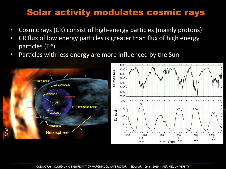
• Cosmic rays (CR) consist of high-‐energy par8cles (mainly protons) • CR flux of low energy par8cles is greater than flux of high energy
par8cles (E-‐γ) • Par8cles with less energy are more influenced by the Sun
NAS
A

Cosmic ray flux on Earth depends on
• Solar magne8c field and Solar wind • Geomagne8c field (ver8cal cutoff rigidity) • Earth’s atmosphere
CR showers (cascade) → ioniza8on in the atmosphere

Houghton et al., 1996
Earth’s radiative balance and clouds

“Clear-air” mechanism
Laken & Čalogović, 2015, TOSCA handbook
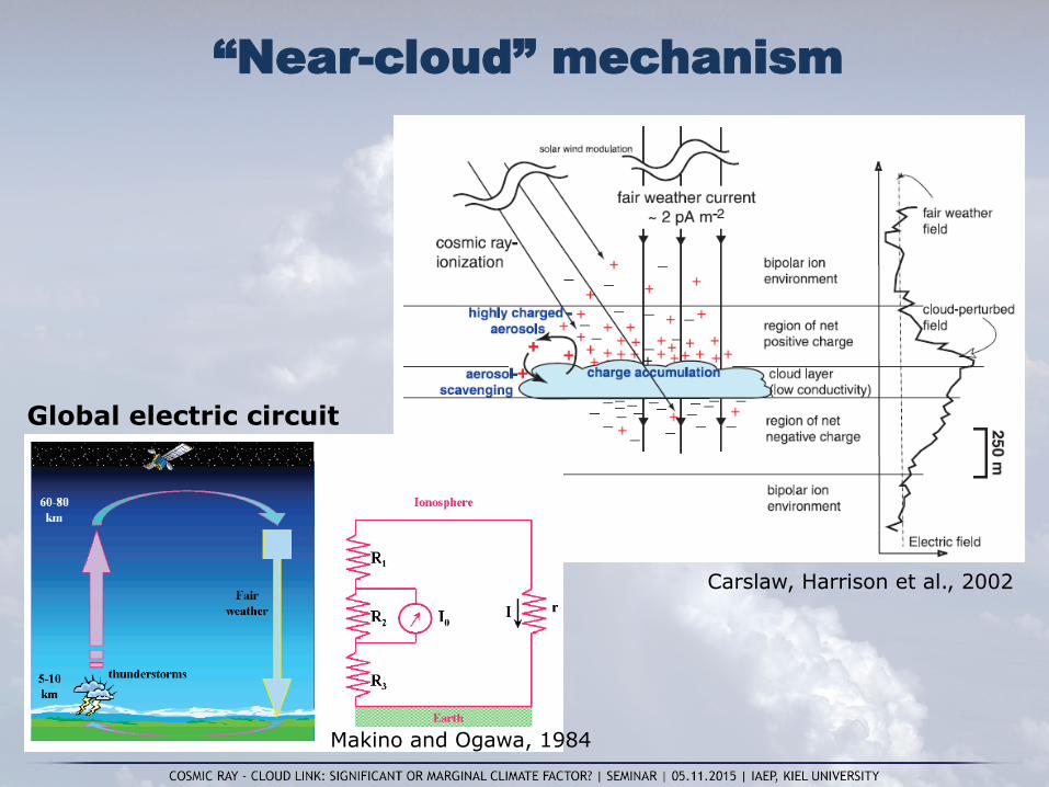
“Near-cloud” mechanism
Global electric circuit
Carslaw, Harrison et al., 2002
Makino and Ogawa, 1984
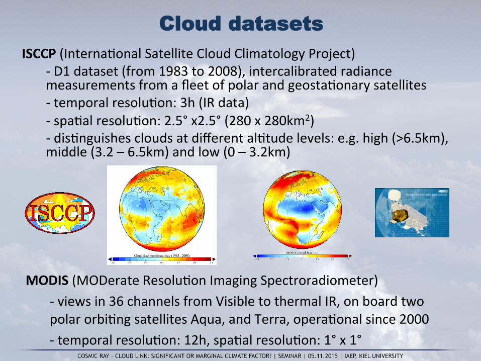
Cloud datasets ISCCP (Interna8onal Satellite Cloud Climatology Project)
-‐ D1 dataset (from 1983 to 2008), intercalibrated radiance measurements from a fleet of polar and geosta8onary satellites -‐ temporal resolu8on: 3h (IR data) -‐ spa8al resolu8on: 2.5° x2.5° (280 x 280km2) -‐ dis8nguishes clouds at different al8tude levels: e.g. high (>6.5km), middle (3.2 – 6.5km) and low (0 – 3.2km)
MODIS (MODerate Resolu8on Imaging Spectroradiometer) -‐ views in 36 channels from Visible to thermal IR, on board two polar orbi8ng satellites Aqua, and Terra, opera8onal since 2000 -‐ temporal resolu8on: 12h, spa8al resolu8on: 1° x 1°
The hypothesized link between cosmic ray flux and cloud cover
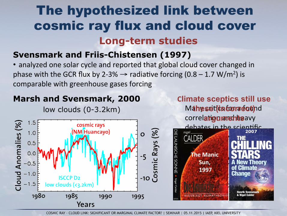
Svensmark and Friis-Chistensen (1997) • analyzed one solar cycle and reported that global cloud cover changed in phase with the GCR flux by 2-‐3% → radia8ve forcing (0.8 – 1.7 W/m2) is comparable with greenhouse gases forcing
Marsh and Svensmark, 2000 low clouds (0-3.2km)
Long-term studies
Many cri8cs for a found correla8on and heavy debates in the scien8fic community: e.g. Kernthaler et al., 1999 Sun & Bradley, 2002; Laut, 2003; Kristjansson et al., 2002; 2003; Sloan and Wolfendale, 2008…
The Manic Sun, 1997
Climate sceptics still use these (incorrect)
arguments
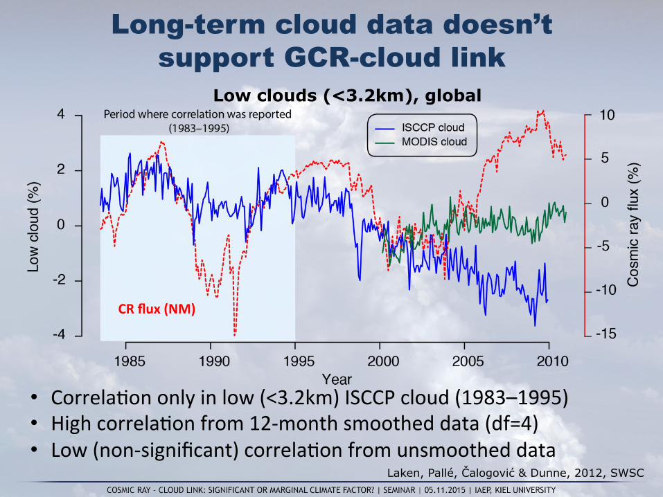
Long-term cloud data doesn’t support GCR-cloud link
Laken, Pallé, Čalogović & Dunne, 2012, SWSC
• Correla8on only in low (<3.2km) ISCCP cloud (1983–1995) • High correla8on from 12-‐month smoothed data (df=4) • Low (non-‐significant) correla8on from unsmoothed data
Low clouds (<3.2km), global
CR flux (NM)

Artificial anti-correlation exists between low and high/middle troposphere cloud
• Low cloud obscured by overlying cloud (measurements are non-‐cloud penetra8ng).
• Number of geosta8onary satellites increased over 8me → ar8ficial drop in low cloud
• Errors in iden8fying cloud height can contribute to shios between low and high cloud.
• Satellite cloud issues well known: e.g. Hughes, 1984; Minnis, 1989, Tian & Curry, 1989; Rozendall et al. 1995; Loeb & Davies, 1996; Salby & Callaghan, 1997, Campbell, 2004
Evidence for CR – cloud link is based on low level clouds:
these data are not reliable!
Lake
n, P
allé
, Čal
ogov
ić &
Dun
ne,
2012
, SW
SC
Many addi=onal problems of long-‐term analysis (e.g. ENSO, volcanic erup=ons...)
changes in the satellite constella8on
Laken, Pallé, Čalogović i Dunne, 2012, SWSC
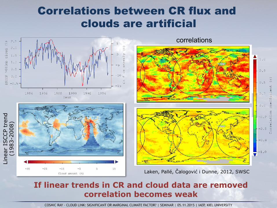
If linear trends in CR and cloud data are removed correlation becomes weak
Correlations between CR flux and clouds are artificial
Line
ar I
SCCP
tren
d (1
983-
2008
)
correlations

Timeline of geostationary satellite operation at equator over ISCCP observation period
Cloud data should not be used for long-‐term analysis (Stubenrauch et al. 2012, 2013)
from: NOAA/NCDC, satellite data, ISCCP resource
Beginning of measurements
20 years later
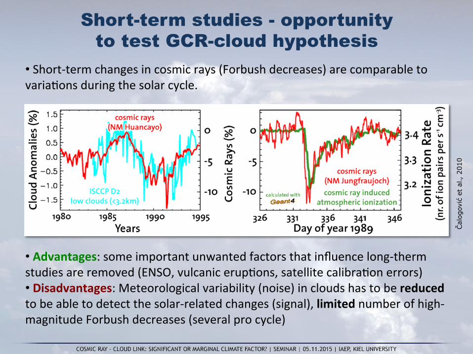
Short-term studies - opportunity to test GCR-cloud hypothesis
• Short-‐term changes in cosmic rays (Forbush decreases) are comparable to varia8ons during the solar cycle.
• Advantages: some important unwanted factors that influence long-‐therm studies are removed (ENSO, vulcanic erup8ons, satellite calibra8on errors) • Disadvantages: Meteorological variability (noise) in clouds has to be reduced to be able to detect the solar-‐related changes (signal), limited number of high-‐magnitude Forbush decreases (several pro cycle)
Čal
ogov
ić e
t al
., 20
10
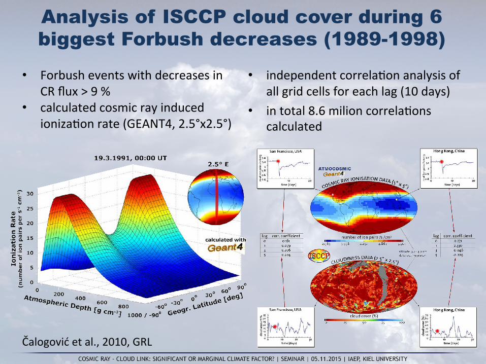
Analysis of ISCCP cloud cover during 6 biggest Forbush decreases (1989-1998)
Čalogović et al., 2010, GRL
• Forbush events with decreases in CR flux > 9 %
• calculated cosmic ray induced ioniza8on rate (GEANT4, 2.5°x2.5°)
• independent correla8on analysis of all grid cells for each lag (10 days)
• in total 8.6 milion correla8ons calculated
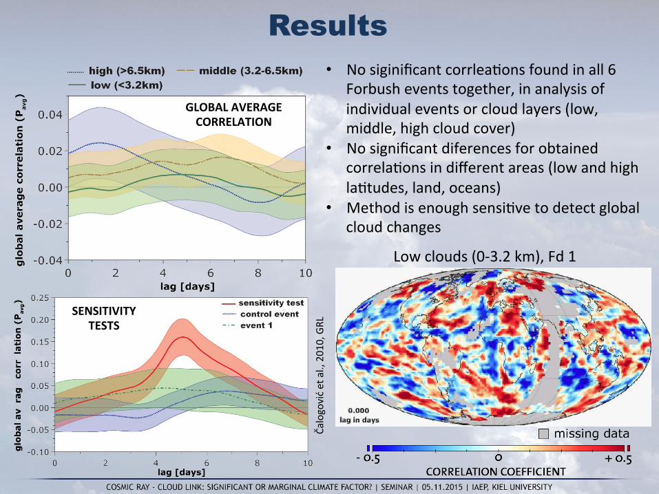
Results
Čalogović et al., 201
0, GRL
Low clouds (0-‐3.2 km), Fd 1
• No siginificant corrlea8ons found in all 6 Forbush events together, in analysis of individual events or cloud layers (low, middle, high cloud cover)
• No significant diferences for obtained correla8ons in different areas (low and high la8tudes, land, oceans)
• Method is enough sensi8ve to detect global cloud changes
GLOBAL AVERAGE CORRELATION
SENSITIVITY TESTS
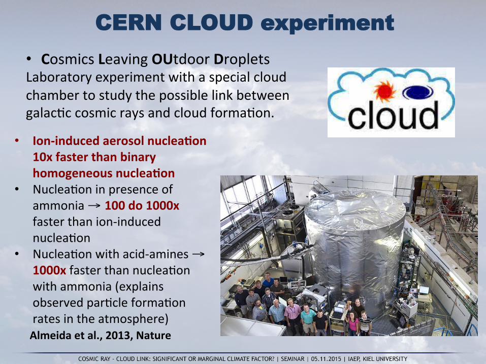
• Cosmics Leaving OUtdoor Droplets Laboratory experiment with a special cloud chamber to study the possible link between galac8c cosmic rays and cloud forma8on.
CERN CLOUD experiment
• Ion-‐induced aerosol nuclea=on 10x faster than binary homogeneous nuclea=on
• Nuclea8on in presence of ammonia → 100 do 1000x faster than ion-‐induced nuclea8on
• Nuclea8on with acid-‐amines → 1000x faster than nuclea8on with ammonia (explains observed par8cle forma8on rates in the atmosphere)
Almeida et al., 2013, Nature
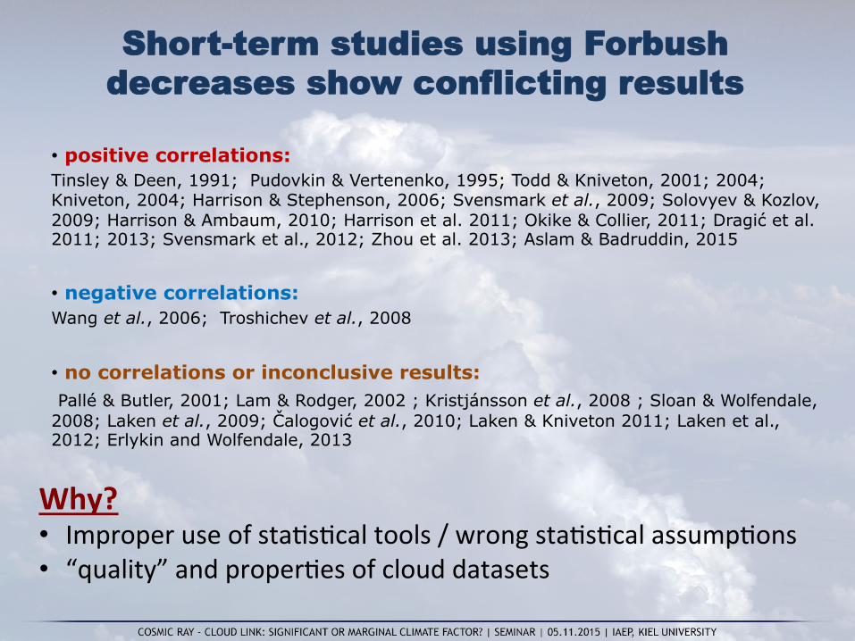
Short-term studies using Forbush decreases show conflicting results
• positive correlations: Tinsley & Deen, 1991; Pudovkin & Vertenenko, 1995; Todd & Kniveton, 2001; 2004; Kniveton, 2004; Harrison & Stephenson, 2006; Svensmark et al., 2009; Solovyev & Kozlov, 2009; Harrison & Ambaum, 2010; Harrison et al. 2011; Okike & Collier, 2011; Dragić et al. 2011; 2013; Svensmark et al., 2012; Zhou et al. 2013; Aslam & Badruddin, 2015 • negative correlations: Wang et al., 2006; Troshichev et al., 2008 • no correlations or inconclusive results: Pallé & Butler, 2001; Lam & Rodger, 2002 ; Kristjánsson et al., 2008 ; Sloan & Wolfendale, 2008; Laken et al., 2009; Čalogović et al., 2010; Laken & Kniveton 2011; Laken et al., 2012; Erlykin and Wolfendale, 2013
Why? • Improper use of sta8s8cal tools / wrong sta8s8cal assump8ons • “quality” and proper8es of cloud datasets
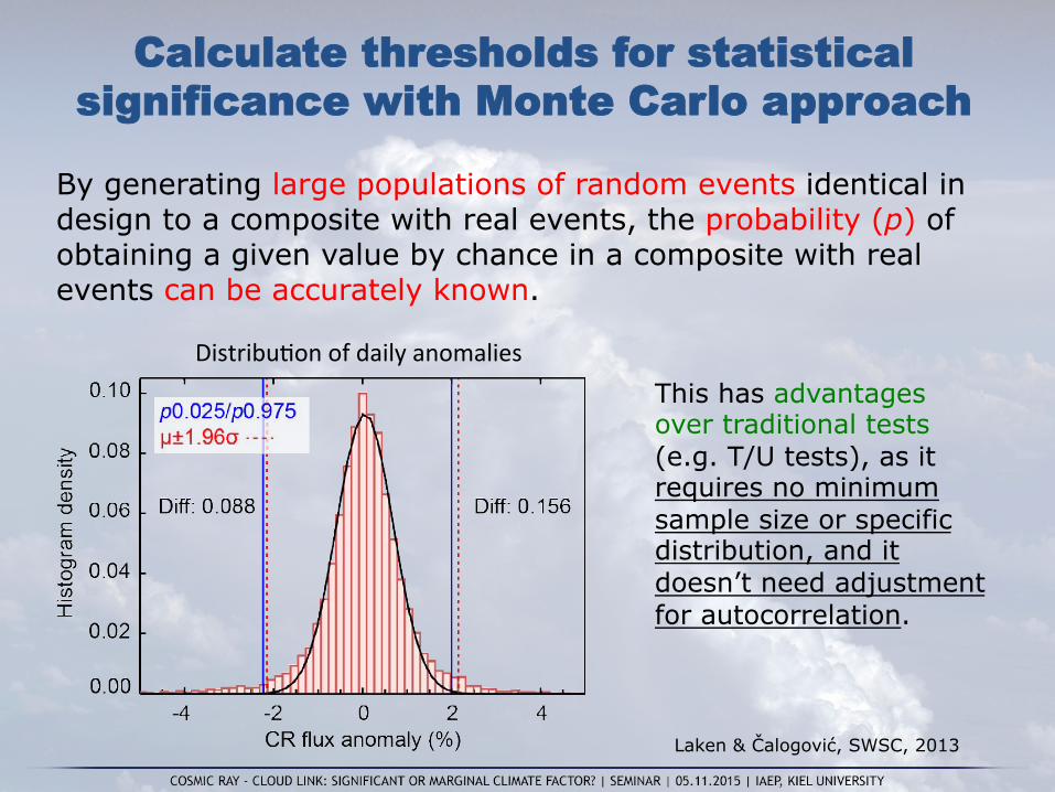
Calculate thresholds for statistical significance with Monte Carlo approach
By generating large populations of random events identical in design to a composite with real events, the probability (p) of obtaining a given value by chance in a composite with real events can be accurately known.
Distribu8on of daily anomalies This has advantages over traditional tests (e.g. T/U tests), as it requires no minimum sample size or specific distribution, and it doesn’t need adjustment for autocorrelation.
Laken & Čalogović, SWSC, 2013
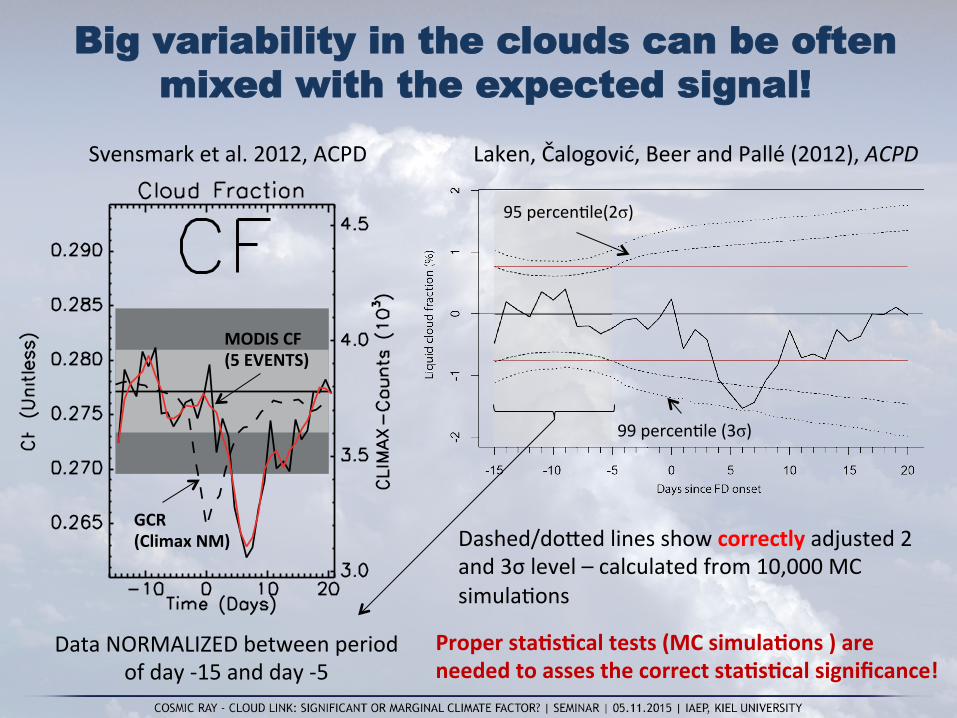
Big variability in the clouds can be often mixed with the expected signal!
Svensmark et al. 2012, ACPD
Data NORMALIZED between period of day -‐15 and day -‐5
GCR (Climax NM)
MODIS CF (5 EVENTS)
Laken, Čalogović, Beer and Pallé (2012), ACPD
Dashed/dowed lines show correctly adjusted 2 and 3σ level – calculated from 10,000 MC simula8ons
95 percen8le(2σ)
99 percen8le (3σ)
Proper sta=s=cal tests (MC simula=ons ) are needed to asses the correct sta=s=cal significance!

Extension to longer analysis periods reveals no unusual variability in clouds during Fd events
Laken, Čalogović, Beer and Pallé (2012), ACPD
±20 day analysis period
MODIS Liquid cloud frac8on changes using 5 biggest Fd events from Svensmark et al. (2012)
±100 day analysis period
Values are anomalies from 21-‐day moving averages (i.e. mean of each day subtracted from 21-‐day moving average). Dashed and dowed lines indicate the 95th and 99th (two-‐tailed) percen8le confidence intervals respec8vely calculated from 100,000 Monte Carlo simula8ons.
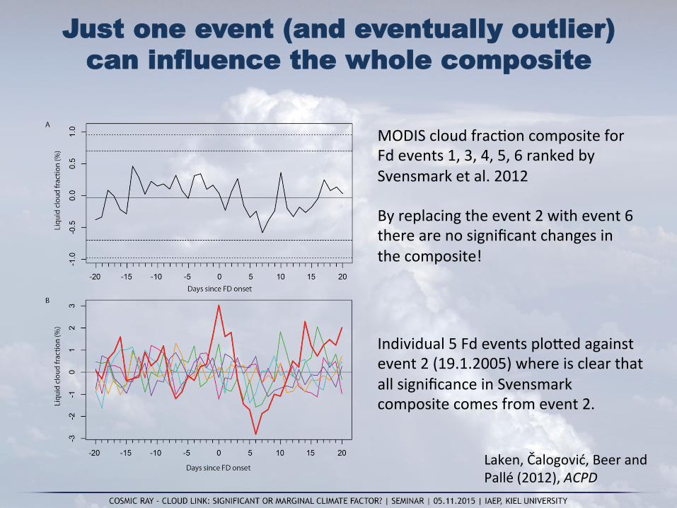
Just one event (and eventually outlier) can influence the whole composite
Laken, Čalogović, Beer and Pallé (2012), ACPD
MODIS cloud frac8on composite for Fd events 1, 3, 4, 5, 6 ranked by Svensmark et al. 2012
By replacing the event 2 with event 6 there are no significant changes in the composite!
Individual 5 Fd events plowed against event 2 (19.1.2005) where is clear that all significance in Svensmark composite comes from event 2.

DTR shows response to Fd events?
• Dragić et al. (2011) uses composite of 37 Fd events (>7%) that show significant increase in DTR → support for GCR-‐cloud hypothesis
• Surface level Diurnal Temperature Range (DTR) → effec8ve proxy for cloud cover (indirect cloud data)
• DTR has longer 8me span than satellite cloud observa8ons → allows to use the larger number of Forbush events

Analysis of Dragić et al. (2011) results
Analysis of the same data as in Dragic et al. (DTR data and 37 Forbush events) shows that authors didn’t es8mate correctly sta8s8cal significance using t-‐test and certain sta8s8cal assump8ons. Significance intervals calculated from
100 000 Monte Carlo simula8ons (using 21-‐day running average)
Dragić et al. Normaliza8on of data in period from t-‐10 to t-‐5 and 99% significance intervals
Laken, Čalogović, Shahbaz and Pallé (2012), JGR
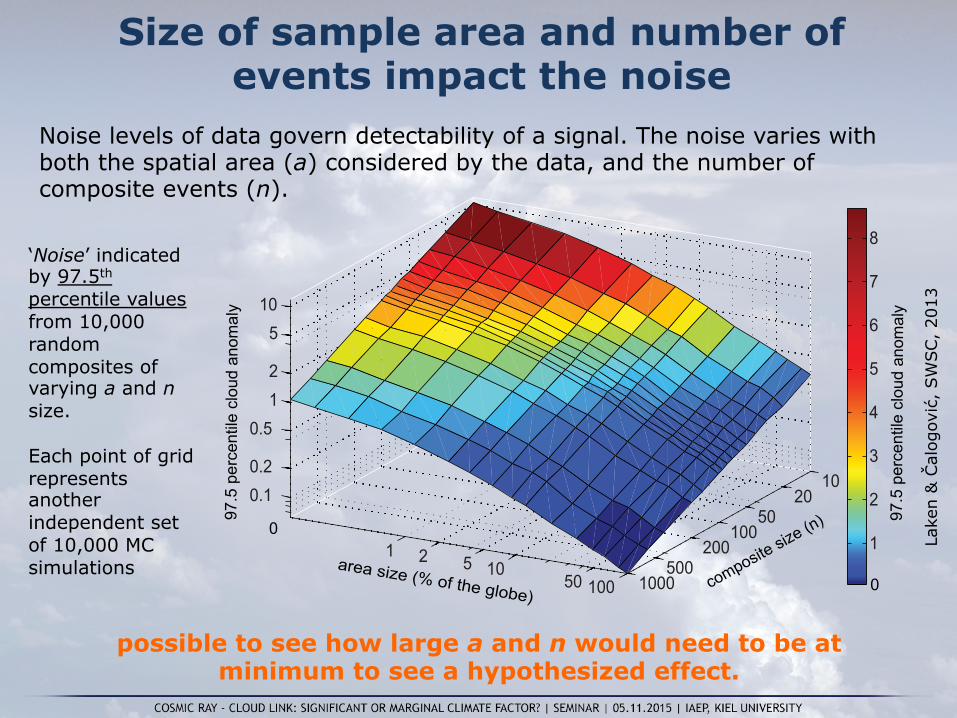
Noise levels of data govern detectability of a signal. The noise varies with both the spatial area (a) considered by the data, and the number of composite events (n).
1020
50100
200500
1000
1 2 5 1050 100
0.10.2
0.512
510
1
2
3
4
5
6
7
897
.5 p
erce
ntile
clo
ud a
nom
aly
composite size (n)0
area size (% of the globe)0
97.5
per
cent
ile c
loud
ano
mal
y
‘Noise’ indicated by 97.5th percentile values from 10,000 random composites of varying a and n size. Each point of grid represents another independent set of 10,000 MC simulations
possible to see how large a and n would need to be at minimum to see a hypothesized effect.
Size of sample area and number of events impact the noise
Lake
n &
Čal
ogov
ić,
SW
SC,
2013

Majority of Fd studies use less than 50 events (n<50)
Studies using only strong Fd events have usually less than 10 events
Size of Europe (2%)
• Satellite cloud es8mates are fraught with limita8ons and calibra8on errors, meaning long-‐term analysis is problema8c at best, and, as in the case of commonly used ISCCP data, is fundamentally flawed.
• Co-‐variance of solar-‐related parameters (UV, TSI, CR flux, solar wind) make signal awribu8on difficult.
• Climate variability and volcanic ac8vity, opera8ng over 8me-‐scales similar to the solar cycle, make disambigua8ng causes of cloud cover change difficult.
• Composite analysis of FD and GLE events is ooen compromised by the difficul8es of sta8s8cal analysis of autocorrelated data. This is compounded by the applica8on of inappropriate and black-‐box sta8s8cal tests.
• Changing signal-‐to-‐noise ra8os connected to spa8o-‐temporal restric8ons in composites have generally not been sufficiently taken into account in composite studies, leading to widespread type-‐1 (falseposi8ve) sta8s8cal errors.
There are numerous issues that may affect the results of solar-terrestrial studies
Some of these issues already discussed by Piwock (1978, 1979)

• Methodological differences and inappropriate sta8s8cs in composite analysis can produce conflic8ng results. These are the likely source of discrepancies between cosmic ray – cloud composite studies.
• Present cloud datasets are limited to detect a small changes in cloud cover as well to detect the regional cloud changes (<several thousand km) due to the big natural cloud variability (noise). Thus, localized and small effect on cloud cover can’t be completely excluded.
• No compelling evidence to support a cosmic ray cloud connec8on hypothesis using the satellite cloud data (ISCCP, MODIS) with long-‐ or short-‐term (Fd) studies.
• Cosmic rays doesn’t influence the global cloud cover and it is not a major factor in climate change or global warming! (opposite to believing of climate scep8cs)
Conclusions