INFLATION IN AUSTRALIA: CAUSES, INERTIA AND POLICY

Jerome Fahrer

Justin Myatt

Research Discussion Paper

9105

July 1991

Economic Research Department

Reserve Bank of Australia

We are grateful to colleagues at the RBA for helpful comments, especially Malcolm Edey. Any errors are ours alone. The views expressed herein are those of the authors and do not necessarily reflect the views of the R~serve Bank of Australia.

ABSTRACT

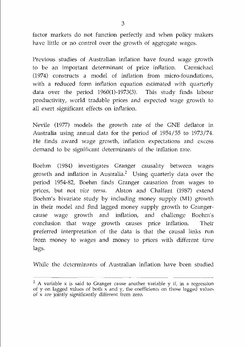
This paper examines the determination of inflation in Australia and its four major trading partners - Japan, the United States, the

United Kingdom and New Zealand. Also examined is the degree of inertia in the inflation rate i.e. the extent to which observed

inflation deviates from its equilibrium rate. We find that, in each

country, nominal wage growth clearly dominates the growth rate

of money as the fundamental cause of inflation. We also detect the presence of substantial inflation inertia. For Australia, these

findings have two implications for policy. The first is that a policy to reduce the inflation will have the desired effect only

after the elapse of a considerable period of time. The second is that such a policy can succeed only if aggregate nominal wage growth is reduced commensurately.

TABLE OF CONTENTS

1. Introduction

2. The Structural Model: Specification

(i) The Equilibrium Inflation Rate

(ii) Dynamics 10

3. Testing the Exogeneity of Nominal Wage Growth 12

4. Shor t-Run Determinants of Inflation

5. The Structural Model: Estimation

6. Policy Implications

References

Appendix 1: Granger Causality and Exogeneity 28

Appendix 2: Data Methods and Sources 29

Appendix 3: Tests for Serial Correlation and Heteroskedasticity

Appendix 4: Data 35

INFLATION IN AUSTRALIA: CAUSES, INERTIA AND POLICY

Jerome Fahrer and Justin Myatt

1. INTRODUCTION

Australia's inflation rate has been high since the early 1970's, both

in absolute terms and relative to the other developed market

economies.' Although the costs of this inflation have been difficult to quantify, most economists and policy makers agree that

decreasing the rate of inflation ought to be one of the leading priorities for macroeconomic policy.

In this paper, we aim to analyze Australia's inflation rate from

three perspectives. First, we examine the contributions of four factors - the growth rates of money, nominal wages and

productivity, and world inflation - to inflation in the short-term.

Second, we examine the contributions of these factors to the long- term (equilibrium) inflation rate. Third, we investigate how inuch inertia there is in the inflation rate, i.e. whether inflation can deviate from its equilibrium rate for a significant period of time.

For comparative purposes, we similarly examine inflation in

Australia's four major trading partners: Japan, the United States,

the United Kingdom and New Zealand.

Over the period 1973-1989 Australian and OECD average annual inflation rates (measured by the CPI) were 9.7 percent and 7.7 percent, respectively. In terms of GDP(GNP) deflators, they were 10.0 percent and 6.6 per cent respectively. (Sources: OECD Main Economic Indicators, Australian Bureau of Statistics Catalogue Nos. 6401.0 and 6442.0)

Carmichael (1990) provides an extensive overview of inflation in Australia during the 1980's.

We intend particularly to examine the importance of aggregate wage growth in the determination of price inflation. The control of wage inflation has always assumed a great deal of importai~ce in the making of Australian economic policy, often because of its perceived influence in restraining price inflation (Milbourne 1990). In recent years this argument has been used as one of the chief

justifications for the centralized wages system. Recently, however, the costs of this system viz. the reduced flexibility of relative wages, have received greater recognition and some steps have been taken towards a deregulated wages system. Such a system, however, necessarily implies that policy makers will lose some (perhaps all) direct control over aggregate wage outcomes.

This would not necessarily be an adverse development, of course,

provided goods and factor markets are competitive and clear continuously, i.e. prices in all markets are flexible. Under these circumstances, allocative efficiency suggests that the relative prices of various types of labour ought to be determined by relative scarcities, with the aggregate wage outcome of no more macroeconomic importance than, say, the aggregate peanut price outcome. Control of inflation can be achieved by control of an appropriate nominal quantity, such as the supply of money.

In practice, however, markets do not commonly reflect this competitive ideal. Wages are often determined by bargains between unions and firm. Relative wage outcomes, even when market determined, are often influenced by such irritating considerations as perceived fairness (Akerlof and Yellen 1990), while prices in imperfectly competitive markets will be determined as markups over costs (Blanchard and Fischer 1989, pp. 465-468). Under these circumstances, we have to ask whether a satisfactory

outcome for price inflation can be delivered when goods and

factor markets do not function perfectly and when policy makers have little or no control over the growth of aggregate wages.

Previous studies of Australian inflation have found wage growth to be an important determinant of price inflation. Carmichael

(1974) constructs a model of inflation from micro-foundations, with a reduced form inflation equation estimated with quarterly

data over the period 1960(1)-1973(3). This study finds labour productivity, world tradable prices and expected wage growth to

all exert significant effects on inflation.

Nevile (1977) models the growth rate of the GNE deflator in Australia using annual data for the period of 1954/55 to 1973/74.

He finds award wage growth, inflation expectations and excess demand to be significant determinants of the inflation rate.

Boehm (1984) investigates Granger causality between wages

growth and inflation in ~ u s t r a l i a . ~ Using quarterly data over the

period 1954-82, Boehm finds Granger causation from wages to

prices, but not vice versa. Alston and Chalfant (1987) extend Boehm's bivariate study by including money supply (MI) growth

in their model and find lagged money supply growth to Granger-

cause wage growth and inflation, and challenge Boehm's

conclusion that wage growth causes price inflation. Their

preferred interpretation of the data is that the causal links run

from money to wages and money to prices with different time

lags.

While the determinants of Australian inflation have been studied

A variable x is said to Granger cause another variable y if, in a regression of y on lagged values of both x and y, the coefficients on those lagged values of x are jointly significantly different from zero.

extensively, we are not aware of any previous work that has examined the degree of inertia in Australia's inflation rate. This stands in contrast to studies of inflation in other countries where the inertia issue has received some attention. Gordon (1985) finds lagged inflation to be a significant determinant of US inflation. In a recent study Gordon (1990) examines inflation in the US, UK, Japan, France and Germany over the period 1873-1987. He finds the emergence of considerable inertia in the last three decades for all countries except Japan.

The rest of the paper is organized as follows. In Section 2 we derive a structural model of the equilibrium inflation rate, and discuss dynamics which take into account possible inertia ill the adjustment of prevailing inflation to its equilibrium rate. In Section 3 we examine the exogeneity of money and nominal wages. Evidence pertaining to the short-term determinants of inflation is presented in Section 4. In Section 5 we report the results from the estimation of our dynamic model of the equilibrium inflation rate and draw some implications for policy in Section 6.

2. THE STRUCTURAL MODEL: SPECIFICATION

(i) The Equilibrium Inflation Rate

The equilibrium inflation rate is determined by the following three-equation structural model, with all the variables, except the nominal interest rate, i, specified as natural logarithms.

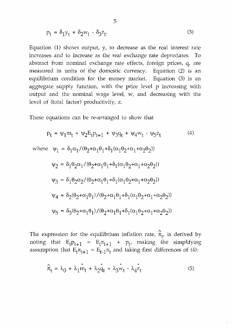
Equation (1) shows output, y, to decrease as the real interest rate

increases and to increase as the real exchange rate depreciates. To

abstract from nominal exchange rate effects, foreign prices, q, are measured in units of the domestic currency. Equation (2) is an

equilibrium condition for the money market. Equation (3) is an

aggregate supply function, with the price level p increasing with

output and the nominal wage level, w, and decreasing with the

level of (total factor) productivity, z.

These equations can be re-arranged to show that

where v1 = 6 1 a l / ( ~ 2 + ~ l ~ 1 + ~ 1 ( ~ 1 ~ 2 + ~ l + ~ 2 ~ 2 ) )

A The expression for the equilibrium inflation rate, 7tt, is derived by

noting that Etpt+l = Et7ttcl + pt, making the simplifying assumption that Etnt+l = E t-l 7t and taking first differences of (4):

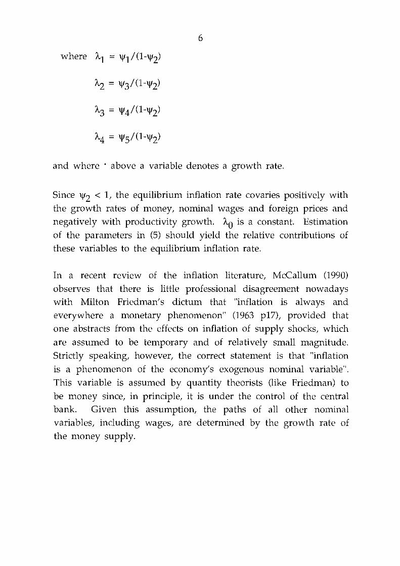
where hl = v1/(1-v2)

and where ' above a variable denotes a growth rate.

Since v2 < 1, the equilibrium inflation rate covaries positively with the growth rates of money, nominal wages and foreign prices and negatively with productivity growth. ho is a constant. Estimation of the parameters in (5) should yield the relative contributions of these variables to the equilibrium inflation rate.

In a recent review of the inflation literature, McCallum (1990) observes that there is little professional disagreement nowadays with Milton Friedman's dictum that "inflation is always and everywhere a monetary phenomenon" (1963 p17), provided that one abstracts from the effects on inflation of supply shocks, which are assumed to be temporary and of relatively small magnitude. Strictly speaking, however, the correct statement is that "inflation is a phenomenon of the economy's exogenous nominal variable". This variable is assumed by quantity theorists (like Friedman) to be money since, in principle, it is under the control of the central bank. Given this assumption, the paths of all other nominal variables, including wages, are determined by the growth rate of the money supply.

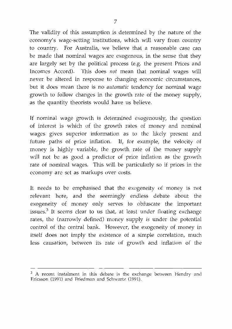
The validity of this assumption is determined by the nature of the economy's wage-setting institutions, which will vary from country to country. For Australia, we believe that a reasonable case can be made that nominal wages are exogenous, in the sense that they are largely set by the political process (e.g. the present Prices and Incomes Accord). This does not mean that nominal wages will never be altered in response to changing economic circumstances, but it does mean there is no automatic tendency for nominal wage growth to follow changes in the growth rate of the money supply, as the quantity theorists would have us believe.

If nominal wage growth is determined exogenously, the question of interest is which of the growth rates of money and nominal

wages gives superior information as to the likely present and future paths of price inflation. If, for example, the velocity of money is highly variable, the growth rate of the money supply will not be as good a predictor of price inflation as the growth rate of nominal wages. This will be particularly so if prices in the economy are set as markups over costs.

It needs to be emphasised that the exogeneity of money is not relevant here, and the seemingly endless debate about the exogeneity of money only serves to obfuscate the important issue^.^ It seems clear to us that, at least under floating exchange rates, the (narrowly defined) money supply is under the potential control of the central bank. However, the exogeneity of money in itself does not imply the existence of a simple correlation, i11uch less causation, between its rate of growth and inflation of the

A recent instalment in this debate is the exchange between Hendry and Ericsson (1991) and Friedman and Schwartz (1991).

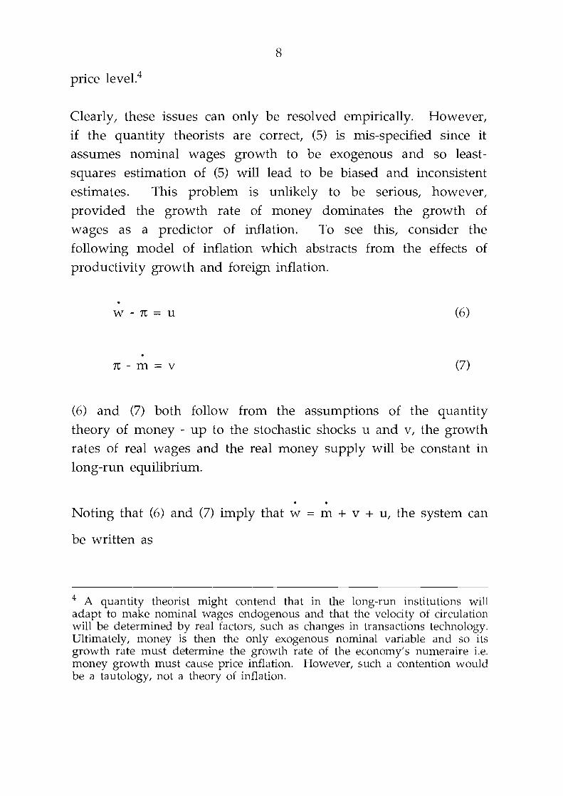
price leveL4

Clearly, these issues can only be resolved empirically. However,

if the quantity theorists are correct, (5) is mis-specified since it assumes nominal wages growth to be exogenous and so least-

squares estimation of (5) will lead to be biased and inconsistent estimates. This problem is unlikely to be serious, however,

provided the growth rate of money dominates the growth of wages as a predictor of inflation. To see this, consider the

following model of inflation which abstracts from the effects of

productivity growth and foreign inflation.

(6) and (7) both follow from the assumptions of the quantity

theory of money - up to the stochastic shocks LI and v, the growth rates of real wages and the real money supply will be constant in long-run equilibrium.

. . Noting that (6) and (7) imply that w = m + v + u, the system can

be written as

A quantity theorist might contend that in the long-run institutions will adapt to make nominal wages endogenous and that the velocity of circulation will be determined by real factors, such as changes in transactions technology. Ultimately, money is then the only exogenous nominal variable and so its growth rate must determine the growth rate of the economy's numeraire i.e. money growth must cause price inflation. However, such a contention would be a tautology, not a theory of inflation.

. = (<+z)m + <(u+v) + v where z = 1 and < = 0.

. A Since m is exogenous: the OLS estimate <+z is unbiased.

A However, < is biased since

The extent of the bias depends on the ratio o ,/o .. This ratio A

will be small and so will be close (but not equal) to zero provided money growth conveys significantly more information than nominal wage growth about inflation, which will certainly be . . the case when m is exogenous and w is endogenous.

. The case where both m and w are exogenous can be represented

by the model

where z is a stochastic error term.

No simultaneity bias arises here; the question of interest is the A

relative size of z and 0. This is easily resolved by noting that

Specifically, m is weakly exogenous i.e. inference for the model's parameters

can be made conditionally on m without loss of information. For an extensive discussion of the various types of exogeneity (weak, strong, strict and super), see Engle et al. (1983).

and

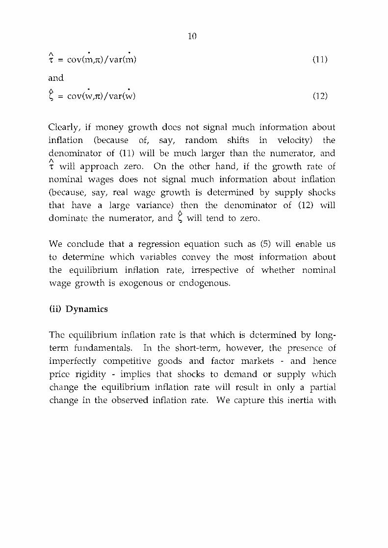
Clearly, if money growth does not signal much information about

inflation (because of, say, random shifts in velocity) the

denominator of (11) will be much larger than the numerator, and A z will approach zero. On the other hand, if the growth rate of

nominal wages does not signal much information about inflation

(because, say, real wage growth is determined by supply shocks that have a large variance) then the denominator of (12) will

dominate the numerator, and 2 will tend to zero.

We conclude that a regression equation such as (5) will enable us to determine which variables convey the most information about

the equilibrium inflation rate, irrespective of whether nominal

wage growth is exogenous or endogenous.

(ii) Dynamics

The equilibrium inflation rate is that which is determined by long-

term fundamentals. In the short-term, however, the presence of

imperfectly competitive goods and factor markets - and hence

price rigidity - implies that shocks to demand or supply which

change the equilibrium inflation rate will result in only a partial

change in the observed inflation rate. We capture this inertia with

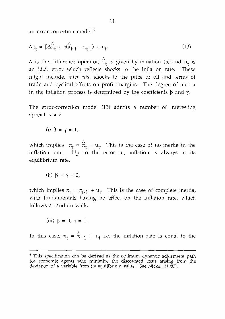
an error-correction model?

A A is the difference operator, nt is given by equation (5) and ut is

an i.i.d. error which reflects shocks to the inflation rate. These

might include, inter alia, shocks to the price of oil and terms of

trade and cyclical effects on profit margins. The degree of inertia

in the inflation process is determined by the coefficients P and y.

The error-correction model (13) admits a number of interesting

special cases:

(i) P = y = 1,

A which implies nt = xt + ut. This is the case of no inertia in the

inflation rate. Up to the error ut, inflation is always at its

equilibrium rate.

(ii) p = y = 0,

which implies nt = x ~ - ~ + ut. This is the case of complete inertia,

with fundamentals having no effect on the inflation rate, which

follows a random walk.

(iii) p = 0, y = 1.

A In this case, nt = nt-l + ut i.e. the inflation rate is equal to the

his specification can be derived as the optimum dynamic adjustment path for economic agents who minimize the discounted costs arising from the deviation of a variable from its equilibrium value. See Nickel1 (1985).

previous period's equilibrium rate.

(iv) p = 1, y = 0,

A which implies Axt = Axt + ut i.e. the change in the inflation rate

is equal to the change in the equilibrium rate, but the inflation

rate itself need not be at its equilibrium value.

3. TESTING THE EXOGENEITY OF NOMINAL WAGE GROWTH

In this section we test for the exogeneity of nominal wage growth. We do so by reporting, for each country, the variance

decompositions of wage and money growth obtained from a

vector autoregression (VAR) estimated over the period 1964-1989.~

Consider the autoregressive process y, = b(L)y, + u,. y is an nxl

vector of stationary variables, u is an nxl vector of innovations

(forecast errors) and b(L) is an nxT matrix of autoregressive parameters, where L is the lag operator and T is the lag length of the autoregression. Wold's representation theorem states this process can be expressed as the vector moving average y, = a(L)u,

+ E(u,) where the coefficients of the matrix a(L) are functions of

the estimated autoregressive parameters b(L). a(L) at lag 0 is the

identity matrix. Each variable is therefore expressed as the sum of

current and past innovations of all the variables in the system.

The variance decomposition assigns the total variance of the k-step ahead forecast error to innovations in the variables of the system, via the MA representition.

Because of data limitations, the estimation period for New Zealand starts in 1965.

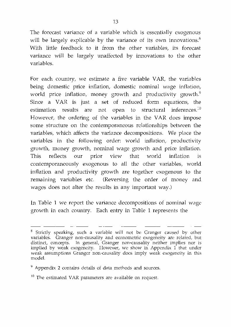
The forecast variance of a variable which is essentially exogenous

will be largely explicable by the variance of its own innovations.'

With little feedback to it from the other variables, its forecast

variance will be largely unaffected by innovations to the other variables.

For each country, we estimate a five variable VAR, the variables being domestic price inflation, domestic nominal wage inflation, world price inflation, money growth and productivity

Since a VAR is just a set of reduced form equations, the

estimation results are not open to structural inferences."

However, the ordering of the variables in the VAR does impose some structure on the contemporaneous relationships between the variables, which affects the variance decompositions. We place the variables in the following order: world inflation, productivity

growth, money growth, nominal wage growth and price inflation. This reflects our prior view that world inflation is

contemporaneously exogenous to all the other variables, world

inflation and productivity growth are together exogenous to the

remaining variables etc. (Reversing the order of money and wages does not alter the results in any important way.)

In Table 1 we report the variance decompositions of nominal wage growth in each country. Each entry in Table 1 represents the

Strictly speaking, such a variable will not be Granger caused by other variables. Granger non-causality and econometric exogeneity are related, but distinct, concepts. In general, Granger non-causality neither implies nor is implied by weak exogeneity. However, we show in Appendix 1 that under weak assumptions Granger non-causality does imply weak exogeneity in this model.

Appendix 2 contains details of data methods and sources.

lo The estimated VAR parameters are available on request.

Table 1

Variance Decomposition of Nominal Wage Growth

Percentage of Nominal Wage Growth Explained by Shock to:

World Productivity Money Nominal Wage Inflation Inflation Growth Growth Growth

Australia

Year

Japan

Year 1 15.9

2 13.3

3 28.9

4 27.5

5 25.2

New Zealand

Year 1 12.2 2 8.2

3 10.0

4 11.1

5 11.2

Table 1 (cont.)

Variance Decomposition of Wages Growth

Percentage of Nominal Wage Growth Explained by Shock to:

World Productivity Money Nominal Wage Inflation Inflation Growth Growth Growth

United Kingdom

Year

1 11.5 2 7.5

3 10.5 4 13.2

5 15.2

United States

Year 1 0.2

2 7.8

3 11.7 4 15.8

proportion of nominal wage growth, at each time lag, associated

with shocks to each variable in the model. By construction, these shocks are uncorrelated, so the proportions sum to 100 per cent. We use two lags of each variable in each VAR.

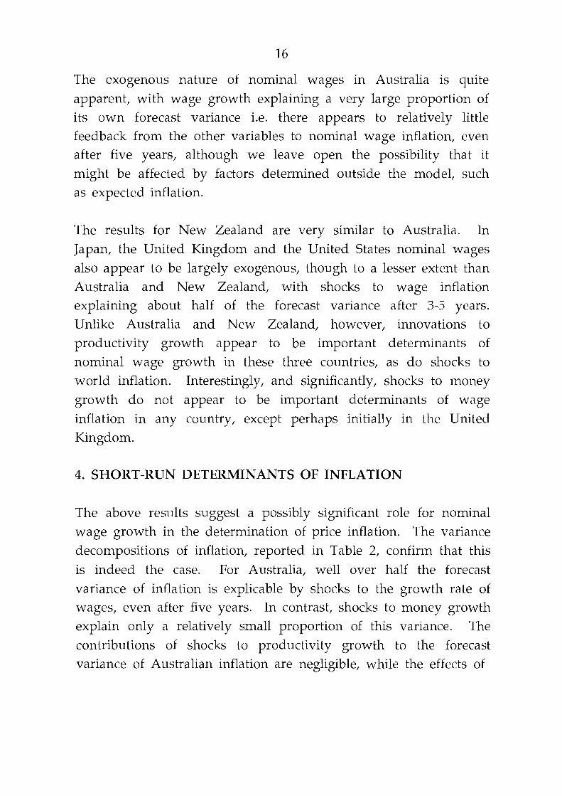
The exogenous nature of nominal wages in Australia is quite

apparent, with wage growth explaining a very large proportion of its own forecast variance i.e. there appears to relatively little feedback from the other variables to nominal wage inflation, even after five years, although we leave open the possibility that it

might be affected by factors determined outside the model, such

as expected inflation.

The results for New Zealand are very similar to Australia. In

Japan, the United Kingdom and the United States nominal wages

also appear to be largely exogenous, though to a lesser extent than Australia and New Zealand, with shocks to wage inflation explaining about half of the forecast variance after 3-5 years.

Unlike Australia and New Zealand, however, innovations to

productivity growth appear to be important determinants of nominal wage growth in these three countries, as do shocks to

world inflation. Interestingly, and significantly, shocks to inoney

growth do not appear to be important determinants of wage

inflation in any country, except perhaps initially in the United

Kingdom.

4. SHORT-RUN DETERMINANTS OF INFLATION

The above results suggest a possibly significant role for nominal

wage growth in the determination of price inflation. The variance

decompositions of inflation, reported in Table 2, confirin that this

is indeed the case. For Australia, well over half the forecast

variance of inflation is explicable by shocks to the growth rate of wages, even after five years. In contrast, shocks to money growth

explain only a relatively small proportion of this variance. The contributions of shocks to productivity growth to the forecast

variance of Australian inflation are negligible, while the effects of

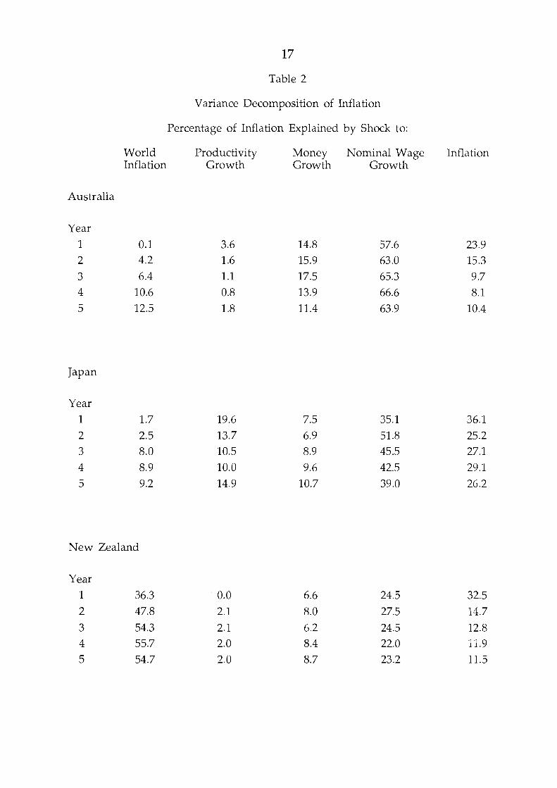
Table 2

Variance Decomposition of Inflation

Percentage of Inflation Explained by Shock to:

World Productivity Money Nominal Wage Inflation Inflation Growth Growth Growth

Australia

Year 1 0.1

2 4.2

3 6.4 4 10.6

5 12.5

Japan

Year 1 1.7

2 2.5

3 8.0 4 8.9

5 9.2

New Zealand

Year 1 36.3

2 47.8

3 54.3 4 55.7

5 54.7

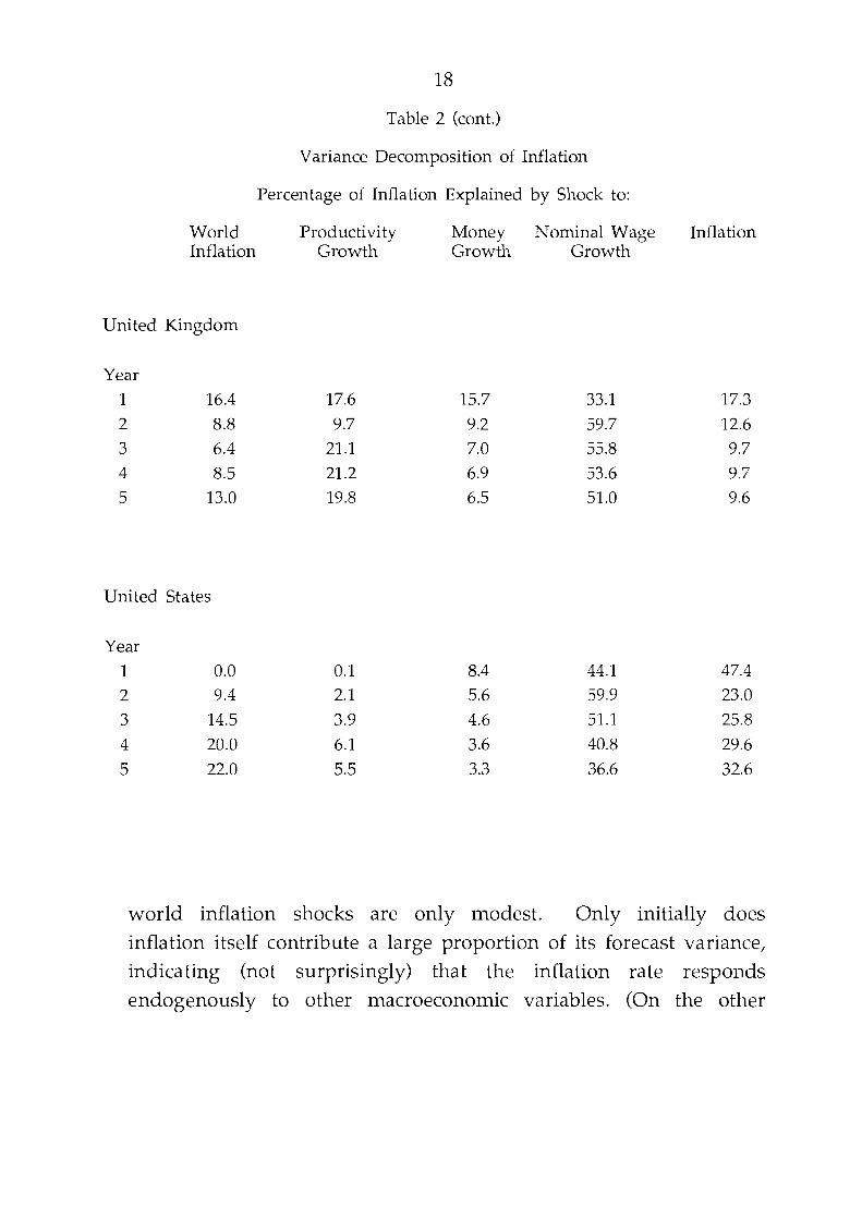
Table 2 (cont.)

Variance Decomposition of Inflation

Percentage of Inflation Explained by Shock to:

World Productivity Money Nominal Wage Inflation Inflation Growth Growth Growth

United Kingdom

Year 1 16.4 17.6

2 8.8 9.7

3 6.4 21.1

4 8.5 21.2

5 13.0 19.8

United States

Year 1 0.0 0.1 2 9.4 2.1

3 14.5 3.9 4 20.0 6.1

5 22.0 5.5

world inflation shocks are only modest. Only initially does inflation itself contribute a large proportion of its forecast variance, indicating (not surprisingly) that the inflation rate responds

endogenously to other macroeconomic variables. (On the other

hand, Fahrer and Shori (1990) find that inflationary expectations in Australia appear to be largely exogenous.)

The variance decompositions for the other four countries indicate that wages co~~sistently dominate money as explanators of inflation. Soine interesting cross-country differences do however arise. New Zealand stands out in that world inflation appears to be a important determinant of its domestic inflation, where it accounts for about 50 per cent of the forecast variance after two years. Productivity growth plays a significant role in Japan and the United Kingdom, but not elsewhere.

5. THE STRUCTURAL MODEL: ESTIMATION

The variance decompositions pertain to the deteri~~ination of inflation in the short-run. In this section we examine the determinants of the long-run, equilibrium, inflation rate.

The estimating equation for the stn~ctural model of Section 2 is derived by substituting equation (5) into equation (13):

Equation (14) is non-linear in the parameters P, y, Lo, hl, h2, % and h4. There are five such equations in our model, corresponding to each of the five countries that we examine. We think it is reasonable to presume that contemporaneous inflation disturbances could be correlated across countries and so we estimate the model by i~on-linear Seemingly Unrelated Regressions.

Table 3 Parameter Estimates

(standard errors in parentheses)

Australia Japan New United United Zealand Kingdom States

SC(*) and HS(') are Breusch-Pagan test statistics for serial corr lation and heteroskedasticity, respectively. All are distributed as 2 (1 ) . See Appendix 3 for details.

The model is estimated using annual data over the period 1964-89.

The estimation results are reported in Table 3. They are very encouragng. The fit of all the equations is good; there is no evidence of any serial correlation in the residuals and only for Australia is there any evidence of heteroskeda~ticit~." In general, the estimated standard errors are small relative to the coefficient estimates. Very few of the estimated parameters have the wrong sign and, of the ones that do, none is significantly different from zero at the one percent level.

The estimates of y show that in Japan only about 30 percent of the disequilibrium inflation is reflected in the change in inflation

the following year, compared with about 50 per cent in Australia, 60 percent in the United Kingdom, 80 per cent in the United States and 90 per cent in New Zealand. The estimates of P, which indicate the proportion of the change in the equilibrium inflation rate that is observed contemporaneously, also vary markedly across countries. Here the relative rankings of Japan and New Zealand are reversed, with the greatest change occurring in Japan

(about 80 percent) and the least change in New Zealand (about 50 percent). Australia has the median estimate with 63 percent.

Generally speaking, the overall degree of inflation inertia (given by the sum of P and y) does not vary greatly across countries. However, the divergence of the estimated p's and y s indicates

that the nature of the inflation dynamics does vary across countries. Australian inflation displays slightly more inertia than

- - -

" Specifically, at the five per cent level of significance, we can reject the null hypothesis that the variance of inflation errors in Australia is unrelated to predicted inflation. However, since we are conducting 25 tests, we would expect at this level of significance to spuriously reject one null hypothesis.

the international average, but this difference is not terribly large.

The estimated values of the equilibrium inflation parameters (the

h's) show a consistent pattern across the five countries. In particular, in every country, nominal wage growth appears to be far more important than the growth of money in determining the steady state inflation rate (h3 > hl). In the Australian case, for example, a five percent increase in wage growth leads to an increase in the equilibrium inflation rate of about four per cent, while the same increase in money growth leads to an increase in equilibrium inflation of slightly more than one percent.

A determined quantity theorist would no doubt interpret these results differently, arguing that nominal wages are not exogenous and the apparent causation from wages to prices masks the true structural relationship, which runs from money to wages and prices. While we do not deny the likelihood that tighter monetary policy will exert some downward pressure on wages growth, either through expectations of lower price inflation or through a weaker labour market, we nevertheless believe that such an argument would be beside the point.

Our interpretation of these results is that whatever the source of any disinflationary impulse, the response of wages is of paramount importance if inflation is to be reduced on a sustained basis. In a world where labour markets resemble the textbook

model of perfect competition, a tightening of monetary policy will almost certainly be accompanied by a rapid fall in nominal wage growth, and concomitantly, price inflation. In the real world

where the nature and behaviour of labour market institutions

matters, such a response is not guaranteed. A tightening of monetary policy that is not accompanied by a slowing of wage

growth will lead to a fall in inflation, but only via a contractioi~ of profit margins. This strategy might be effective in the short-run but is unlikely to prove an acceptable method of lowering the inflation rate over a long time horizon.

The estimates of h4 show that increased productivity growth reduces inflation, as we would expect, but the extent of this reduction varies markedly across countries. The size of the coefficients shows, moreover, that the quantitative effect on inflation of increased productivity growth is likely to be modest. For example, suppose that "microeconomic reform" permanently increases the rate of total factor productivity growth in Australia by two percentage points per year, which would seem to us to be the upper bound for what might be achieved. The resultant fall in the steady state inflation rate will only be about one percent.

The estimates of + show that foreign inflation (measured in domestic currency), in every country except New Zealand, has negligible effects on the equilibrium inflation rate. This means that, New Zealand aside, foreign inflation has no explanatory power beyond that of the other variables.

6. POLICY IMPLICATIONS

We see two policy implications from the results of this paper. The first is that the inertia in Australia's inflation rate implies that policy action which seeks a reduction in inflation will produce the desired result only after a substantial period of time. The second is that nominal wage growth is the principal determinant of price

inflation in Australia. This poses a dilemma for policy makers. The deregulation of the labour market, with wages determined

(perhaps) on an enterprise by enterprise basis, should facilitate

efficiency-enhancing movements in relative wage levels. However, wages policy, as such, will then cease to exist as an instrument for combating inflation.

We could appeal to the Lucas critique (Lucas 1976) and assert that such a major policy change will fundamentally alter the structure

of the economy, rendering obsolete both our estimated relationships and the need for a wages policy. However, this remains very much to be seen. In any case, the demise of wages policy implies that the entire burden of keeping the rate of price inflation acceptably low will fall to monetary policy, whose role shall then be to deliver the correct anti-inflation signals to price and wage setters. This will be a difficult assignment in an economy where goods and factor markets work only imperfectly, where wage levels are set as the result of bargaining outcomes, and where prices are set as markups over costs.

REFERENCES

Akerlof, George and Janet A. Yellen (1990), "The Fair Wage-effort Hypothesis and Unemployment", Quarterly Journal of Econonzics, 105(2), 255-283, May.

Alston, Julian M. and James A. Chalfant (1987), "A Note 011 the Causality Between Money, Wages and Prices in Australia", Economic Record, 63, No. 181, 115-1 19, June.

Blanchard, Olivier Jean and Stanley Fischer (1989), Lectures on Macroeconomics, Cambridge MA: MIT Press.

Boehm, E.A. (1984), "Money Wages, Consumer Prices, and Causality in Australia", Economic Record, 60(170), 236-251, September.

Carmichael, Jeffrey (1974), "Modelling Inflation in Australia", Seminar Paper No. 39, Monash University, Melbourne.

Carmichael, Jeffrey (1990), "Inflation: Performance and Policy", in Stephen Grenville (ed.), The Australian Macroeconomy in the 1980s, Sydney: Reserve Bank of Australia.

Engle, Robert E., David F. Hendry and Jean-Francois Richard (1983), "Exogeneity", Econornetrica, 51(2), 277-304, March.

Fahrer, Jerome and Lynne-Ellen Shori (1990), "An Empirical Model of Australian Interest Rates, Exchange Rates and Monetary Policy", Reserve Bank of Australia Discussion Paper 9009.

Friedman, Milton (1963), Inflation: Causes and Consequences, New York: Asia Publishing House.

Friedman, Milton and Anna J. Schwartz (1991), "Alternative Approaches to Analyzing Economic Data", American Economic Review, 81(1), 39-49, March.

Gordon, Robert J. (1985), "Understanding Inflation in the 1980sU, Brookings Papers on Economic Activity, 1, 263-302.

Gordon, Robert J. (1990), "What is New-Keynesian Economics?",

Journal of Economic Literature, XXVIII, 1151-1171, September.

Hendry, David F. and Neil R. Ericsson (1991), "An Econometric Analysis of U.K. Money Demand in Monetary Trends in the United States and the United Kingdom by Milton Friedman and Anna J. Schwartz", American Economic Review, 81(1), 8-38, March.

Lucas, Robert E Jr. (1976) ,"Econometric Policy Evaluation: A Critique", in Karl Brunner and Alan H. Meltzer (eds.), The Phillips Curve and Labor Markets, Carnegie-Rochester Series on Public Policy.

McCallum, Bennett T. (1990), "Inflation: Theory and Evidence", in Benjamin M. Friedman and Frank H. Hahn (eds.), Handbook of Monetary Ecolzomics, Volume 2, Amsterdam: Elsevier Science

Publishers B.V.

Milbourne, Ross (1990), "Money and Finance", in Stephen Grenville (ed.), The Australian Macroeconomy in the 1980s, Sydney:

Reserve Bank of Australia.

Nevile, J.W. (1977), "Domestic and Overseas Influences on Inflation in Australia", Australian Economic Papers, 16(28), 121-129, June.

Nickell, Stephen (1985), "Error Correction, Partial Adjustment and all that: An Expository Note", Oxford Bulletin of Economics and Statistics, 47(2), 119-129, May.

Stewart, Brian P. (1986), "A Strategy for the Development of Individual Equations in Medium and Large Scale Macroeconometric Models", Economic Planning Advisory Council Technical Paper, No. 1, Office of the Economic Planning Advisory Council, March.

Appendix 1: Granger Causality and Exogeneity

In this appendix we demonstrate that, under weak assumptions, Granger non-causality implies weak exogeneity. Consider the following structural model of inflation:

. where a is the rate of inflation, m is the growth rate of money . and w is the growth rate of nominal wages. m is weakly . exogenous (with respect to the variables a and w). w is weakly . exogenous if b2 = b3 = 0. Conditional on this being true, w is an . exogenous determinant of a if a3 # 0, while m is an exogenous

determinant of a if a2 # 0.

The reduced form of this system is:

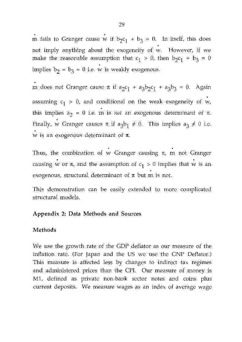
m fails to Granger cause w if b2cl + b3 = 0. In itself, this does

not imply anything about the exogeneity of w. However, if we make the reasonable assumption that cl > 0, then b2cl + b3 = 0

implies b2 = b3 = 0 i.e. w is weakly exogenous.

m does not Granger cause x if a2cl + a3b2cl + a3b3 = 0. Again

assuming cl > 0, and conditional on the weak exogeneity of w,

this implies a2 = 0 i.e. m is not an exogenous determinant of n.

Finally, w Granger causes n if a3bl # 0. This implies a3 # 0 i.e.

w is an exogenous determinant of x.

Thus, the combination of w Granger causing n, m not Granger

causing w or x, and the assumption of cl > 0 implies that w is an

exogenous, structural determinant of x but m is not.

This demonstration can be easily extended to more complicated structural models.

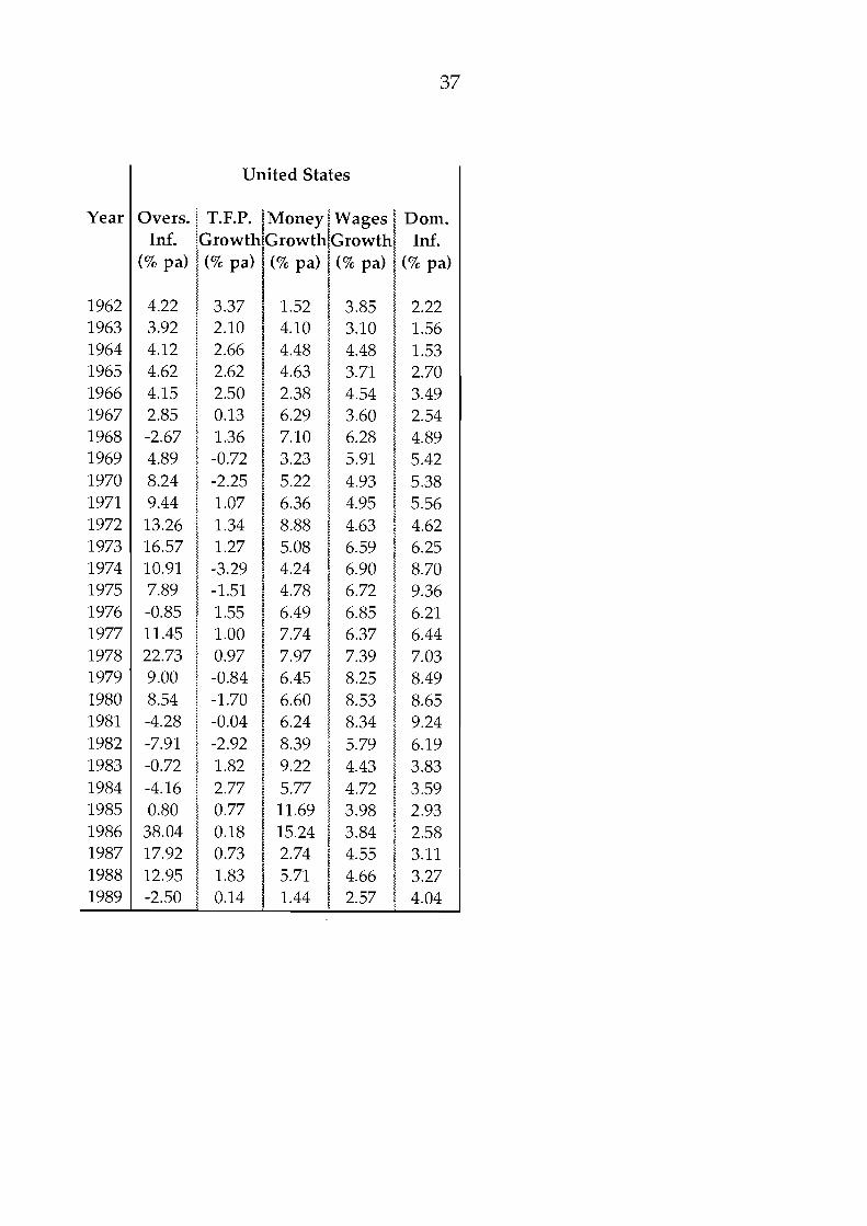
Appendix 2: Data Methods and Sources

Methods

We use the growth rate of the GDP deflator as our measure of the inflation rate. (For Japan and the US we use the GNP Deflator.) This measure is affected less by changes to indirect tax regimes

and administered prices than the CPI. Our measure of money is MI, defined as private non-bank sector notes and coins plus

current deposits. We measure wages as an index of average wage

rates.

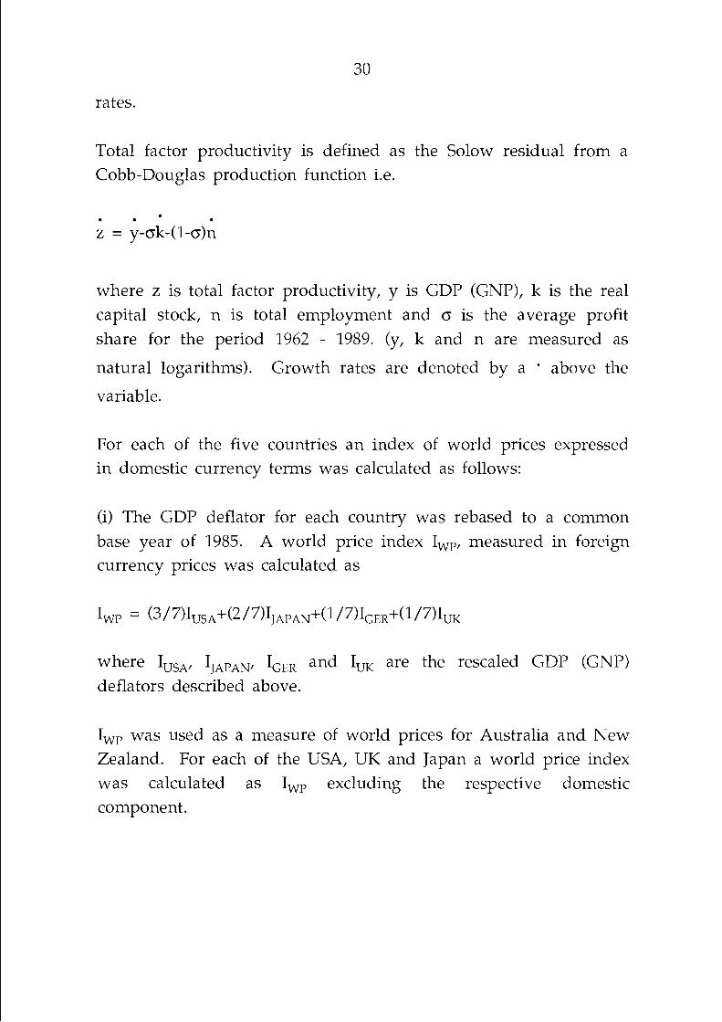
Total factor productivity is defined as the Solow residual from a Cobb-Douglas production function i.e.

where z is total factor productivity, y is GDP (GNP), k is the real capital stock, n is total employment and 0 is the average profit share for the period 1962 - 1989. (y, k and n are measured as

natural logarithms). Growth rates are denoted by a ' above the

variable.

For each of the five countries an index of world prices expressed in domestic currency terms was calculated as follows:

(i) The GDP deflator for each country was rebased to a common base year of 1985. A world price index I,,,, measured in foreign currency prices was calculated as

where IUSA, IJAPAN, IGER and IuK are the rescaled GDP (GNP) deflators described above.

I,, was used as a measure of world prices for Australia and New Zealand. For each of the USA, UK and Japan a world price index was calculated as I,, excluding the respective domestic component.

(ii) Exchange rates for five currencies against the USD (the Japanese yen (JPY), the Australian dollar (AUD), the New Zealand dollar (NZD), the Deutsche Mark(DEM) and the Pound Sterling (GBP)) were rescaled to a common base year of 1985.

An index of the domestic price of foreign currency (FC) was compiled for each of the five countries under study. For Australia, the index was computed as

The NZD index was computed with the same weights against the same four major currencies. For the USD price of foreign currency, the index consisted of JPY, DEM and GBP components and similarly for the JPY, DEM and GBP indexes.

(iii) For each country, an index of world prices measured in domestic currency terms was computed by multiplying the current world price index by the appropriate exchange rate index. For instance, for Australia, this index is given by:

Log differences of Q were then used as a measure of world inflation in domestic currency.

Sources

Real GDP (Y): All real GDP series taken from "Gross

National/Domes~ic Product: Volume", in OECD Economic Outlook.

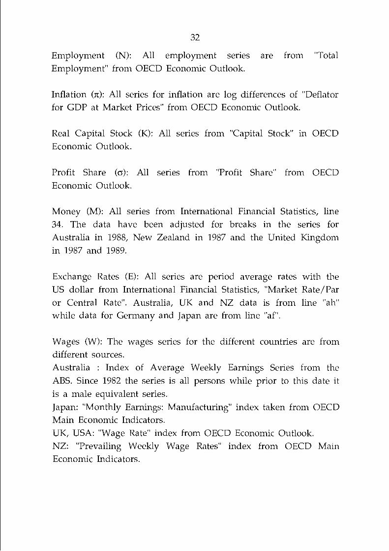
Employment (N): All employment series are from "Total Employment" from OECD Economic Outlook.

Inflation (d: All series for inflation are log differences of "Deflator for GDP at Market Prices" from OECD Economic Outlook.

Real Capital Stock (K): All series from "Capital Stock" in OECD Economic Outlook.

Profit Share (o): All series from "Profit Share" from OECD Economic Outlook.

Money (M): All series from International Financial Statistics, line 34. The data have been adjusted for breaks in the series for Australia in 1988, New Zealand in 1987 and the United Kingdom

in 1987 and 1989.

Exchange Rates (E): All series are period average rates with the US dollar from International Financial Statistics, "Market Rate/Par or Central Rate". Australia, UK and NZ data is from line "ah" while data for Germany and Japan are from line "af".

Wages (W): The wages series for the different countries are from different sources. Australia : Index of Average Weekly Earnings Series from the ABS. Since 1982 the series is all persons while prior to this date it

is a male equivalent series. Japan: "Monthly Earnings: Manufacturing" index taken from OECD Main Economic Indicators. LTK, USA: "Wage Rate" index from OECD Economic Outlook. NZ: "Prevailing Weekly Wage Rates" index from OECD Main Economic Indicators.

Appendix 3: Tests for Serial Correlation and Heteroskedasticity

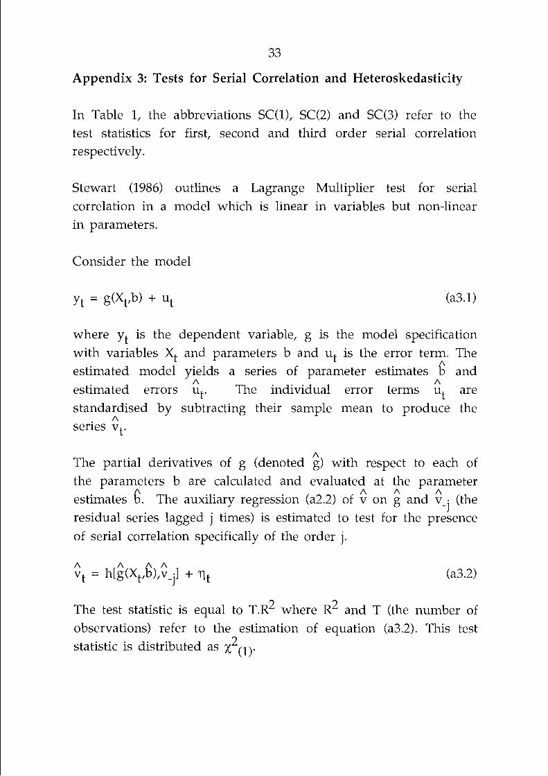
In Table 1, the abbreviations SC(l), SC(2) and SC(3) refer to the test statistics for first, second and third order serial correlation respectively.

Stewart (1986) outlines a Lagrange Multiplier test for serial correlation in a model which is linear in variables but non-linear in parameters.

Consider the model

where yt is the dependent variable, g is the model specification with variables Xt and parameters b and ut is the error term. The estimated model vields a series of parameter estimates 6 and

J I A A

estimated errors ut. The individual error terms ut are standardised by subtracting their sample mean to produce the

A series vt.

A The partial derivatives of g (denoted g) with respect to each of the parameters b are calculated and evaluated at the parameter

A A A A estimates b. The auxiliary regression (a2.2) of v on g and v (the -1 residual series lagged j times) is estimated to test for the presence of serial correlation specifically of the order j.

The test statistic is equal to T . R ~ where R2 and T (the number of observations) refer to the estimation of equation (a3.2). This test

2 statistic is distributed as x

34

The abbreviations HS(1) and HS(2) in table 1 denote tests for different forms of heteroskedasticity of the residuals.

Stewart outlines how the Breusch-Pagan test can be used to test for heteroskedasticity related to a time trend (HS(1)) or the value of predicted dependent variable (HS(2)).

A Using the error term series vt outlined above, equation (a3.3) is estimated:

A where G2 is the sample variance of vt, Zt is the variable

potentially related to the heteroskedasticity of vt, KO and rl are parameters and ut is an error term. For HS(l), Zt is a time trend. For HS(2), Zt is the predicted value of dependent variable in the primary estimation (from equation a3.1).

In both cases, the test statistic is equal to T . R ~ where R2 and T (the number of observations) refer to the estimation of equation

2 (a3.3). This test statistic is distributed as x

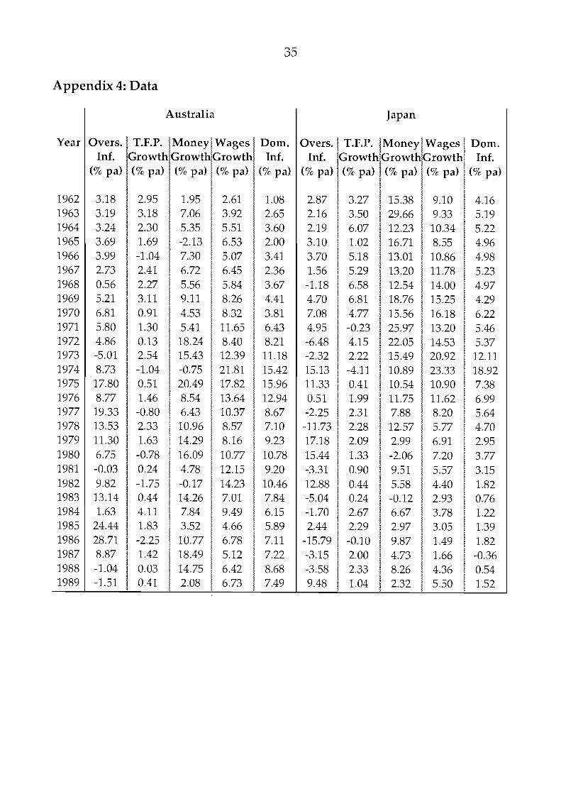
Appendix 4: Data

Year

1962 1963 1964 1965 1966 1967 1968 1969 1970 1971 1972 1973 1974 1975 1976 1977 1978 1979 1980 1981 1982 1983 1984 1985 1986 1987 1988 1989

Australia

Overs. Inf.

(% pa)

3.18 3.19 3.24 3.69 3.99 2.73 0.56 5.21 6.81 5.80 4.86 -5.01 8.73 17.80 8.77 19.33 13.53 11.30 6.75 -0.03 9.82 13.14 1.63

24.44 28.71 8.87 -1.04 -1.51

T.F.P. Growth (% pa)

Dom. Inf.

(% pa)

1.08 2.65 3.60 2.00 3.41 2.36 3.67 4.41 3.81 6.43 8.21 11.18 15.42 15.96 12.94 8.67 7.10 9.23 10.78 9.20 10.46 7.84 6.15 5.89 7.11 7.22 8.68 7.49

Overs. Inf.

(% pa)

2.87 2.16 2.19 3.10 3.70 1.56 -1.18 4.70 7.08 4.95 -6.48 -2.32 15.13 11.33 0.51 -2.25 -11.73 17.18 15.44 -3.31 12.88 -5.04 -1.70 2.44

-15.79 -3.15 -3.58 9.48

T.F.P. IGr owt l / (% pa)

3.27 I

I 2; I 1.02 1 5.18 1 5.29 1 6.58 I 6.81 1 4.77 1 -0.23 1 4.15 1 2.22 1 -4.11

0.41 1 1.99 1 2.31

j ;::; 1.33 0.90

/ 0.44 1 0.24 1 2.67 1 2.29 i -0.10 I 2.00 1 2.33 1 1.04

/Money/ Wages ~$GrowtqGrowth

1 (% pa) / (% pa)

Dom. Inf.

(% pa)

4.16 5.19 5.22 4.96 4.98 5.23 4.97 4.29 6.22 5.46 5.37 12.11 18.92 7.38 6.99 5.64 4.70 2.95 3.77 3.15 1.82 0.76 1.22 1.39 1.82 -0.36 0.54 1.52

Year

1962 1963 1964 1965 1966 1967 1968 1969 1970 1971 1972 1973 1974 1975 1976 1977 1978 1979 1980 1981 1982 1983 1984 1985 1986 1987 1988 1989

Overs. Inf.

(% pa)

3.13 3.22 3.30 3.63 4.17 4.80 19.9 5.33 6.63 5.84 5.10 -0.57 7.19

22.60 21.97 11.96 10.01 10.39 13.56 12.14 12.21 12.86 13.60 16.61 19.36 0.99 -0.04 8.72

New Zealand

T.F.P. Growth (% pa)

Dom. Inf.

(% pa)

6.05 3.92 3.77 4.11 0.71 3.47 5.53 3.17 6.84 12.25 9.20 10.00 3.08 9.71 17.08 16.84 13.09 16.19 13.76 15.67 12.11 6.00 7.09 12.12 14.98 14.18 8.26 5.74

Overs. Inf.

(% pa)

3.16 3.30 3.28 3.55 3.94 4.98 18.16 5.35 6.94 5.48 7.91 16.66 15.39 13.65 26.29 13.57 6.89 -3.67 -3.95 15.96 13.69 17.68 13.1 4.63

-21.31 -4.29 -7.05 0.11

United Kingdom

T.F.P. Growth (% pa)

~ o n e ~ i Wages 1 Dom.

5 i Growt :Growth! Inf.

! I (% pa) 1 (% pa) (% pa)

2 i

* denotes missing value

Year Overs. Inf.

(% pa)

United States

T.F.P. Growtl (% pa)

I Wages f Dom. I

~,Growthl Inf. 1 (% pa) r (% pa) I