Sacrifice Ratio and Cost of Inflation for the Indian Economy · Sacrifice Ratio and Cost of...

Sacrifice Ratio and Cost of Inflation for the Indian Economy

Ravindra H. Dholakia

W.P. No. 2014-02-04 February 2014

The main objective of the working paper series of the IIMA is to help faculty members, research staff and

doctoral students to speedily share their research findings with professional colleagues and to test out their research findings at the pre-publication stage.

INDIAN INSTITUTE OF MANAGEMENT AHMEDABAD-380 015

INDIA

IIMA �INDIA Research and Publications

Page No. 2 W.P. No. 2014-02-04

Sacrifice Ratio and Cost of Inflation for the Indian Economy

Ravindra H. Dholakia

IIM Ahmedabad1

E-mail : [email protected]

ABSTRACT

Traditional concept of the Sacrifice Ratio measures the loss of potential output sustained by the

society in the medium term to achieve reduction in the long-run inflation by one percentage

point. This concept is critically examined and generalized to include episodes increasing the

long-run inflation rate to gain higher growth of output and employment and hence reduction in

the poverty proportion in the medium term. Since the concept needs measurement through a

shifting short-run equilibrium of dynamic aggregate demand and supply in terms of inflation rate

and output attributable to monetary policy interventions, its estimation is challenging. There are

two alternative approaches to estimate the ratio, the direct one and regression based. Both have

their relative merits and demerits. The regression based approach provides one unique average

estimate of the Sacrifice Ratio for all episodes but allows holding other factors constant. The

direct approach provides separate estimates by episodes but fails to hold other factors constant.

The Sacrifice Ratio turns out to be in a narrow range of 1.8 to 2.1 for deliberate deflation and

2.8 for inflation in India. On the other hand, benefits of one percentage point reduction in trend

rate of inflation are at best 0.5 percentage points increase in long-term growth of output that

occurs after 4-5 years. This has implications on policy to disinflate.

I. Introduction

Sacrifice Ratio essentially represents the cost of permanently reducing inflation in terms

of possible loss of output. It is, therefore, a very relevant concept for the policy makers, but its

empirical estimation involves practical difficulties that make it less reliable for direct application.

As such, there are only two serious efforts to estimate the Sacrifice Ratio for the Indian economy

(RBI, 2002; and Kapur & Patra, 2003). RBI (2002) reports only one estimate of +2 for the

1 Data collection and computational assistance provided by Mr. Shrikant Taparia is gratefully acknowledged.


Page No. 3 W.P. No. 2014-02-04

Sacrifice Ratio for India. On the other hand, Kapur & Patra (2003) have shown that the estimates

of the Sacrifice Ratio for the Indian economy differ widely depending on: (a) measure of

inflation- whether WPI based or GDP deflator based; (b) time period considered; and (c)

alternative specifications of the short-run aggregate supply equation. Their estimates vary from

0.3 to 4.7 and in some of the cases the estimates were not statistically significantly different from

zero. Such a wide range of estimates of the ratio is also a feature of the empirical studies for

various other countries like USA, Canada, Australia, New Zealand and OECD countries (see

Kapur & Patra, 2003 for summary with references).

Thus, there is a need to examine the precise concept of the Sacrifice Ratio and methods to

estimate it, particularly for a fast growing economy like India. The present paper discusses the

concept of the Sacrifice Ratio within the standard macroeconomic theory and considers some of

its features not emphasized in the literature in the next section. The third section critically

reviews various methods to estimate it. It also presents the estimates of the ratio for the Indian

Economy by appropriate methods in the fourth section. The fifth section discusses the cost of

inflating or the benefits of disinflating in the long-run in the Indian context and the last section

provides concluding remarks with some policy implications.

II. Concept of the Sacrifice Ratio

Standard textbooks define the Sacrifice Ratio as percentage of a year’s real output lost in

order to obtain 1 percentage point reduction in the inflation rate (see Mankiw, 2010, p.396 and

Dornbusch, Fischer & Startz, 2012, p.147). Whatever empirical evidence exists on various

economies suggests that efforts to reduce inflation on permanent basis invariably involve some

cost in terms of the temporarily increased unemployment and lower output over medium term.

The literature considers the Sacrifice Ratio only when there is a deliberate effort by the

monetary authority to reduce the inflation rate permanently; and not when the unemployment is

reduced by deliberate policy below its natural rate. The latter would also involve a similar

sacrifice of living with higher inflation permanently to reduce unemployment and pull people

above the poverty line through temporary cumulative income gains. For a developing country


Page No. 4 W.P. No. 2014-02-04

like India where a large proportion of population lives in poverty, this could be a legitimate

policy option for poverty reduction. This is particularly relevant in the light of the argument by

Fischer (1993) and Barro (1995) that inflation rate of 10 percent or less may not have any

adverse impact on growth. Thus, if the trend rate of inflation is 8 % in India and if RBI wants to

bring it down to 5 %, according to Fischer (1993) and Barro (1995), resultant gain in the long

term growth in the economy may not be sufficient to justify any sacrifice of consequent output

loss. The same argument would also justify increasing the trend rate of inflation from 5 % to 8 %

because of the resultant employment and output gain in the interim period to achieve poverty

reduction.

Therefore, in the case of India, it is necessary to examine the validity of the arguments of

Fischer (1993) and Barro (1995), i.e. whether or not reduction in the trend rate of inflation from

moderate level to lower level entails any benefits in terms of higher long term growth; and

whether or not increase in the average inflation rate from lower to moderate level leads to lower

long term growth. If these arguments are valid, we may consider defining the Sacrifice Ratio for

the Indian economy in terms of inflation cost of reducing unemployment and poverty

temporarily.

The standard dynamic general equilibrium model provides better insights into the concept

of Sacrifice Ratio. The concept is relevant in a dynamic model and not in the static model of

Aggregate Demand (AD) and Aggregate Supply (AS). Dynamic Stochastic General Equilibrium

(DSGE) models would address the issue. At the basis of such models lies a simplified

framework consisting of Dynamic Aggregate Demand (DAD) and Dynamic Aggregate Supply

(DAS) functions. In AD & AS, we have a relationship between Price level (P) and Output (Y),

whereas in DAD and DAS, the relationship is between inflation rate (π) and output (Y). In order

to get clarity about other variables entering the DAD and DAS functions, we briefly derive them

here in the most simplified open economy framework. In the standard notations, the model is as

follows:

C= C* + c(Y-T) => Consumption Function;

I = I*- br = I* - bi + bπe => Investment Function;


Page No. 5 W.P. No. 2014-02-04

r = i - πe => r is real interest, i is nominal interest and πe is expected inflation;

NX = NX* + j (ePf/P) – mY => Net Export Function, where e is nominal exchange rate, Pf is

foreign price level , and P is domestic price level.

G* is Government final expenditure;

All variables with ‘* ’ represent autonomous demand;

L= MD/P = kY – hi => Money Demand Function

M = MS/P => Money Supply

Therefore, the money market equilibrium is given by –

i = (k/h) Y – (i/h) (Ms*/P) => LM curve

And the goods & services market equilibrium is given by –

Y = A*∝ – b∝.i + b∝.πe + bj ∝ (ePf/P) => IS curve and A* is all autonomous expenditures or

demand

Where ∝ = 1/1-c+m => simple open economy Keynesian multiplier.

Solving IS & LM together and taking� = ( ∝��∝), we get,

Y = h�A* + b�(MS*/P) + hb� πe + hj�(ePf/P)

Taking first difference in the above equation, we get,

Y = Y-1 + h�(∆A*) + b�(Ms*/P)(gMs – π) + hb�(∆πe) + hj�(ePf/P)(ge + πf - π) => DAD

Function2------------------(1)

Turning to the Dynamic Aggregate Supply (DAS), it has the following three component

functions: production function, wage-price relationship for setting prices, and extended

expectation augmented Phillips curve. In the short run, the production is assumed to be

proportional to labour, which is the same thing as assuming constant average labour productivity.

The price fixation is assumed to be on the basis of mark-up pricing on variable costs, of which

the wage bill is a major component. The extended augmented Phillips curve as discussed in

Dornbusch and Fischer (1990, p.581-82) and Dholakia and Sapre (2011) makes the growth in

wages a function of expected inflation (πe), unemployment rate difference from its natural rate,

2 The derivation given here is an extended version of Dornsbusch and Fischer (1990), Appendix to Ch.14. There are

other ways to derive the DAD function also. One alternative is to treat the nominal interest (i) as a policy variable

depending on the Talyor’s rule. For details, see Mankiw (2010). Since there is no conclusive evidence that RBI

follows interest rate policy based on Taylor’s rule, we prefer the derivation given in the text above.


Page No. 6 W.P. No. 2014-02-04

and changes in unemployment rate from the past. Based on these three component functions and

the definition of the unemployment rate, Dholakia & Sapre (2011) derive the equation of the

DAS as

π = πe + ∈[(Y-Y*)/Y*] + (n/q) (g Y - gY* ) --------------------------------------- (2)

where Y* is the trend rate of output, ∈ is the sensitivity of the inflation rate to the output gap, n

is the sensitivity of inflation to the changes in unemployment rate, and q represents the Okun’s

law.

From the above equations of the DAD and DAS, it is clear that last period’s output (Y-1),

changes in autonomous demand including changes in fiscal policy, growth of nominal money

supply, growth in nominal exchange rate, foreign inflation and change in expected inflation

would shift the DAD curve between inflation rate and output. Similarly, expected inflation rate,

the trend level of output (Y*) and growth gap from the trend rate of growth would shift the DAS

curve. The long-run equilibrium or the state of rest for the system is reached when output (Y)

equals trend rate of output (Y*) and when inflation rate (π) stabilizes and equals the expected

inflation (πe).

In this system, both the curves keep shifting in response to even a slightest external

disturbance. However, it is important to note that in this model, inflationary expectations are

largely formed on the supply side and changes therein are affecting the demand side. The

expected inflation rate underlying a given short-run aggregate supply (SAS) curve is obtained at

the trend rate of output (Y*). However, the actual rate of inflation is obtained at the intersection

of the SAS and DAD. If this intersection does not take place at Y*, both the curves would keep

shifting till their intersection occurs at Y*, which would give the long-run equilibrium.

This entire process of adjustment captured by the dynamic demand and supply curves

gives rise to the trade-off between inflation and output or employment levels. Thus, the concept

of the Sacrifice Ratio is neither a pure supply side nor a pure demand side phenomenon – as

generally viewed in the empirical studies on the field (see Kapur and Patra, 2003 for review). As

such, the Sacrifice Ratio is a phenomenon on adjustment path consisting of a series of shifting

short-run equilibrium from one long-run equilibrium to another long-run equilibrium. Therefore,


Page No. 7 W.P. No. 2014-02-04

the definition of the Sacrifice Ratio should be in terms of cumulative output losses (or gains)

arising out of a series of deliberate policy changes, resulting in a permanent reduction (or

increase) in expected inflation rate in the economy. It is not the change in the actual rate of

inflation, but in the long-run equilibrium or expected rate of inflation that forms the basis of

estimation of the Sacrifice Ratio.

An adverse supply shock is generally not allowed to settle down on its own without

policy intervention, but is often accommodated by expansionary policies to minimize output and

employment losses at the cost of raising expected inflation permanently. In order to curb and cut

these inflationary expectations, contractionary demand policies have to be followed. The

Sacrifice Ratio would depend on the nature, dose and effectiveness of such contractionary

policies. Broadly speaking, such policies could be either ‘cold turkey’ type or ‘gradualist’.

Within each of these, there could be various shades and extents. Sacrifice Ratio for all such

alternatives could be a very valuable guiding principle to select the best alternative acceptable

politically. However, it implies that there cannot be one uniform Sacrifice Ratio for a given

country for all time. While a Sacrifice Ratio requires a macro model, the same macro model can

generate several Sacrifice Ratios for a given country under different policy strategies and doses.

Moreover, another important feature of the dynamic macro model is that the trend level

of output (Y*) is growing with time. In the developed countries, it grows at the rate of 2 to 3 %

or less per annum. On the other hand, in India, it is growing at 8 to 9 % per annum, which is

substantial to impact the long run equilibrium position in relation to policy changes. The so-

called perverse results contrary to the expected ones theoretically from usual macro models in

the case of India are, therefore, not surprising as seen from the Figure 1. Similarly, the figure can

also be used to show differences in the disinflation policies. If the adverse external supply shock

is accommodated by expansionary aggregate demand policies that push the inflation rate further

up, central bankers in developed countries have to follow deliberate disinflation policies to bring

it back to the normal level soon. On the contrary, in a rapidly growing developing country like

India, disinflation can occur on its own if the central bankers merely hold the growth of nominal

money supply and nominal depreciation of exchange rate constant.


Page No. 8 W.P. No. 2014-02-04

[Figure 1 shows effect of change in the trend rate of output on the effectiveness of the

expansionary policy changes of the same magnitude. Intersection of DAD, SAS and LAS at E

defines the original long-run equilibrium. In the next year, the trend rate of output shifts by 3%

in developed countries to Y*D and by 8% in India to Y*I. Simultaneously, expansionary policies

of the same magnitude is followed to shift DAD to DAD’. After all adjustments, the new long –

run equilibrium would settle at ED in developed countries showing rise in both expected inflation

and output, and at EI in India showing a fall in expected inflation but rise in output

corresponding to the same magnitude of policy dose. In developed countries, disinflation policies

would be required to control inflation, but in India, inflation is taken care of by growth of Y*. ]

III. Methods to Estimate the Sacrifice Ratio

There are essentially two distinct approaches to estimate the Sacrifice Ratio. One is the

direct approach and the other is the regression based approach. In the direct approach, the

deliberate disinflation policy episodes are identified from the history and then the output losses

from the trend rate of output during the given time period are calculated to obtain the Sacrifice

Ratio. The famous study by Ball (1994) follows this approach. The main advantage of this


Page No. 9 W.P. No. 2014-02-04

approach is that it allows variation in the Sacrifice Ratio by disinflation episodes even within the

same country over time. Thus, it allows comparison of efficiency and effectiveness of the central

monetary authority in disinflating the economy. The prominent disadvantages of the approach

are: (a) it does not consider inflation cost of reducing unemployment3; (b) any external shocks,

particularly the supply shocks are not controlled; (c) it does not control other exogenous

variables like fiscal policy changes, foreign inflation, exchange rate depreciation, etc.; and (d) it

involves arbitrary decisions about the length of the episodes.

The regression based approach largely focuses on estimating the DAS derived from the

Phillips curve. While it avoids all the limitations of the direct approach as argued by Kapur and

Patra (2003), it has the limitation of providing a single estimate of the Sacrifice Ratio for a

country covering different and often structurally distinct episodes of both disinflation and

inflation. Moreover, it arbitrarily specifies the functional form and variables to be included.

However, most of the studies taking the route of DAS to obtain an estimate of the Sacrifice Ratio

fail to consider effectively the series of short-run equilibria between shifting DAS and DAD

curves in the interim adjustment period. Therefore, studies based on the regression approach

would invariably suffer from serious errors of measurement, specification of equation and

simultaneity bias for estimation.

Andersen and Wascher (1999) estimate the Sacrifice Ratio through DAS function by

introducing the growth of nominal income (gYP) as an explanatory variable and taking the last

period’s inflation rate (π-1) as the expected inflation. Their DAS function is formulated as -

π = � gYP + �π-1+ ∝(Y-Y*) -1 + �S--------------------------------------------------- (3)

where S represents exogenous supply shock variables. This is an unconstrained equation

providing three different calculations of the Sacrifice Ratio. If a constrained version of (3) is

taken by imposing the restrictions: (i)∝= � ; and (ii) � = (1-�), then we get a unique estimate

of the Sacrifice Ratio as(1 – λ) / λ.

3 The Sacrifice Ratio as discussed earlier should be defined both ways: (1) Cumulative output loss to achieve 1

percentage point reduction in inflation rate; and (2) Cumulative output gain to accompany 1 percentage point

increase in inflation rate. The latter refers to the inflation cost of reducing unemployment.


Page No. 10 W.P. No. 2014-02-04

Chand (1997) has used another method based on regressions but independent of the DAS

function to calculate the Sacrifice Ratio. This is based on the definition of the nominal income.

Nominal Income = Y.P

=> gYP = gY + π

=>gYP = (gY – gY* ) + (π – π-1) + (gY* + π-1)

=> (gY – gY* ) + (π – π-1) = gYP – (gY* + π-1) ---------------------------------- (4)

Let us define the Sacrifice Ratio as (gY – gY* ) / (π – π-1) = (1– a) / a

Then, (1–a) (π – π-1) = a (gY – gY* )

=> (π – π-1) = a (gY – gY* + π – π-1)

=> (π – π-1) = a [gYP – (gY* + π-1)] --------------------------------------------------- (5)

Replacing (5) in (4), we get,

(gY – gY* ) = (1– a) [gYP – (gY* + π-1)] --------------------------------------------- (6)

Either equation (5) or equation (6) can be used to estimate the Sacrifice Ratio as defined

above. However, if we estimate both the equations (5) and (6) independently, we can check the

internal consistency also. However, it may be noted that this method suggested by Chand (1997)

does not estimate the correct Sacrifice Ratio because it measures the sacrifice of the growth of

output compared to the trend rate of growth of output in order to reduce the current inflation rate

by 1 percentage point.

IV. Sacrifice Ratio in India

Since time series data on unemployment rate is not available in India, we can examine

only the inflation-output trade-off. For this purpose, we consider the period of the last 32 years-

from 1980-81 to 2011-12. We need to examine the data on inflation, growth in broad money

(M3) and fiscal deficit as a percentage of GDP over the period to identify episodes of deliberate

disinflation and inflation in recent years. Although it is alleged by Kapur and Patra (2003) that in

such a direct approach, the choice about the length of the episodes is arbitrary, actually it is often

possible to justify the length of the episode from the data only and hence would not be arbitrary.


Page No. 11 W.P. No. 2014-02-04

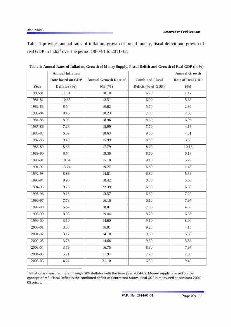
Table 1 provides annual rates of inflation, growth of broad money, fiscal deficit and growth of

real GDP in India4 over the period 1980-81 to 2011-12.

Table 1: Annual Rates of Inflation, Growth of Money Supply, Fiscal Deficit and Growth of Real GDP (in %)

Year

Annual Inflation

Rate based on GDP

Deflator (%)

Annual Growth Rate of

M3 (%)

Combined Fiscal

Deficit (% of GDP)

Annual Growth

Rate of Real GDP

(%)

1980-81 11.51 18.10 6.79 7.17

1981-82 10.85 12.51 6.00 5.63

1982-83 8.54 16.62 5.70 2.92

1983-84 8.45 18.23 7.00 7.85

1984-85 8.02 18.96 8.60 3.96

1985-86 7.28 15.99 7.70 4.16

1986-87 6.89 18.63 9.50 4.31

1987-88 9.49 15.99 8.80 3.53

1988-89 8.33 17.79 8.20 10.16

1989-90 8.54 19.36 8.60 6.13

1990-91 10.64 15.10 9.10 5.29

1991-92 13.74 19.27 6.80 1.43

1992-93 8.86 14.81 6.80 5.36

1993-94 9.98 18.42 8.00 5.68

1994-95 9.78 22.39 6.90 6.39

1995-96 9.13 13.57 6.30 7.29

1996-97 7.78 16.16 6.10 7.97

1997-98 6.62 18.01 7.00 4.30

1998-99 8.05 19.44 8.70 6.68

1999-00 3.10 14.60 9.10 8.00

2000-01 3.38 16.81 9.20 4.15

2001-02 3.17 14.10 9.60 5.39

2002-03 3.73 14.66 9.30 3.88

2003-04 3.76 16.75 8.30 7.97

2004-05 5.71 11.97 7.20 7.05

2005-06 4.22 21.10 6.50 9.48

4 Inflation is measured here through GDP deflator with the base year 2004-05. Money supply is based on the

concept of M3. Fiscal Deficit is the combined deficit of Centre and States. Real GDP is measured at constant 2004-

05 prices.


Page No. 12 W.P. No. 2014-02-04

2006-07 6.42 21.72 5.10 9.57

2007-08 6.02 21.38 4.00 9.32

2008-09 8.45 19.34 8.30 6.72

2009-10 6.07 16.85 9.30 8.59

2010-11 8.82 16.09 6.90 9.32

2011-12 8.23 13.23 8.10 6.21

Source: RBI, Handbook Of Statistics on Indian Economy2012-13

We can see from the table that the first episode of deliberate disinflation during this

period started in 1980-81 when inflation rate was 11.51%, growth of money supply was 18.10%

and the fiscal deficit was 6.79%. RBI cut the growth of broad money to 12.51% and government

cut the fiscal deficit to 6% in 1981-82 as a result of which inflation rate fell to 10.85%5. In the

next year 1982-83, the government continued with the policy to reduce the fiscal deficit to 5.70%

but RBI relaxed the growth of broad money to 16.62%- still less than initial 18.10% . The

inflation rate further fell to 8.54%. In 1983-84, the fiscal deficit was increased back to 7%

(marginally higher than the initial level) and the growth of money supply was restored to

18.23%. Inflation rate dropped marginally to 8.45%. Thus, the first episode of deliberate

disinflation can be taken as 1980-81 to 1983-84, because the growth rate of real GDP also

returned from 7.17% in 1980-81 to 7.85% in 1983-84. If we take the growth of potential output

as the average of these two end-points, i.e. 7.51%, we can get the Sacrifice Ratio in this

disinflation episode to be 2.11, implying that the society incurred the cost of 2.11% of a year’s

potential output to reduce the inflation rate by 1 percentage point.

The second episode of deliberate disinflation though aided by some favorable supply

shocks (RBI 2002a) is during the period 1998-99 to 2003-04. In 1998-99, RBI was also

effectively made autonomous from the Central Government. The inflation was high at 8.05%,

growth of broad money was at 19.44% and fiscal deficit was at 8.70% of GDP. RBI started

cutting down the growth rate of money supply and brought it down to 16.75% in 2003-04.

Subsequently, the inflation came down to 3.76% in 2003-04. This episode presents an

opportunistic disinflation policy by RBI because the global factors were initially favorable (RBI

2002a). Again following the same method of taking the average of the end-point growth rates of

5 It may be noted that during this period, RBI was not autonomous from the government.


Page No. 13 W.P. No. 2014-02-04

real GDP as the growth of potential output, the Sacrifice Ratio for this second period turns out to

be 1.84.

The third episode is not an episode of disinflation but deliberate inflationary policies and

covers the period from 2004-05 to 2008-096. Inflation was at 5.71% in 2004-05 and rose to

8.45% by 2008-09. While there was a fiscal tightening, RBI increased the growth of money

supply from 11.97% in 2004-05 to 19.34% in 2008-09. During this period of inflation, growth of

real GDP increased and reached the peak of 9.5% in 2006-07. The potential output growth

during the period as per the average of the two-end point growth was 6.89%. Therefore, the

Sacrifice Ratio during this inflationary episode would be 2.81, implying that by incurring the

cost of 1 percentage point of more inflation, the society gains 2.81% more output that may result

in reduced unemployment and hence reduced poverty proportion.

The above discussion clearly brings out that the direct approach for calculating the

Sacrifice Ratio results in the ratio differing with episodes. Moreover, inflationary episodes can

also be identified with the deliberate easy monetary policy and the Sacrifice Ratio in such cases

can also be calculated and meaningfully interpreted for developing countries like India. Finally,

the Sacrifice Ratio in India from episode to episode moves in a relatively narrow range of 1.8 to

2.8 and is of credible magnitude compared to whatever international experience and estimates

are available (See Kapur & Patra, 2003, Table 1).

Turning to the regression based approach to estimate the Sacrifice Ratio for India, we

must note several concerns raised for such estimates in our discussion in the previous two

sections. Estimates based only on the aggregate supply curve may not truly reflect the Sacrifice

Ratio because the latter captures the phenomenon on the locus of the short-run equilibria

between shifting DAS as well as DAD. Therefore, the variables shifting both DAS and DAD

should be considered while estimating the Sacrifice Ratio. The equations considered for the

estimation represent the solution of DAS and DAD functions for the short-run equilibrium values

of π and the percentage output gap. In simplified linear form, these equations would be:

6 Again in this case, the end-point coincides with the global financial crisis, but it would only depress the Sacrifice

Ratio marginally.


Page No. 14 W.P. No. 2014-02-04

π = �1π-1 + �2 (π-1 – π-2) + �3 gMS + b4 ∆ (FD/GDP) +�5 (Y-1 – Y*)/Y* + b6 ge + b7 πus + b8(gY – gY*) ------------------- (7)

(Y – Y*)/ Y* =�1π-1 + �2 (π-1 – π-2) + �3 gMS + a4 ∆ (FD/GDP) +�5 (Y-1 – Y*)/Y* + a6 ge + a7

πus + a8(gY – gY*) ---------- (8)

Where, FD is the combined Fiscal Deficit and GDP is at current market prices and the rest of the

variables are as defined earlier. Here, we are taking the expected inflation to be the previous

year’s inflation (π-1) following Anderson & Wascher (1999). Now, the equations (7) and (8)

would closely reflect short-run equilibrium values of π and percentage output gap as a function

of exogenous variables including growth in money supply. The equations (7) and (8) would

provide the Sacrifice Ratio as a ratio of the coefficients of gMS in the two equations. The short

run Sacrifice Ratio is given by (a3/b3). However, the long-run Sacrifice Ratio is [(a3/(1-a5)] /

[b3/(1-b1)].

In order to obtain the estimates of equations (7) and (8), we first need to measure the

percentage output gap from the potential output. This is obtained by fitting a log-linear trend to

the data. Based on the scatter of real GDP, we have considered trend-breaks at 1991-92 and

2003-04 in the series and obtained the following estimate of the spliced regression on LnY:

�� t = 13.54+0.0500t + 0.0084D1 (t-12) + 0.0227D2 (t-24)………… (9)7 (t-values) (1606) (50.13) (5.20) (10.94) Adjusted R-squared= 0.9993; Residual standard error= 0.0146 on 28 degrees of freedom; All the parameter estimates are statistically significant at 1% level.

Where t=12 for year 1991-92; and t=24 for year 2003-04. D1 and D2 are dummy variables such that –

D1 = �0, 1 ≤ ! ≤ 111, 12 ≤ ! ≤ 32

D2 = �0, 1 ≤ ! ≤ 231, 24 ≤ ! ≤ 32

From equation (9), we get the estimate of the trend level of output (Yt*) and hence the output gap

= (Yt – Yt*)/ Yt*.

7 It is interesting to see that this trend equation (9) implies annual compound growth of 5.12% during 1980-81 to

1991-92; 6.01% during 1991-92 to 2003-04; and 8.44% during 2003-04 to 2011-12. There has been a continual and

substantial acceleration in growth of real GDP in India.


Page No. 15 W.P. No. 2014-02-04

Now, we turn to the estimates of equations (7) and (8) above. Table 2 presents these estimates.

Table 2: Estimates of Equations (7) and (8) for India, 1980-81 to 2011-12

Variables Equation (7) on π Equation (8) on (Y – Y*)/ Y*

Coefficient t-value p-value Coefficient t-value p-value π-1 0.5926** 3.822 0.000 -0.0748 -0.804 0.429

π-1 – π-2 -0.1414 -1.237 0.228 -0.0061 -0.089 0.930

gMS 0.1045 1.221 0.234 0.1529** 2.979 0.007

∆ (FD/GDP) -0.2135 -0.900 0.377 0.0514 0.362 0.721

(Y-1 – Y*)/Y* -0.0537 -0.261 0.796 0.3998** 3.238 0.004

πtus 0.1888 0.949 0.352 0.0902 0.756 0.457

ge 0.0578 1.211 0.238 0.0070 0.245 0.808

gY – gY* -0.1371 -0.719 0.479 0.5853** 5.115 0.000

Adj. R-square 0.954** 0.424** Res. Std. Error 1.722 on 24 DF 1.033 on 24 DF Note: ** significantly different from zero at 1% level.

It can be seen from Table 2 that several variables in the two equations are statistically not

significant and the corresponding t-values are less than unity. However, the overall fit of the

regression is good in both the cases. It is, therefore, possible to get a better fit in terms of

adjusted R2 by dropping insignificant variables one by one in the step-wise regression. Finally,

the acceptable regression estimates that emerged are presented in Table 3.

Table 3: Estimates of the Best Fit of Equations (7) and (8) for India, 1980-81 to 2011-12

Variables Equation (7) on π Equation (8) on (Y – Y*)/ Y* Coefficient t-value p-value Coefficient t-value p-value π-1 0.5779** 4.082 0.000 -- -- --

π-1 – π-2 -0.1464 -1.324 0.196 -- -- --

gMS 0.1247*** 2.462 0.020 0.1464** 4.106 0.000

∆ (FD/GDP) -- -- -- -- -- --

(Y-1 – Y*)/Y* -- -- -- 0.4258** 4.207 0.000

πtus 0.2096 1.129 0.269 -- -- --

ge 0.0584 1.513 0.142 -- -- --

gY – gY* -- -- -- 0.5707** 5.555 0.000

Adj. R-square 0.957** 0.503** Res. Std. Error 1.667 on 27 DF 0.9596 on 29 DF Note: ** significant at 1% level; *** significant at 5% level.


Page No. 16 W.P. No. 2014-02-04

From the estimates of the coefficients of gMS given in Table 3, we can calculate the

Sacrifice Ratio for India since both the coefficients are statistically significant. The estimate for

the Sacrifice Ratio turns out to be (0.1464/0.1247) = 1.2 in the short-run; and [0.1464/0.5742) /

(0.1247/0.4221)] = 0.9 in the long-run8. The short-run ratio is higher than the long-run ratio

because the ratio is calculated for one percentage point reduction in the growth of money supply

(other things remaining the same). As time passes, expected inflation falls leading to positive

effect on output and negative effect on inflation. Therefore, the Sacrifice Ratio in the long-run is

likely to be lower than in the short-run for the same initial reduction in growth of money supply.

The regression approach estimates a constant and unique Sacrifice Ratio for an economy

as an average applicable over the entire period under consideration. On the other hand, the direct

approach allows the Sacrifice Ratio to vary across different episodes of disinflation and inflation.

However, the regression approach allows us to estimate the Sacrifice Ratio for the monetary

policy interventions by holding all other relevant factors constant. The regression approach is,

therefore, likely to provide more conservative estimates of the Ratio. In case, our interest is to

get separate estimates of the Ratio for episodes of disinflation and inflation, the direct approach

is the only alternative. For India, it shows the ratio varying by episodes of disinflation from 1.8

to 2.1; and for the episode of inflation to be 2.8.

8 As an alternative method to estimate the Sacrifice Ratio through the regression approach, we

may consider equations (5) & (6) above following Chand (1997). The estimates of the two equations are:

(π - π-1) = 0.5812 [gYP – (π-1+ gY* )…………………………………. (5’) t-value: (4.79); Adj. R-square= 0.4065

gY – gY* = 0.4188 [gyp – (π-1+ gy*)……………………………........... (6’) t-value: (3.45); Adj. R-square = 0.2541

Both these estimates are significant at 1% level. Moreover, since both the estimated coefficients add up to one, the requirement of internal consistency is met. The Sacrifice Ratio in this framework works out to be (0.4188/0.5812)= 0.72. However, it should be noted that this estimate should be interpreted to say that the difference of actual growth of output from the growth of potential output would fall by 0.72 percentage points when actual inflation declines by 1 percentage point. This estimate is close to the one obtained above for the long-run (0.86), but since no other factor is held constant, it cannot be considered only the result of any deliberate monetary policy.


Page No. 17 W.P. No. 2014-02-04

V. Cost of Inflation in India

It is necessary to consider the cost of inflation in India in view of the Sacrifice Ratio

estimates. Thus, reducing the long-run inflation say, from 8% to 5%, would entail the social cost

of sacrificing 5.4% to 6.3% of potential output as per our estimates in the previous section.

By now it is very well accepted that long term anticipated inflation has hardly any serious

cost on the society and that unanticipated inflation largely has distributional costs in the society

(Dornbusch, Fischer & Startz, 2012; Mankiw, 2010). Barro (1995) and Fischer (1993) argue that

so long as inflation is moderate, say less than 10% p.a., it does not hurt the long-term growth of

the economy. On the other hand, Chopra (1988); Motley (1994); Paul et al. (1997); and

Chaturvedi et al. (2009) find negative impact of inflation on growth in a cross-country and Indian

context. Chaturvedi et al. (2009) provide the latest evidence and their study period is 1989 to

2003. It, therefore, requires examining this issue with latest data for India. This is because if

reducing inflation rate from say 8% to 5% does not have any positive impact on the long-term

growth, it may not be worth sacrificing about 6% of potential output to achieve such a reduction.

If, on the other hand, it raises the long-term growth substantially, it may be worth undertaking

reduction of inflation.

In order to examine this relationship, we have fitted the log-linear trend on the GDP

deflator from which we derive the inflation rate. By observing the scatter, we identified two

trend-break points: 1998-99 when RBI was given effective autonomy; and 2004-05 when UPA-1

came to power with an explicit commitment to double agricultural credit every three years. The

fitted regression equation is -

Ln (GDPdef.) = 2.7463 + 0.0867 t – 0.0560 D1 (t-19) + 0.0376 D2 (t-25) -------------------- (10)

t-values: (286.2) (108.7) (-18.94) (8.02)

Adjusted R-square = 0.999; Residual Standard Error = 0.0206 for 28 Degrees of Freedom.

D1 & D2 are dummy variables such that -

D1 = �0, 1 ≤ ! ≤ 181, 19 ≤ ! ≤ 32


Page No. 18 W.P. No. 2014-02-04

D2 = �0, 1 ≤ ! ≤ 241, 25 ≤ ! ≤ 32

All parameters are significant at 0.1% level.

Thus, there are three distinct phases of inflation experience in the country: (i) 1980-81 to

1998-99, when the trend rate of inflation was 9.06% p.a.; (ii) 1998-99 to 2004-05, when the trend

rate of inflation was 3.02% p.a. and (iii) 2004-05 to 2011-12, when the trend rate of inflation was

7.07% p.a. From phase (i) to (ii), there was a conscious effort to bring down the long-run

inflation in the economy by almost 6 percentage points. It can be seen from the Table 1 above

that RBI after becoming autonomous in 1998-99 attempted to cut the growth of money supply

substantially to achieve this, though its efforts were compounded and facilitated by global factors

(RBI, 2002a). On the contrary, from phase (ii) to (iii), there was a conscious effort to raise the

inflation rate in the economy by almost 4 percentage points through systematic efforts to raise

the growth of money supply (see Table 1 above). In order to examine the broad effects of such

sharp long-term deflation and inflation on the output growth in the economy, we also fitted log-

linear trend on GDP at 2004-05 prices taking the same trend-break points as in the case of GDP

deflator. The fitted regression equation is -

Ln Yt = 13.52 + 0.0533 t + 0.0102 D1 (t-19) + 0.0192 D2 (t-25) --------------------------- (11)

t-values: (1556) (73.8) (3.81) (4.52)

Adjusted R-square = 0.9989; Residual Standard Error = 0.0187 for 28 Degrees of Freedom.

D1 and D2 are dummy variables with same definition as in equation (10).

All parameters are significant at 0.1% level.

These estimates show that during the same three phases identified above on the basis of

inflationary trends, the trend growth of output turned out to be: (i) 5.47% p.a. during 1980-81 to

1998-99; (ii) 6.55% p.a. during 1998-99 to 2004-05; and (iii) 8.61% p.a. during 2004-05 to 2011-

12. Thus, the output growth consistently and continually accelerated across the three phases

while the trend rate of inflation fell sharply between phases (i) and (ii); and sharply increased

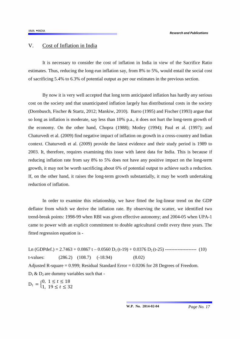
between phases (ii) and (iii). Figure 2 provides the graphs of the fitted log-linear trend rates and

actual annual growth for both GDP deflator and real GDP by years.


Page No. 19 W.P. No. 2014-02-04

If we consider the period only up to 2004-05 as was done by Chaturvedi et al. (2009), it would

appear that inflation and growth of output are negatively related. In other words, a reduction of

inflation by about 6 percentage points leads to an increase of about 1 percentage point in long-

term output growth, or a reduction of 1 percentage point in trend rate of inflation would lead to

about 0.18 percentage points increase in the long-term annual growth rate.

Figure 2: Fitted Trend Rates and Actual Annual Inflation Rates and Growth Rates in India

However, after 2004-05, the experience in India tells a different story. An increase of

about 4 percentage points in trend rate of inflation between phases (ii) and (iii) is accompanied

by an increase of more than 2 percentage points in the long-term growth rate of output. Thus,

inflation and growth of output are positively related. In this case, there are no particular benefits

of attempting to reduce trend rate of inflation. On the contrary, raising the trend rate of inflation

by 1 percentage point may result in increasing the long-term growth by 0.51 percentage point.

Such contradictory evidences would obviously make the regression results covering the entire

period less reliable and even statistically less significant.

0

2

4

6

8

10

12

0

2

4

6

8

10

12

19

80

-81

19

81

-82

19

82

-83

19

83

-84

19

84

-85

19

85

-86

19

86

-87

19

87

-88

19

88

-89

19

89

-90

19

90

-91

19

91

-92

19

92

-93

19

93

-94

19

94

-95

19

95

-96

19

96

-97

19

97

-98

19

98

-99

19

99

-00

20

00

-01

20

01

-02

20

02

-03

20

03

-04

20

04

-05

20

05

-06

20

06

-07

20

07

-08

20

08

-09

20

09

-10

20

10

-11

20

11

-12

Estimated Growth Rate Estimated Inflation Rate

Actual Growth Rate Actual Inflation Rate


Page No. 20 W.P. No. 2014-02-04

In this context, the finding of Dholakia & Sapre (2012) about the length of period

considered by people to form price expectations in the country become very relevant to examine

costs or benefits of changes in the long-term inflation trend in terms of output growth. Dholakia

& Sapre (2012) find that people consider the experience of last four years to form inflationary

expectations in India. Therefore, the permanent benefits of reducing long-term inflation rate

would be felt only after 4-5 years. Thus, reduction of trend rate of inflation by about 6

percentage points during 1998-99 to 2003-04 would show the real impact on the long-term

growth of output after 2004-05 and continue up to 2008-09, because there is an upward shift in

the trend rate of inflation around 2004-05. A sharp increase in trend rate of inflation after 2004-

05 similarly would show its negative impact on growth after 4-5 years, i.e. after 2008-09 or

2009-10. If we examine the growth experience in recent years, adjust for the external and

exogenous factors and relate it to the inflation rate before 4-5 years, we would corroborate the

substantial negative influence of inflation on growth9.

VI. Concluding Remarks

Thus, the cost of high inflation is the sacrifice of substantial growth in the long-term; and

the benefit of disinflation is a sizeable gain in the long-term growth in the economy. However,

disinflation is not costless as we have seen through the Sacrifice Ratio of about 0.9 to 2.1 in the

short to intermediate period. On the other hand, the long-run gain in the growth rate per

percentage point reduction in inflation rate is only 0.5. If, therefore, a 3 percentage point

reduction in trend rate of inflation is targeted, it would start positively impacting the growth after

about 4-5 years and would take nearly 2 to 4 additional years to recover the cost of achieving it

without discounting for the society. It is a moot question whether the political priorities and

commitments would remain the same over such a long period. If not, it may take longer to

recover the cost of disinflation. RBI needs to seriously consider achieving disinflation at a

relatively high cost compared to the gain from it with respect to the time element involved.

9 This is because Chaturvedi et al. (2009) have conclusively established that the relationship between inflation and

growth is not bi-directional, but uni-directional- from inflation to growth only. This is particularly true for Asian

countries.


Page No. 21 W.P. No. 2014-02-04

On the other hand, raising the trend inflation marginally appears to be politically a good

option, because the gains are immediate in terms of higher growth, more employment and

poverty reduction, and the costs in terms of lower long-term growth are in the future, perhaps for

the next government to face. On account of data limitations, strong evidence on the hypothesis of

growth of output leading to expansion in employment leading to poverty reduction in India is not

available. However, output elasticity of employment and employment elasticity of poverty

proportion can be calculated from the readily available data from the NSS Surveys on

employment –unemployment situation and on consumer expenditures undertaken in 1993-94

(NSS 43rd Round) and 2011-12 (NSS 63rd Round). The output elasticity of employment works

out to + 0.1882; employment elasticity of poverty proportion works out to (-) 3.3643; and output

elasticity of poverty proportion works out to (-) 0.633110. These figures do provide broad support

to the hypothesized relationship between higher growth and more employment and poverty

reduction in India. It is then possible to argue a case for an inflationary policy through the

Sacrifice Ratio to incur permanent cost of inflation to gain temporarily in terms of employment

creation and poverty reduction. Thus, pure cost-benefit analysis of disinflationary versus

inflationary policies may favor the latter over the former depending on the magnitudes of the

Sacrifice Ratio and the long-term costs / benefits of disinflation / inflation in an economy.

References:

Andersen, P. S. and W. L. Wascher (1999). ‘Sacrifice ratios and the conduct of monetary policy

in conditions of low inflation’, BIS Working Papers, 82, Bank for International Settlements.

Ball, L. N. (1994). ‘What Determines the Sacrifice Ratio?’ in N.Gregory Mankiw (ed.) Monetary

Policy, University of Chicago Press, pp.155 – 193.

Barro, R. (1995). ‘Inflation and Economic Growth’, NBER Working Papers 5326, National

Bureau of Economic Research, Inc.

Chand, S.K. (1997), Nominal Income and the Inflation-Growth Divide, IMF Working

Paper WP/97/147.

10

All these are arc elasticity estimates calculated from two end points.


Page No. 22 W.P. No. 2014-02-04

Chaturvedi, V., B. Kumar and R. H. Dholakia (2009). ‘Inter-relationship between Economic

Growth, Savings and Inflation in Asia’, Journal of International Economic Studies, No. 23,

March, pp. 1–22.

Chopra, S. (1988). Inflation, Household Savings and Economic Growth, Ph.D. thesis, M.S.

University of Baroda, India.

Dholakia, R. H. (1990). ‘Extended Phillips curve for the Indian economy’, Indian Economic

Journal, 38 (1), pp. 69-78.

Dholakia, R. H. and A. Sapre (2012). ‘Speed of Adjustment and Inflation- Unemployment

Tradeoff in Developing Countries - Case of India’, Journal of Quantitative Economics, 10(1),

pp. 1-16.

Dornbusch, R. and S. Fischer (1990). ‘Macroeconomics’, 5th Edition, New York, McGraw Hill

(India) Pvt. Ltd.

Dornbusch, R., S. Fischer and R. Startz (2012). ‘Macroeconomics’, 10th Edition, New Delhi,

Mcgraw Hill Education (India) Pvt. Ltd.

Fischer, S. (1993). ‘The role of macroeconomic factors in growth’, Journal of Monetary

Economics, 32 (3), pp. 485-512.

Kapur M. and M. D. Patra (2003). ‘The Price of Low Inflation’, RBI Publications, 33952,

January.

Mankiw, N. G. (2010). ‘Macroeconomics’, 7th Edition, New York, Worth Publishers.

Motley, B. (1994). ‘Growth and Inflation: A Cross-Country Study’, CEPR Publication No. 395,

Centre for Economic Policy Research, Stanford University, March.

Paul, S., C. Kearney and K. Chowdhury (1997). ‘Inflation and economic growth: a multi-country

empirical analysis’, Applied Economics, 29(10), pp. 1387-1401.

Reserve Bank of India (2002). Report on Currency and Finance, 2000-01.

—— (2002a), Annual Report, 2001-02.

—— (2013), Handbook of Statistics on Indian Economy 2012-13.

Sacrifice Ratio and Cost of Inflation for the Indian Economy · Sacrifice Ratio and Cost of...

Documents

Transcript of Sacrifice Ratio and Cost of Inflation for the Indian Economy · Sacrifice Ratio and Cost of...