AD-RI59 926 ESTINTION OF POPULTION PROPORTION ND OF

1/1PROBABILITIES OF NISCLRSSIFICR..(U) MRYLAND UNIYCOLLEGE PARK DEPT OF MANAGEMENT SCIENCES AND ST.. N

RUNCLASSIFIED N L JOHNSON ET AL. AUG 95 UM/MSS/85/7 F/G 12/1 N

inEsh~hEh

Ii

* 111111.0

n JjM2

0-

- -,It.-,-u. -

11111 -i 11.2"

I 1.25 1114I,6 .

MICROCOPY RESOLUTION TEST CHART

NATIONAL gIJUAU OF STANOaAoS IS A

*. . . . . ..o ...|-, %4

I' .

A[. ~

CID* N

0Y)

In* I

ESTIMATION OF POPULATION PROPORTION AND OF PROBABILITIES OF

( MISCLASSIFICATION FROM IMPERFECr BINOMIAL DATA BY CavPARISON WITH

RESULTS OF A STANDARD METHOD OF KNOWN INPERFECTION

Norman L. Johnson and _nel KotzUniversity of North Carolina /University of MarylandChapel Hill, North Carolina V/ College Park, Maryland

August 1985

OT2 686~

8A

document has been approved

8for Public release and Sale; its• L distribution is unlimited.

i!?i~ ~ 8 8 9 0 6:

ESTIMATION OF POPULATION PROPORTION AND OF PROBABILITIES OF

MISCLASSIFICATION FRCM IMPERFECT BIN0LAL DATA BY CCtPARISON WITHI

RESULTS OF A STANDARD METHOD OF KNOWN IMPERFECTION

Norman L. Johnson and Sanuel KotzUniversity of North Carolina University of MarylandChapel Hill, North Carolina College Park, Maryland

ABSTRACT: Observations from inspection by a testf thod and a standard

method are combined to provide estimators of population proportion, and

of probabilities of misclassification for the test method. Results of

Hochberg and Tenenbein (1983) and of Albers and Veldman (1984) are

extended to the case where the standard method is not perfect, but its

misclassification probabilities have known values. Both moment and maxinum

likelihood estimators are considered and some asymptotic properties of the

resulting estimators are compared. .- o'

Key Words and Phrases: Binomial distribution; information matrix;

inspection errors; maximum likelihood; method of moments; statisticaldifferentials.

/

1. INTRODUCTION

Suppose we have a large population, containing an unknown proportion,

P, of individuals possessing a certain characteristic, which we will

call 'nonconformance'. In a random sample, of size n, from this population,

the distribution of the number, X, say, of nonconforming individuals

will be binomial with parameters n,P so that

-. in ,x (l_p)n-,Pr[X-x] = (.) (xf= 0,1,...,n).

We will represent this, symbolically, as

X - Bin(n,P) , where - denotes "is distributed as".

If the individuals in the sample of size n are examined by an

imperfect measuring device, which detects actual nonconformance with

probability p, and (incorrectly) 'detects' nonconformance, when the

individual is really not nonconforming, with probability p', then the

distribution of Z, the number of individuals declared to be nonconforming,

as a result of this inspection, will be binomial with parameters n,

Pp+ (l-P)p' . It is clear that the only parameter that can be estimated

from observations on values of Z in independent samples is Pp + (l-P)p',%

Various methods have been suggested for obtaining data from which

estimates of P, p and p' can be derived (e.g. Albers and Veldman (1984),

. Johnson and Kotz (1985)). Tenenbein (1970) suggested additional inspection

of part of the sample by a perfect measuring device (for which pal and

p'=O) and utilizing the resultant data. This method has been extended by

Hochberg and Tenenbein (1983) to allow for inspection of a further sample,

.' of size ns, say, by the perfect measuring device (S).

5%

',

2

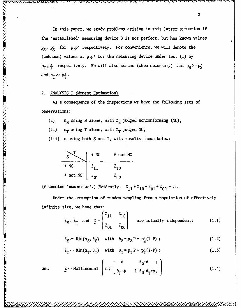
In this paper, we study problems arising in this latter situation if

the 'established' measuring device S is not perfect, but has known values10

PS' ,P for p,p' respectively. For convenience, we will denote the

(unknown) values of p,p' for the measuring device under test (T) by

pT pi respectively. We will also assume (when necessary) that PS > > p '

and pT >> I

2. ANALYSIS I (oment Estimation)

As a consequence of the inspections we have the following sets of

observations:

(i) n S using S alone, with ZS judged nonconforming (NC),

(ii) nT using T alone, with ZT judged NC,

(iii) n using both S and T, with results shown below:

ST # NC # notNC

# NC ZII Z0

# not NC Z01 ZOO

(# denotes 'number of'.) Evidently, Z +Z +Z+01 Z00 n.

Under the assumption of random sampling from a population of effectively

infinite size, we have that:

Zll ZlO

ZS, ZT and Z - are mutually independent; (1.1)Z 01 Z0 0

- Bin(ns, 6) with es=psP+ p'(1-P) ; (1.2)

ZT- Bin(nT,eT) with eTpTP4 p+(l-P) ; (1.3)

€ es-F [ 8T 'S%+Pand Z '-Multinomial n; 6S (1.4)

-" T - .,. "' .T

3

with = psTP + p p+(1-P) where, denotes "is distributed as".Recall that PS and p have known values, and P is the (unknown)

proportion of NC individuals in the population.

Hence

(n + n)8 S = ZS + Z10 + Zll Bin(ns+n, es) (2.1)

(nT + n)6T = ZT + Z01 + Z11 - Bin(nT+n, OT) (2.2)

= Z11 Bin(n,o) (2.3)

so that es 6 T and € (as defined in (2.1)-(2.3)) are unbiased estimators

of 6s, eT and 0 respectively.

Hence P = (pS-pI)( % (3.1)

is an unbiased estimator of P. Although the estimators

- (6s -P)(- 0T) (3.2)

and = (ps-es)-l(ps'T- ) (3.3)

are not unbiased estimators of PT and p+ respectively, the biases should not

be large if sample sizes are adequate (see the example later in this section).

The variance-covariance matrix of the random variables in (2.1)-(2.3) is

(ns+n) S(l-eS) n(0-60sT) no(1-e S )

Var((nS+n) S, (nr+n) 'T,n)= n(.-0S0T) (n.T+n)0T(1-0T) nO(l-eT) (4)

n0l -eOS) n ( 1 -6 T) n ( 1-o )

Hence (cf. (3.1))

Var(P) = (ns+n)'(ps-p )2e (1- 8 ) (5.1)

and, using the method of statistical differentials (see, e.g. Johnson and

Kotz (1969, Chapter 1, Section 7.5))we obtain, after some algebraic manipulation:

- ~ ~ ~ ~ ~ ~ ~ ~ ~ ~ ~ ~ 7 -- , .. l - V- *- ~ .~~ a . -.- S- -

4

var (~pT (P P-2 p l)-2[ n'(lJ )2 ntJ )-pS (1T) rtn -1PA2T('-T)PT

-2(nS+n)- 1 (l-eS )-n(nt+n) -1pS(,eOSeT)}pT1 + (nS+n)- 1 sle) 52

An approximate expression for var(q) is obtained from (5.2) by

replacing pT by p+. and P by (l-P), and interchanging p and p .

An approximate formula for the bias of -Tis

E[pTJ - pT pT - a(O-p) - -a~sp eT (6)1e- ) (6 -P')(O-P' OT)

which, after some reduction, gives a proportional bias (i.e. 100(bias)/pT%)

1OO{n~pl(l-OS) + n(l-pl) 06 S T 7

(n+n) (nT+n) (OS-P ) 2(OeT)

From (1.1)-(l.4)

6-,= (p -p;)P; ";p eT = P(SP)

and -e Se6T = P(l P)(P 5-P;)(Pp-p) , so

the approximate proportional bias (7) is

1OO(n..~p(l-e5 ) + n(l-p )e5 1 (IP(p j 70 (7)'

(nS+n) (nT+n)P 2 (pS-PA) 2

which is positive and (since Pi < PT less than

100 Gfl- L 7 (8)*(nS+n)P 2(p5-pa) I

5

where

G = p(l-e s ) + _ -p)e5 (9)nr+n 1p s,9

which lies between p(l-0 S) and (1-p ) S .

Example. Using as 'typical' values of the probabilities pS, pS and P the values

0.9, 0.1 and 0.1 respectively we find that

G = (nT+n)- 1(0.08 2nT + 0.162n)

(so that G lies between 0.082 and 0.162) and the approximate proportional bias

of PT is between 0 and 1406.25 G(ns+n) -1% . Note that the upper limit is

less than 227.8 (ns+n) 1%, so if ns+n> 100 the approximate proportional bias

is less than 2.28%. The next section contains a numerical assessment of

formula (5.2), without specifying values of PT and p+.

3. Some Numerical Approximations

Utilizing the reasonable assumption that p,>> p , and neglecting

terms in pI and p 2 in the numerator of (5.2) we find

2 2(p ?)-2 (i) 20(1-0s) eS(-es)Var(k) P ~T P~p-~ 2 - S + (10)

,IP; npT (nS+n)pT ns+n

Taking pS = 0.9, p = 0.1 so that 6S = 0. 8P+0. and = 0.9 PTP + 0.1 p(l-P)

we obtain from (10)

2 [ + 0.lp+(1-P)}{1-0. 9pTP- 0.lp+(1-P)}Var(pT) PT 2

0.64PL n pT

(0.8P+0.1)(0.9-0.8P) - {1.8pP + 0.2p+(l-P)(0.9-0.8P)PT1

n

, . ., , 7 % . . . . : '% ' . ' - -. .. .. . ., . .- . . .. _ ..- .. _ .. -n -.+.-.n

o r, te " * " 'r ' " - e , - . . , - • . . " . - , - . - . - o - . - . - .

6

Now taking P = 0.1, we find

2 - oP~pp-0~~P+~l ___var( ) -

-pT sn0.1476 PT (1i)

0.0064 L p nS+n PTj

14.375 (pT+P+){l_0.09(PT+p+)} _ 23.06 p+ (12)n ns+n PT

Since 0.0 9 (PT+p+){1-0.0 9 (PT+p+)} < .1 (because 0.09(PT+p ) < 1) the right hand

side of (6) is less than

(0.0256n) < 39.1 n

In the next section we will compare the asymptotic variances and covariances

of S, T and P with those for maxinmu likelihood estimators 8S' 6T and P of eS.

eT and P respectively.

4. ANALYSIS II (Maximum Likelihood Estimators)

The likelihood function of ZS, ZT and Z is[ZS I nT ][ZIZ',Z,Z00 Z S l ns-ZsZ0ZO

[S ] J lzz' ]es(1-eS cZl1(es- )Zl°(eT-¢) 01z-es-T+)o

Equating derivatives of the log-likelihood to zero gives the following equations

for e SD and 0:

Zs ns-Zs Zlo Z 00-+ --- - (13.1

8 S 1-6 S 8S€ 1-8s-T+¢

ZT nT-ZT Z01 Z00 -0 (13.2)eT 1- -e _6+ 4OT T T 1 S T

Zil Zl0 z01 ZA 0 0 (13.3)

0 es _0T- 1-eS-eT+

- --.. --,, .-. '- -- .- ." '..-.- .--.-v., ." -.'.' '..., . ..,.".....-""."-'-."".'".:.".."'."...............'.v'

7

* The informat ion matrix is

n f s n(l-6 T) n____ n(1l6 T)

8 s (1-6~ s -e-)le-T 1-0 Se (aS01es T+

1= nn n(1-65 ) n(l-e5 )

n~-T) fl1s) n~SeT(l eSe0T) +2eSeT"~

(14)

The determinant is

with y a 6 1e-6+ - W'0S0T (15)

and from the asymptotic variance-covariance matrix V we obtain

___ _________1 IfT 1 1 1 -- nT~ 1 +i1i

T 6S(I-eS) (ynS +6N )/-y+6)

* where N =nfS+flT+nl( total number of observations) and

6 = nN OS T(l-OS) (lTYnSnT

The NILE of P is

P = (P-' (e- (16)

The asymptotic efficiency of P (see (3.1)) is the same as that of apwhich is

1OO(n s fl)(y n S_ + 6N_ )/(Y+6) % (17)

8

Taking pS=pT=0.9 , p pIS =0.1=P and ns=nT=n (- N) we find

y=0.0184680 and 6=0.0653573, so (17) becomes

100(ns+n) (0.2203 ns-l+ 0.7797 N-1)

= 2(0.2203+0.2599) = 96.04%.

The asymptotic variance of the MLE $ is

6d2-l{nses-l(1-e S) +nTeT-1(1-BT )}+ €(e- )(eT-€)(l-s-T+O)var($) " 1 n 6+y

(18)

On the other hand, recalling that var( ) = n-l(1-0), we find for the

numerical values of the parameters used above, that the asymtotic efficiency

of the moment estimator 0 is

-19

100 x 0.0653573x0.09{0.91 - (2/3) xO.09x (0.18) -xO.82} + 0.09x O.09'x 0,730.09x 0.91 0.0653573 + 0.0184680)

100 x 0.0037449 + 0.0005322 62.30%0.0068653

The markedly lower asymptotic efficiency of 4 is associated with the fact

that it does not utilize the information on values of 6S and eT which is

available from the other (ns+nT) observations. Some support for this statement

comes from the asymptotic efficiency of @ if the values of S and eT are known.

This is

(es- ) (eT-O) (1-e-eT+O)100 x -S(19)

y(1-O)

With the numerical values of OS, eT and € which we have been using above this

would give an asymptotic efficiency of only 35.18%.

L.

.5I.

-0

9

S. CORRELATIONS

The asymptotic covariances between the MLE's6S and 6T' and between

esand $, are

CoV(sTl " N-1 6(4-eSeT)/(Y+6) (20)

and cov(0s,$) N- 1 6 0{nmT-l(l-4es-l) + 1-eS}/(y+6) (21)

Since 0 < eST < 0 < eS < 1, the covariances cannot be negative. It is

of interest to compare (20) wi,,h the covariance between the moment estimators

0S and 0T' which is

covos(OT) = n(ns+n)-1 (nT+(-1 ST) (22)

and (21) with the covariance between Sand , which is

cov(0s,4) = (ns+n) -l 0l_-se (23)

I Using our illustrative parameter values (ps=PT=0.9; p'=p'=0.1=P;

n=ns=nT) we obtain the following values for correlations:

corr(eS,eT) = 0.195; corr(OsM) = 0.475

corr(=S, T) 0.021; corr(8=,) " 0.S13

Note that if n=0 (and ns, nT > 0) then

corr(6S,eT) = corr(eS,eT) = 0.

Also, if ns=nT~=O (and n > 0) then

corr(0S,tT) = corr(St T) = (4-esT){eSeT(1es)(1-eT)}-

S(-- 0.390)

and

corr(est) = corr(esv) =[ -6s)/{Os(1

(= 0.147)

(Numbers in parentheses are values corresponding to pS=pT=0.09, p =p=0.I=P.

. o ° * .p, •. -., . -. . . . ...

Io

Acknowledgement

Dr. Samuel Kotz's work was supported by the U.S. Office of Naval Research under

contract N00014-84-K-0301.

REFERENCES

Albers, W. and Veldman, H.J. (1984) Adaptive estimation of binomial probabilities

under misclassification, Statist. Neerland., 38, 233-247.

Hochberg, Y. and Tenenbein, A. (1983) On triple sampling schemes for estimating

from binomial data with misclassification errors, Comnmun. Statist. - Theor.

Math., 12, 1523-1533.

Johnson, N.L. and Kotz, S. (1969) Distributions in Statistics: Discrete

Distributions, Wiley, New York.

Johnson, N.L. and Kotz, S. (1985) Some tests for detection of faulty inspection,

Statist. Hefte, 26, 19-29.

Tenenbein, A. (1970) A double sampling scheme for estimating from binomial data

with misclassification, J. Amer. Statist. Assoc., 65, 1350-1362.

-°2

,)".'%- . i( ,,', W" " Q"." ." ,€"q- .- . . ..... -. . ... . . . . . . . . . ......................

NONCLASSIFIEDSECUDITY CLASSIFCATION OF THIS PAGE A //"

REPORT DOCUMENTATION PAGEl. REPORT SECURITY CLASSIFICATION lb. RESTRICTIVE MARKINGS

Nonclassified2& SECURITY CLASSIFICATION AUTHORITY 3. DISTRI UUTIONIAVAI LABILITY OF REPORT

2b. OECLASSIFICATION/OOWNGRAOING SCHEDULE

4. PERFORMING ORGANIZATION REPORT NUMBER(S) S. MONITORING ORGANIZATION REPORT NUMBER(S)

UM/MSS/35/7Ga. NAME OF PERFORMING ORGANIZATION b. OFFICE SYMBOL 7. NAME OF MONITORING ORGANIZATION

Univ. of Maryland U.S. Office of Naval Researchk ADDRESS (City, State and ZIP Code) 7b. ADDRESS (City. State end ZIP Code)

Dept of Managenrent'and StatisticsUniveXrsity of MarylandCollege.Park, MD 20742 "

Se. NAME OF FUNOING/SPONSORING Sb. OFFICE SYMBOL 9. PROCUREMENT INSTRUMENT IDENTIFICATION NUMBER'ORGANIZATION (if applicable)

ONR N 00014-84-K-301Bc. ADDRESS (City. State and ZIP Code) 10. SOURCE OF FUNDING NOS.

Stat. and Probability Program PROGRAM PROJECT TASK WORK UNIT

Office of Naval Research ELEMENT NO. NO. NO. NO.

Arlington, VA 22217, InciudA mSecunt C ri ,oia,,Estimation of popula ion proportiin and of probabilities of meis-

classification from imperfect binomial data by comparison wtth result. of a standard method12. PERSONAL AUTHOR(S) of known imperfection"J(4SON. -N. L. and KTZ. Samuel13a. TYPE OF REPORT 13b. TIME COVERED 14. DATE OF REPORT (Yr.. ,Wo.. DayP 15. PAGE COUNT

TECHNICAL PROM 9/84 TO 9/85 August 1985 il pages16. SUPPLEMENTARY NOTATION

[17. COSATI CODES It SUBJE.CT TE RS Wt i . uer if.ecem er.mnd iden!tfy by btoh number

IELD GROUP SUB. GR. Dinomnal distriDUtiOn; information matri*; inspectionerrurs; maximum likelihood; method of moments; statisticaldifferentials.

19. ABSTRACT "(Continu. on reterse if n.ecemry and ideatify by block number)

Observations from inspection by a 'test' method and a standard method are combinedto provide estimators of population proportion, and of probabilities of misclassificatinnfor the test method. Results of Hochberg and Tenenbein (1983) and of Albers and Vetdman-(1984) are extended to the case where the standard method is not perfect, but itsmisclassification probabilities have known values. Both moment and maximum likelihoodestimators are considered and some asymptotic properties of the resulting estimators arecompared.

20. OISTRIBUTION/AVAILABILITY OF ABSTRACT 21. ABSTRACT SECURITY CLASSIFICATION

UNCLASSIFIED/UNLIMITEO K SAME AS APT. 0 OTIC USERS 0 Nonclassified

22a. NAME OF RESPONSIBLE INDIVIDUAL 22b. TELEPHONE NUMBER 22c. OFFICE SYMBOL,I rlude A res Code)

Samuel Kotz (301) 454-6805

DO FORM 1473, 83 APR EDITION OF 1 JAN 73 IS OBSOLETE. NONCLASSIFIEDSECURITY CLASSIFICATION OF THIS PAGE

.. eI

11-85

DTlC....... ..