Inequalities for -Norms that Sharpen the Triangle ...

The Journal of Geometric Analysis (2021) 31:4051–4073https://doi.org/10.1007/s12220-020-00425-y

Inequalities for Lp-Norms that Sharpen the TriangleInequality and Complement Hanner’s Inequality

Eric A. Carlen1 · Rupert L. Frank2,3 · Paata Ivanisvili4 · Elliott H. Lieb5

Received: 6 November 2019 / Published online: 25 May 2020© The Author(s) 2020

AbstractIn 2006 Carbery raised a question about an improvement on the naïve norm inequality‖ f + g‖p

p ≤ 2p−1(‖ f ‖pp + ‖g‖p

p) for two functions f and g in L p of any measurespace. When f = g this is an equality, but when the supports of f and g are disjointthe factor 2p−1 is not needed. Carbery’s question concerns a proposed interpolationbetween the two situations for p > 2 with the interpolation parameter measuring theoverlap being ‖ f g‖p/2. Carbery proved that his proposed inequality holds in a specialcase. Here, we prove the inequality for all functions and, in fact, we prove an inequalityof this type that is stronger than the one Carbery proposed. Moreover, our strongerinequalities are valid for all real p �= 0.

Keywords Lp space · Minkowski’s inequality · Convexity

This paper may be reproduced, in its entirety, for non-commercial purposes. Work partially supported byNSF grants DMS-1501007 and DMS-1764254 (E.A.C.), DMS–1363432 (R.L.F.), DMS–1856486 (P.I.),PHY–1265118 (E.H.L.).

B Rupert L. [email protected]

Eric A. [email protected]

Paata [email protected]

Elliott H. [email protected]

1 Department of Mathematics, Hill Center, Rutgers University, 110 Frelinghuysen Road,Piscataway, NJ 08854-8019, USA

2 Mathematisches Institut, Ludwig-Maximilans Universität München, Theresienstr. 39, 80333Munich, Germany

3 Mathematics 253-37, Caltech, Pasadena, CA 91125, USA

4 Department of Mathematics, University of California, Irvine, CA 92617, USA

5 Departments of Mathematics and Physics, Princeton University, Princeton, NJ 08544, USA

123

http://crossmark.crossref.org/dialog/?doi=10.1007/s12220-020-00425-y&domain=pdf

http://orcid.org/0000-0001-7973-4688

4052 E. A. Carlen et al.

1 Introduction andMain Theorem

1.1 Main Result

Since |z|p is a convex function of z for p ≥ 1, for any measure space, the L p unit ball,{ f : ∫ | f |p ≤ 1}, is convex. One way to express this is with Minkowski’s triangleinequality ‖ f + g‖p ≤ ‖ f ‖p + ‖g‖p. Another is with the inequality

‖ f + g‖pp ≤ 2p−1 (‖ f ‖p

p + ‖g‖pp), (1.1)

valid for any functions f and g on any measure space. There is equality in (1.1) if andonly if f = g and, in our main result (Theorem 1.1), we improve (1.1) substantiallywhen f and g are far from equal.

In 2006 Carbery [3] proposed several plausible refinements of (1.1) for p ≥ 2, ofwhich the strongest was

∫| f + g|p ≤

(

1 + ‖ f g‖p/2

‖ f ‖p‖g‖p

)p−1 ∫(| f |p + |g|p) . (1.2)

He proved that this inequality holds when f and g are characteristic functions of sets,but left the general case open. Our result provides the first proof of the inequalityproposed by Carbery.

The ratio � = ‖ f g‖p/2

‖ f ‖p‖g‖p, that appears in (1.2), varies between 0 and 1 and, there-

fore, the factor of (1+�)p−1 varies between 1 and 2p−1. Thus, (1.2), which we showto be true, is a refinement of (1.1).

In contrast to (1.1), there is equality in (1.2) not only when f = g, but also whenf g = 0. The extreme values 2p−1 and 1 of the factor of (1 + �)p−1 correspond tothese two cases of equality in (1.2).

Here, we propose and prove a strengthening of (1.2) in which � is replaced by thequantity

�̃ := ‖ f g‖p/2

(‖ f ‖p

p + ‖g‖pp

2

)−2/p

. (1.3)

By virtue of the arithmetic-geometric mean inequality we have �̃ ≤ � and therefore(1.2) with � replaced by �̃ is a stronger inequality than (1.2).

Moreover, our improved inequalities are not restricted to p > 2, but are valid forall p ∈ R. We write

‖ f ‖p :=(∫

| f |p)1/p

for all p �= 0 .

We now state our main result. It has three parts. The first part concerns the validityof (1.2) with� replaced by �̃ and its analogue for p < 2. This part, in particular, shows

123

Inequalities for Lp-Norms that Sharpen... 4053

that (1.2) is valid. The second part of the theorem states that, within a natural classof related inequalities, our inequality is best possible. The third part of the theoremsettles the cases of equality in our inequality.

Theorem 1.1 (Main Theorem) For all p ∈ (0, 1] ∪ [2,∞) and functions f and g onany measure space,

∫| f + g|p ≤

(

1 + 22/p‖ f g‖p/2(‖ f ‖p

p + ‖g‖pp)2/p

)p−1 ∫( | f |p + |g|p )

. (1.4)

The inequality reverses if p ∈ (−∞, 0) ∪ [1, 2], where, for p ∈ [1, 2], it is assumedthat f and g are nonnegative almost everywhere.

For p ∈ [2,∞) (resp. for p ∈ (0, 1)), the inequality is false if �̃ is raised to anypower q > 1 (resp. q < 1).

For p ∈ (−∞, 0) (resp. for p ∈ (1, 2]), the reversed inequality is false if �̃ israised to any power q > 1 (resp. q < 1).

For p ∈ (0,∞)\{1, 2} and ‖ f ‖p, ‖g‖p < ∞, there is equality in (1.4) if and onlyif f and g have disjoint supports, up to a null set, or are equal almost everywhere.

For p ∈ (−∞, 0) and ‖ f ‖p, ‖g‖p < ∞, there is equality in (1.4) if and only if fand g are equal almost everywhere.

We note that Carbery’s proposed inequality (1.2) involves three kinds of quantitieson the right side (namely, ‖ f g‖p/2, ‖ f ‖p

p+‖g‖pp and‖ f ‖p‖g‖p),while our inequality

(1.4) involves only two (namely, ‖ f g‖p/2 and ‖ f ‖pp + ‖g‖p

p). This both strengthensthe result and simplifies the proof.

We note that (1.4) is an equality for p = 1, 2 and any nonnegative f and g.As we alreadymentioned, Carbery proved that his proposed inequality (1.2) is valid

when f and g are characteristic functions. Our theorem can also be easily proved inthis special case. We do not see how to use this fact in the proof of the general case.

Another important special case is when f and g are proportional to each other.Even in this special case, inequality (1.4) is quite nontrivial and, in fact, constitutesthe core of the proof of Theorem 1.1. We will discuss this momentarily.

1.2 Outline of Our Proof

Our proof of Theorem 1.1 consists of three parts:Part A: We show how to reduce the inequality to a simpler one involving only one

function, namely α := f /( f + g) for f , g ≥ 0, which takes values in [0, 1], and areference measure that is a probability measure. The inequality in question is

1 ≤(

1 + 22/p ‖α(1 − α)‖p/2( ‖α‖p

p + ‖1 − α‖pp)2/p

)p−1( ‖α‖p

p + ‖1 − α‖pp)

(1.5)

123


for p ∈ (0, 1]∪[2,∞) and its reverse for p ∈ (−∞, 0)∪[1, 2]. The reduction exploitsthe fact that the only important quantity is the ratio of f to g. This part is very easy.The details are presented in Sect. 2.

Part B: In the second part, which is more difficult than Part A, we show that inequal-ity (1.5) (and therefore (1.4) in Theorem 1.1) is true if it is true when the function α

is constant. This is the same as saying f and g are proportional to each other on theset where both are nonzero. Our proof of this fact is based on a convexity argumentand is presented in Sect. 3.

Part C: With Parts A and B complete, the proof of (1.4) and its reverse reduces to aseemingly elementary inequality, parametrized by p, for a number α ∈ [0, 1], namely

1 ≤(

1 +(2α p/2(1 − α)p/2

α p + (1 − α)p

)2/p)p−1

(α p + (1 − α)p) . (1.6)

for p ∈ (0, 1] ∪ [2,∞) and its reverse for p ∈ (−∞, 0) ∪ [1, 2]. The proof of this isPart C.

While the validity of (1.6) appears to be a consequence of Theorem 1.1, one canalso view Theorem 1.1 as a consequence of (1.6).

In order to deal with the optimality statement in the second part of Theorem 1.1,we consider a generalization of (1.6), namely,

1 ≤(

1 +(2α p/2(1 − α)p/2

α p + (1 − α)p

)q)p−1

(α p + (1 − α)p) , (1.7)

with a parameter q. Note that the quantity R := 2α p/2(1 − α)p/2

α p + (1 − α)plies in [0, 1] for

all α and p and therefore, Rq decreases as q increases. Thus, for p ∈ [2,∞), theinequality (1.7) strengthens as q increases, and for p ∈ (0, 1], it strengthens as qdecreases. Likewise, for p ∈ [1, 2] the reverse of (1.7) is stronger for smaller q, andfor p ∈ (−∞, 0) it is stronger for larger q.

In Sect. 4 we shall prove the following facts about inequalities (1.6) and (1.7).

Theorem 1.2 For p ∈ (0, 1] ∪ [2,∞) and all numbers α ∈ [0, 1], inequality (1.6) isvalid.

For p ∈ (−∞, 0) ∪ [1, 2] and all numbers α ∈ [0, 1], the reversed inequality in(1.6) is valid (where α ∈ (0, 1) for p < 0).

For p ∈ [2,∞), (resp. for p ∈ (0, 1)) inequality (1.7) is false if q > 2/p, (resp. ifq < 2/p).

For p ∈ (−∞, 0), (resp. for p ∈ (1, 2]) the reversed inequality in (1.7) is false ifq > 2/p, (resp. if q < 2/p).

For p ∈ (0,∞)\{1, 2}, there is equality in (1.6) if and only if α ∈ {0, 1/2, 1}.For p ∈ (−∞, 0), there is equality in (1.6) if and only if α = 1/2.

Our proof ofTheorem1.2 is elementary, but rather lengthy.We leave it as a challengeto simplify and shorten this proof.

123


This concludes our outline of the proof of Theorem 1.1. Details will be providedin Sect. 4.3.

1.3 Relation to Other Convexity Inequalities

Theorem 1.1 may be viewed as a refinement of Minkowski’s triangle inequality. Since(1.1), like Minkowski’s inequality, is a direct expression of the convexity of the L p

unit ball, it is equivalent toMinkowski’s inequality.We recall the simple argument: Forany unit vectors u, v ∈ L p, (1.1) says that ‖(u + v)/2‖p ≤ 1, and then by continuity,‖λu + (1 − λ)v‖p ≤ 1 for all λ ∈ (0, 1). Suppose 0 < ‖ f ‖p, ‖g‖p < ∞, and defineλ = ‖ f ‖p/(‖ f ‖p + ‖g‖p), u = ‖ f ‖−1

p f , and v = ‖g‖−1p g. Then

‖ f + g‖pp = (‖ f ‖p + ‖g‖p)

p ‖λu + (1 − λ)v‖pp ≤ (‖ f ‖p + ‖g‖p)

p ,

which is Minkowski’s inequality.When p = 1 and f , g ≥ 0, (1.1) is an identity; otherwise when p > 1, there is

equality in (1.1) if and only if f = g. When the supports of f and g are disjoint,however, (1.1) is far from an equality and the factor 2p−1 is not needed. There isequality inMinkowski’s inequality whenever f is a multiple of g or vice-versa. Hencealthough (1.1) is equivalent toMinkowski’s inequality, it becomes an equality in fewercircumstances.

There is anotherwell-known refinement ofMinkowski’s inequality for 1 < p < ∞,namely Hanner’s inequality, [2,6,9] which gives the exact modulus of convexity ofthe unit ball in L p, Bp := { f : ∫ | f |p ≤ 1}. For p ≥ 2, and unit vectors u and v,Hanner’s inequality says that

∥∥∥∥

u + v

2

∥∥∥∥

p

p+

∥∥∥∥

u − v

2

∥∥∥∥

p

p≤ 1, (1.8)

which is also a consequence of one of Clarkson’s inequalities [1]. When u and v

have disjoint supports, ‖u + v‖pp = ‖u − v‖p

p = 2, and then the left hand side is22−p, so that for unit vectors u and v, the condition uv = 0, which yields equalityin the inequality of Theorem 1.1, does not yield equality in Hanner’s inequality. Onthe other hand, while one can derive a bound on the modulus of convexity in L p from(1.4), one does not obtain the sharp exact result provided by Hanner’s inequality. Bothinequalities express a quantitative strict convexity property of Bp, but neither impliesthe other; they provide complimentary information, with the information provided byTheorem 1.1 being especially strong when f and g have small overlap as measuredby ‖ f g‖p/2.

We also refer to a recent sharpening of Hölder’s inequality in [4].

123


1.4 Restatement of Theorem 1.2 in Terms of Means

Inequality (1.6) can be restated in terms of qth power means [7]: For x, y > 0, define

Mq(x .y) = ((xq + yq)/2)1/q if q ∈ R\{0} and M0(x, y) = √xy .

Note that M0(x, y) is the geometric mean of x and y and M−1(x, y) is their harmonicmean.

Corollary 1.3 For all x, y > 0, and all p ∈ (0, 1] ∪ [2,∞)

M p1 (x, y) ≤

(Mp(x, y) + M−p(x, y)

2

)p−1

Mp(x, y) , (1.9)

while the reverse inequality is valid for all p ∈ (−∞, 0) ∪ [1, 2].

Proof A simple calculation shows that for all p > 0,M−p(x, y)

Mp(x, y)= 22/pxy

(x p + y p)2/p.

Thus, taking x = α and y = 1 − α, the inequality (1.6) can be written as

1

2≤

(

1 + M−p(α, 1 − α)

Mp(α, 1 − α)

)p−1

M pp (α, 1 − α) ,

Then by homogeneity and the fact that M1(α, 1 − α) = 1/2, (1.6) is equivalent to(1.9) �

The followingway towrite our inequality sharpens and complements the arithmetic-geometric mean inequality for any two numbers x, y > 0, provided one hasinformation on Mp(x, y).

Corollary 1.4 (Improved and complemented AGM inequality) For all x, y > 0, andall p > 2,

1−(

A

Mp

)p′

≥ 1

2

(

1 −(

G

Mp

)2)

≥ 1

2

(

1−(

G

Mp′

)2)

≥1−(

A

Mp′

)p

(1.10)

where p′ = p/(p − 1), A = (x + y)/2 and G = √xy.

Remark 1.5 Since p, p′ ≥ 1, all of the quantities being compared in these inequalitiesare nonnegative.

Despite the classical appearance of (1.9), we have not been able to find it inthe literature, most of which concerns inequalities for means Mq(x1, . . . , xn) =( 1n

∑nj=1 x p

j )1/p of an n-tuple of nonnegative numbers, often with more generalweights. The obvious generalization of (1.9) from two to three nonnegative num-bers x , y, and z is false as one sees by taking z = 0: Then there is no help fromM−p(x, y, z) on the right. A valid generalization to more variables probably involvesmeans over M−p(x j , xk) for the various pairs. In any case, as far as we know, (1.9) isnew.

123


1.5 Further Discussion of Inequality (1.6)

A truly remarkable feature of the inequality (1.6) (or, equivalently, (1.9)) is that itis surprisingly close to equality uniformly in the arguments. To see this, let f (α, p)

denote the right hand side of (1.6). Contour plots of this function for various rangesof p are shown in Figs. 1, 2 and 3.

Figure 1 is a contour plot of this function in [1/2, 1] × [2, 4]. The contours shownin Fig. 1 range from 1.00001 to 1.018. Note that the function f is identically 1 alongthree sides of plot: α = 1/2, 1, and p = 2. The maximum value for 2 ≤ p ≤ 4, near1.018, occurs towards the middle of the segment at p = 4.

Figure 2 is a contour plot of f on [1/2, 1]×[1, 2]. The contours range from 0.9961(the small closed contour) to 0.99999999 (close to the boundary). Amazingly, thefunction in (1.6) is quite close – within two percent – to the constant 1 over the rangep ≥ 1 and α ∈ [0, 1]. Moreover, the “landscape” is quite flat: The gradient has asmall norm over the whole domain.

Fig. 1 Level plots of f (α, p) on[1/2, 1] × [2, 4]

Fig. 2 Level plots of f (α, p) on[1/2, 1] × [1, 2]

123


Fig. 3 Level plots of f (α, p) on[0, 1/2] × [0, 1]

Figure 3 is a contour plot of f in the domain [0, 1/2]×[0, 1]. The contours in Fig. 3range from 1.0000001 to 1.06. Higher values are to the right. For p in this range, themaximum is not so large – about 1.06 – but the landscape gets very “steep” near α = 1and p = 0. The proof of the inequality is especially delicate in this case.

For p < 0, there is equality only at α = 1/2, and the inequality is not so uniformlyclose to an identity. The contour plot is less informative, and hence is not recordedhere. This is the case in which the inequality is easiest to prove.

It is possible to give a simple direct proof of inequality (1.6) for certain integervalues of p, as we discuss in Sect. 5. We also give a simple proof that for p > 2 andfor p < 0, validity of the inequality at p implies validity of the inequality at 2p, andwe briefly discuss an application of this to the problem in which functions are replacedby operators and integrals are replaced by traces.

2 Part A: Reduction fromTwo Functions to One

Our first observation is that in proving the inequality in Theorem 1.1, we may alwaysassume that f and g are nonnegative. In fact, the right side of (1.4) only depends on | f |and |g|, and the left side does not decrease for p > 0 and does not increase for p < 0if f and g are replaced by | f | and |g|. The latter follows since | f + g| ≤ | f | + |g|implies | f + g|p ≤ (| f | + |g|)p for p > 0 and | f + g|p ≥ (| f | + |g|)p for p < 0.

While Theorem 1.1 involves two functions f and g one can use the arbitrariness ofthe measure to reduce the question to a single function defined on a probability space(that is,

∫1 = 1). We have already observed that it suffices to prove the inequality in

the case where f and g are both nonnegative. For nonnegative functions f and g, set

α = f /( f + g) , 1 − α = g/( f + g)

on the set where f +g > 0. Replacing the underlying measure dx by the newmeasure( f + g)p dx/‖ f + g‖p

p we see that it suffices to prove the following inequality for

123


p ∈ (0, 1] ∪ [2,∞), and also to prove the reverse inequalities for p ∈ (−∞, 0) ∪[1, 2]:

1 ≤(

1 + 22/p ‖α(1 − α)‖p/2( ‖α‖p

p + ‖1 − α‖pp)2/p

)p−1( ‖α‖p

p + ‖1 − α‖pp)

(2.1)

for a single function 0 ≤ α ≤ 1 on a probability space, i.e.,∫1 = 1.

3 Part B: Reduction to a Constant Function

In this section we prove the following.

Proposition 3.1 If p ∈ (0, 1] ∪ [2,∞), then inequality (2.1) is true for all functionsα (which is equivalent to (1.4) for all f , g) if and only if it is true for all constantfunctions, that is, for all numbers α ∈ [0, 1],

1 ≤(

1 +(2α p/2(1 − α)p/2

α p + (1 − α)p

)2/p)p−1

(α p + (1 − α)p) . (3.1)

If p ∈ (−∞, 0) ∪ [1, 2], then the reverse of inequality (2.1) is true for all functions α

(which is equivalent to the reverse of (1.4) for all f , g) if and only if it is true for allconstant functions, that is, for all numbers α ∈ [0, 1], the reverse of (3.1) holds.

Moreover, for p ∈ R\{0, 1, 2} there is equality in (2.1) if and only if max{α(x), 1−α(x)} is constant almost everywhere and for this constant equality holds in (3.1).

To prove this proposition we need a definition and a lemma.

Definition 3.2 Fix p ∈ R\{0} and for 0 ≤ a ≤ 1, let

h(a) := a p/2(1 − a)p/2 and b(a) := a p + (1 − a)p .

Clearly, b determines the unordered pair a and 1 − a and, therefore, b determines h.Thus, we can consider the function

b → H(b) := h(a−1(b))

(in which the dependence on p is suppressed in the notation).

Lemma 3.3 (convex/concave H ) The function b → H(b) is strictly convex whenp ∈ (2,∞) and strictly concave when p ∈ (−∞, 2)\{0, 1}.Proof To prove this lemma we use the chain rule to compute the second derivative ofH . As a first step we define a useful reparametrization as follows: e2x := a/(1 − a).A quick computation shows that h = (2 cosh x)−p and b = 2 cosh(px)(2 cosh x)−p.Thus, h = b/(2 cosh(px)). By symmetry, we can restrict our attention to the half-linex ≥ 0.

123


We now compute the first two derivatives:

db/dx = 21−p psinh((p − 1)x)

(cosh x)p+1 (3.2)

dh/dx = −ptanh x

( 2 cosh x )p(3.3)

(d H/db)(x) = dh/dx

db/dx= − sinh x

2 sinh((p − 1)x)(3.4)

(d/dx)(d H/db)(x) = cosh(x)(p − 1) tanh x − tanh((p − 1)x)

2 sinh((p − 1)x) tanh((p − 1)x)(3.5)

(d2H/db2)(x) = (d/dx)(d H/db)(x)

db/dx(3.6)

Our goal is to show that (3.6) has the correct sign (depending on p) for all x ≥ 0.Clearly, the quantity (3.2) is nonpositive for p ∈ (0, 1] and nonnegative elsewhere.

We claim that the quantity (3.5) is nonpositive for p ∈ (−∞, 0]∪ [1, 2] and nonnega-tive elsewhere. In fact, the denominator is always positive. For the numerator we writet = p − 1 and use the fact that for all x > 0, t tanh(x) − tanh(t x) > 0 for t > 1 andfor −1 < t < 0, while the inequality reverses, and is strict for other values of t exceptt = 0 and t = ±1.

To see this, fix x > 0, and define f (t) := t tanh(x)− tanh(t x). Evidently f (t) = 0for t = −1, 0, 1. Then since f ′′(t) = 2x2 sinh(t x)/ cosh3(t x), f ′′(t) > 0 for t > 0,and f ′′(t) < 0 for t < 0. It follows that f (t) > 0 for −1 < t < 0 and t > 1, whilef (t) < 0 for 0 < t < 1 and t < −1.According to (3.6) the products of the signs of (3.2) and (3.5) yield the strict

convexity/concavity properties of H(b) shown in rows 2 to 4 of the table (Fig. 4). �

p < 0 0 < p < 1 1 < p < 2 p > 2

dbdx

≥ 0 ≤ 0 ≥ 0 ≥ 0

ddx

dHdb

) ≤ 0 ≥ 0 ≤ 0 ≥ 0

H(b) concave concave concave convex

p(p − 1) ≥ 0 ≤ 0 ≥ 0 ≥ 0

Direction ≥ ≤ ≥ ≤

Fig. 4 Table of signs determining the direction of the main inequality (1.4)

123


Proof of Proposition 3.1 We consider the ratio ‖α(1 − α)‖p/2p/2 /

( ‖α‖pp + ‖1 − α‖p

p)

in (2.1). The denominator is

B :=∫

(α p + (1 − α)p) =∫

b(α(x)) ,

and the numerator is the integral∫

H(b(α(x))). By Jensen’s inequality (recalling thatthe underlying measure is a probability measure) and the convexity/concavity of Hin Lemma 3.3, this latter integral is bounded from below by H(B) in the convex caseand from above in the concave case. That is,

‖α(1 − α)‖p/2p/2

‖α‖pp + ‖1 − α‖p

p=

∫H(b(α(x)))

B≥ H(B)

B(3.7)

for p ≥ 2, while the reverse is true for p ≤ 2.Moreover, when p /∈ {0, 1, 2}, by the strict convexity/concavity of H , the inequality

in (3.7) is strict unless b(α(x)) is almost everywhere equal to a constant. It is easy to seethatb(α(x)) is almost everywhere equal to a constant if and only ifmax{α(x), 1−α(x)}is almost everywhere equal to a constant.

Then, taking into account the signs of 2/p and p − 1 in the various ranges,

⎛

⎝1 +(

2 ‖α(1 − α)‖p/2p/2

‖α‖pp + ‖1 − α‖p

p

)2/p⎞

⎠

p−1

≥(

1 +(2H(B)

B

)2/p)p−1

for p ∈ (0, 1]∪ [2,∞), with the reverse in equality for p ∈ (−∞, 0)∪[1, 2]. The lasttwo rows in Fig. 4 summarize the interaction of the convexity/concavity properties ofH(b) and the signs of the exponents p/2 and p − 1 in the direction of the inequalityin (3.1) for the different ranges of p.

To complete the proof of the theorem, we note that the range of the function b(α(x))

lies in the interval [21−p, 1] if p > 1 and in the interval [1, 21−p] if p < 1. Therefore,its average value B lies in this same interval. Consequently, there is a numberα ∈ [0, 1]such that B = α p + (1−α)p. (Note that it is not claimed that this number α is relatedin any particular way to the function α(x). However, if b(α(x)) is constant, then,as we have already mentioned, max{α(x), 1 − α(x)} is constant, and the value ofthis constant coincides either with the number α or the number 1 − α.) Therefore, ifinequality (3.1) or its reverse holds for all numbers α, inequality (2.1) or its reverseholds for all functions α(x). Taking into account the cases of equality discussed above,this yields the result as stated. �

The proof of Proposition 3.1 is based on Jensen’s inequality, but the reductionto constants is not obtained by applying Jensen’s inequality to show that α must beconstant in cases of equality. In fact, this is false, since there is equality in (1.4) whenf and g have disjoint support. In this case, α is the indicator function of the support off , while 1−α is the indicator function of the support of g. In the proof of Proposition3.1, Jensen’s inequality is applied to show that in cases of equality, α p +(1−α)p must

123


be constant, and this is true almost everywhere with respect to the relevant probabilitymeasure, when f and g have disjoint support.

4 Part C: Proof of Theorem 1.2

4.1 Proof of the Inequality

Our goal in this subsection it to prove the first part of Theorem1.2, that is, the inequality

(α p + (1 − α)p)

(

1 +(2 α p/2(1 − α)p/2

α p + (1 − α)p

)2/p)p−1

≥ 1 for all α ∈ [0, 1](4.1)

if p ∈ (0, 1] ∪ [2,∞), and the reverse inequality if p ∈ (−∞, 0) ∪ [1, 2] (whereα ∈ (0, 1) if p < 0). We will also characterize the cases of equality stated in the thirdpart of Theorem 1.2.

For p > 0, there is evidently equality in (4.1) for α ∈ {0, 1/2, 1}, and for p < 0,there is equality for α = 1/2. Moreover, the inequality is invariant under exchangingα and 1−α. Thus, for the proof of (4.1) it suffices to consider α ∈ (1/2, 1) for p > 0,and α ∈ (0, 1/2) if p < 0. It is convenient to change variables

t :=(1 − α

α

)p

∈ (0, 1) and c := 1/p .

Moreover, for fixed c we introduce the function

f (t) := −1

cln(1 + tc) + ln(1 + t) + 1 − c

cln

(

1 +(

4t

(t + 1)2

)c)

.

By taking logarithms we see that the claimed inequality (4.1) is equivalent to

f (t) ≥ 0 for t ∈ (0, 1)

if p ∈ (0, 1] ∪ [2,∞) (that is, c ∈ (0, 1/2] ∪ [1,∞)), and the reverse inequalityin (4.1) is equivalent to the reverse inequality if p ∈ (−∞, 0) ∪ [1, 2] (that is, c ∈(−∞, 0) ∪ [1/2, 1]). We shall show that for c > 0 the derivative f ′ has a unique signchange in (0, 1) and it changes sign from + to − if c ∈ (0, 1/2) ∪ (1,∞) and from− to + if c ∈ (1/2, 1). Moreover, for c < 0 we shall show that the derivative f ′ ispositive on (0, 1).

Since f (0) = f (1) = 0 for c > 0, this proves that f ≥ 0 if c ∈ (0, 1/2) ∪ (1,∞)

and that f ≤ 0 if c ∈ (1/2, 1). Moreover, since f (1) = 0 for c < 0, this proves thatf ≤ 0 if c < 0. Moreover, this argument shows that f (t) �= 0 for all t ∈ (0, 1) andall c ∈ R\{0, 1/2, 1}. Thus, we have reduced the proof of the first and the third partof Theorem 1.2 to proving the above sign change properties of f ′.

123


In order to discuss the sign changes of f ′ we compute

f ′(t) = (1 − c)(1 − t)

t(1 + t)

⎛

⎜⎝

1(

(1+t)24t

)c + 1− tc − t

(1 − c)(tc + 1)(1 − t)

⎞

⎟⎠ . (4.2)

Clearly, it suffices to consider the sign changes of the second factor and therefore toconsider the sign changes of

g(t) :=(

(1 + t)2

4t

)c

−(

(1 − c)(tc + 1)(1 − t)

tc − t− 1

)

. (4.3)

We shall show that for c > 0, g has a unique sign change in (0, 1) and it changes signfrom − to + if c ∈ (0, 1/2) and from + to − if c ∈ (1/2,∞). Moreover, for c < 0 weshall show that g is negative on (0, 1). Clearly, these properties of g imply the claimedproperties of f ′ and therefore will conclude the proof.

We next observe that the second term in (4.3) is positive.

Lemma 4.1 For any c ∈ R\{1} and t ∈ (0, 1),

(1 − c)(tc + 1)(1 − t)

tc − t> 1 .

Proof First, consider the case c ∈ [0, 1). Then concavity of the map t → tc implies1− c + ct − tc ≥ 0, therefore (1−c)(1−t)

tc−t ≥ 1, and the claim follows from tc + 1 > 1.Next, for c > 1 the argument is similar using convexity of the map t → tc.Finally, for c < 0 convexity of t → t1−c implies that

(1 − c)(tc + 1)(1 − t)

tc − t− 1 = (1 − c)(1 + t−c)(1 − t)

1 − t1−c− 1 >

(1 − c)(1 − t)

1 − t1−c− 1 ≥ 0 .

This concludes the proof of the lemma. �Because of Lemma 4.1, we can define

h(t) := c ln

((1 + t)2

4t

)

− ln

((1 − c)(tc + 1)(1 − t)

tc − t− 1

)

. (4.4)

We shall show that for c > 0, h has a unique sign change in (0, 1) and it changes signfrom − to + if c ∈ (0, 1/2) and from + to − if c ∈ (1/2,∞). Moreover, for c < 0 weshall show that h is negative on (0, 1). Clearly, these properties of h imply the claimedproperties of g and therefore will conclude the proof.

We will prove this by investigating sign changes of h′. Namely, we shall show thatfor c > 0, h′ has a unique sign change in (0, 1) and it changes sign from + to − ifc ∈ (0, 1/2) and from − to + if c ∈ (1/2,∞). Moreover, for c < 0 we shall showthat h′ is positive on (0, 1).

123


Let us show that this implies the claimed properties of h. Indeed, an elementarylimiting argument shows that

h(0) =

⎧⎪⎨

⎪⎩

−∞ if c < 0 ,

−2c ln 2 − ln(1 − c) if c ∈ (0, 1) ,

+∞ if c > 1 .

and

h(1) = 0 for all c .

The function −2c ln 2 − ln(1 − c) is convex on (0, 1) and vanishes at c = 0 andc = 1/2. From this we conclude that

h(0) < 0 if c < 1/2 , h(0) = 0 if c = 1/2 , h(0) > 0 if c > 1/2 .

Because of this behavior of h(0) and h(1), the claimed properties of h′ imply theclaimed properties of h.

Therefore in order to complete the proof of Theorem 1.2 we need to discuss thesign changes of h′. We compute

h′(t) = v(t)

(1 + t)(tc − t)2(

(1−c)(tc+1)(1−t)tc−t − 1

)

with

v(t) : = t(2c2 − 1) − t2c2 + 2c(1 − 2c)(tc − tc+1) + t2c(1 − 2c2)

+(t1+2c − 1)(1 − c)2 + t2c−1c2 .

We shall show that for c > 0, v has a unique sign change in (0, 1) and it changes signfrom + to − if c ∈ (0, 1/2) and from − to + if c ∈ (1/2,∞). Moreover, for c < 0we shall show that v is positive on (0, 1).

Since, by Lemma 4.1 the denominator in the above expression for h′ is positive,these properties of v clearly imply those of h′ and therefore complete the proof of thetheorem.

In order to prove the claimed properties of v we shall study the sign changes of v′′.We shall show that for c > 0, v′′ has a unique sign change in (0, 1) and it changes signfrom + to − if c ∈ (0, 1/2) and from − to + if c ∈ (1/2,∞). Moreover, for c < 0we shall show that v′′ is positive.

Let us now argue that these properties of v′′ indeed imply the claimed propertiesof v. We compute

v′(t) = 2c2 − 1 − 2c2t + 2c(1 − 2c)(ctc−1 − (c + 1)tc) + 2c(1 − 2c2)t2c−1

+ (1 − c)2(1 + 2c)t2c + c2(2c − 1)t2c−2,

123


v′′(t) = 2c · [−c + c(1 − 2c)(c − 1)tc−2 − c(1 − 2c)(c + 1)tc−1

+ (2c − 1)(1 − 2c2)t2c−2

+ (1 − c)2(1 + 2c)t2c−1 + c(2c − 1)(c − 1)t2c−3], (4.5)

and finally

v′′′(t) = 2c(1 − 2c)(c − 1)tc−3w(t) (4.6)

with

w(t) :=c(c − 2) − (c+1)ct − 2tc(1−2c2)+(1 − c)(1+2c)tc+1 − c(2c − 3)tc−1 .

From these formulas we easily infer that

v(1) = v′(1) = v′′(1) = 0 , v′′′(1) = 2c(1 − 2c)(c − 1)2 .

In particular, v′′′(1) > 0 if c ∈ (0, 1/2) and v′′′(1) < 0 if c ∈ (−∞, 0) ∪ (1/2, 1) ∪(1,∞). This means that v is convex near t = 1 if c ∈ (−∞, 0) ∪ (1/2,∞) andconcave near t = 1 if c ∈ (0, 1/2).

Let us discuss the behavior near t = 0. If c < 1/2, then v(t) behaves like t2c−1c2,so v(0) = +∞, and v′′(0) > 0. If c > 1/2, then v(0) = −(1 − c)2 and v′′(0) < 0.

This behavior of v near 0 and 1, together with the claimed sign change propertiesof v′′, implies the claimed sign change properties of v and will therefore complete theproof of Theorem 1.2. This is because, for example, if v is convex near t = 1 withv(1) = v′(1) = 0, and v has a single inflection point t0 ∈ (0, 1), then v is positive on[t0, 0), and v is concave on (0, t0).

Thus, we are left with studying the sign changes of v′′. In order to do so, we needto distinguish several cases. For c < 1 we will argue via the sign changes of v′′′, whilefor c > 1 we will argue directly.

Case c ∈ (0, 1). We want to show that v′′ changes sign from + to − if c ∈ (0, 1/2)and from − to + if c ∈ (1/2, 1).

Since v′′(0) > 0 if c ∈ (0, 1/2), v′′(0) < 0 if c ∈ (1/2, 1), v′′(1) = 0, andv′′′(1) > 0, it suffices to show that v′′′ changes sign only once on (0, 1). Because of(4.6) this is the same as showing that w changes sign only once on (0, 1). Notice thatw(0) = +∞, and w(1) = c − 1 < 0. Moreover,

w′′(t) = c(1 − c)tc−3 p(t)

with

p(t) := t2(c + 1)(1 + 2c) + 2t(1 − 2c2) + 2c2 − 7c + 6 .

Thequadratic polynomial p is positive. Indeed,when c ∈ (0, 1/2) this follows from thefact that all its coefficients are positive.When c ∈ (1/2, 1)weobserve that the parabola

123


p is minimized on R at t = 2c2−1(c+1)(1+2c) , and its minimal value is (5−3c2)+c(11−8c2)

(c+1)(1+2c) ,which is positive for c ∈ (1/2, 1).

The fact that p is positivemeans thatw is convex. Sincew(0) = +∞ andw(1) < 0,we conclude that w has only one root.

Case c ∈ (−∞, 0). We want to show that v′′ is positive.Since v′′(1) = 0, it suffices to show that v′′′ is negativewhich, by (4.6), is the same as

showing that w is negative. Clearly, w(0) = −∞, w′′(0) < 0, and w(1) = c − 1 < 0,andw′(1) = (3c −1)(c −1) > 0, so it suffices to show thatw′′ < 0 on (0, 1). For thisit suffices to show that p > 0 on (0, 1). We have p(0) > 0, and p(1) = 9 − 4c > 0.Thus if (1 + c)(1 + 2c) ≤ 0 we have proved the claim. Consider the case when(1 + c)(1 + 2c) > 0. The vertex of the parabola is t0 = 2c2−1

(c+1)(1+2c) . If c < −1 then

clearly 2c2−1(c+1)(1+2c) > 1. If c ∈ (−1/2, 0), then clearly 2c2−1

(c+1)(1+2c) < 0.Case c ∈ (1,∞). We want to show that v′′ changes sign from − to +.We begin with the case c ∈ (1, 2). We write (4.5) as v′′(t) = 2cq(t) with

q(t) := −c + c(1 − 2c)(c − 1)tc−2 − c(1 − 2c)(c + 1)tc−1 + (2c − 1)(1 − 2c2)t2c−2

+(1 − c)2(1 + 2c)t2c−1 + c(2c − 1)(c − 1)t2c−3.

Clearly q(0) = −∞ and q(1) = 0. It is enough to show that q ′ changes sign from +to −. We have

q ′(t) = t2c−4(2c − 1)(c − 1)m(t)

with

m(t) :=c(2 − c)t1−c+c(c+1)t2−c+2(1 − 2c2)t+(c − 1)(1+2c)t2+c(2c − 3) .

We shall show that m(t) changes sign only once from + to −. Clearly m(0) = +∞and m′′(0) > 0. Next, m(1) = 1 − c < 0, and m′′(1) = (c − 1)(c2 + 2c + 2) > 0.Thus it suffices to show m′′ > 0 on (0, 1). Since m′′(0) > 0, m′′(1) > 0, then m′′ > 0will follow from m′′′ having the constant sign. We have

m′′′(t) = t−c−2c2(c − 1)(c − 2)(c + 1)(1 − t) < 0.

This finishes the case c ∈ (1, 2).If c = 2, then q(t) = (t − 1)(5t2 − 16t + 8), and we see that it changes sign only

once.In what follows we assume c > 2. Let us rewrite (4.5) as v′′(t) = 2ct2c−3u(t) with

u(t) := −ct3−2c + c(1 − 2c)(c − 1)t1−c − c(1 − 2c)(c + 1)t2−c + (2c − 1)(1 − 2c2)t

+ (1 − c)2(1 + 2c)t2 + c(2c − 1)(c − 1) .

We need to show that u changes sign only once. We have u(0) = −∞, and u′′(0) < 0.At the point t = 1, we have u(1) = 0, u′(1) = −(2c − 1)(c − 1)2 < 0, u′′(1) =

123


−2(2c − 1)(c − 1)2 < 0. It suffices to show that u′′ < 0 on (0, 1). Since u′′(0) <

0, u′′(1) < 0, the latter claim will follow from showing that u′′′ has a constant sign.We have

u′′′(t) = t−2−cc(2c − 1)(c − 1)b(t)

with

b(t) := c3 − c − tc(c + 1)(c − 2) + 2t2−c(2c − 3) .

The factor b has the property that b(0) = +∞, b(1) = (c + 6)(c − 1) > 0. On theother hand,

b′(t) = −c(c + 1)(c − 2)t1−c(

tc−1 + 2(2c − 3)

c(c + 1)

)

is negative, so b is positive.This concludes the proof of the inequality of Theorem 1.2.

4.2 Sharpness of the Exponent 2/p

Our goal in this subsection is to prove the optimality statement in Theorem 1.2 corre-sponding the exponent q in inequality (1.7).

We begin by discussing the case q = 2/p and present an alternative way of writinginequality (1.6). Introduce a new variable s ∈ (0, 1) through

α = 1 + √s

2

Rewriting (1.6), and taking the 1p−1 root of both sides, we may rearrange terms to

obtain

2 ≤ η1

p−1 (s)

(

1 + 1 − s

η2p (s)

)

= η1

p−1 (s) + (1 − s)η2−p

p(p−1) (s) (4.7)

for 0 ≤ s ≤ 1, where

η(s) := (1 + √s)p + (1 − √

s)p

2. (4.8)

Taking the 1p−1 root eliminates the change of direction in the inequality at p = 1, and

it now takes on a nontrivial form at p = 1: Define

f p(s) := η1

p−1 (s) + (1 − s)η2−p

p(p−1) (s) − 2 , (4.9)

123


for p �= 1, and one easily computes the limit at p = 1:

f1(s) := (2 − s)(1 − √s)

1−√s

2 (1 + √s)

1+√s

2 − 2 .

The first assertion in Theorem 1.2 is equivalent to the assertion that for all s ∈ (0, 1),

f p(s) ≥ 0 for p ∈ (−∞, 0) ∪ [2,∞) and f p(s) ≤ 0 for p ∈ (0, 2] .

(4.10)

In this form, the inequality is easy to check for some values of p. For example, forp = −1, η(s) = 1

1−s and f−1(s) = (1 − s)1/2 + (1 − s)−1/2 − 2. which is clearlypositive. One can give simple proofs of (4.10) for other integer values of p, e.g., p = 3and p = 4 along these lines.

We now turn our attention to inequality (1.7) with a general power q. If one makesthe transformations described above and sets r = qp/2, one is led to the function

gr ,p(s) := η1

p−1 (s)

(

1 +(1 − s

η2p (s)

)r)

− 2 (4.11)

instead of f p(s). Inequality (1.7) for p ∈ (0, 1] ∪ [2,∞) and its reverse for p ∈(−∞, 0) ∪ [1, 2] are equivalent to the assertion that for all s ∈ (0, 1)

gr ,p(s) ≥ 0 for p ∈ (−∞, 0) ∪ [2,∞) and gr ,p(s) ≤ 0 for p ∈ (0, 2]. (4.12)

A motivation for this reparametrization is that for fixed p, the function on the righthand side of (1.6) is equal to 1 up to order O((α − 1/2)4) at α = 1/2. In the variables, the leading term in Taylor expansion in s will be second order, and we proves thesharpness of the power q = 2/p by an expansion at this point.

Proof of the second paragraph of Theorem 1.2 For fixed r > 0, define the functiongr ,p(s) by (4.11). By the arithmetic-geometric mean inequality, (1 − s)p/2 ≤ η(s)for all p, and hence (1 − s)/η2/p(s) < 1 for p > 0, while (1 − s)/η2/p(s) > 1 forp < 0. Therefore, for fixed s and p, gr ,p(s) decreases as r increases for p > 0, anddoes the opposite for p < 0.

A Taylor expansion shows that, as s → 0,

gr ,p(s) = p(1 − r)s + o(s) .

It follows that gr ,p(s) ≥ 0 on [0, 1] is false (near s = 0) for p ≥ 2 and r > 1, and forp < 0 and r < 1. Likewise, it follows that gr ,p(s) ≤ 0 on [0, 1] is false for p ∈ (0, 2]and r < 1. Since the exponent q in (1.7) corresponds to r(2/p), this, together withthe remarks leading to (4.12), justifies the statements referring to q in Theorem 1.2. �

123


4.3 Proof of Theorem 1.1

The proof of Theorem 1.1 is now essentially complete. For the sake of clarity, let ussummarize the whole argument.

The first part of Theorem 1.2, which was proved in Sect. 4.1, establishes the validityof inequality (1.6) for p ∈ (0, 1] ∪ [2,∞) and its reverse for p ∈ (−∞, 0) ∪ [1, 2].According Proposition 3.1, this yields inequality (2.1) for p ∈ (0, 1] ∪ [2,∞) and itsreverse for p ∈ (−∞, 0) ∪ [1, 2]. Finally, according to the discussion in Sect. 2, thisproves inequality (1.4) for p ∈ (0, 1]∪[2,∞) and its reverse for p ∈ (−∞, 0)∪[1, 2].

Next, we turn to the second part of Theorem 1.1 referring to q. Inequality (1.4)with �̃ replaced by �̃q reduces for f and g which are positive multiples of each otherto inequality (1.7), where α = f /( f + g). In the second part of Theorem 1.2, whichwas proved in Sect. 4.2, we have determined precisely under which conditions on qthis inequality holds. This proves the second part of Theorem 1.1.

Finally, we discuss the third part of Theorem 1.1 concerning the cases of equality.The last part of Theorem 1.2, which was proved in Sect. 4.1, establishes that equalityin inequality (1.6) holds if and only if α ∈ {0, 1/2, 1} for p ∈ (0,∞)\{1, 2} and ifand only if α = 1/2 if p ∈ (−∞, 0). According to the second part of Proposition 3.1,this means that equality holds in (2.1) if and only if the function max{α(x), 1−α(x)}is almost everywhere equal to a constant, which has values in {0, 1/2, 1} for p ∈(0,∞)\{1, 2} and has the value α = 1/2 if p ∈ (−∞, 0). Clearly, max{α(x), 1 −α(x)} ≡ 1/2 if and only if α(x) ≡ 1/2, and max{α(x), 1 − α(x)} ≡ 1 if and onlyif α is the characteristic function of a set. Now given f , g ≥ 0 set α = f /( f + g)

on the set where f + g > 0. Then α(x) ≡ 1/2 almost everywhere if and only iff = g almost everywhere, and α is the characteristic function of a set if and only if fand g have disjoint supports, up to a null set. This proves the statement of equality inTheorem 1.1 in case of nonnegative functions f and g.

We now show that this implies the statement of equality for general functions fand g. Indeed, by the argument at the beginning of Sect. 2, equality in (1.4) impliesthat | f + g| = | f | + |g| almost everywhere and that equality in (1.4) holds for | f |and |g|. As we have just shown, the latter fact implies that either | f | = |g| almosteverywhere or, if p ∈ (0,∞)\{1, 2}, | f | and |g| have disjoint supports, up to a null set.This, together with the former fact implies that either f = g almost everywhere or,if p ∈ (0,∞)\{1, 2}, f and g have disjoint supports, up to a null set. This completesthe proof of Theorem 1.1. �

5 Doubling Arguments and a Generalization to Schatten Norms

5.1 Doubling Arguments

We begin this section with a simple proof showing that if the inequality (1.4) is validfor some p ≥ 2 or some p < 0, then it is also valid for 2. Since the inequality (1.4)holds as an identity for p = 2, and is simple to prove for p = −1 (see Sect. 4.2), thisyields a simple proof of infinitely many cases of the inequality (1.4). The proof is notonly simple and elegant; it applies to certain noncommutative generalizations of (1.4)

123


for which the reductions in parts A and B of the proof we have just presented are notapplicable, as we discuss.

To introduce the doubling argument we present a direct proof of Theorem 1.1 forp = 4.

Proof Suppose f , g ≥ 0. By homogeneity, we may suppose that ‖ f ‖44 + ‖g‖44 = 2.Define

X := f g , Y := f 2 + g2 , α := ‖X‖2 and β := ‖Y‖2 . (5.1)

By the arithmetic-geometric mean inequality, X ≤ 12Y , and hence

∫X2dμ ≤ 1

4

∫Y 2dμ = 1

4

∫( f 4 + g4 + 2 f 2g2)dμ = 1

2+ 1

2

∫X2dμ .

This yields α ≤ 1 and β ≤ 2. Then ( f + g)2 = Y + 2X and hence

‖ f + g‖24 = ‖Y + 2X‖2 ≤ ‖Y‖2 + 2‖X‖2 = β + 2α . (5.2)

It suffices to prove that β + 2α ≤ 21/2(1 + α)3/2. Note that β2 = ∫( f 2 + g2)2dμ =

2 + 2α2, and then since α ∈ [0, 1]. Thus it suffices to show that

(1 + α2)1/2 ≤ (1 + α)3/2 − 21/2α for all 0 ≤ α ≤ 1 . (5.3)

Squaring both sides, this is equivalent to 1+α2 ≤ (1+α)3 + 2α2 − 23/2α(1+α)3/2.This reduces to 23/2(1+α)3/2 ≤ 3+4α +α2. Squaring both sides again, this reducesto (α2 − 1)2 ≥ 0, completing the proof. �

What made this proof work is the fact that the inequality holds for p = 2 – asan identity, but that is unimportant. Then, using Minkowski’s inequality, as in (5.2),together with the numerical inequality (5.3) we arrive at the inequality for p = 4. Thisis a first instance of the general doubling proposition, to be proved next. The inequality(5.3) is s special case of the general inequality (5.4) proved below.

This strategy can be adapted to give direct proof of the inequality for other integervalues of p; e.g., p = 3.When p is an integer, and f and g are nonnegative, one has thebinomial expansion of ( f +g)p = f p +g p +mixed terms. Under the assumption that∫( f p + g p) = 2, one is left with estimating the mixed terms, and one can use Hölder

for this.When p is not an integer, there is no useful expression for ( f +g)p − f p −g p.

Proposition 5.1 Suppose that for some p ≥ 2, (1.4) is valid for all f , g ≥ 0. Then(1.4) is valid with p replaced by 2p for all f , g ≥ 0. Likewise, if for some p < 0the reverse of (1.4) is valid for all f , g > 0, then the reverse of (1.4) is valid with preplaced by 2p for all f , g > 0.

The proof of Proposition 5.1 relies on the following lemma.

123


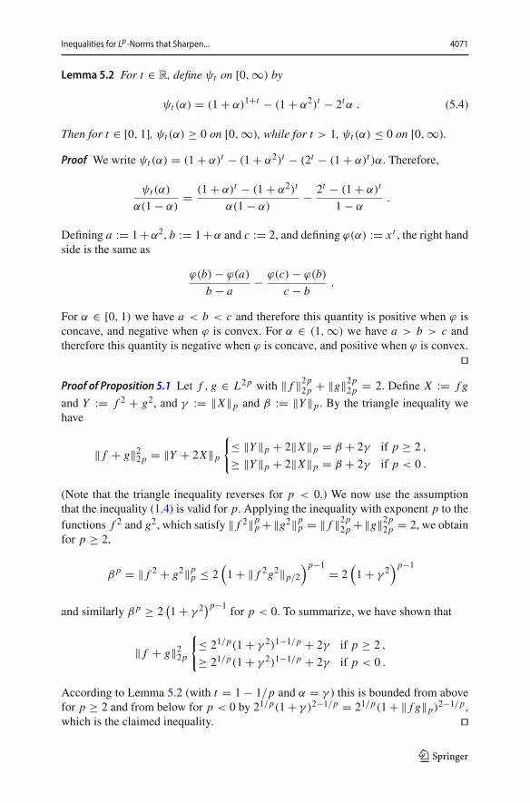
Lemma 5.2 For t ∈ R, define ψt on [0,∞) by

ψt (α) = (1 + α)1+t − (1 + α2)t − 2tα . (5.4)

Then for t ∈ [0, 1], ψt (α) ≥ 0 on [0,∞), while for t > 1, ψt (α) ≤ 0 on [0,∞).

Proof We write ψt (α) = (1 + α)t − (1 + α2)t − (2t − (1 + α)t )α. Therefore,

ψt (α)

α(1 − α)= (1 + α)t − (1 + α2)t

α(1 − α)− 2t − (1 + α)t

1 − α.

Defining a := 1+α2, b := 1+α and c := 2, and defining ϕ(α) := xt , the right handside is the same as

ϕ(b) − ϕ(a)

b − a− ϕ(c) − ϕ(b)

c − b.

For α ∈ [0, 1) we have a < b < c and therefore this quantity is positive when ϕ isconcave, and negative when ϕ is convex. For α ∈ (1,∞) we have a > b > c andtherefore this quantity is negative when ϕ is concave, and positive when ϕ is convex.

�Proof of Proposition 5.1 Let f , g ∈ L2p with ‖ f ‖2p

2p + ‖g‖2p2p = 2. Define X := f g

and Y := f 2 + g2, and γ := ‖X‖p and β := ‖Y‖p. By the triangle inequality wehave

‖ f + g‖22p = ‖Y + 2X‖p

{≤ ‖Y‖p + 2‖X‖p = β + 2γ if p ≥ 2 ,

≥ ‖Y‖p + 2‖X‖p = β + 2γ if p < 0 .

(Note that the triangle inequality reverses for p < 0.) We now use the assumptionthat the inequality (1.4) is valid for p. Applying the inequality with exponent p to thefunctions f 2 and g2, which satisfy ‖ f 2‖p

p +‖g2‖pp = ‖ f ‖2p

2p +‖g‖2p2p = 2, we obtain

for p ≥ 2,

β p = ‖ f 2 + g2‖pp ≤ 2

(1 + ‖ f 2g2‖p/2

)p−1 = 2(1 + γ 2

)p−1

and similarly β p ≥ 2(1 + γ 2

)p−1for p < 0. To summarize, we have shown that

‖ f + g‖22p

{≤ 21/p(1 + γ 2)1−1/p + 2γ if p ≥ 2 ,

≥ 21/p(1 + γ 2)1−1/p + 2γ if p < 0 .

According to Lemma 5.2 (with t = 1 − 1/p and α = γ ) this is bounded from abovefor p ≥ 2 and from below for p < 0 by 21/p(1+ γ )2−1/p = 21/p(1+ ‖ f g‖p)

2−1/p,which is the claimed inequality. �

123


5.2 A Generalization to Schatten Norms

For p ∈ [1,∞), an operator A on some Hilbert space belongs to the Schatten p-class Sp in case (A∗ A)p/2 is trace class, and the Schatten p norm on Sp is definedby ‖A‖p = (Tr[(A∗ A)p/2])1/p. One possible noncommutative analog of (part of)Theorem 1.1 would assert that for positive A, B ∈ Sp, p > 2.

Tr(A + B)p ≤⎛

⎝1 +(Tr[B p/4Ap/2B p/4]12‖A‖p

p + 12‖B‖p

p

)2/p⎞

⎠

p−1

Tr(

Ap + B p ). (5.5)

Note that for p = 2, (5.5) holds as an identity.In this setting, it is not clear how to implement analogs of Parts A and B of our proof

for functions. However, the direct proofs sketched at the beginning of this section doallow us to prove the validity of (5.5) for all p = 2k , k ∈ N.

Theorem 5.3 If (5.5) is valid for some p ≥ 2 and all positive A, B ∈ Sp, then it isvalid for 2p and all A, B ∈ S2p. In particular, since (5.5) holds as an identity forp = 2, it is valid for p = 2k for all k ∈ N.

Proof Let A and B be positive operators in S2p, and assume that ‖A‖2p2p +‖B‖2p

2p = 2,which, by homogeneity, entails no loss of generality. Define

X := 1

2(AB + B A) and Y = A2 + B2 .

Note that

‖X‖p ≤ 1

2(‖AB‖p + ‖B A‖p) .

By definition, the Lieb–Thirring inequality [10], and cyclicity of the trace,

‖AB‖pp = Tr[(B A2B)p/2] ≤ Tr[B p/2Ap B p/2] = Tr[Ap/2B p Ap/2] .

Define

β := ‖Y‖p and γ := (Tr[B p/2Ap B p/2])1/p .

Therefore, ‖A + B‖22p = ‖Y + 2X‖p ≤ ‖Y‖p + 2‖X‖p ≤ β + 2γ . Since ‖A2‖pp +

‖B2‖pp = 2, we can apply (5.5) to deduce that

β p = ‖A2 + B2‖pp ≤ 2

(1 + (Tr[B2p/4Ap B2p/4])2/p

)p−1 = 2(1 + γ 2

)p−1.

Altogether

‖A + B‖22p ≤ 21/p(1 + γ 2)1−1/p + 2γ

123


and, by Lemma 5.2, the right side is bounded above by 21/p(1+γ )2−1/p, which provesthe inequality, �Note Since this paper was submitted, two further papers by the authors [5,8] haveappeared which, in particular, explore extensions of the inequalities discussed here tomore than three functions. The results are less complete than for two functions.

Acknowledgements Open Access funding provided by Projekt DEAL. We thank Anthony Carbery foruseful correspondence.

OpenAccess This article is licensedunder aCreativeCommonsAttribution 4.0 InternationalLicense,whichpermits use, sharing, adaptation, distribution and reproduction in any medium or format, as long as you giveappropriate credit to the original author(s) and the source, provide a link to the Creative Commons licence,and indicate if changes were made. The images or other third party material in this article are includedin the article’s Creative Commons licence, unless indicated otherwise in a credit line to the material. Ifmaterial is not included in the article’s Creative Commons licence and your intended use is not permittedby statutory regulation or exceeds the permitted use, you will need to obtain permission directly from thecopyright holder. To view a copy of this licence, visit http://creativecommons.org/licenses/by/4.0/.

References

1. Clarkson, J.A.: Uniformly convex spaces. Trans. Am. Math. Soc. 40, 396–414 (1936)2. Ball, K., Carlen, E.A., Lieb, E.H.: Sharp uniform convexity and smoothness inequalities for trace

norms. Invent. Math. 115(3), 463–482 (1994)3. Carbery, A.: Almost orthogonality in the Schatten-von Neumann classes. J. Oper. Theory 62(1), 151–

158 (2009)4. Carlen, E.A., Frank, R.L., Lieb, E.H.: Stability estimates for the lowest eigenvalue of a Schrödinger

operator. Geom. Funct. Anal. 24(1), 63–84 (2014)5. Carlen, E.A., Frank, R.L., Lieb, E.H.: Inequalities that sharpen the triangle inequality for sums of N

functions in L p . Ark. Math. 58(1), 57–69 (2020)6. Hanner, O.: On the uniform convexity of L p and p . Ark. Math. 3, 239–244 (1956)7. Hardy, G., Littlewood, J.E., Polya, G.: Inequalities. Cambridge Univ Press, Cambridge (1934)8. Mooney, C., Ivanisvili, P.: Sharpening the triangle inequality: envelopes between L2 and L p spaces.

Anal. PDE (to appear)9. Lieb, E.H., Loss, M.: Analysis, 2nd edn. American Mathematical Society, Providence, RI (2014)

10. Lieb, E.H., Thirring,W.: Inequalities for themoments of the eigenvalues of the Schrödinger hamiltonianand their relation to Sobolev inequalities. In: Lieb, E.H., Simon, B., Wightman, A. (eds.) Studies inMathematical Physics, pp. 269–303. Princeton University Press (1976)

Publisher’s Note Springer Nature remains neutral with regard to jurisdictional claims in published mapsand institutional affiliations.

123

http://creativecommons.org/licenses/by/4.0/

Inequalities for -Norms that Sharpen the Triangle ...

Documents

Transcript of Inequalities for -Norms that Sharpen the Triangle ...