INDE 2333ENGINEERING STATISTICS I

GOODNESS OF FIT

University of HoustonDept. of Industrial Engineering

Houston, TX 77204-4812(713) 743-4195

AGENDA

Chi-square goodness of fit test

GOODNESS OF FIT TESTS

Used to determine if a sample could have come from a distribution with the specified parameters

Commonly used to determine if data is normally distributed Many tests such as the ones that we have been using require normally

distributed data. If data is not normally distributed, non-parametric tests must be used

(next subject in the course) Also used for input distributions in system modeling

Customers or jobs arrive exponentially distributed? Service times follow what distribution? Failures occur according to what distribution?

GOODNESS OF FIT TESTS

Based on a comparison of observations between Observed data Theoretical data

The comparison utilizes a set of intervals or cells Each cell has a lower and upper boundary values The determination of the boundaries are a function of

Theoretical distribution Number of observations in the sample 2 different approaches…

TWO DIFFERENT APPROACHES

Approach 1 Used in the book Equal interval approach No cell grouping can have less than 5 expected observations

Approach 2 Used in other books Equiprobable approach Maximum number of cells not to exceed 100 such that the expected number of

observations is at least 5 = Int ( obs/5 ) Expected number of obs in each cell = obs / cells More statistically robust

HYPOTHESES TEST PROCEDURE

Identify Ho and Ha Determine level of significance (generally 0.05 or 0.01) Determine “critical value” criterion from level of

significance Calculate “test statistic” Make decision

Fail to reject Ho Reject Ho

HYPOTHESES

Ho The sample could have come from a distribution with the

specified parameters Ha

The sample could not have come from a distribution with the specified parameters

CRITICAL VALUE

Chi-square distribution chart One sided test Alpha typically 0.05 Degrees of freedom

# of cells - # of parameters used from sample -1 The -1 is always used due to the known sample size n Note, if the parameters are specified not sampled then they do not

reduce the number of degrees of freedom in the above equation

CHI-SQUAREfor a particular number of degrees of freedom

f(X^2)

X^20 X^2 Critical value

Right tail probability, alpha, typically 0.05

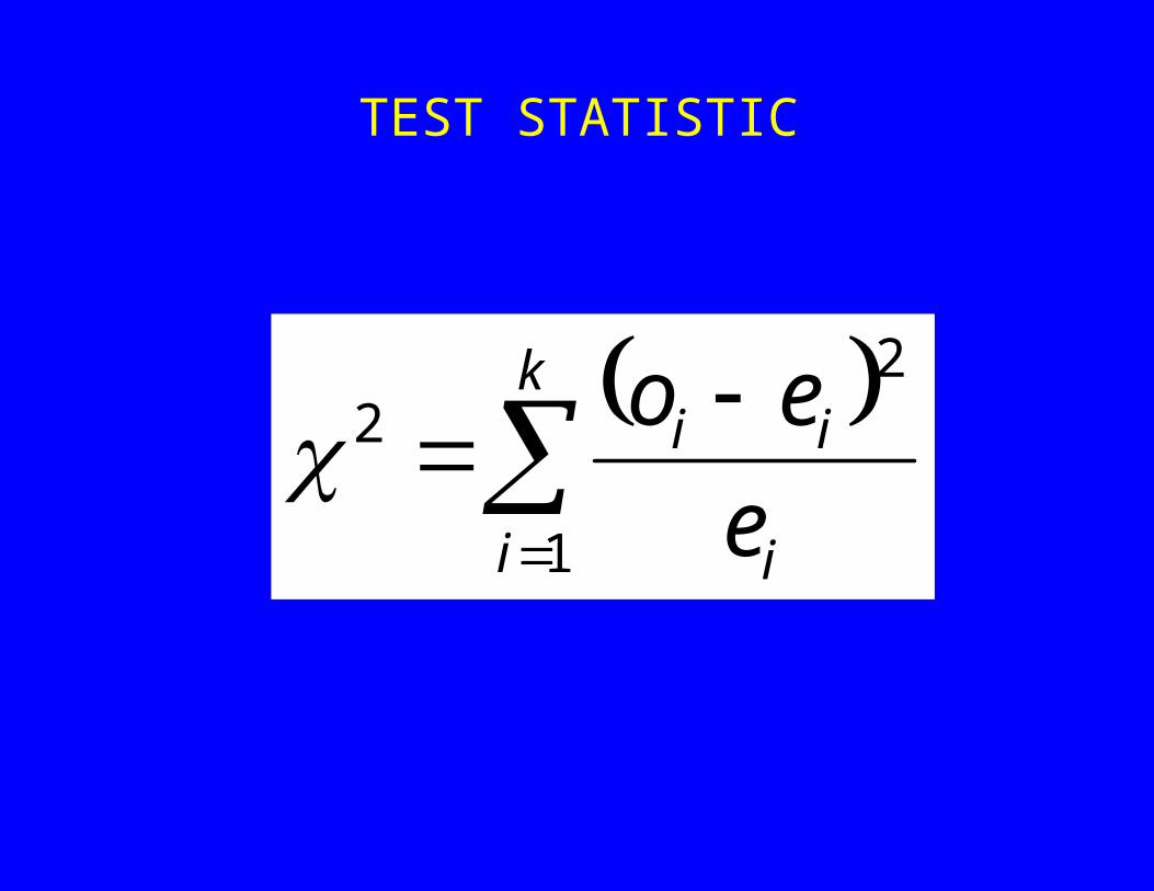
TEST STATISTIC

k

i i

ii

e

eo

1

22

DECISION

Cannot reject Test statistic is less than the critical value Sample could have come from a distribution with the

specified parameters Reject

Test statistic is greater than the critical value Sample could not have come from a distribution with the

specified parameters

EXAMPLE 1EQUAL INTERVAL APPROACH

400 5 minute intervals were observed for air traffic control messages

At alpha=0.01, is the distribution of the number of messages able to be considered as having a poisson distribution with a mean of 4.6?

Approach Lamba parameter of 4.6 is given Use the poisson table probability table for 4.6 Multiply the probability by 400 to obtain the expected observations Compare the actual observations to the expected observations

HYPOTHESES

Ho: Poisson distribution with mean of 4.6

Ha: Not poisson distribution with a mean of 4.6

Messages Observed Probability Expected

0 3 Combine 0.010 4.0 Combine

1 15 for 18 0.046 18.4 For 22.4

2 47 0.107 42.8

3 76 0.163 65.2

4 68 0.187 74.8

5 74 0.173 69.2

6 46 0.132 52.8

7 39 0.087 34.8

8 15 0.050 20.0

9 9 0.025 10.0

10 5 Combine 0.012 4.8 Combine

11 2 these 4 0.005 2.0 These 4

12 0 cells for a 0.002 0.8 Cells for a

13 1 total of 8 0.001 0.4 total of 8

CHI-SQUAREfor 10-1 degrees of freedom

f(X^2)

X^20 16.919 Critical value

Right tail probability, alpha = 0.01

TEST STATISTIC

749.68

88...

8.42

8.4247

4.22

4.2218 2222

DECISION

Test statistic of 6.749 is less than the critical value of 16.919

Cannot reject Ho of distribution being poisson with a mean of 4.6

There is evidence to support the claim that the data came from a poisson distribution with a mean of 4.6 at an alpha level of 0.01

EXAMPLE 2EQUIPROBABLE APPROACH

Were the scores from an INDE 2333 exam normally distributed?

Sample statistics Mean=71.95 Std=11.93 N=43

HYPOTHESES

Ho The sample could have come from a normally distributed

population with a mean of 71.95 and a std of 11.93 Ha

The sample could not have come from a normally distributed population with a mean of 71.95 and a std of 11.93

CRITICAL VALUE

Chi-square distribution chart One sided test 0.05 Degrees of freedom

The sample size is 43 Want the maximum number of cells not to exceed 100 with a minimum

expected number of observation of 5 43/5=8.6 cells With 8 cells, the expected number of observations is 5.375 Degrees of freedom is number of cells – number of parameters used from

sample-1 Degrees of freedom=8-2-1=5

CHI-SQUAREfor 5 of degrees of freedom

f(X^2)

X^20 11.070

0.05

TEST STATISTIC

k

i i

ii

e

eo

1

22

CELL BOUNDARIES

To calculate observed values in each cell, we must determine the actual x cell boundaries from the 8 equiprobable cells

For normal distributions Look up z value corresponding to probability Boundaries =mean+std * Z

CALCULATING OBSERVATIONS

Cell Lower% Upper% Lower

Z

Upper

Z

lowerx upperx obs exp

1 0 0.125 -inf 0 58.227 5 5.375

2 0.125 0.250 58.227 63.905 6 5.375

3 0.250 0.375 63.905 68.151 5 5.375

4 0.375 0.500 0 68.151 71.953 3 5.375

5 0.500 0.625 0 71.953 75.756 5 5.375

6 0.625 0.750 75.756 80.002 5 5.375

7 0.750 0.875 80.002 85.680 5 5.375

8 0.875 1.000 +inf 85.680 100.00 8 5.375

CALCULATING TEST STATISTIC

Cell obs exp ((O-E)^2)/E

1 5 5.375 0.026

2 6 5.375 0.072

3 5 5.375 0.026

4 3 5.375 1.049

5 5 5.375 0.026

6 5 5.375 0.026

7 5 5.375 0.026

8 8 5.375 1.282

Total 2.534

DECISION

2.581 < 11.070 Cannot reject the Ho Evidence to support the claim that the test scores are

normally distributed with a mean of 71.95 and std of 11.93

IN EXCEL

Frequency Data_array, bins_array

Range operation CTRL-SHIFT-ENTER

Norminv function Probability, mean, std

Chiinv function Probability, df