Income Eﬀects of Time Allocation in Poor South African ... · PDF fileIncome Eﬀects of...

Income Effects of Time Allocation in Poor South

African Households: Evidence from South Africa’s Old

Age Pension

Vimal Ranchhod ∗

Martin Wittenberg †

May 8, 2007

Abstract

How do poor households in developing countries change their time allocation in

response to an anticipated increase in income. Using the age-eligibility of the South

African Old Age Pension for identification, we inform this question using South African

time use data. We find that time allocation to productive consumption, home produc-

tion, market work, and leisure all change amongst non-recipients in the household.

The magnitudes, significance and dimensions of reallocation differs by the gender of

the household member. Women reduce their time in both home production and market

production. Men do too, but the coefficients are generally smaller and are seldom sig-

nificant. Both genders seem to increase their time spent in leisure activities, but again,

it seems the females are more sensitive. Men, however, significantly increase the time

they spend eating. Policy evaluations that fail to account for these intra-household

∗PhD Candidate, Dept. of Economics, University of Michigan. Email: [email protected]†Assoc. Prof., Dept. of Economics, University of Cape Town. Email: [email protected]

adjustments of time allocation are likely to provide an incomplete assessment of the

effects of these cash transfers.

PRELIMINARY AND INCOMPLETE. PLEASE DO NOT CITE.

Comments and suggestions are most welcome.

2

1 Introduction

How do prime aged household members in developing countries respond to an exogenous

increase in non-market income? In particular, how does it affect their choices regarding time

allocation to various activities? We explore this question using nationally representative

time use data from South Africa. We make use of the age of resident elderly members, in

conjunction with pension eligibility rules to identify the aforementioned income effects.

Time is one of the most valuable resources available to individuals and families. Through

employment and wages, the financial budget constraint and time budget constraints are

clearly related. Thus, a relaxing of the household’s financial constraints is likely to affect the

goods purchased by the household, the quantity and types of home production activities, as

well as the consumption of leisure by various household members.

Several researchers have explored the relationship between income transfers and various mea-

sures of social and economic well being. These include poverty, nutrition and health, adult

labor, child labor, schooling enrollment, intra-household bargaining outcomes and pooling

of resources across households. In the South African context, effects on time allocation have

been restricted to crude measures of schooling enrollment and labor force participation. To

date, the impact on specific time allocation choices in recipient households has been ignored.

Given that households do indeed share resources, and that multi-generational households

are common, we obtain an incomplete understanding of the impacts of such policies if our

analyses excludes the impacts on time allocation.

Policy implications notwithstanding, simply knowing the responsiveness of people’s time

with respect to income is an economically interesting query. Revealed preferences suggests

that any observed changes will reflect the optimal allocation of the income transfer to a new

set of time allocation and consumption bundles. Observing these allows us to gauge some

element of household preferences, even if not very cleanly.

In this paper, we use data from the South African Time Use Survey of 2000. This is a

3

large, nationally representative dataset which reports respondents’ activities the previous

day, as well as a household roster with each member’s demographic information. Included

in the household roster are basic income and welfare measures. To identify income effects,

we make use of the the age eligibility rules that govern the South African Old Age Pension

(OAP). The OAP is a relatively generous means tested income transfer, which is universally

available, non-contributory and highly anticipated. Our investigation in essence involves the

comparison of the time allocation of prime aged adults who live with an elderly person who

is not yet of pensionable age, with similar individuals who live with an elderly person who

is pension age-eligible.

Our analysis consists of two methods. We first perform non-parametric analyses and present

the results graphically. While these are less constrained by the structure imposed by a

specification in a regression, they are also less informative in some ways. We then employ

multivariate regression techniques to estimate parametric models which allow us to control

for additional differences between the two groups. In a nutshell, we observe that adults in the

household respond in several dimensions of time allocation, including market work, informal

sector services, child care, time spent eating, sleeping and socializing.

2 Literature and Pension Rules

Related Pension Literature

Several researchers have investigated the effects of pension recipiency on various dimensions

of household welfare. Case and Deaton (1998) analyze the redistributive consequences of

the OAP, and find that the OAP is an effective transfer to the poor and poverty stricken in

general. Duflo (2000), Case (2001), and Duflo (2003) all find that the health of household

members is improved as a result of the pension.

Jensen (2003) estimates that crowding out of remittances by pensions is large and significant.

4

On average, every rand of pension income received by the elderly is met with a 0.25 to 0.30

rand decrease in remittances received from the pensioner’s children. Pension income is thus

de facto shared with non-resident family members as well.

Most recently, Edmonds et al (2005) find that household composition itself is affected by

someone becoming pension age-eligible. They find a decrease in the number of prime working-

age women, and an increase in the number of children younger than five and young women

of childbearing age.

Bertrand et al (2003) find that having a pension eligible person in the household has a

statistically significant and negative impact on the labor supply of prime aged individuals in

the household. Edmonds (2003) finds that when a household member who is male becomes

pension eligible, there is a sizable decline in child labor, coupled with an increase in schooling

attendance and attainment. Ranchhod (2006) finds that the pension induces sharp levels of

labor force withdrawal amongst the elderly themselves.

All of these suggest that we might reasonably expect that the pension may cause changes in

the time allocation of adult household members as well. Estimating these income effects is

the primary contribution of this paper.

Pension Rules

Lund (1993) provides an introduction to the OAP as we see it today. As stated previously,

the pension is means tested, and provides a relatively generous cash transfer to recipients.

Eligibility depends only on age, nationality and satisfying the means test. The age-eligibility

threshold is 60 for women and 65 for men. The level of the means test is set fairly high,

so that most of the elderly receive the grant. 1 Ranchhod (2006) notes that the prevailing

distribution of observed wages amongst the elderly is such that most of the elderly could

1Data from the September wave of the South African Labour Force Survey indicates that about 80% of

age-eligible African South Africans report receiving the pension.

5

continue to work while still satisfying the requirements to receive the pension.

Moreover, the means test is based on individual income for the unmarried elderly, or joint

spousal income for married couples. Hence, it should not have direct distortionary ‘implicit

taxation’ effects for other non-elderly household members, although it implicitly does change

the costs of market time for some pensioners and thus for some households.

The value of the pension is adjusted periodically, usually on an annual basis, to adjust for

inflation. In 2000, the period during which our data was collected, this was 540 South African

rands per month. Depending on the exchange rate and inflation rate, this generally equates

to between 100 and 125 US dollars per month in current terms. 2 This is a large transfer

relative to potential wage income, and continues for as long as the pensioner remains alive

and continues to satisfy the means test.

3 Theory

We adopt the model provided by Becker in his seminal paper on “A Theory of the Allocation

of Time” (1965). In this model, the household acts to maximize utility by consuming a

bundle of commodities Z, subject to an income constraint, a time constraint, and constraints

imposed by the technology of production.3 Formally, the household’s optimization problem

is written as:

max U(Z1, . . . , Zm) (1)

subject to :

Zi = fi(xi, Ti) (2)

2Own Calculations. The deflator used is the official Consumer Price Index released by Statistics South

Africa.3While a unitary household preference seems unreasonable given the existing empirical findings on the

OAP, we are not attempting to test between the competing models of intra-household allocation of resources.

As such, the unitary model suffices for providing a relatively simple framework within which we can interpret

our findings.

6

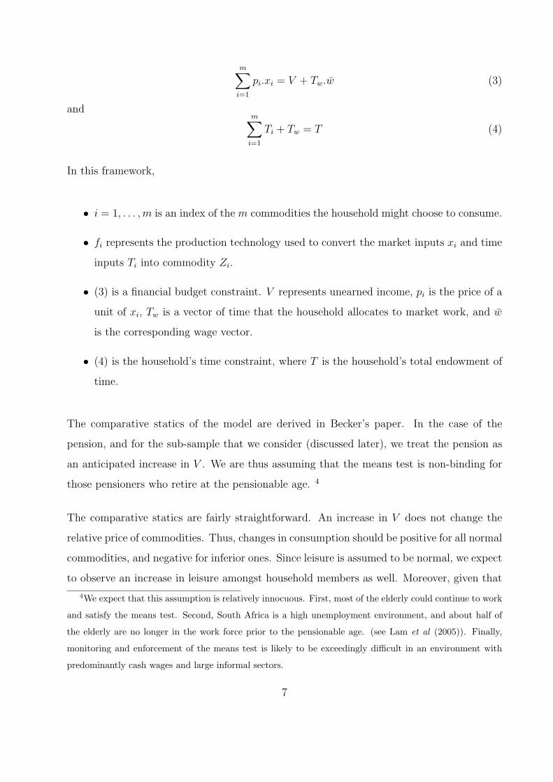
m∑i=1

pi.xi = V + Tw.w̄ (3)

andm∑

i=1

Ti + Tw = T (4)

In this framework,

• i = 1, . . . ,m is an index of the m commodities the household might choose to consume.

• fi represents the production technology used to convert the market inputs xi and time

inputs Ti into commodity Zi.

• (3) is a financial budget constraint. V represents unearned income, pi is the price of a

unit of xi, Tw is a vector of time that the household allocates to market work, and w̄

is the corresponding wage vector.

• (4) is the household’s time constraint, where T is the household’s total endowment of

time.

The comparative statics of the model are derived in Becker’s paper. In the case of the

pension, and for the sub-sample that we consider (discussed later), we treat the pension as

an anticipated increase in V . We are thus assuming that the means test is non-binding for

those pensioners who retire at the pensionable age. 4

The comparative statics are fairly straightforward. An increase in V does not change the

relative price of commodities. Thus, changes in consumption should be positive for all normal

commodities, and negative for inferior ones. Since leisure is assumed to be normal, we expect

to observe an increase in leisure amongst household members as well. Moreover, given that

4We expect that this assumption is relatively innocuous. First, most of the elderly could continue to work

and satisfy the means test. Second, South Africa is a high unemployment environment, and about half of

the elderly are no longer in the work force prior to the pensionable age. (see Lam et al (2005)). Finally,

monitoring and enforcement of the means test is likely to be exceedingly difficult in an environment with

predominantly cash wages and large informal sectors.

7

a significant number of the elderly retire when they become eligible for the pension, the

household potentially gets a large increase in adult time for home production activities.

This is likely to further affect adult members’ time allocation behaviors, as the pension is

then also implicitly relaxing the non-elderly adults’ time constraints.

4 Data

Sampling methodology

The South African Time Use Survey was carried out by Statistics South Africa in 2000. The

information is based on recall diaries from about 14 000 individuals. The individuals were

selected in a three stage sampling process. In the first stage 902 primary sampling unit were

selected from a set of enumerator areas stratified by location, viz. urban formal, urban infor-

mal, commercial farming and ex-homeland rural areas. The urban informal and commercial

farming areas were oversampled at this stage. In the second stage dwellings were sampled

within these clusters and in the third two individuals (if the household had two or more

eligible individuals, otherwise one individual) were selected based on a randomization proce-

dure within the household. Only individuals aged ten above were eligible to be interviewed.

Statistics South Africa have provided a set of weights to correct for the different sampling

probabilities. These weights are used in all the estimation procedures reported below.

In order to account for some seasonal and weekly variations in time use, the survey was

collected in three tranches: February, June and October. Within each tranche attempts were

made to collect information across the working week. Unlike with some surveys conducted

in other countries, however, no attempt was made to interview the same individual on more

than one day. This means that we cannot investigate any day-to-day variation in the choices

made (e.g. in relation to home work).

The information was recorded through three different instruments. Once the household had

8

been selected a household level questionnaire was administered to a knowledgeable person.

This questionnaire included some basic socio-economic information on the entire household,

such as access to services and total household income. A roster of household members

provided the basis from which to select the individuals to be interviewed further. The

selected individuals were asked a set of questions about themselves, such as educational

attainment, marital status, labour market participation and personal income. The main

focus of the personal interviews, however, was the time diary.

Measuring time allocation

Individuals were interviewed about their use of time during the previous twenty-four hours.

The activities were recorded within half-hour time slots according to an ”activity classi-

fication system”. Frequently reported categories included ’sleep’, various forms of ‘work’,

‘cooking’, ‘cleaning’, ‘watching TV’, ‘listening to the radio’, various forms of ‘socializing’

,‘childcare’ and ‘doing nothing’. Provision was made for up to three activities in each slot.

In order to convert slots into actual time use, we simply divided the thirty minutes between

the activities recorded in that time.

One of the questions that arises with a recall diary in the South African context is whether

the informants, many of whom do not own watches, are able to give sufficiently accurate

information about what happened in particular time slots. The problem is not only forget-

ting, but the ability to anchor activities to times of the day. Some exploratory work done by

Statistics South Africa suggests that there are many ways in which even rural South Africans

succeed in doing so . They use radio and TV schedules, the passage of buses and trains and

information from other individuals to keep track of time.

9

Sample Selection

Our investigation focusses on the changes in activities amongst adult African South Africans.

We additionally pay specific attention to ‘prime aged’ adults, who we categorized as adults

aged 25 to 55 inclusive. The race restriction was imposed in order to keep our study compa-

rable to the existing OAP literature. It is also beneficial because our proxy for the pension

is age, and a majority of age-eligible Africans receive the pension. 5 In our regressions, we

also restricted the sample to respondents who reported weekday activities. This was done

as minutes spent working was of particular interest to us. 6

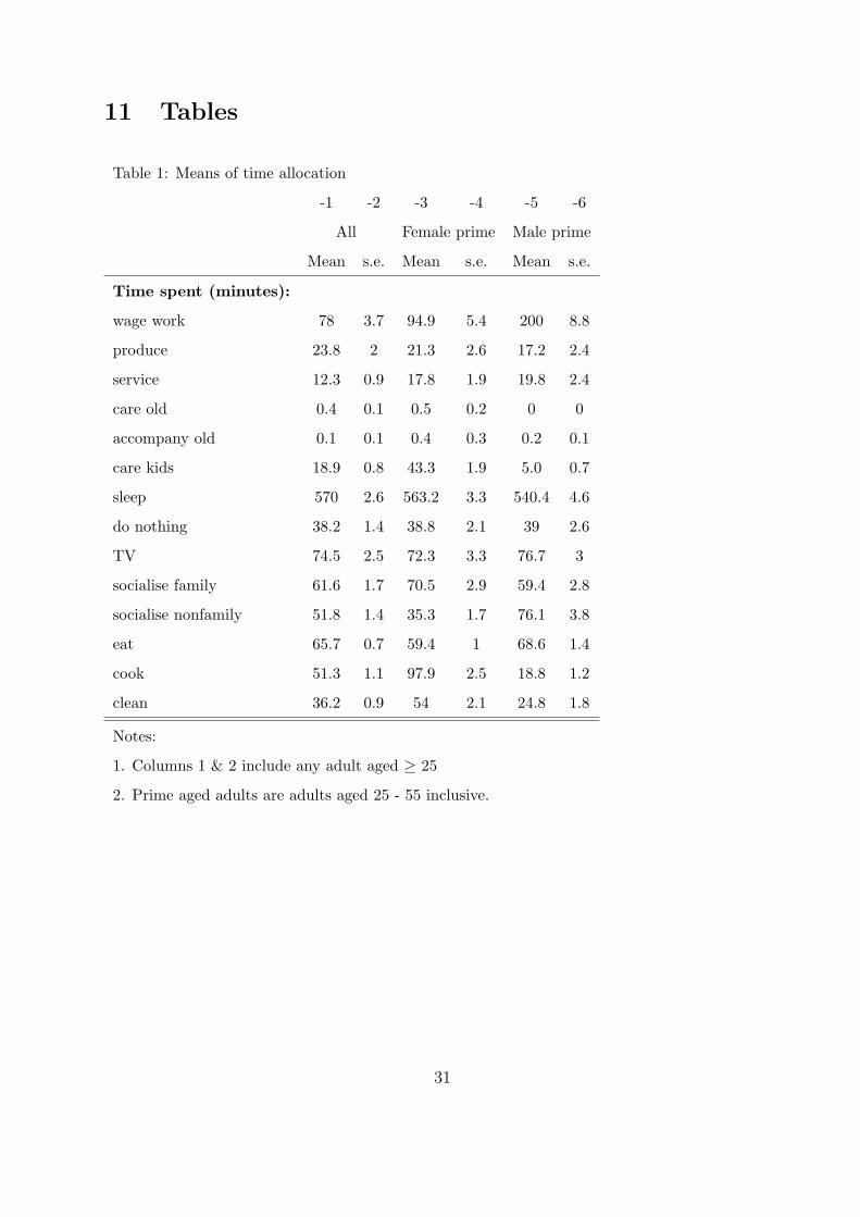
Table 1 shows the mean minutes and standard errors spent in various categories across the

three different regression samples. The largest expenditure of time is spent in sleeping. This

is followed by home production for women and wage related employment for men. Various

forms of socializing, including ‘doing nothing’, takes up between 3.5 and 4 hours on an

average weekday.

Table 2 shows the mean values of the various covariates included in the regressions. Slightly

fewer than half of the respondents are male. The mean years of schooling is between 7.5

and 8.6 years, depending on the sample being considered. Amongst the prime aged adults,

almost one in five women and one in four men have some post high school education. Slightly

more than 15% of prime aged males and females co-reside with a pensioner.

5 Empirical Strategy

Our investigation composes of two methods of analysis. First, we make use of non-parametric

techniques to describe the changes observed between households where the eldest resident

is pension age-eligible and those where said resident is not. These are informative both to

5The proportion of age-eligible white South Africans who receive the OAP is approximately 30% in the

September 2000 Labour Force Survey.6In our non-parametric estimates, we included weekend observations to increase the density of our data.

10

obtain a feel for the data as well as to visually observe that some adjustments do seem to

occur in anticipation of the pension. Our sample in this case is the pooled set of prime aged

African males and females. We employ locally weighted regressions with a bandwidth of

0.3 and 0.5 for non-pensioner and pensioner households respectively. The set of dependent

variables are the time allocation of respondents to various activities, and to the extent that

the data allows, ownership of relevant consumer durables such as radios, TVs and cars.

Second, we perform regression analyses on some of the time allocation variables. This allows

us to obtain numerical estimates of the effect of having a pensioner present, with corre-

sponding standard errors. We control for the individual demographic characteristics of the

respondents, such as their age and education, as well as their geographic and household

composition attributes. We estimate each regression for both genders combined, as well

as separately for men and women. Our estimation samples include all adults, prime aged

women and prime aged men.

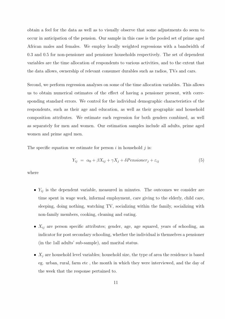
The specific equation we estimate for person i in household j is:

Yij = α0 + βXij + γXj + δPensionerj + εij (5)

where

• Yij is the dependent variable, measured in minutes. The outcomes we consider are

time spent in wage work, informal employment, care giving to the elderly, child care,

sleeping, doing nothing, watching TV, socializing within the family, socializing with

non-family members, cooking, cleaning and eating.

• Xij are person specific attributes; gender, age, age squared, years of schooling, an

indicator for post secondary schooling, whether the individual is themselves a pensioner

(in the 1all adults’ sub-sample), and marital status.

• Xj are household level variables; household size, the type of area the residence is based

eg. urban, rural, farm etc , the month in which they were interviewed, and the day of

the week that the response pertained to.

11

• Our primary coefficient of interest is δ. Pensionerj is an indicator variable that takes

on a value of one if there is at least one pensioner in the household. Thus δ provides

us with the mean difference in time allocation between the group of respondents who

reside with a pensioner and those who do not.

In all cases, robust standard errors were estimated and clustered at the household level.

6 Results

Non-parametric results

The non-parametric regression results are presented graphically in Figures 1 through 23.

Since the pensionable age is 65 for men, there are some respondents who live with someone

aged above 60 who do not live with a pensioner. Given that these are simply bivariate

regressions, we interpret them with caution. However, the ‘gap’ observed in some cases

are valid estimators of the effect of the pension insofar as the effects of the pension can be

interpreted in a regression discontinuity framework. The dependent variables can be grouped

within the broadly defined categories of market activities, home production, productive

consumption and leisure. We also estimate asset ownership where possible.

In the productive consumption group (Fig. 1-2), we find a big increase in time spent eating,

of about 10 minutes. This represents an increase of more than 15%. We do not observe a

clear change in time spent on religious activities.

In the leisure activities group (Fig. 3-9), we observe some increase in the minutes spent doing

‘nothing’, and an increase in time spent socializing with both family as well as non-family

members. The increase in socializing within families is about 20 minutes, an increase of

more than 30%. Sleep, radio listening and TV watching do not seem to be discontinuously

affected, although TV watching does occur at a higher level amongst those who live with a

12

pensioner. 7

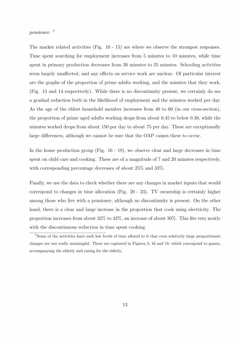
The market related activities (Fig. 10 - 15) are where we observe the strongest responses.

Time spent searching for employment increases from 5 minutes to 10 minutes, while time

spent in primary production decreases from 30 minutes to 25 minutes. Schooling activities

seem largely unaffected, and any effects on service work are unclear. Of particular interest

are the graphs of the proportion of prime adults working, and the minutes that they work,

(Fig. 13 and 14 respectively). While there is no discontinuity present, we certainly do see

a gradual reduction both in the likelihood of employment and the minutes worked per day.

As the age of the eldest household member increases from 40 to 60 (in our cross-section),

the proportion of prime aged adults working drops from about 0.45 to below 0.30, while the

minutes worked drops from about 150 per day to about 75 per day. These are exceptionally

large differences, although we cannot be sure that the OAP causes these to occur.

In the home production group (Fig. 16 - 19), we observe clear and large decreases in time

spent on child care and cooking. These are of a magnitude of 7 and 20 minutes respectively,

with corresponding percentage decreases of about 25% and 33%.

Finally, we use the data to check whether there are any changes in market inputs that would

correspond to changes in time allocation (Fig. 20 - 23). TV ownership is certainly higher

among those who live with a pensioner, although no discontinuity is present. On the other

hand, there is a clear and large increase in the proportion that cook using electricity. The

proportion increases from about 32% to 42%, an increase of about 30%. This fits very neatly

with the discontinuous reduction in time spent cooking.

7Some of the activities have such low levels of time alloted to it that even relatively large proportionate

changes are not really meaningful. These are captured in Figures 3, 16 and 18, which correspond to games,

accompanying the elderly and caring for the elderly.

13

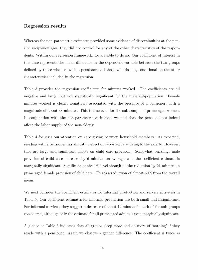
Regression results

Whereas the non-parametric estimates provided some evidence of discontinuities at the pen-

sion recipiency ages, they did not control for any of the other characteristics of the respon-

dents. Within our regression framework, we are able to do so. Our coefficient of interest in

this case represents the mean difference in the dependent variable between the two groups

defined by those who live with a pensioner and those who do not, conditional on the other

characteristics included in the regression.

Table 3 provides the regression coefficients for minutes worked. The coefficients are all

negative and large, but not statistically significant for the male subpopulation. Female

minutes worked is clearly negatively associated with the presence of a pensioner, with a

magnitude of about 38 minutes. This is true even for the sub-sample of prime aged women.

In conjunction with the non-parametric estimates, we find that the pension does indeed

affect the labor supply of the non-elderly.

Table 4 focusses our attention on care giving between household members. As expected,

residing with a pensioner has almost no effect on reported care giving to the elderly. However,

thee are large and significant effects on child care provision. Somewhat puzzling, male

provision of child care increases by 6 minutes on average, and the coefficient estimate is

marginally significant. Significant at the 1% level though, is the reduction by 21 minutes in

prime aged female provision of child care. This is a reduction of almost 50% from the overall

mean.

We next consider the coefficient estimates for informal production and service activities in

Table 5. Our coefficient estimates for informal production are both small and insignificant.

For informal services, they suggest a decrease of about 12 minutes in each of the sub-groups

considered, although only the estimate for all prime aged adults is even marginally significant.

A glance at Table 6 indicates that all groups sleep more and do more of ‘nothing’ if they

reside with a pensioner. Again we observe a gender difference. The coefficient is twice as

14

large for women in both sleep and ‘doing nothing’ (19.53 vs. 8.336 and 18.265 vs 7.869

respectively) and the female coefficient on doing nothing is significant at the 10% level.

In Table 7 our dependent variables are time spent socializing with family members and

non-family members. While pensioners themselves are more likely to socialize outside of

the household, the effect for non-pensioners is not significant. Within the family, however,

socializing certainly becomes more prevalent, with a mean increase of between 11 and 13

minutes.

When we consider time spent on home production of cooking and cleaning, reported in Table

8, we find relatively small coefficient estimates. For prime aged women, the estimates are

not that small, at 10.15 and 9.259 minutes each, but the standard errors are also large and

we cannot claim that they are significant.

In Table 9, our dependent variables are time spent watching TV and Eating. Effects on

TV watching are small and insignificant, while the effects on eating time are sizable and

significant. For prime aged men in particular, we observe an increase in time spent eating of

10 minutes which is significant at the 5% level. Given prior studies on the nutritional effects

of the pension, it is likely that this is brought about by an increase in the purchase of food.

7 Caveats

There are various challenges to our identification strategy. First, there exists significant

measurement error in terms of ages reported due to the ‘age-heaping’ phenomena. Since

respondents tend to heap to numbers ending in ‘zero’ or ‘five’, this becomes particularly

problematic. We believe that this biases us away from finding significant results, and our

estimates are thus conservative.

Second, the pension is fully anticipated. As such, households would optimally smooth their

consumption and time allocations, and we would observe no sharp changes in behavior. Such

15

smoothing will not occur if households are liquidity constrained or highly risk averse. The

non-parametric analysis indicated that there is indeed some pre-pension adjust occurring,

and again we believe our estimates to be conservative.

Third, South Africa has no anti-age discrimination bill. Indeed, compulsory retirement ages

are acceptable as long as they have a long standing precedent within the company. These

ages generally fall at either age 60 or 65. This could be particularly problematic since,

if widespread, our analysis is confounded because the household is obliged to allocate the

pensioner’s time to leisure and home production activities. Our results would not then

be reflecting only the effect of the OAP. This is partially mitigated by the fact that self-

reported retirement rates as well as the willingness to take up an “acceptable offer” exhibit

sharp discontinuities at the pensionable ages for the respective genders. Moreover, relatively

few of the African elderly are employed in formal sector, and the proportion that receive any

form of employer related pension is tiny. (see Ranchhod (2006)).

A final challenge arises if household composition is itself a function of the pension. Some

evidence exists that suggests that this is indeed the case (see Edmonds et al (2005)). De-

pending on the magnitude of such cross-household migration, we need to qualify our findings

to represent not necessarily changes in individuals’ time allocation, but changes in the time

allocation of resident household members.

8 Conclusion

We began this research by asking what income effects the cash transfer that the OAP involves

has on the time allocation of adult household members. Using the nationally representative

time use data from South Africa, and the pension rules for identification, we observed a

number of shifts in the time allocation of prime aged residents.

Combining the findings from our two methodologies, and providing a brief summation, what

have we learnt? In terms of productive consumption, South Africans and particularly males

16

spend significantly more time eating when they live with a pensioner. We observe large

decreases in time worked for both genders amongst prime aged adults, but these results are

larger and significant for prime aged females only. Our non-parametric results also indicated

that prime aged adults smooth their transition out of the labor force in anticipation of the

pension. Prime aged females also spend 50% less time on child care when they live with a

pensioner. This is probably not surprizing since home production is likely to have flexible

hours and females perform most of the home production activities in our data. Leisure is

also consumed in greater quantities by household members. This is manifest in terms of

sleeping, ‘doing nothing’ and socializing. We find almost no time being spent on care giving

to the elderly.

From a policy perspective, this implies that the OAP impacts on the household and its

members in multiple ways. Adults, including the non-elderly, eat more, consume more leisure

and work less, both at home and in the market. While this may or may not be desirable

depending on the social welfare function, it is clear that such cash transfers impact on the

household not only financially, but also in terms of its optimal allocation of time. Policy

evaluations that ignores such time allocation considerations within households are likely to

be inaccurate.

9 References

Becker GS, “A Theory of the Allocation of Time”, Economic Journal 75 (299): 493-517 1965

Case A, “Does money protect health status? Evidence from South African pensions”, NBER

working paper 8495, October 2001

Case A & Deaton A, “Large cash transfers to the elderly in South Africa”, Economic Journal

108 (450): 1330-1361, Sep 1998

Bertrand M, Mullainathan S & Miller D, “Public policy and extended families: Evidence

17

from pensions in South Africa”, World Bank Economic Review 17 (1): 27-50 2003

Duflo E, “Grandmothers and granddaughters: Old-age pensions and intrahousehold alloca-

tion in South Africa”, World Bank Economic Review 17 (1): 1-25 2003

Duflo E, “Child health and household resources in South Africa: Evidence from the Old Age

Pension program”, American Economic Review 90 (2): 393-398 MAY 2000

Edmonds EV, Mammen K & Miller DL, “Rearranging the family? Income support and

elderly living arrangements in a low-income country”, Journal of Human Resources 40 (1):

186-207 WIN 2005

Edmonds EV, “Child labor and schooling responses to anticipated income in South Africa”,

forthcoming in Journal of Development Economics, accepted May 2005

Jensen RT, “Do private transfers ’displace’ the benefits of public transfers? Evidence from

South Africa”, Journal of Public Economics 88 (1-2): 89-112 Jan 2004

Lam D, Leibbrandt M and Ranchhod V, “Labour Force Withdrawal of the Elderly in South

Africa”, CSSR working paper # 118, 2005

Lund, F, . “State social benefits in South Africa.”, International Social Security Review, 46

1993

Ranchhod V, “The effect of the South African old age pension on labour supply of the

elderly”, South African Journal of Economics 74 (4): 725-744 Dec 2006

10 Graphs

18

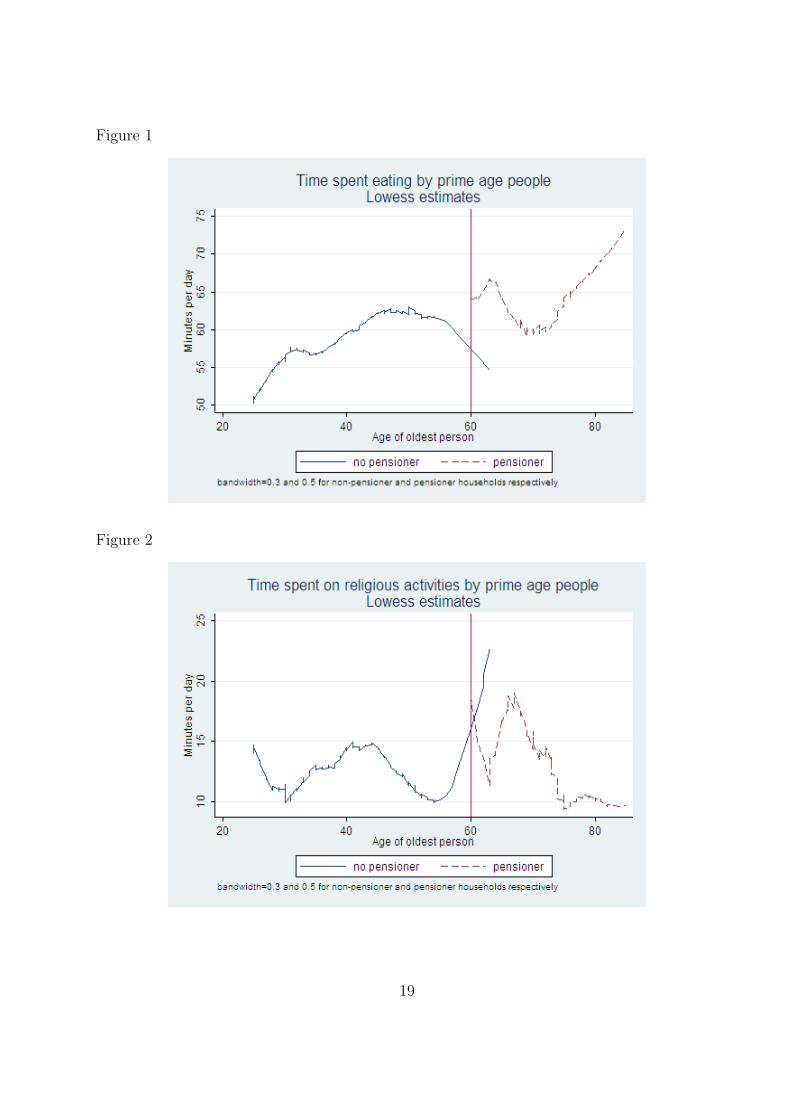
Figure 1

Figure 2

19

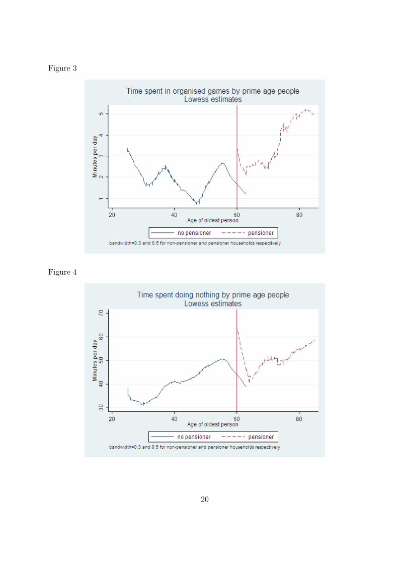
Figure 3

Figure 4

20

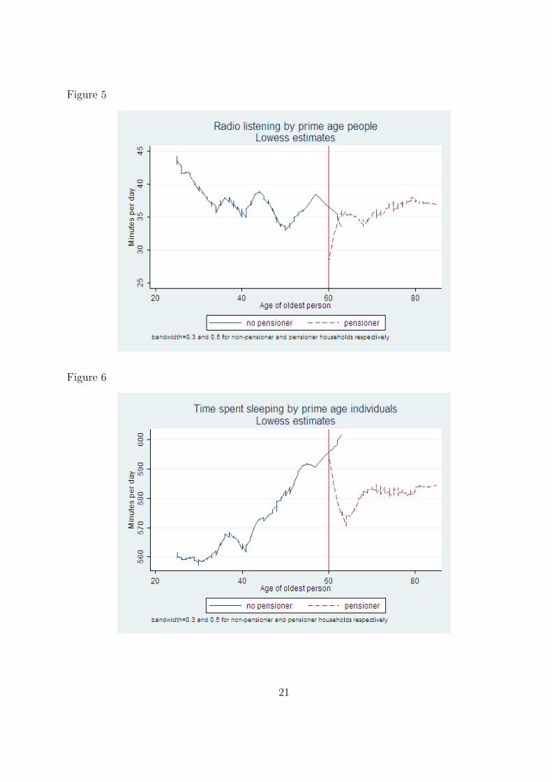
Figure 5

Figure 6

21

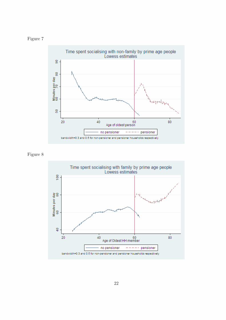
Figure 7

Figure 8

22

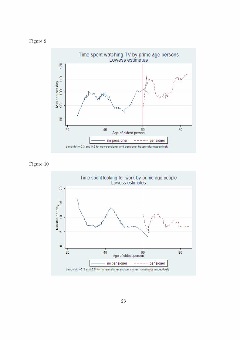
Figure 9

Figure 10

23

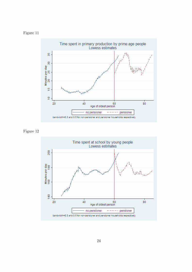
Figure 11

Figure 12

24

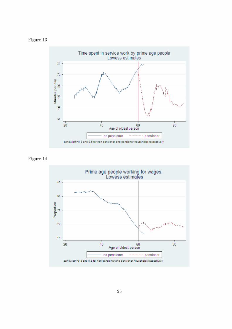
Figure 13

Figure 14

25

Figure 15

Figure 16

26

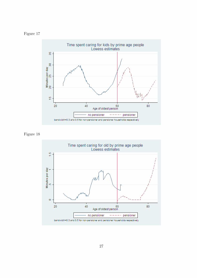
Figure 17

Figure 18

27

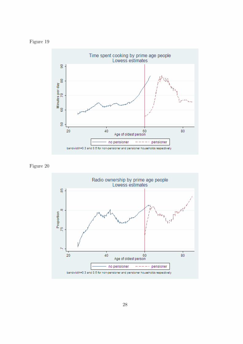
Figure 19

Figure 20

28

Figure 21

Figure 22

29

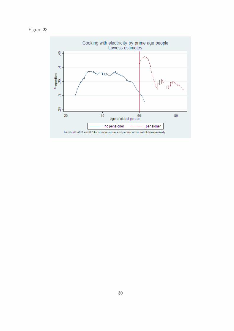
Figure 23

30

11 Tables

Table 1: Means of time allocation

-1 -2 -3 -4 -5 -6

All Female prime Male prime

Mean s.e. Mean s.e. Mean s.e.

Time spent (minutes):

wage work 78 3.7 94.9 5.4 200 8.8

produce 23.8 2 21.3 2.6 17.2 2.4

service 12.3 0.9 17.8 1.9 19.8 2.4

care old 0.4 0.1 0.5 0.2 0 0

accompany old 0.1 0.1 0.4 0.3 0.2 0.1

care kids 18.9 0.8 43.3 1.9 5.0 0.7

sleep 570 2.6 563.2 3.3 540.4 4.6

do nothing 38.2 1.4 38.8 2.1 39 2.6

TV 74.5 2.5 72.3 3.3 76.7 3

socialise family 61.6 1.7 70.5 2.9 59.4 2.8

socialise nonfamily 51.8 1.4 35.3 1.7 76.1 3.8

eat 65.7 0.7 59.4 1 68.6 1.4

cook 51.3 1.1 97.9 2.5 18.8 1.2

clean 36.2 0.9 54 2.1 24.8 1.8

Notes:

1. Columns 1 & 2 include any adult aged ≥ 25

2. Prime aged adults are adults aged 25 - 55 inclusive.

31

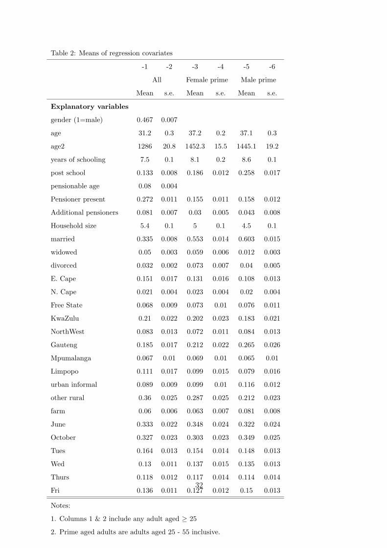
Table 2: Means of regression covariates

-1 -2 -3 -4 -5 -6

All Female prime Male prime

Mean s.e. Mean s.e. Mean s.e.

Explanatory variables

gender (1=male) 0.467 0.007

age 31.2 0.3 37.2 0.2 37.1 0.3

age2 1286 20.8 1452.3 15.5 1445.1 19.2

years of schooling 7.5 0.1 8.1 0.2 8.6 0.1

post school 0.133 0.008 0.186 0.012 0.258 0.017

pensionable age 0.08 0.004

Pensioner present 0.272 0.011 0.155 0.011 0.158 0.012

Additional pensioners 0.081 0.007 0.03 0.005 0.043 0.008

Household size 5.4 0.1 5 0.1 4.5 0.1

married 0.335 0.008 0.553 0.014 0.603 0.015

widowed 0.05 0.003 0.059 0.006 0.012 0.003

divorced 0.032 0.002 0.073 0.007 0.04 0.005

E. Cape 0.151 0.017 0.131 0.016 0.108 0.013

N. Cape 0.021 0.004 0.023 0.004 0.02 0.004

Free State 0.068 0.009 0.073 0.01 0.076 0.011

KwaZulu 0.21 0.022 0.202 0.023 0.183 0.021

NorthWest 0.083 0.013 0.072 0.011 0.084 0.013

Gauteng 0.185 0.017 0.212 0.022 0.265 0.026

Mpumalanga 0.067 0.01 0.069 0.01 0.065 0.01

Limpopo 0.111 0.017 0.099 0.015 0.079 0.016

urban informal 0.089 0.009 0.099 0.01 0.116 0.012

other rural 0.36 0.025 0.287 0.025 0.212 0.023

farm 0.06 0.006 0.063 0.007 0.081 0.008

June 0.333 0.022 0.348 0.024 0.322 0.024

October 0.327 0.023 0.303 0.023 0.349 0.025

Tues 0.164 0.013 0.154 0.014 0.148 0.013

Wed 0.13 0.011 0.137 0.015 0.135 0.013

Thurs 0.118 0.012 0.117 0.014 0.114 0.014

Fri 0.136 0.011 0.127 0.012 0.15 0.013

Notes:

1. Columns 1 & 2 include any adult aged ≥ 25

2. Prime aged adults are adults aged 25 - 55 inclusive.

32

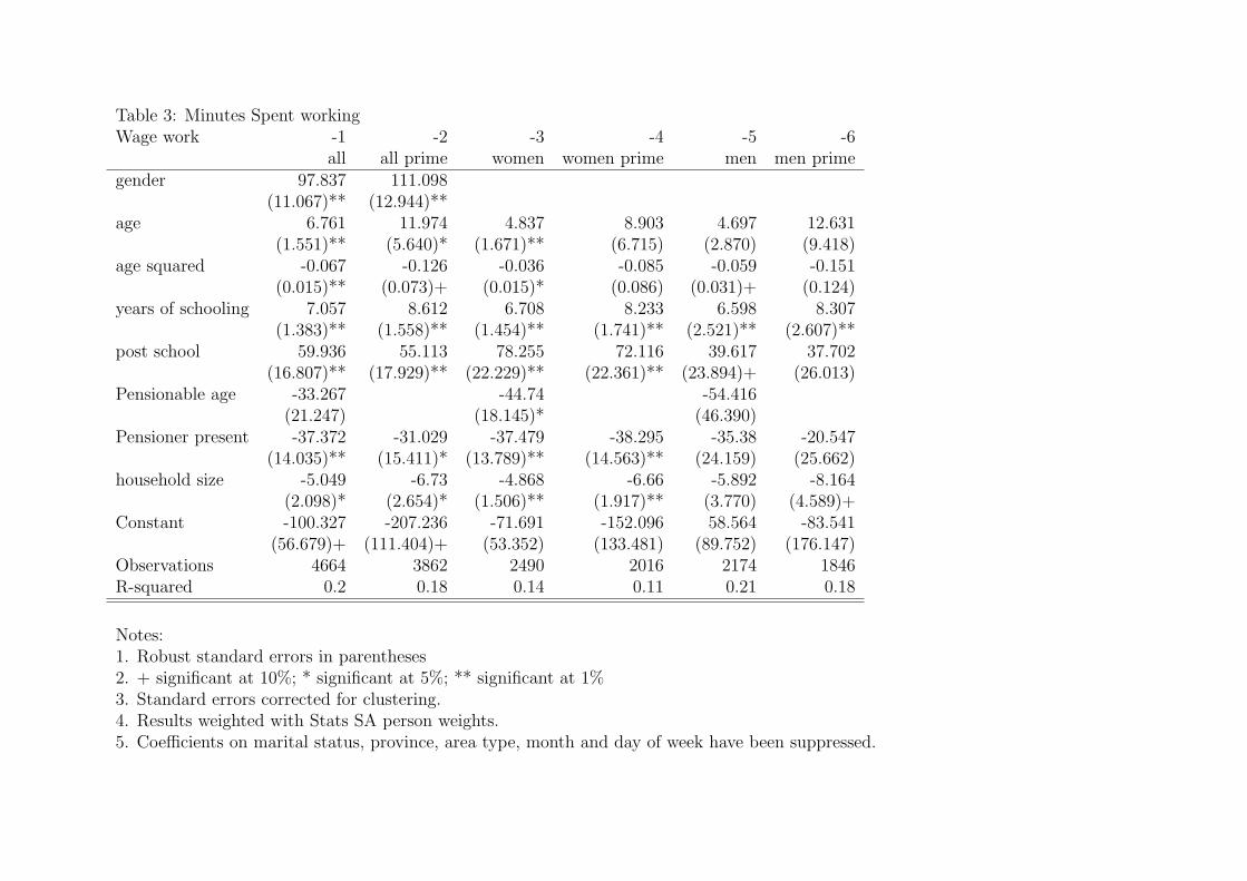
Table 3: Minutes Spent workingWage work -1 -2 -3 -4 -5 -6

all all prime women women prime men men primegender 97.837 111.098

(11.067)** (12.944)**age 6.761 11.974 4.837 8.903 4.697 12.631

(1.551)** (5.640)* (1.671)** (6.715) (2.870) (9.418)age squared -0.067 -0.126 -0.036 -0.085 -0.059 -0.151

(0.015)** (0.073)+ (0.015)* (0.086) (0.031)+ (0.124)years of schooling 7.057 8.612 6.708 8.233 6.598 8.307

(1.383)** (1.558)** (1.454)** (1.741)** (2.521)** (2.607)**post school 59.936 55.113 78.255 72.116 39.617 37.702

(16.807)** (17.929)** (22.229)** (22.361)** (23.894)+ (26.013)Pensionable age -33.267 -44.74 -54.416

(21.247) (18.145)* (46.390)Pensioner present -37.372 -31.029 -37.479 -38.295 -35.38 -20.547

(14.035)** (15.411)* (13.789)** (14.563)** (24.159) (25.662)household size -5.049 -6.73 -4.868 -6.66 -5.892 -8.164

(2.098)* (2.654)* (1.506)** (1.917)** (3.770) (4.589)+Constant -100.327 -207.236 -71.691 -152.096 58.564 -83.541

(56.679)+ (111.404)+ (53.352) (133.481) (89.752) (176.147)Observations 4664 3862 2490 2016 2174 1846R-squared 0.2 0.18 0.14 0.11 0.21 0.18

Notes:1. Robust standard errors in parentheses2. + significant at 10%; * significant at 5%; ** significant at 1%3. Standard errors corrected for clustering.4. Results weighted with Stats SA person weights.5. Coefficients on marital status, province, area type, month and day of week have been suppressed.

33

Table 4: Time spent on caregiving to other household membersCare for old Child care

-1 -2 -3 -4 -5 -6 -7 -8all all prime women prime men prime all all prime women prime men prime

gender -0.418 -0.343 -37.078 -40.394(0.307) (0.133)** (2.407)** (2.669)**

age 0.011 -0.008 -0.036 -0.022 -2.09 -3.168 -5.791 -1.315(0.059) (0.093) (0.166) (0.023) (0.592)** (1.944) (3.254)+ (1.493)

age squared 0.001 0 0.001 0 0.015 0.029 0.054 0.017(0.001) (0.001) (0.002) - (0.006)** (0.025) (0.041) (0.019)

years of schooling -0.068 -0.017 -0.034 0.005 0.229 0.236 0.329 0.255(0.060) (0.030) (0.054) (0.005) (0.373) (0.423) (0.754) (0.154)+

post school 0.419 0.336 0.704 -0.035 -4.095 -2.761 -3.899 1.852(0.421) (0.390) (0.817) (0.036) (4.369) (4.551) (8.870) (2.145)

Pensionable age -2.809 3.466(1.630)+ (5.857)

Pensioner present 0.341 0.042 0.055 -0.008 -8.979 -9.043 -21.464 6.098(0.606) (0.188) (0.353) (0.010) (3.483)* (3.852)* (5.981)** (3.619)+

household size -0.022 -0.023 -0.042 -0.003 2.406 2.45 4.553 0.454(0.021) (0.016) (0.030) (0.003) (0.574)** (0.664)** (1.118)** (0.318)

Constant 0.002 0.842 1.668 0.375 79.3 96.252 141.769 18.473(1.073) (1.718) (3.206) (0.380) (15.070)** (37.156)** (65.365)* (26.188)

Observations 4664 3862 2016 1846 4664 3862 2016 1846R-squared 0.01 0.01 0.01 0.01 0.13 0.14 0.08 0.04


34

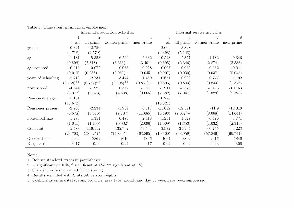
Table 5: Time spent in informal employmentInformal production activities Informal service activities


gender -0.321 -2.756 2.669 3.828(4.718) (4.579) (4.398) (5.148)

age 1.181 -5.358 -6.229 -2.332 0.548 2.357 4.182 0.346(0.896) (2.818)+ (3.663)+ (3.401) (0.695) (2.346) (2.874) (3.588)

age squared -0.013 0.072 0.088 0.028 -0.007 -0.032 -0.052 -0.011(0.010) (0.038)+ (0.050)+ (0.045) (0.007) (0.030) (0.037) (0.045)

years of schooling -2.713 -2.731 -3.474 -1.469 0.651 0.909 0.747 1.192(0.758)** (0.757)** (0.998)** (0.861)+ (0.696) (0.803) (0.843) (1.376)

post school -4.644 -1.923 0.367 -3.661 -1.911 -8.376 -8.496 -10.163(5.377) (5.328) (4.888) (9.065) (7.582) (7.047) (7.829) (9.326)

Pensionable age 5.151 10.278(13.672) (10.821)

Pensioner present -2.268 -2.234 -1.939 0.517 -11.082 -12.591 -11.9 -12.313(6.578) (6.585) (7.787) (11.685) (6.893) (7.637)+ (8.068) (14.641)

household size 1.276 1.351 0.475 2.418 1.231 1.527 -0.476 3.771(1.041) (1.195) (0.902) (2.096) (1.009) (1.353) (1.032) (2.313)

Constant 5.488 116.112 132.762 53.504 3.972 -35.934 -60.755 -4.223(23.700) (58.625)* (74.839)+ (63.895) (19.600) (43.959) (57.846) (69.741)



35

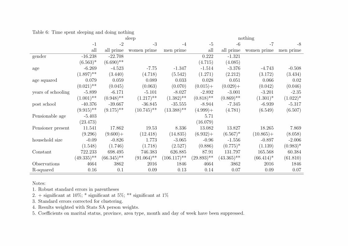
Table 6: Time spent sleeping and doing nothingsleep nothing


gender -16.238 -22.708 0.222 -1.321(6.563)* (6.690)** (4.715) (4.085)

age -6.269 -4.523 -7.75 -1.347 -1.514 -3.376 -4.743 -0.508(1.897)** (3.440) (4.718) (5.542) (1.271) (2.212) (3.172) (3.434)

age squared 0.079 0.059 0.089 0.033 0.028 0.051 0.066 0.02(0.021)** (0.045) (0.063) (0.070) (0.015)+ (0.029)+ (0.042) (0.046)

years of schooling -5.899 -6.171 -5.101 -8.027 -2.892 -3.001 -3.201 -2.35(1.001)** (0.948)** (1.217)** (1.382)** (0.818)** (0.869)** (1.301)* (1.022)*

post school -40.376 -39.667 -36.845 -35.555 -8.944 -7.345 -6.939 -5.317(9.915)** (9.175)** (10.745)** (13.388)** (4.999)+ (4.781) (6.549) (6.507)

Pensionable age -5.403 5.71(23.473) (16.079)

Pensioner present 11.541 17.862 19.53 8.336 13.082 13.827 18.265 7.869(9.296) (9.600)+ (12.418) (14.835) (6.932)+ (6.567)* (10.865)+ (8.058)

household size -0.09 -0.826 1.773 -3.065 -0.96 -1.556 -0.897 -2.006(1.548) (1.746) (1.718) (2.527) (0.886) (0.775)* (1.139) (0.983)*

Constant 722.233 698.495 746.383 626.885 87.91 131.797 165.568 60.384(49.335)** (66.345)** (91.064)** (106.117)** (29.893)** (43.365)** (66.414)* (61.810)



36

Table 7: Time spent socializingSocializing with family members Socializing with non-family members

-1 -2 -3 -4 -5 -6 -7 -8all all prime women prime men prime socnonfam all all prime women prime men prime

gender -13.456 -13.142 42.678 46.503(4.051)** (4.170)** (6.605)** (6.491)**

age -2.474 -6.006 -6.757 -4.835 0.576 -0.449 -2.111 2.103(1.243)* (2.651)* (3.832)+ (3.556) (0.800) (2.885) (2.445) (5.457)

age squared 0.027 0.069 0.076 0.056 -0.015 -0.003 0.021 -0.039(0.014)+ (0.034)* (0.048) (0.047) (0.008)+ (0.038) (0.031) (0.071)

years of schooling -3.526 -3.735 -3.792 -3.503 -1.081 -0.955 -0.408 -1.759(0.675)** (0.783)** (1.042)** (1.056)** (0.566)+ (0.589) (0.581) (1.038)+

post school 5.586 7.266 -6.585 19.13 -6.038 -5.712 -9.321 -5.99(6.200) (6.522) (8.122) (9.310)* (5.949) (6.596) (4.672)* (10.923)

Pensionable age -2.736 38.481(13.185) (13.312)**

Pensioner present 11.303 13.162 11.472 13.425 -8.17 -5.961 -2.938 -12.11(6.192)+ (6.544)* (8.920) (9.331) (6.141) (6.321) (5.509) (12.463)

household size 3.991 4.375 3.917 4.488 0.902 0.848 0.056 2.175(0.843)** (0.955)** (1.173)** (1.243)** (1.074) (1.108) (0.852) (1.885)

Constant 82.06 153.69 170.391 116.748 38.572 58.585 88.848 66.451(31.557)** (53.295)** (79.053)* (64.815)+ (22.250)+ (54.212) (47.829)+ (98.594)



37

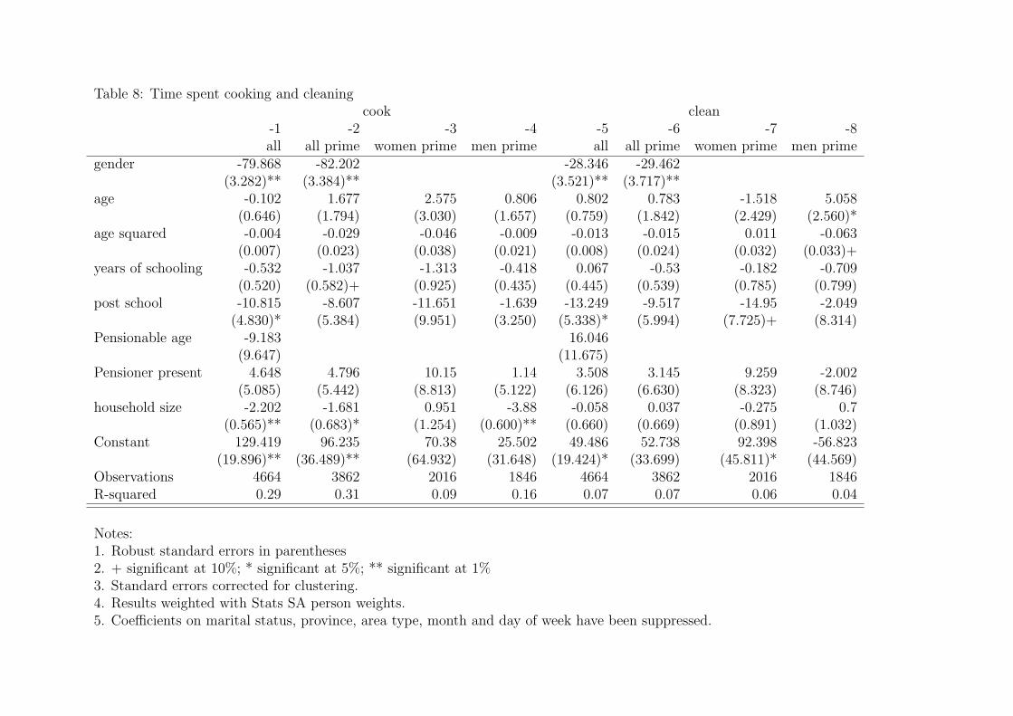
Table 8: Time spent cooking and cleaningcook clean


gender -79.868 -82.202 -28.346 -29.462(3.282)** (3.384)** (3.521)** (3.717)**

age -0.102 1.677 2.575 0.806 0.802 0.783 -1.518 5.058(0.646) (1.794) (3.030) (1.657) (0.759) (1.842) (2.429) (2.560)*

age squared -0.004 -0.029 -0.046 -0.009 -0.013 -0.015 0.011 -0.063(0.007) (0.023) (0.038) (0.021) (0.008) (0.024) (0.032) (0.033)+

years of schooling -0.532 -1.037 -1.313 -0.418 0.067 -0.53 -0.182 -0.709(0.520) (0.582)+ (0.925) (0.435) (0.445) (0.539) (0.785) (0.799)

post school -10.815 -8.607 -11.651 -1.639 -13.249 -9.517 -14.95 -2.049(4.830)* (5.384) (9.951) (3.250) (5.338)* (5.994) (7.725)+ (8.314)

Pensionable age -9.183 16.046(9.647) (11.675)

Pensioner present 4.648 4.796 10.15 1.14 3.508 3.145 9.259 -2.002(5.085) (5.442) (8.813) (5.122) (6.126) (6.630) (8.323) (8.746)

household size -2.202 -1.681 0.951 -3.88 -0.058 0.037 -0.275 0.7(0.565)** (0.683)* (1.254) (0.600)** (0.660) (0.669) (0.891) (1.032)

Constant 129.419 96.235 70.38 25.502 49.486 52.738 92.398 -56.823(19.896)** (36.489)** (64.932) (31.648) (19.424)* (33.699) (45.811)* (44.569)



38

Table 9: Time spent Watching TV and EatingTV Eat


gender -1.821 -3.922 7.596 6.722(4.527) (4.938) (2.033)** (2.211)**

age 0.391 -0.128 3.546 -4.481 0.23 1.149 1.036 1.272(0.834) (2.787) (4.056) (3.645) (0.470) (0.991) (1.145) (1.937)

age squared -0.004 0.005 -0.038 0.055 0.002 -0.008 -0.01 -0.005(0.008) (0.037) (0.055) (0.046) (0.005) (0.013) (0.015) (0.025)

years of schooling 4.43 4.523 4.48 4.856 -0.495 -0.466 -0.304 -0.635(0.738)** (0.801)** (1.135)** (1.126)** (0.256)+ (0.282)+ (0.328) (0.442)

post school 2.546 1.284 7.769 -3.201 2.621 3.006 4.541 2.779(8.400) (8.804) (10.768) (11.976) (2.663) (2.429) (2.817) (3.946)

Pensionable age -2.047 -7.998(12.050) (4.482)+

Pensioner present 4.041 3.826 2.368 7.166 8.56 7.643 4.957 10.916(8.363) (8.726) (9.810) (15.046) (2.898)** (3.036)* (3.291) (5.076)*

household size 2.687 3.299 4.188 2.509 -0.535 -0.52 -0.323 -0.639(1.141)* (1.252)** (1.393)** (1.897) (0.350) (0.418) (0.391) (0.715)

Constant 45.508 49.897 -27.734 131.237 46.584 29.793 40.649 24.473(23.837)+ (51.864) (74.447) (68.796)+ (13.109)** (20.081) (23.561)+ (34.987)



39

Income Eﬀects of Time Allocation in Poor South African ... · PDF fileIncome Eﬀects of...

Documents

Transcript of Income Eﬀects of Time Allocation in Poor South African ... · PDF fileIncome Eﬀects of...