IN RFID- E

The Pennsylvania State University

The Graduate School

The Harold and Inge Marcus

Department of Industrial and Manufacturing Engineering

MARKET-BASED DYNAMIC CONTROL OF

VEHICLE DEPLOYMENT AND SHIPMENT LOAD MAKEUP

IN RFID-ENALBED ENVIRONMENTS

A Thesis in

Industrial Engineering

by

Jindae Kim

© 2008 Jindae Kim

Submitted in Partial Fulfillment

of the Requirements

for the Degree of

Doctor of Philosophy

May, 2008

ii

The thesis of Jindae Kim was reviewed and approved* by the following:

Soundar R.T. Kumara

Allen E. and Allen M. Pearce Professor of Industrial Engineering

Thesis Advisor

Chair of Committee

A. Ravi Ravindran

Professor of Industrial Engineering

M. Jeya Chandra


Susan H. Xu

Professor of Management Science and Supply chain management

Shang-tae Yee

Program Manager, General Motors R&D Center

Special Member

Richard J. Koubek


Head of the Department of Industrial and Manufacturing Engineering

*Signatures are on file in the Graduate School

iii

ABSTRACT

For the past several decades, advances in manufacturing and supply chain

management have improved the business environment. Nonetheless, dynamics, such as

various unexpected disruptions and uncertainties, in business operations have significant

impact on decision-making efficiency. Adoption of wireless communication and sensor

technologies has facilitated real-time visibility of the operational dynamics in

manufacturing and supply chains. The availability of real-time information requires that

new decision-making strategy design should consider: (1) constantly changing

operational environment and (2) large amount of distributed information.

This thesis is motivated by a real world example relating to outbound logistics of

an automobile manufacturers’ supply chain. In specific, this thesis addresses the shipment

yard operations, such as vehicle deployment and shipment load makeup, where an RFID-

based wireless tracking system provides real-time information of vehicles. In order to

investigate the impact of RFID-based wireless tracking on the shipment yard operations,

new operational processes and corresponding decision-making models, which can

effectively utilize real-time vehicle information, are designed.

To support and solve new decision-making models for vehicle deployment and

shipment load makeup, this research introduces a market-based control mechanism,

which is supported by a multiagent-based information system architecture. As a market-

based control mechanism for vehicle deployment, an ascending price iterative auction

mechanism is designed. For shipment load makeup, two different market structures,

called a two-tier auctioning process and a single-tier auctioning process, are designed. In

order to control each local market in these auctioning processes, an iterative bundle

auction mechanism and an iterative high-bid auction mechanism are developed. The

performance of the market-based mechanisms is verified through intensive empirical

analysis supported by optimal solutions obtained by solving the mathematical

programming models. The results support point to high levels of solution quality and

iv

computational efficiency of the proposed market-based mechanism. Finally, the proposed

decision-making models and market-based control mechanisms improve the operational

performance of vehicle deployment and shipment load makeup by effectively responding

to the operational dynamics and incorporating the real-time information from the RFID-

based wireless tracking system.

v

TABLE OF CONTENTS

LIST OF TABLES ........................................................................................................... xi

LIST OF FIGURES ....................................................................................................... xiii

ACKNOWLEDGEMENTS ......................................................................................... xvii

CHAPTER 1. INTRODUCTION .....................................................................................1

1.1 Problem Domain Discussion....................................................................................2

1.1.1 Automobile Shipment Yard ............................................................................2

1.1.2 Radio Frequency Identification .......................................................................5

1.2 Market and Multiagent-based Approach to Decision-making for Shipment Yard

Operations ...............................................................................................................6

1.3 Research Objectives ................................................................................................7

1.4 Organization of the Thesis ......................................................................................7

CHAPTER 2. PROBLEM I: VEHICLE DEPLOYMENT - PRELIMINARIES ......10

2.1 Description of Vehicle Deployment Operations ....................................................10

2.2 Performance Measure for Vehicle Deployment ....................................................12

2.3 Dynamic Characteristics of Vehicle Deployment Planning ..................................13

2.4 Current Best Vehicle Deployment Practice ...........................................................15

CHAPTER 3. PROBLEM II: SHIPMENT LOAD MAKEUP – PRELIMINARIES

...............................................................................................................................18

3.1 Shipment Load Makeup at Automobile Manufacturer ..........................................18

3.2 Specifications of Shipment Load Makeup Environment .......................................20

3.2.1 Shipment Yard ..............................................................................................20

3.2.2 Local Dealer ..................................................................................................21

vi

3.2.3 Transportation Resource Division ................................................................22

3.2.4 Operational Facts in Shipment Load Makeup ..............................................23

3.3 Shipment Load Makeup Planning ..........................................................................23

3.3.1 Unique Operational Characteristics of Shipment Load Makeup Planning ...24

3.4 Mathematical Model of Shipment Load Makeup Planning ...................................25

3.4.1 Shipment Load Makeup Planning Environment ...........................................25

3.4.1.1 Planning Time Period ..........................................................................25

3.4.1.2 Set of Vehicles .....................................................................................27

3.4.1.3 Set of Trucks ........................................................................................28

3.4.1.4 Various Costs in Shipment Load Makeup ...........................................28

3.4.2 Integer Programming Models for Different Scenarios .................................31

3.4.2.1 Scenario 1: Vehicles are Indivisible ....................................................31

3.4.2.1.1 Decision Variables ......................................................................31

3.4.2.1.2 Objective Function of Shipment Load Makeup Planning...........32

3.4.2.1.3 Integer Programming Formulation for Scenario 1 ......................34

3.4.2.2 Scenario 2: Vehicles are Divisible .......................................................36

3.4.2.2.1 Decision Variables ......................................................................36

3.4.2.2.2 Objective Function of Shipment Load Makeup Planning...........36

3.4.2.2.3 Integer Programming Formulation for Scenario 2 ......................37

3.5 Computational Complexity and Limitations in Real Environment .......................39

3.5.1 Computational Complexity of Shipment Load Makeup Planning ................39

3.5.2 Limitations in a Real Shipment Yard Environment ......................................42

CHAPTER 4. BACKGROUND LITERATURE SURVEY .........................................44

4.1 RFID-enabled Applications ...................................................................................44

4.1.1 RFID in Various Business Areas ..................................................................45

4.1.2 RFID in Supply Chains .................................................................................46

4.2 Management of Automobile Shipment Yard .........................................................48

4.3 Market-based Control Mechanism for Resource Allocation ................................52

vii

CHAPTER 5. OVERALL SOLUTION APPROACH .................................................54

5.1 Design of New Operational Process with Real-time Information from RFID ......54

5.2 Design of Multiagent-based Decision-making Framework ...................................54

5.3 Design of Market-based Control Mechanism ........................................................55

CHAPTER 6. VEHICLE DEPLOYMENT – SOLUTION METHODOLOGY ........58

6.1 Vehicle Deployment in RFID-enabled Shipment Yard .........................................58

6.1.1 Initial Decision for Vehicle Deployment ......................................................59

6.1.2 Updating Vehicle Deployment Decisions .....................................................61

6.2 Multiagent-based Decision-making Framework ....................................................63

6.2.1 Design of Agents...........................................................................................63

6.3 Market-based Control Mechanism .........................................................................64

6.3.1 Auction Heuristic Mechanism ......................................................................64

6.3.2 Ascending Price Iterative Auction Mechanism ............................................67

6.4 Design of Utility Function for Vehicle Agent .......................................................70

CHAPTER 7. EMPIRICAL ANALYSIS OF VEHICLE DEPLOYMENT ...............74

7.1 Experimental Setup ................................................................................................74

7.1.1 Experimental Conditions ..............................................................................75

7.2 Consolidated Operational Time .............................................................................76

7.3 Shipment Yard Utilization .....................................................................................77

7.3.1 Utilization Rate of Parking Slot ....................................................................78

7.3.2 Frequency of Parking Slot Utilization ..........................................................81

7.4 Labor Consumption ...............................................................................................85

7.5 Summary of Empirical Analysis ............................................................................87

CHAPTER 8. SHIPMENT LOAD MAKEUP – SOLUTION METHODOLOGY I

...............................................................................................................................88

8.1 Shipment Load Makeup in RFID-enabled Shipment Yard....................................88

8.2 Shipment Load Makeup Decision in RFID-enabled Shipment Yard ....................90

viii

8.2.1 Shipment Load Makeup Decision in Scenario 1...........................................90

8.2.2 Shipment Load Makeup Decision in Scenario 2...........................................92

8.3 Shortcomings of Shipment Load Makeup Decision Model in a Distributed Large

Scale Environment ................................................................................................95

8.4 Multiagent Architecture for Shipment Load Makeup in RFID-enabled Shipment

Yard .......................................................................................................................95

CHAPTER 9. SHIPMENT LOAD MAKEUP – SOLUTION METHODOLOGY II

...............................................................................................................................99

9.1 The First Round Local Auction .............................................................................99

9.1.1 Construction of the First Round Local Auction Market ...............................99

9.1.2 Descriptions of Bundle Expression for Identical Items ..............................101

9.1.3 Overall Procedure of Iterative Bundle Auction Mechanism.......................105

9.1.4 Dealer Agent Bidding Strategy ...................................................................106

9.1.4.1 Exclusive-Or (XOR) Bid ....................................................................106

9.1.4.2 Myopic Best-Response Bidding Strategy ..........................................107

9.1.4.3 Second-Chance Bidding Strategy ......................................................108

9.1.5 Temporary Allocation of Bundles ..............................................................110

9.1.5.1 Winner Determination Problem .........................................................110

9.1.5.2 Refinement of Winner Determination Problem .................................111

9.1.5.3 Effective Winner Determination Algorithm ......................................113

9.1.6 Strategy of BA for Updating Asking Price .................................................116

9.1.7 Example of Iterative Bundle Auction .........................................................118

9.2 Design of Utility Function for Dealer Agent .......................................................121

9.3 The Second Round Central Auction ....................................................................122

9.3.1 Structure of the Second Round Central Auction Market ............................122

9.3.2 Utility Value for Block Agent.....................................................................124

9.3.3 Block Agent Bidding Strategy ....................................................................125

9.3.4 Updating Temporary Allocation .................................................................125

9.3.5 Updating Asking Price for Truck ................................................................126

ix

9.3.6 Market Termination ....................................................................................126

CHAPTER 10. SHIPMENT LOAD MAKEUP –SOLUTION METHODOLOGY III

.............................................................................................................................128

10.1 Dealer Agent in Single-Tier Auctioning Process ...............................................128

10.2 Construction of the Direct Local Auction Market .............................................128

10.3 Iterative High-Bid Auction Mechanism.............................................................131

10.3.1 Dealer Agent Bidding Strategy .................................................................132

10.3.2 Utility Value for Dealer Agent .................................................................133

10.3.3 Winner Determination at Each Iteration ...................................................134

10.3.4 Revenue of Proxy Agent from Auction Market ........................................135

10.3.5 Example of Iterative High-Bid Auction ....................................................135

10.4 Determination of Final Allocations of Items .....................................................138

CHAPTER 11. EMPIRICAL ANALYSIS OF SHIPMENT LOAD MAKEUP .....140

11.1 Experimental Setup ............................................................................................140

11.1.1 Simulator for Shipment Load Makeup .....................................................140

11.1.2 Generation of Shipment Load Makeup Instances .....................................143

11.2 Performance of Market-based Approach for Shipment Load Makeup ..............146

11.2.1 Performance of Two-tier Auctioning Process for Scenario 1 ...................147

11.2.2 Performance of Single-tier Auctioning Process for Scenario 2 ................151

11.3 Scalability of Market-based Decentralized Approach .......................................155

11.3.1 Effect of Number of Blocks ......................................................................157

11.3.2 Effect of Number of Dealers .....................................................................161

11.3.3 Effect of Number of Vehicles ...................................................................165

11.3.4 Effect of Number of Vacancies on a Truck ..............................................169

11.4 Summary of Empirical Analysis ........................................................................173

CHAPTER 12. CONCLUSIONS AND FUTURE RESEARCH ...............................175

12.1 Contributions......................................................................................................175

x

12.2 Managerial Implications ....................................................................................178

12.3 Future Research ................................................................................................179

BIBLIOGRAPHY ..........................................................................................................183

xi

LIST OF TABLES

Table 6.1: Auction heuristic mechanism for updating vehicle deployment

decision.....................................................................................................66

Table 6.2: Ascending price iterative auction mechanism for updating vehicle

deployment decisions ...............................................................................70

Table 6.3: Instance of a shipment loading schedule that follows a high-priority-first-

loaded (HPFL) rule...................................................................................72

Table 7.1: Classification of vehicle deployment models...........................................75

Table 7.2: Average operational time (unit time) for deployment of a single vehicle

..................................................................................................................77

Table 9.1: DA valuations for vacancies on a truck .................................................102

Table 9.2: New representations of DA valuations for identical vacancies (items) .103

Table 9.3: DAs with their bidding information: bidding price and bundle size ......115

Table 9.4: The sorted list of the DAs by STEP-1 ....................................................116

Table 9.5: The number of vehicles and a value of each bundle ..............................118

Table 9.6: Example of the iterative bundle auction mechanism: For the first round

local auction market, where minimum bidding price increment

is 10 ....................................................................................................120

Table 10.1: The fixed cost for visiting and unloading and the values of vehicles ....136

Table 10.2: Small size example of the iterative high-bid auction mechanism ..........137

Table 11.1: Controllable shipment load makeup configuration parameter ...............144

Table 11.2: Controllable shipment load makeup cost parameter ..............................145

Table 11.3: Random generation of vehicles in a shipment yard ...............................146

Table 11.4: Input parameters values used for generating shipment load makeup

instances .................................................................................................147

Table 11.5: Description of each column in the experiment result table ....................148

Table 11.6: Experimental results of the two-tier auctioning process for the shipment

load makeup scenario 1 ..........................................................................149

xii

Table 11.7: Experimental results of the single-tier auctioning process for the

shipment load makeup scenario 2 ..........................................................153

Table 11.8: Experiment results of testing the effect of varying number of blocks on

the performance of the local auction mechanism in two-tier auctioning

process (scenario 1) ...............................................................................158

Table 11.9: Experiment results of testing the effect of varying number of blocks on

the performance of the local auction mechanism in single-tier auctioning


Table 11.10: Experiment results of testing the effect of varying number of dealers on



Table 11.11: Experiment results of testing the effect of varying number of dealers on



Table 11.12: Experiment results of testing the effect of varying number of vehicles on



Table 11.13: Experiment results of testing the effect of varying number of vehicles on



Table 11.14: Experiment results of testing the effect of varying number of vacancies

on a truck on the performance of the local auction mechanism in two-tier

auctioning process (scenario 1) .............................................................170

Table 11.15: Experiment results of testing the effect of varying number of vacancies

on a truck on the performance of the local auction mechanism in single-

tier auctioning process (scenario 2) .......................................................172

xiii

LIST OF FIGURES

Figure 1.1: Shipment yard of an automobile manufacturer ..........................................3

Figure 1.2: Research road map and thesis organization ...............................................9

Figure 2.1: Illustration of elementary operations for deployment of vehicle i ...........11

Figure 2.2: Current best vehicle deployment practice ................................................16

Figure 3.1: Supply chains of an automobile manufacturer .........................................19

Figure 3.2: Key participants and their managerial objectives in shipment load

makeup .....................................................................................................20

Figure 3.3: Local dealers clustered into a number of blocks ......................................21

Figure 3.4: Shipment load makeup planning time period ...........................................26

Figure 3.5: Dwell time of a vehicle ............................................................................28

Figure 3.6: Costs in shipment yard .............................................................................29

Figure 3.7: Costs for vehicle v in local dealer vd .......................................................30

Figure 3.8: The growth of solution space as the average number of vehicles rt

V

increases ( , ,1 2 3R and ,r 4 r R ) ........................................40

Figure 3.9: The growth of solution space as the number trucks R increases (rt

8V

and ,r 4 r R ) ...............................................................................41

Figure 5.1: Overall solution approach ........................................................................57

Figure 6.1: Information architecture for RFID-enabled shipment yard......................59

Figure 6.2: The set of available parking slots for a vehicle deployment decision in (a)

the current best vehicle deployment model, and (b) the initial vehicle

deployment decision model ......................................................................61

Figure 6.3: Illustration of design for ascending price iterative auction mechanism

which includes a dummy vehicle agent....................................................68

Figure 7.1: Structure and size of the shipment yard use for the experiments .............76

Figure 7.2: Utilization rate of parking slot in CVD ....................................................79

Figure 7.3: Utilization rate of parking slot in RVDID

.................................................79

xiv

Figure 7.4: Utilization rate of parking slot in RVDID+AH

............................................80

Figure 7.5: Utilization rate of parking slot in RVDID+IA

...........................................80

Figure 7.6: Average utilization rate of the parking slots (50 parking slots) in each

parking slot column .................................................................................81

Figure 7.7: Frequency of parking slot utilization in CVD .........................................82

Figure 7.8: Frequency of parking slot utilization in RVDID

......................................83

Figure 7.9: Frequency of parking slot utilization in RVDID+AH

................................83

Figure 7.10: Frequency of parking slot utilization in RVDID+IA

.................................84

Figure 7.11: Average number of vehicles moved into the parking slots (50 parking

slots) in each parking slot column ..........................................................85

Figure 7.12: Average labor consumption of a yard operator with different vehicle

deployment models .................................................................................86

Figure 7.13: Average labor consumption of a trucker with different vehicle

deployment models .................................................................................87

Figure 8.1: Illustrative comparison between shipment load makeup planning model

and real-time shipment load makeup decision model .............................89

Figure 8.2: Interaction among the YA, the RFID data server, and DAs ...................97

Figure 9.1: Construction of the first round local auction markets ...........................100

Figure 9.2: Growth of the maximum number of possible bundles ..........................105

Figure 9.3: Overall procedure of the iterative bundle auction mechanism for the first

round local auction market ....................................................................106

Figure 9.4: Fundamental procedure of the second-chance bidding strategy in the

first round local auction market ............................................................110

Figure 9.5: Structure of the second round central auction market ..........................124

Figure 9.6: The overall procedure of the auction mechanism in the second round

central auction market ...........................................................................127

Figure 10.1: Construction of a temporary economy and multiple direct local auction

markets ................................................................................................130

Figure 10.2: Overall procedure of the iterative high-bid auction mechanism ...........132

xv

Figure 10.3: RA’s final allocations determined by results of all the local auction

markets ..................................................................................................139

Figure 11.1: Structure of shipment load makeup simulator .....................................141

Figure 11.2: Example of LINDO input for Scenario 1, which is automatically

generated by problem instance generator (5 blocks, 5 dealers per block,

and 50 vehicles) ...................................................................................142

Figure 11.3: Example of LINDO input Scenario 2, which is automatically generated

by problem instance generator (5 blocks, 5 dealers per block, and 50

vehicles) ...............................................................................................143

Figure 11.4: Optimality of the two-tier auctioning process solution varying the

average number of dealers per block and the average number of

vehicles per dealer: (a) the average optimality, (b) ANo_D = 10, (c)

ANo_D = 20, (d) ANo_D = 30, (e) ANo_D = 40, and (e) ANo_D = 50 ..

.............................................................................................................150

Figure 11.5: Computational efficiency of the two-tier auctioning process varying the

average number of dealers per block ...................................................151

Figure 11.6: Optimality of the single-tier auctioning process solution varying the

average number of dealers per block and the average number of


ANo_D = 20, (d) ANo_D = 30, (e) ANo_D = 40, and

(e) ANo_D = 50 ...................................................................................154

Figure 11.7: Computational efficiency of the single-tier auctioning process varying

the average number of dealers per block and the average number of


ANo_D = 20, (d) ANo_D = 30, (e) ANo_D = 40, and

(e) ANo_D = 50 ...................................................................................155

Figure 11.8: Effect of the number of blocks on the performance of the local auction

mechanism for scenario 1: (a) average number of iterations, (b) average

computation time, and (c) average computation time per iteration .....159

xvi

Figure 11.9: Effect of the number of blocks on the performance of the local auction

mechanism for scenario 2: (a) average number of iterations, (b) average

computation time, and (c) average computation time per iteration .....161

Figure 11.10: Effect of the number of dealers on the performance of the local auction

mechanism for scenario 1 ....................................................................163

Figure 11.11: Effect of the number of dealers on the performance of the local auction

mechanism for scenario 2 ...................................................................165

Figure 11.12: Effect of the number of vehicles on the performance of the local

auction mechanism for scenario 1 ......................................................167

Figure 11.13: Effect of the number of vehicles on the performance of the local

auction mechanism for scenario 2 ......................................................169

Figure 11.14: Effect of the number of vacancies on a truck on the performance of the

local auction mechanism for scenario 1 .............................................171

Figure 11.15: Effect of the number of vacancies on a truck on the performance of the

local auction mechanism for scenario 2 .............................................173

xvii

ACKNOWLEDGEMENTS

I would like to express my gratitude to my advisor, Dr. Soundar Kumara, for his

direction, assistance, and encouragement throughout my Ph.D. study at the Pennsylvania

State University. He is an enthusiastic researcher, a patient teacher, and most of all a

warm-hearted person. I have tried to learn all of his virtues and insightful perspectives for

the last five years since I started working with him. I also wish to thank Dr. A. Ravi

Ravindran, Dr. M. Jeya Chandra, Dr. Susan H. Xu, and Dr. Shang-tae Yee, for their

intellectual guidance and suggestions during my research.

In finishing my Ph.D. study, I would like to give special thanks to Dr. Honghee

Lee (at the Inha University). The work experience with him in my M.S. study indeed

made a great contribution and motivation toward my finishing Ph.D. study. Thanks are

also due to my senior, Dr. Yonghan Lee, Dr. Seogcheon Lee, Dr. Younho Hong, and Mr.

Changsoo Ok, for their invaluable comments and encouragement. Special thanks should

be given to my student colleagues who have been with me all the way and helped me in

many ways.

I am especially indebted to my wife Junghwa and my sons Minwoo and Minsuh

for their patience. They had to sacrifice many aspects of their lives due to my Ph.D. study

in the U.S. Words alone cannot express how much I feel sorry and how much I love

them. I also would like to thank my parents, sister, and brother in law, from the bottom of

my heart, for their prayers and confidence in me. I am really proud of them all. Finally, I

want to praise God for His blessing me.

1

Chapter 1

Introduction

For the past several decades, advances in manufacturing and supply chain

management have improved to a great extent the business performance of companies.

Nonetheless, a gap, still exists between plan and execution because of dynamics, such as

various unexpected disruptions and uncertainties, in business operations. Two important

capabilities are essential to fill this gap: One is to quickly detect the operational dynamics

in business operations, and the other is to effectively share that information with business

partners.

Huang et al. (2003) contend that many problems in dynamic operational

environments have their resolutions in timely information sharing among operational

members. For the dimension of timeliness, lateness and inaccuracy in sharing information

are identified as one of the major causes of performance degradation in decision-making

for manufacturing companies (Lee et al., 1997; Hong-Minh et al., 2000), while the

information exchange in real-time has been proposed to improve operational performance

(Karaesmen, 2002). Thus, the requirements for decision-making systems in order to

achieve management goals are that they should be adaptable and flexible enough to

process real-time information and responsive to the dynamic environment.

Recently, as a result of adoption of wireless communication and sensor

technologies in various real-world environments of manufacturing and supply chains,

real-time visibility of the operational dynamics improves and the enhanced visibility

allows the design of new decision-making strategies. Due to real-time information

availability, new decision-making strategy design should consider: (1) constantly

changing operational environments, (2) large amounts of distributed information

processing, (3) flexibility, and (4) real-time visibility of information on inventories,

resources, etc.

2

1.1 Problem Domain Discussion

This thesis addresses the decision-making problems of vehicle deployment and

shipment load makeup in an automobile shipment yard where wireless tracking is

enabled. The formal problem specifications, including optimization models, for vehicle

deployment and shipment load makeup are discussed in Chapters 2 and 3, respectively.

This section introduces a shipment yard of an automobile manufacturer and a Radio

Frequency IDentification (RFID)-enabled real-time wireless tracking system.

1.1.1 Automobile Shipment Yard

In the supply chains of automobile manufacturers, management of shipment yard

operations is a very important activity. Everyday, thousands of vehicles are produced at

an assembly plant. Once a vehicle is completely assembled, it passes through required

inspection in an inspection area and moves into a corresponding buffer area in a shipment

yard as shown in Figure 1.1. The shipment yard stores a number of finished vehicles until

they are shipped for delivery. The vehicles in the shipment yard are delivered via various

transportation modes, such as truck with trailer1 or train, to numerous local dealers

throughout the nation and regional vehicle distribution centers.

1 For this research, “truck” is the term of convenience for “truck with a trailer.”

3

Fig. 1.1: Shipment yard of an automobile manufacturer.

The main operations in the shipment yard, vehicle deployment and shipment load

makeup, are basically subsidiary or supportive processes of the automobile

manufacturer’s outbound logistics. Based on an understanding of automobile

manufacturer’s shipment yard operations, vehicle deployment and shipment load makeup

are defined as:

Definition 1.1. (vehicle deployment) Vehicle deployment in an automobile shipment

yard consists of the operations of (1) moving vehicles released from an assembly plant to

available parking slots in a general truck or train buffer of the shipment yard and then, (2)

moving vehicles in the general buffer into designated loading locations based on a

shipment loading schedule. Decision-making in vehicle deployment is to assign a vehicle

released from the assembly plant to one of the available parking slots in the general

buffer in order to achieve a required managerial objective in the shipment yard.

4

Definition 1.2. (shipment load makeup) Shipment load makeup in an automobile

shipment yard is the operation of loading a set of vehicles from a general truck or train

buffer of the shipment yard onto a truck or a train for delivering vehicles to their

destinations. Decision-making in shipment load makeup involves assigning a set of

vehicles to a set of available vacancies on a truck or a train without violating any

operational constraint while obtaining multiple managerial objectives predefined from

related functional divisions, such as the shipment yard, local dealers, and transportation

resource division.

The unique characteristics of the operational and decision-making environments

for vehicle deployment and shipment load makeup are:

� Inevitable dynamics: Due to frequent changes and uncertainties in vehicle

production, transportation resources, and market situations, available vehicles and

parking slots in the shipment yard and a transportation resource’s schedule

frequently change. As a result, original plans, based on estimation, are seldom

accomplished as planned.

� Large amounts of distributed information: As functional entities in vehicle

deployment and shipment load makeup, such as vehicles, shipment yard, local

dealers, and transportation resource division, are distributed organizationally,

geographically, and/or computationally, these local entities maintain their own

local information. Consequently, as the scale of shipment yard operations grows,

more and more information must be managed and processed.

� Self-interestedness: A shipment yard management goal is achieved throughout a

series of functional entities, such as shipment yard, dealers, and transportation

resource division. Usually these entities have their own objectives in the shipment

yard operations. As a result, coordination is necessary to solve conflicts among

self-interested entities.

5

� Frequent and prompt decision-making: Decision-making in vehicle deployment

and shipment load makeup is required frequently and should provide adaptable

solutions promptly.

1.1.2 Radio Frequency Identification

Radio Frequency IDentification (RFID) is a sensor technology that enables

wireless data communication for automatic identification of objects. An RFID system

consists of two basic components: the RF tag and the RFID reader. The RF tag, also

known as a transponder, typically contains a silicon chip that can hold a certain amount

of data and an antenna that broadcasts the data to a remote reader device. The RFID

reader, sometimes referred to as an interrogator, communicates with multiple RF tags by

means of sending and receiving radio frequency waves. Finally, the RFID reader sends

the data collected from RF tags to an RFID data server that compiles the information

(Gaukler, 2005; Holler, 2007).

Recently, owing to the driving forces of the U.S. Department of Defense and Wal-

Mart Inc., Radio Frequency IDentification (RFID) and wireless communication

technologies have been widely introduced into real-world supply chains. Also, the

EPCglobal consortium (http://www.epcglobalinc.org/), transferred from the Auto-ID

Center, has been playing a key role in stimulating the use of RFID for supply chains

(Sbihli, 2002; Paqani, 2005).

RFID technology, leveraged with other wireless technologies like wireless local

area network (WLAN), provides a real-time visibility of dynamics by enabling to identify

and track all the entities, including resources and finished products from supply chains,

and by allowing instant identification and automatic information transfer of object-states

(Karkkajnen and Holmstrom, 2002; Karkkajnen and Holmstrom, 2004; Angeles, 2005).

Providing visibility of the dynamics of supply chain entities to decision-making systems

in an automated and timely manner results in several advantages: (1) provides new

opportunities to better control the supply chain, (2) allows performing routine and manual

tasks more efficiently at much lower cost, and (3) offers real-time information of

6

operational-level transactions to corporate-level information systems to better shape

supply chain planning and execution, in particular, production and scheduling (Datta and

Viguier, 2000; Hanebeck and Tracey 2003; Walker, 2005).

This thesis introduces an RFID technology for an automobile shipment yard and

investigates the impact of the RFID technology on traditional operations in that shipment

yard. By virtue of the RFID technology, the product information including its current

location is provided in real-time, and the lack of communication problems among the

supply chain members related to the shipment yard operations become resolved. For the

new shipment yard environment, where the RFID technology is in place and the

enhanced operations are allowed, new decision-making strategies should be

considerations for achieving better shipment yard management goals.

1.2 Market and Multiagent-based Approach to Decision-making for Shipment Yard

Operations

Due to the unique characteristics of the decision-making environment for the

shipment yard operations and the availability of large amounts of real-time information,

as discussed in the previous Sections 1.1.1 and 1.1.2, respectively, modeling the decision-

making processes for vehicle deployment and shipment load makeup as a market-based

negotiation process is very attractable. The market-based negotiation process is facilitated

by the introduction of a mulitagent-based computational framework. The important

aspects regarding the market and multiagent-based approach are:

� The market-based control mechanism and multiagent-based architecture are well

known as they inherently follow a decentralized framework in nature. Thus, the

decision-making processes for large scale vehicle deployment and shipment load

makeup can be naturally modeled by these approaches.

� Each functional entity in vehicle deployment and shipment load makeup can

easily be modeled as an autonomous agent that maintains its local information and

tries to achieve its own objective.

7

� The market and multiagent-based approach is suitable for modeling and

processing a large amount of information in a distributed manner, so the decision-

making processes that should incorporate a large amount of real-time information

provided by an RFID system can be efficiently implemented.

� The market and multiagent-based approach is adaptable and flexible, thereby

reducing the implementation effort in response to the frequently changing

shipment yard operational environment (Lee, 2002).

1.3 Research Objectives

This research studies automobile manufacturer’s shipment yard operations where

an RFID system provides enhanced visibility of operational dynamics and uncertainties

by providing real-time information of vehicles in the shipment yard. The main goal of the

research is to investigate the impact of RFID technology on shipment yard operations and

corresponding decision-making strategies. Achieve this goal requires addressing the

following main research objectives.

� Define decision-making models for optimizing an automobile manufacturer’s

shipment yard operations, vehicle deployment and shipment load makeup, by

designing mathematical programming models.

� Design new shipment yard operational processes and corresponding decision-

making models, which can effectively utilize real-time information obtained from

an RFID system.

� Design a multiagent-based information system architecture to support the new

decision-making models in the RFID-enabled shipment yard.

� Develop auction mechanisms as a market-based control approach to solve the new

decision-making models (i.e., optimization problems) for vehicle deployment and

shipment load makeup processes in the RFID-enabled shipment yard.

1.4 Organization of the Thesis

8

The operational specifications and related decision-making models for vehicle

deployment and shipment load makeup are discussed in Chapters 2 and 3, respectively.

Chapter 4 briefly reviews the related background literature, and Chapter 5 discusses the

design of an overall solution methodology. Chapter 6 presents a new vehicle deployment

process in the RFID-enabled shipment yard and a market-based mechanism for the new

process. The computational experiments with the results analysis appear in Chapter 7.

Chapter 8 presents a shipment load makeup process and a multiagent-based information

framework in the new shipment yard environment. Two different market-based control

mechanisms for the new shipment load makeup processes are presented in Chapters 9 and

10, and Chapter 11 discusses the computational experiments with the results. Finally,

conclusions and possible extensions of this research work are the subject of Chapter 12.

Figure 1.2 summarizes the road map of the research and this thesis’s organization.

9

Fig. 1.2: Research road map and thesis organization.

Introduction

� Automobile shipment yard � RFID technology

Vehicle deployment

� Operational specifications � Mathematical model � Limitations

Shipment load makeup

Conclusions � Contributions � Managerial implications � Future research

Chapter 12

Chapter 1

Chapter 2 Chapter 3

� Operational specifications � Mathematical model � Limitations

Vehicle deployment: Solution methodology

� New deployment process � Mathematical model � Multiagent framework � Market-based mechanism

(Iterative auction)

Chapter 6

Shipment load makeup: Solution methodology I � New operational process � Mathematical model � Multiagent framework

Chapter 8

Vehicle deployment: Empirical analysis

� Experimental setup � Empirical analysis

Chapter 7

Solution methodology II

� Two-tier auctioning process

Solution methodology III

� Single-tier auctioning process

Shipment load makeup: Empirical analysis

� Experimental setup � Empirical analysis

Chapter 11

Chapter 9 Chapter 10

Literature survey

� RFID applications � Multiagent and market

based approach

Chapter 4

Overall solution approach

� New operational process � Multiagent framework � Market-based

Chapter 5

10

Chapter 2

Problem I: Vehicle Deployment - Preliminaries

This chapter details the vehicle deployment process in a shipment yard of an

automobile manufacturer by describing the operations and defining an associated

performance measures. In order to discuss dynamic characteristics of the vehicle

deployment process, the mathematical model for vehicle deployment is presented along

with the limitations for applying the model to a real shipment yard environment. At the

end of this chapter, the best available vehicle deployment practice in a current shipment

yard environment is presented for the purpose of comparing vehicle deployment

performance.

2.1 Description of Vehicle Deployment Operations

Once a vehicle is released from an assembly plant, it stays at a temporary buffer

of a shipment yard as illustrated in Figure 1.1. Subsequently, the vehicle moves to a

general truck buffer or a general train buffer according to its pre-determined delivery

transportation mode. The general buffers store a number of vehicles until they move to

loading buffers where they are loaded onto trucks or trains for delivery. In fact, every

finished vehicle has its delivery destination, with a corresponding transportation mode,

assigned by a delivery schedule. Since train transportation limits delivery destinations,

and consequently, the nature of the vehicle deployment process is relatively less dynamic,

this study focuses on truck transportation only. Before actual loading onto trucks, the

vehicles first move from the general buffer to a truck loading buffer consisting of many

loading locations. The truck in each loading location has a particular delivery destination,

e.g., Philadelphia, PA.

Vehicle deployment consists of two main operations: (1) yard operators move

vehicles from the temporary buffer to available parking slots in the general buffer, and

11

(2) truckers move vehicles from the general buffer to designated loading locations in the

loading buffer. For a single vehicle deployment, these two main operations are further

divided into four elementary operations. Figure 2.1 illustrates these elementary operations

where operations, EO-I and EO-II, are performed by yard operators, and EO-III and EO-

IV, are performed by truckers.

Fig. 2.1: Illustration of elementary operations for deployment of vehicle i.

EO-I : Driving vehicle i from vehicle pick up point Q in the temporary buffer to

allocated parking slot bi in the general buffer.

EO-II : Riding back to the temporary buffer from parking slot bi. Since the distance

between the temporary buffer, located near the assembly plant, and the

general buffer located in the shipment yard is quite long, a yard operator

comes back to the temporary buffer via a transportation utility like a van.

EO-III : Walking from loading location Li for vehicle i in the loading buffer to

parking slot bi to pick up the vehicle i. Since the general buffer and the

loading buffer adjoin, a trucker moves from the loading buffer to the general

buffer by walking.

EO-IV : Driving vehicle i from parking slot bi to its loading location Li

12

2.2 Performance Measure for Vehicle Deployment

A vehicle deployment problem is a problem of allocating one of the available

parking slots in the general buffer to a newly produced vehicle by minimizing handling

time, i.e. a consolidated operational time, defined as the total time required for the four

elementary operations listed earlier.

The consolidated operational time mainly depends on driving, riding, and walking

distance matrices between every pair of locations in the shipment yard. However, the

matrices cannot be easily generated by hand due to the size of a typical shipment yard

which may have more than a thousand parking slots. Because of that, a model may

consist of an approximation of driving, riding, and walking distances (i.e., rectilinear

distance for driving and riding, and Euclidian distance for walking).

Driving and riding distances can be approximately calculated by rectilinear

distance because the general buffer is filled with vehicles, and both vehicles and the van

can move only along accessible roads in the shipment yard. For example, driving and

riding distances between two locations m and n, denoted by ,dD m n and ,rD m n ,

are calculated by:

where ix and iy denote an x-coordinate and a y-coordinate of location i, respectively.

Computation of walking distance between two locations m and n, as ,wD m n

uses Euclidian distance:

Using the approximated distance matrices, operational times for a yard operator

and a trucker for deployment of vehicle i are calculated as:

, , m n m nd rD m n D m n x x y y= = − + − (2.1)

( ) ( ),1 22 2m n m n

wD m n x x y y = − + − (2.2)

13

where ds , rs , and ws are unit speeds for driving, riding, and walking, respectively. In

Equation (2.3) waitt denotes the amount of time for a yard operator to wait for a van, and

loadt in Equation (2.4) denotes the time a trucker uses to load a vehicle onto a truck.

Finally, the consolidated operational time for deployment of vehicle i,

( ),i iCOT L b , is defined as the sum of operational times for both a yard operator and a

trucker.

2.3 Dynamic Characteristics of Vehicle Deployment Planning

Because release of finished vehicles from the assembly plant to the temporary

buffer is sequential, over time, the decisions for corresponding parking slot allocations

are also made by solving a series of vehicle deployment problems, and each vehicle

deployment decision should be made interactively with other vehicle deployment

decisions. In other words, a vehicle deployment decision made in the current decision

epoch affects later decisions, and in addition, the overall status of the yard could become

uncertain, over time, due to changes in vehicle production schedules, truck arrival

schedules, and the immediate yard status.

To present a sequence of interrelated vehicle deployment decisions, ( )* ttf B is

the minimum value of the total consolidated operational time for the vehicles released,

where tB represents the set of available parking slots in the general buffer at time t. The

( ) , ,d i r iY i wait

d r

D Q b D b QOT b t

s s

= + +

(2.3)

( ) , ,, w i i d i i

T i i loadw d

D L b D b LOT L b t

s s

= + +

(2.4)

( ) ( ) ( ), ,

, , , ,

i i Y i T i i

d i r i w i i d i iwait load

d r w d

COT L b OT b OT L b

D Q b D b Q D L b D b Lt t

s s s s

= +

= + + + + +

(2.5)

14

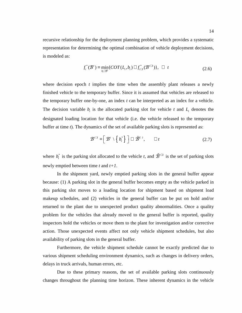
recursive relationship for the deployment planning problem, which provides a systematic

representation for determining the optimal combination of vehicle deployment decisions,

is modeled as:

where decision epoch t implies the time when the assembly plant releases a newly

finished vehicle to the temporary buffer. Since it is assumed that vehicles are released to

the temporary buffer one-by-one, an index t can be interpreted as an index for a vehicle.

The decision variable tb is the allocated parking slot for vehicle t and tL denotes the

designated loading location for that vehicle (i.e. the vehicle released to the temporary

buffer at time t). The dynamics of the set of available parking slots is represented as:

where *tb is the parking slot allocated to the vehicle t, and t 1+B% is the set of parking slots

newly emptied between time t and t+1.

In the shipment yard, newly emptied parking slots in the general buffer appear

because: (1) A parking slot in the general buffer becomes empty as the vehicle parked in

this parking slot moves to a loading location for shipment based on shipment load

makeup schedules, and (2) vehicles in the general buffer can be put on hold and/or

returned to the plant due to unexpected product quality abnormalities. Once a quality

problem for the vehicles that already moved to the general buffer is reported, quality

inspectors hold the vehicles or move them to the plant for investigation and/or corrective

action. Those unexpected events affect not only vehicle shipment schedules, but also

availability of parking slots in the general buffer.

Furthermore, the vehicle shipment schedule cannot be exactly predicted due to

various shipment scheduling environment dynamics, such as changes in delivery orders,

delays in truck arrivals, human errors, etc.

Due to these primary reasons, the set of available parking slots continuously

changes throughout the planning time horizon. These inherent dynamics in the vehicle

* *( ) min{ ( , ) ( )}, t

t

t t 1t t t t 1

bf COT L b f t+

+∈

= + ∀B

B B (2.6)

{ }*\ , t 1 t t 1tb t+ + = ∪ ∀ B B B% (2.7)

15

deployment environment lead consideration of an adaptable and flexible decision-making

approach which can handle the inevitable dynamics.

2.4 Current Best Vehicle Deployment Practice

This section deals with the current best vehicle deployment practice in response to

the dynamic shipment yard environment in the absence of real-time tracking. This

deployment practice is the basis line for validating a new vehicle deployment model with

an RFID-enabled shipment yard and for analyzing the value of RFID technology.

In the current shipment yard, the status of the available parking slots in the

general buffer is periodically updated, perhaps once a day, by a manual reporting process.

Yard operators and truckers manually inform a yard manager of the availability of

parking slots after moving vehicles from the temporary buffer to the general buffer, or

from the general buffer to loading locations. Since this manual reporting and updating

process takes a certain amount of time, immediate updating of the availability of parking

slots in the general buffer is not possible. Figure 2.2 illustrates a vehicle-parking slot

allocation for the current best vehicle deployment practice.

16

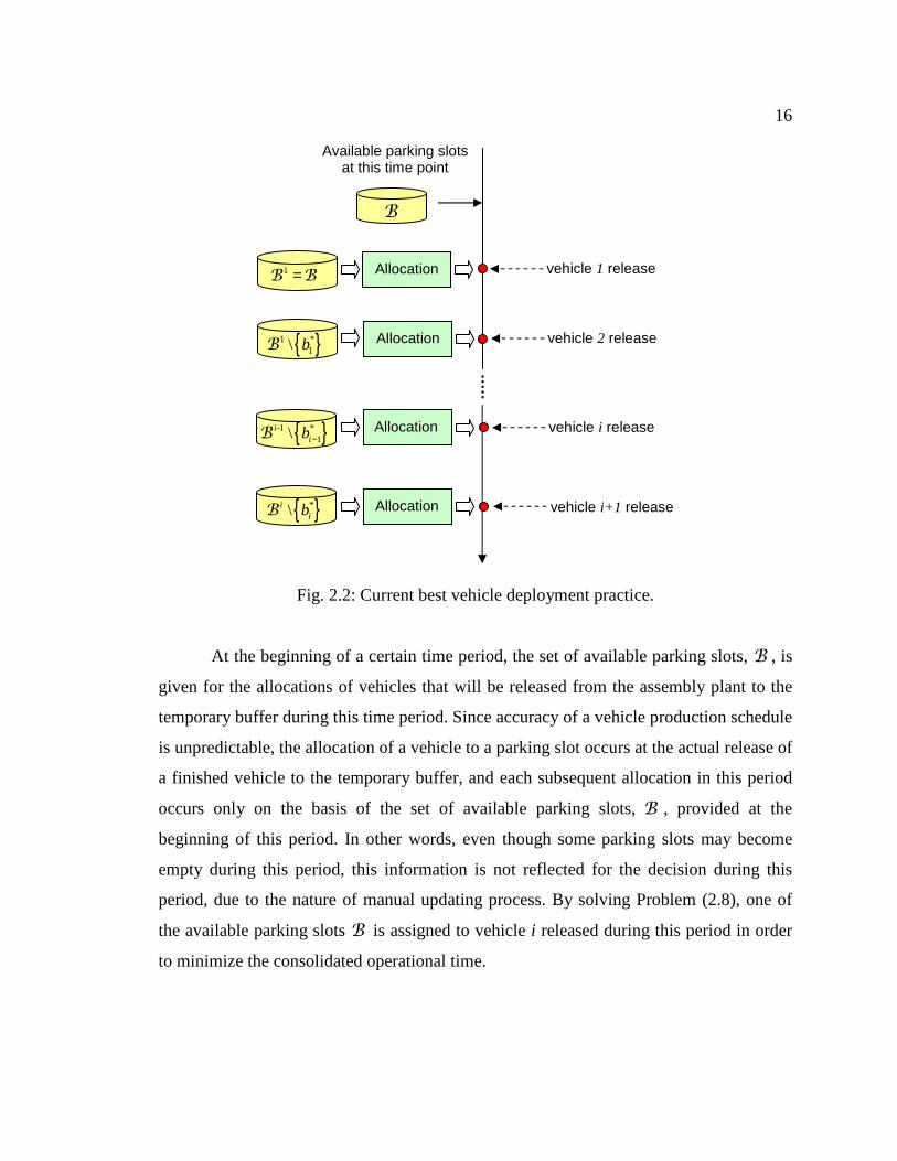
Fig. 2.2: Current best vehicle deployment practice.

At the beginning of a certain time period, the set of available parking slots, B , is

given for the allocations of vehicles that will be released from the assembly plant to the

temporary buffer during this time period. Since accuracy of a vehicle production schedule

is unpredictable, the allocation of a vehicle to a parking slot occurs at the actual release of

a finished vehicle to the temporary buffer, and each subsequent allocation in this period

occurs only on the basis of the set of available parking slots, B , provided at the

beginning of this period. In other words, even though some parking slots may become

empty during this period, this information is not reflected for the decision during this

period, due to the nature of manual updating process. By solving Problem (2.8), one of

the available parking slots B is assigned to vehicle i released during this period in order

to minimize the consolidated operational time.

Available parking slots at this time point

B

vehicle 1 release Allocation

vehicle 2 release

vehicle i release

vehicle i+1 release

Allocation

Allocation { }-1 *1\i

ib −B

Allocation { }*\iibB

{ }1 *1\ bB

1 =B B

17

where binary decision variable ibx is 1 if vehicle i is allocated to parking slot b, ib ∈B ,

otherwise 0. In this formulation, iB , the set of available parking slots for vehicle i, is

obtained from B by excluding iB , i ⊂B B , where iB denotes the set of parking slots

that are already allocated to the vehicles released to the temporary buffer earlier than

vehicle i during this period.

, , , ,

i

d r w i d i iwait load b

b d r w d

D Q b D b Q D L b D b LMin t t x

s s s s∈

+ + + + + ⋅

∑B

subject to

{ }\

, ,

i

ib

b

i i

i ib

x 1

x 0 1 b

∈

=

=∈ ∀ ∈

∑B

B B B

B

(2.8)

18

Chapter 3

Problem II: Shipment Load Makeup - Preliminaries

This chapter details the shipment load makeup process at an automobile

manufacturer by describing the operational environment of shipment load makeup and

providing a mathematical model for shipment load makeup planning. In addition,

dynamic characteristics of the shipment load makeup process are discussed.

3.1 Shipment Load Makeup at Automobile Manufacturer

In an automobile manufacturer’s supply chain, as illustrated in Figure 3.1,

vehicles produced from an assembly plant are temporarily stored at a shipment yard until

they are shipped for delivery. The vehicles in the shipment yard are delivered to

numerous dealers throughout the nation and regional distribution centers via

transportation carriers, such as trucks or trains2 . Typically this activity is labeled

“outbound logistics,” and is an important component of the supply chain.

2 In the case of train transportation, the delivery destinations of vehicles are very limited, and the nature of the shipment load makeup process is relatively straightforward. Thus, this study considers truck transportation only.

19

Fig. 3.1: Supply chains of an automobile manufacturer.

The shipment yard, local dealers, and transportation resource divisions play key

roles in the shipment load makeup process. Thus, a shipment load makeup decision is

made with respect to the different participants’ managerial objectives. Figure 3.2 shows

the key role participants in the shipment load makeup process and their managerial

objectives. The following section discusses the details.

20

Fig. 3.2: Key participants and their managerial objectives in shipment load makeup.

3.2 Specifications of Shipment Load Makeup Environment

3.2.1 Shipment Yard

Everyday, an assembly plant produces thousands of vehicles. Once an assembly

work finishes, the vehicle passes through a required inspection area and proceeds to the

assembly plant’s shipment yard. The vehicle stays in the shipment yard until it is shipped

out via one of the transportation modes, such as a truck or a train

From shipment yard management’s point of view, vehicles in the yard are

considered as inventory, thus, each vehicle creates a holding cost based on its dwell time

in the shipment yard. The dwell time of a vehicle is the amount of time the vehicle stays

in the shipment yard subsequent to its release from the assembly plant. For the purposes

of assuring product quality, the shipment yard sets up a maximum allowed dwell time for

any given vehicle. If the dwell time of a vehicle exceeds this maximum allowable dwell

21

time, the vehicle should be returned to the assembly plant or inspection area to be

overhauled, and this process contributes to additional re-processing costs.

The managerial objective of the shipment yard in the shipment load makeup

process is to minimize total holding and re-processing costs by controlling the amount of

time the vehicles remain in inventory before they are shipped by transportation carriers.

3.2.2 Local Dealer

As explained earlier, the vehicles in the shipment yard are delivered to thousands

of local dealers via trucks. For example, as of December 31, 2006, there were

approximately 7000 General Motors dealers in the United States3. For the shipment load

makeup process, these local dealers are clustered into a number of blocks based on their

geographical adjacency and demand for vehicles, which is shown in Figure 3.3.

Block 1 Block 2

Block n

Dealer 1-1

Dealer 1-2

Dealer 1-3Dealer 1-4

Dealer 1-5

Dealer 2-2

Dealer 2-1

Dealer 2-3

Dealer 2-4

Dealer n-1

Dealer n-2

Dealer n-3

shipment yard

Block 1 Block 2

Block n

Dealer 1-1

Dealer 1-2

Dealer 1-3Dealer 1-4

Dealer 1-5

Dealer 2-2

Dealer 2-1

Dealer 2-3

Dealer 2-4

Dealer n-1

Dealer n-2

Dealer n-3

shipment yard

Fig. 3.3: Local dealers clustered into a number of blocks.

3 http://stocks.us.reuters.com/stocks/fullDescription.asp?symbol=GM&WTmodLOC=C5-Profile-1

22

In automobile manufacturer’s supply chains, an end-customer places an order for

a vehicle with a local dealer directly or through a web-based online system, and receives

the order at the local dealer as soon as the vehicle is ready. To this end, a local dealer

places an order for vehicle(s) with a manufacturer to maintain a profitably safe inventory

level that can meet end-customers’ demands. However, if the vehicle, an end-customer

ordered, is not currently in the inventory of a local dealer, the local dealer places an order

for the vehicle on behalf of the end-customer.

The concept of order-to-delivery (OTD) in automobile manufacturer’s supply

chains is for delivering the vehicles to customers with speed and reliability after

processing the order. The amount of time a vehicle stays at the shipment yard accounts

for large portion of the total OTD lead-time. Thus, reducing the time spent in the

shipment yard is important for achieving the goal of OTD lead-time reduction (Yee et al.,

2007). The managerial objective of a dealer, related to the shipment load makeup process,

is to increase customer fulfillment by reducing OTD lead-time.

3.2.3 Transportation Resource Division

To manage and operate transportation carriers, an automobile manufacturer has its

own transportation resource division or contracts with third party transportation

companies as outsource vendors. From the management perspective of an automobile

manufacturer, these vendors can also be regarded as an internal transportation resource

division.

Transportation carriers such as trucks for delivering vehicles to their destinations

are transportation resources for the shipment load makeup process. Everyday, a number

of trucks arrive sequentially at the shipment yard based on a pre-defined schedule. A

truck takes charge of one of the block areas for delivery of vehicles. This implies that a

truck travels only one block area for delivery of the vehicles ordered from the dealers

located in that block area. Since the dealers located in the same block are geographically

close to each other, it can be reasonably assumed that the traveling sequence of dealers a

truck needs to visit is ignored, and the traveling distance of a truck to a block is regarded

23

as the distance from the shipment yard to the center of the block area. However visiting a

dealer and unloading vehicles at the dealer accrue operational costs whenever a truck

visits a dealer to unload vehicles. For these reasons, the selection of dealers for delivery

affects the utilization of a truck more than just the traveling sequence to dealers.

The managerial objective of the transportation resource division in the shipment

load makeup process is to increase the utilization of a truck by reducing the

corresponding operational costs of delivery, such as traveling cost from the shipment

yard to a block, the total cost for visiting and unloading at dealers, and unutilized truck

capacity cost.

3.2.4 Operational Facts in Shipment Load Makeup

Two operational facts help to describe shipment load makeup operations:

information delay and frequent decision-making environment.

� Information delay: Vehicle information in the shipment yard, including locations

of vehicles, is periodically updated by a manual reporting process. For example,

once a yard operator moves a finished vehicle into the shipment yard, the yard

operator informs the yard manager of the information of the vehicle and its

location. By gathering manually reported information, the yard manager updates

the vehicle information for shipment load makeup. Since the manual reporting

and updating processes take a certain amount of time, the vehicle information is

not updated immediately, but at certain time periods, for example, once a day.

� Frequent decision-making: Everyday a number of trucks arrive sequentially at the

yard to load vehicles. Thus, shipment load makeup decisions for a truck are

required to be made frequently, and each decision should be made in time to

avoid delaying the shipment load makeup operations.

3.3 Shipment Load Makeup Planning

24

From the definition of shipment load makeup given in Chapter 1 and the

understanding of the shipment load makeup environment explained previous sections,

shipment load makeup planning is defined as:

Definition 3.1. (Shipment load makeup planning) The planning for periodic or

sequential shipment load makeup decisions through the planning-time horizon is

shipment load makeup planning. Shipment load makeup planning consists of a set of

shipment load makeup decisions that are decisions for assigning a set of vehicles in the

shipment yard to a set of available spaces on a truck without violating any operational

constraint while achieving the objectives of different functional participants, such as the

shipment yard, local dealers, and the transportation resource division.

3.3.1 Unique Operational Characteristics of Shipment Load Makeup Planning

The unique operational characteristics of shipment load makeup planning are:

� Inevitable dynamics: Because of the dynamics in the market, production, and a

company’s strategy, the schedules of vehicle production and transportation

carrier’s arrival and the managerial objectives of the key participants in shipment

load makeup frequently change. As a result original shipment load makeup plans,

made on the basis of a static environment, are rarely executed as planned, and

dynamic shipment load makeup planning becomes a dominant managerial activity

(Lee, 2002)

� Conflicting objectives from self-interested participants: The aim of shipment load

makeup planning is achieved throughout the functional key participants who are

self-interested for fulfilling their own objectives. These objectives often conflict

with each other. Therefore, a coordination mechanism is necessary to reconcile

the conflicts among the self-interested participants.

� Distributed environment: Since the key participants involved in the shipment load

makeup process are organizationally and/or geographically distributed, local

25

participants can make better decisions for their own objectives with more accurate

and recent information from their local environment.

� Sequential decision-making environment: Because the decisions in the planning

period must be made sequentially, the decisions made in the present may impact

future decisions. Thus, overall long-term effects and expected performance are

consideration throughout the planning period.

3.4 Mathematical Model of Shipment Load Makeup Planning

As defined in the previous section, the set of shipment load makeup decisions for

the planning time period are made together, in advance, with the given schedules of

vehicle production and truck arrival. Shipment load makeup planning is mathematically

formulated using the vehicle information and forecasts of truck availability. The most

common strategy to combine current vehicle information with the forecasted information,

obtained from the schedules of vehicle production and truck arrival, is to use a point

forecast of future events, which produces a rolling horizon procedure. Rolling horizon

procedures have the primary advantages of using classical optimization modeling and

algorithmic technologies. In addition, point forecasts are the easiest for the business

community to understand (Powell et al., 2007). This section, using the rolling horizon

procedure, builds two different mathematical models for different shipment load makeup

planning scenarios in a current shipment yard environment.

3.4.1 Shipment Load Makeup Planning Environment

The shipment load makeup planning environment consists of four main

components: planning time period, set of vehicles, set of trucks, and various costs related

to shipment load makeup.

3.4.1.1 Planning Time Period

26

A shipment load makeup plan, consisting of the set of shipment load makeup

decisions, is made for a certain planning time period. For computational reasons, it is

common to model planning problems of supply chains in discrete time (Wolsey and

Nemhauser, 1999). Thus, the shipment load makeup planning is modeled in discrete time

that can be fixed time periods. Let T be the planning time period represented as a set of

discrete unit time instants.

where endT ( )t T= is the length of the planning horizon. The length of the planning time

horizon is determined based on following information: time period for updating

information of available vehicles in the shipment yard, available truck arrival schedule,

and available vehicle production schedule. Figure 3.4 illustrates the shipment load

makeup planning period in discrete time. In this convention, time beginT ( )t 0= refers to

“here and now,” while discrete time period t refers to the time interval between t-1 and t.

Fig. 3.4: Shipment load makeup planning time period.

{ }, , , , , ,begin endT T 0 1 2 T 1 T = = − T L (3.1)

Planning time period

Tbegin (t=0) Tend (t=T)

Vehicle production schedule

Truck arrival schedule

Build shipment load makeup plan

at t=0

27

This modeling of the planning time period views information as arriving

continuously over time, while a shipment load makeup decision will be made at a discrete

time point. Since the decisions in the shipment load makeup planning are made at

discrete time point, information required to support making the decisions, such as state

variables and cost functions, are also represented in discrete time.

3.4.1.2 Set of Vehicles

The set of vehicles available for shipment load makeup planning is represented as:

in which, 0V denotes the set of vehicles in the shipment yard at time t=0 (where

shipment load makeup plan is made), and [ ],P0 TV is the set of vehicles scheduled to be

produced during the given planning time period.

A vehicle v, v ∈V , has the following attributes that support shipment load

makeup planning.

� vb : A block index of vehicle v, vb ∈B , where B is the set of blocks.

� vd : A dealer index of vehicle v, vd ∈D , where D is the set of dealers.

� vω : A shipment time commitment for vehicle v. This attribute represents an order

priority.

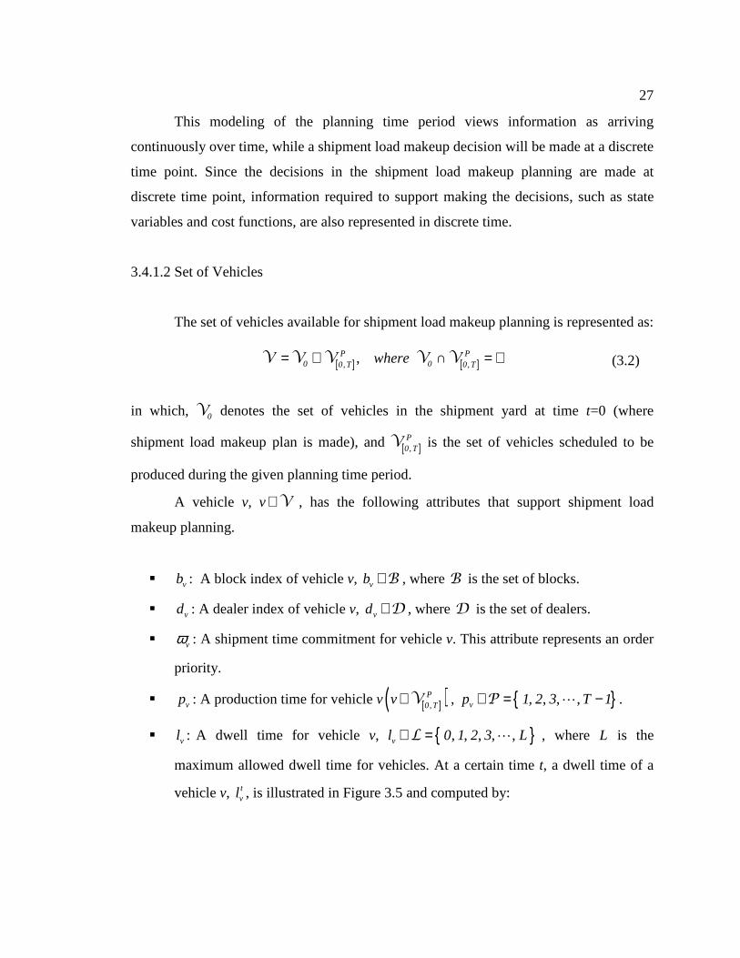
� vp : A production time for vehicle v [ ]( ),P0 Tv ∈V , { }, , , ,vp 1 2 3 T 1∈ = −P L .

� vl : A dwell time for vehicle v, { }, , , , ,vl 0 1 2 3 L∈ =L L , where L is the

maximum allowed dwell time for vehicles. At a certain time t, a dwell time of a

vehicle v, tvl , is illustrated in Figure 3.5 and computed by:

[ ] [ ], ,,P P0 00 T 0 Twhere= ∪ ∩ = ∅V V V V V (3.2)

28

[ ],

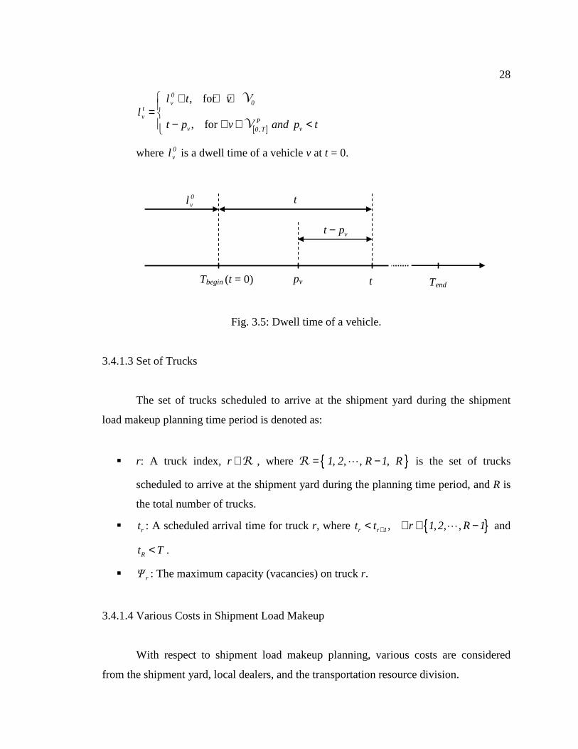
, for

, for

0v 0

tv

Pv v0 T

l t vl

t p v and p t

+ ∀ ∈=

− ∀ ∈ <

V

V

where 0vl is a dwell time of a vehicle v at t = 0.

Fig. 3.5: Dwell time of a vehicle.

3.4.1.3 Set of Trucks

The set of trucks scheduled to arrive at the shipment yard during the shipment

load makeup planning time period is denoted as:

� r: A truck index, r ∈R , where { }, , , ,1 2 R 1 R= −R L is the set of trucks

scheduled to arrive at the shipment yard during the planning time period, and R is

the total number of trucks.

� rt : A scheduled arrival time for truck r, where { }, , , ,r r 1t t r 1 2 R 1+< ∀ ∈ −L and

Rt T< .

� rΨ : The maximum capacity (vacancies) on truck r.

3.4.1.4 Various Costs in Shipment Load Makeup

With respect to shipment load makeup planning, various costs are considered

from the shipment yard, local dealers, and the transportation resource division.

Tbegin (t = 0) t pv Tend

0vl

vt p−

t

29

From the shipment yard’s point of view, following two costs are considered.

� ( )hdc l : Vehicle holding cost during time period [l-1, l], represented as a

monotonically increasing function.

� [ ] ( ),1 2

HDt tC v : Holding cost for vehicle v during time period, [t1, t2], computed by:

[ ] ( ) ( )( )

,

t1v 2 1

1 2t1v

l t tHD hdt t

l l 1

C v c l+ −

= +

= ∑

� rpc : Re-processing cost (i.e. extra treatment cost) for over-dwelled vehicle.

� [ ] ( ),1 2

RPt tC v : Re-processing cost for vehicle v during time period, [t1, t2], computed

by:

[ ] ( )( )

,

, if ,

, otherwise

1

1 2

trpv 2 1RP

t t

c l L t t 1 LC v

0

∈ − − + =

The vehicle holding cost and the re-processing cost are combined as shown in

Figure 3.6(a), and Figure 3.6(b) illustrates a cumulative holding cost for a vehicle as

dwell time increases.

Fig. 3.6: Costs in shipment yard.

From the local dealers’ point of view, following customer fulfillment related costs

are considered.

L 0

cost

rpc

( )hdc l

(a)

dwell time ( l ) L 0

cost

(b)

dwell time ( l )

30

� ( )dlvc l : Order delay cost for vehicle v during time period, [l-1, l], represented as a

monotonically increasing function.

� [ ] ( ),1 2

DLt tC v : Order delay cost for vehicle v during time period, [t1, t2], computed by:

[ ] ( ) ( )( )

,

t1v 2 1

1 2t1v

l t tDL dl

vt tl l 1

C v c l+ −

= +

= ∑

� ltvc : Lost order cost for vehicle v.

� [ ] ( ),1 2

LTt tC v : Lost order cost for vehicle v during time period, [t1, t2], computed by:

[ ] ( )( )

,

, if ,

, otherwise

1

1 2

tltv v 2 1LT

t t

c l L t t 1 LC v

0

∈ − − + =

The order delay cost and the lost order cost for vehicle v are combined as shown

in Figure 3.7(a), and Figure 3.7(b) illustrates a cumulative order delay cost for vehicle v .

Fig. 3.7: Costs for vehicle v in local dealer vd .

In the above figures, vω denotes a commitment to an order shipment time for

vehicle v to dealer vd , where { }|v v v vand Lω ω ω ω∈ ∈ <L .

L 0

cost

ltvc

( )dlvc l

(a)

dwell time ( l ) L 0

cost

(b)

dwell time ( l ) vω vω

31

For the transportation resource division, truck utilization related costs are

considered.

� TRrbC : Traveling cost of truck r from the shipment yard to block b.

� ULrbdC : Visiting and unloading cost of truck r at dealer d in block b.

� URrC : Unutilized capacity cost per vacancy for truck r.

3.4.2 Integer Programming Models for Two Different Scenarios

This section builds the mathematical models for two different shipment load makeup

scenarios in a current shipment yard environment. According to divisibility of vehicles

involved in the same dealer, two different shipment load makeup scenarios are defined

as:

� Scenario 1: The vehicles involved in the same dealer are indivisible through

shipment load makeup planning.

� Scenario 2: The vehicles involved in the same dealer can be divisible through

shipment load makeup planning.

The mathematical models for scenario 1 and 2 are formulated in Sections 3.4.2.1

and 3.4.2.2, respectively.

3.4.2.1 Scenario 1: Vehicles are Indivisible

3.4.2.1.1 Decision Variables

The two binary decision variables for the shipment load makeup planning are

defined as:

32

, if truck is assigned to block for delivering vehicles

, otherwise

rb

1 r b

0δ

=

, if vehicles of dealer in block chosen for shipment by truck

, otherwise

rbd

1 d b rx

0

=

3.4.2.1.2 Objective Function of Shipment Load Makeup Planning

The objective function of the shipment load makeup planning is an integrated

framework for simultaneously optimizing three sub-objective functions, which are for the

shipment yard, local dealers, and the transportation resource division, respectively. Each

sub-objective function computes the shipment load makeup related cost. Thus, the goal of

shipment load makeup planning is for minimizing the total shipment load makeup cost,

and the objective function, required to be minimized, is stated as:

where, ( )rS bdF x , ( )r

D bdF x and ( ),r rT b bdF xδ denote objective functions of the shipment

yard, local dealers, and the transportation resource division, respectively.

A. Objective Function of Shipment Yard: ( )rS bdF x

Based on understanding the managerial objective for the shipment yard in

shipment load makeup planning, explained in Section 3.2.1, the objective function of the

shipment yard is mathematically formulated as:

( ) ( ) ( ) ( ),r r r r rbd S bd D bd T b bdF x F x F x F xδ= + + (3.3)

33

In the above objective function, r

bdtV denotes the set of available vehicles for

dealer d in bock b when truck r arrives at the shipment yard and R 1t + implies T.

B. Objective Function of Local Dealers: ( )rD bdF x

As described in Section 3.2.2, the managerial objective of local dealers is to

enhance customer fulfillment by reducing OTD lead time. Now the objective function for

local dealers is designed as:

C. Objective Function of Transportation Resource Division: ( ),r rT b bdF xδ

( ) ( ) [ ] ( ) [ ] ( )

[ ] ( ) ( )( ){ }

[ ] ( )( )

, ,

min ,

,

,

,

, if ,

, otherwise

r r 1 r r 1bd

b tr

trv r 1 r

r r 1trv

r

r r 1

r r HD RPS bd bd t t t t

r b d v

l t t L

HD hdt t

l l 1

trpv r 1 rRP

t t

F x 1 x C v C v

where C v c l

c l L t t 1 LC v

0

+ +

+

+

+

∈ ∈ ∈ ∈

+ −

= +

+

= − ⋅ +

=

∈ − − + =

∑∑ ∑ ∑

∑

R B D V

(3.4)

( ) ( ) [ ] ( ) [ ] ( )

[ ] ( ) ( )( ){ }

( )

, ,

min ,

,

, if ,

, otherwise

r r 1 r r 1bd

b tr

trv r 1 r

r

vr r 1

r r DL LTD bd bd t t t t

r b d v

l t t L

tdlv v v r 1 rDL

l 1t t

F x 1 x C v C v

c l l t t 1 L 1where C v

0

ωω

+ +

+

+

∈ ∈ ∈ ∈

+ −

+= +

= − ⋅ +

∈ − − + − =

∑∑ ∑ ∑

∑

R B D V

[ ] ( )( )

,

, if ,

, otherwise

r

r r 1

tltv v r 1 rLT

t t

c l L t t 1 LC v

0+

+ ∈ − − + =

(3.5)

34

The objective function of the transportation division is the sum of the shipment

load makeup related costs, such as traveling cost, visiting and unloading cost, and an

unutilized truck capacity cost:

3.4.2.1.3 Integer Programming Formulation for Scenario 1

This study formulates the shipment load makeup planning for minimizing the sum

of the planning related costs through an Integer Programming (IP) model. As shown in

the following formulation, the number of variables increases rapidly according to the

increase in the planning time horizon, the number of blocks, the number of dealers in

each block, and the number of trucks. This formulation is basically a centralized

decision-making formulation, and it may not directly apply to shipment load makeup

planning in a real shipment yard environment. Instead this formulation serves the

purposes of value analysis of introducing RFID in the shipment yard.

As explained in Section 3.4.2.1.2, the objective function consists of three sub-

objective functions. In Equation (3.7), sub-objective function ( )rS bdF x represents the sum

of total holding and re-processing costs incurred during the planning period, ( )rD bdF x

represents the sum of total order delay and lost order costs incurred during the planning

period, and ( )rT bdF x represents the sum of total traveling, visiting and unloading, and

unutilized capacity costs. In the IP formulation, constraint (3.8) ensures a single truck can

take charge of only one block area for the delivery. Constraint (3.9) presents all the local

dealers selected for delivery by a certain truck must be included in the same block. In this

equation, M is an extremely large positive number that exceeds the maximum feasible

( ),

b

r

b

r r r TR r ULT b bd b rb bd rbd

r b r b d

r bd URr bd t r

r b d

F x C x C

x C

δ δ

Ψ

∈ ∈ ∈ ∈ ∈

∈ ∈ ∈

= ⋅ + ⋅

+ − ⋅ ⋅

∑∑ ∑∑ ∑

∑ ∑ ∑

R B R B D

R B D

V

(3.6)

35

value of anyb

rbd

d

x∈∑D

( ),r b∀ ∈ ∈R B . Constraint (3.10) ensures the number of vehicles

loaded onto a truck can not exceed the maximum capacity of the truck, where r

bdtV is the

set of vehicles ordered from the dealer d in block b and available when truck r arrives.

Equation (3.11) represents the dynamics of the set of available vehicles in the shipment

yard. In this equation, ( ),1 2

Et tV represents the set of vehicles that become unavailable for

the delivery during time period, [t1, t2], due to maximum allowed dwell time, ( ),1 2

Pt tV

denotes the set of vehicles produced during the time period, [t1, t2], and SrV is the set of

vehicles loaded onto truck r for delivery.

subject to:

( ) ( ) ( ) ( ),r r r r rbd S bd D bd T b bdMinimize F x = F x F x F xδ+ + (3.7)

,rb

b

1 rδ∈

= ∀ ∈∑B

R (3.8)

, ,b

r rbd b

d

x M 0 r bδ∈

− ⋅ ≤ ∀ ∈ ∈∑D

R B (3.9)

,r

b

r bdbd t r

b d

x Ψ r∈ ∈

⋅ ≤ ∀ ∈∑ ∑B D

V R (3.10)

[ ] [ ]

[ ]{ } [ ] { }

, ,

- , ,

\ , for

\ , for , , ,

r r

r

r 1 r 1 r r 1 r

E P0 0 t 0 t

tS E P

t r 1 t t t t

r 1

r 2 R 1 R− − −

∪ =

= ∪ ∪ ∀ ∈ −

V V V

V

V V V V L

(3.11)

{ }, , ,rb 0 1 r bδ ∈ ∀ ∈ ∈R B

{ }, , , ,rbd bx 0 1 r b d∈ ∀ ∈ ∈ ∈R B D

36

3.4.2.2 Scenario 2: Vehicles are Divisible

3.4.2.2.1 Decision Variables

The three binary decision variables for the shipment load makeup planning are

defined as:


, otherwise

rb

1 r b

0δ

=

, if truck visits dealer in block for delivering vehicle

, otherwise

rbd

1 r d b

0µ

=

, if vehicle is chosen for shipment by truck

, otherwise

rv

1 v rx

0

=

3.4.2.2.2 Objective Function of Shipment Load Makeup Planning

The objective function, required to be minimized, is stated as:

where, ( )rS vF x , ( )r

D vF x , and ( ), ,r r rT b bd vF xδ µ , denote objective functions of the shipment

yard, local dealers, and the transportation resource division, respectively.

A. Objective Function of Shipment Yard: ( )rS vF x

where rt

V denotes the set of available vehicles when truck r arrives at the shipment yard

and R 1t + implies T.

( ) ( ) ( ) ( ), ,r r r r r rv S v D v T b bd vF x F x F x F xδ µ= + + (3.12)

( ) ( ) [ ] ( ) [ ] ( ), ,r r 1 r r 1

tr

r r HD RPS v v t t t t

r v

F x 1 x C v C v+ +

∈ ∈

= − ⋅ + ∑ ∑

R V

(3.13)

37

B. Objective Function of Local Dealers: ( )rD vF x

C. Objective Function of Transportation Resource Division: ( ), ,r r rT b bd vF xδ µ

3.4.2.2.3 Integer Programming Formulation for Scenario 2

This section formulates the shipment load makeup planning, where the vehicles

ordered from the same local dealer can be divisible. As shown in the following

formulation, the number of variables increases significantly according to the increase of

the planning time horizon, the number of vehicles, the number of blocks, the number of

dealers in each block, and the number of trucks, and it may not directly apply to a real

shipment yard environment.

In the IP formulation, constraint (3.17) ensures that a single truck can take charge

of only one block area for the delivery. Constraint (3.18) presents all the vehicles selected

for delivery by a certain truck must be included in the same block, where r

btV is the set of

vehicles ordered from the local dealers in block b and available when truck r arrives at

the shipment yard. In this equation, M1 is an extremely large positive number that

exceeds the maximum feasible value of anyb

tr

rv

v

x∈∑V

( ),r b∀ ∈ ∈R B . Constraint (3.19)

determines that a truck should visit a dealer if any vehicle ordered by the dealer is loaded

onto the truck, where r

bdtV is the set of vehicles ordered by the dealer d in block b and

available when truck r arrives. As explained in Constraint (3.18), M2 is an extremely

( ) ( ) [ ] ( ) [ ] ( ), ,r r 1 r r 1

tr

r r DL LTD v v t t t t

r v

F x 1 x C v C v+ +

∈ ∈

= − ⋅ + ∑ ∑

R V

(3.14)

( ), ,

b

tr

r r r r TR r ULT b bd v b rb bd rbd

r b r b d

r URr v r

r v

F x C C

x C

δ µ δ µ

Ψ

∈ ∈ ∈ ∈ ∈

∈ ∈

= ⋅ + ⋅

+ − ⋅

∑∑ ∑∑ ∑

∑ ∑

R B R B D

R V

(3.15)

38

large positive number that exceeds the maximum feasible value of anybd

tr

rv

v

x∈∑V

( ), , br b d∀ ∈ ∈ ∈R B D . Constraint (3.20) ensures the number of vehicles loaded onto

a truck can not exceed the maximum capacity of the truck. Equation (3.21) represents the

dynamics of the set of available vehicles.

subject to:

( ) ( ) ( ) ( ), ,r r r r r rv S v D v T b bd vMinimize F x = F x F x F xδ µ+ + (3.16)

,rb

b

1 rδ∈

= ∀ ∈∑B

R (3.17)

, ,b

tr

r rv 1 b

v

x M 0 r bδ∈

− ⋅ ≤ ∀ ∈ ∈∑V

R B (3.18)

, , ,bd

tr

r rv 2 bd b

v

x M 0 r b dµ∈

− ⋅ ≤ ∀ ∈ ∈ ∈∑V

R B D (3.19)

,tr

rv r

v

x Ψ r∈

≤ ∀ ∈∑V

R (3.20)

[ ] [ ]

[ ]{ } [ ] { }

, ,

- , ,

\ , for

\ , for , , ,

r r

r

r 1 r 1 r r 1 r

E P0 0 t 0 t

tS E P

t r 1 t t t t

r 1

r 2 R 1 R− − −

∪ =

= ∪ ∪ ∀ ∈ −

V V V

V

V V V V L

(3.21)

{ }, , ,rb 0 1 r bδ ∈ ∀ ∈ ∈R B

{ }, , , ,rbd b0 1 r b dµ ∈ ∀ ∈ ∈ ∈R B D

{ }, , ,rvx 0 1 r v∈ ∀ ∈ ∈R V

39

3.5 Computational Complexity and Limitations in Real Environment

This section discusses the computational complexity of the shipment load makeup

planning models and presents limitations to a real shipment yard environment in applying

these models, which are formulated as a centralized decision-making process.

3.5.1 Computational Complexity of Shipment Load Makeup Planning

The shipment load makeup planning formulated in Section 3.4.2 is a problem of

deterministic sequential decision-making. Florian et al. (1980) investigate the

computational complexity of deterministic sequential decision-making problems and

established NP-hardness for such problems.

Dynamic programming (DP), originally proposed by Bellman (1957), has been a

useful mathematical technique for making a sequence of interrelated decisions and

provides a systematic procedure for determining the optimal combination of decisions

(Hiller and Lieberman, 1995). All applications of DP, however, have the restriction of

“curse of dimensionality,” i.e. the extremely fast growth of solution space (and

computational time), as the problem size increases (Steiner, 1990). In order to show the

curse of dimensionality, even in the simplified case4 in which only one block area exists,

investigation of the number of feasible solutions which may represent the solution space

for the IP model is conducted. The number of feasible solutions for a simplified case of

shipment load makeup planning is computed by:

4 Since the shipment load makeup planning where the vehicles can be divisible (Scenario 1) is more general scenario, we investigate the curse of dimensionality for this scenario.

( ) ( ) ( )! ! !

! ! ! ! ! !

1 2 R

1 2 R

1 2 R

t t t

1 2 R

t t t

1 t 1 2 t 2 R t R

Ψ Ψ Ψ

Ψ Ψ Ψ Ψ Ψ Ψ

× × ×

= × × ×⋅ − ⋅ − ⋅ −

V V V

V V V

V V V

L

L

(3.22)

40

where rt

V is the number of available vehicles when truck r arrives. For example, the

solution space of the small size shipment load makeup planning,

where { } and , , ,rt r15 5 r 1 2 3Ψ= = ∀ ∈ =V R , is obtained as:

For a simplified case of shipment load makeup planning, Figures 3.8 and 3.9

show the extremely fast growth of the solution space as the average number of available

vehicles when a truck arrives increases and as the number of trucks increases,

respectively. In Figure 3.8 the number of trucks R and the maximum capacity of each

truck rΨ are set to 3 and 4, respectively, and the average number of available vehicles

rtV and the maximum capacity of each truck rΨ are set to 8 and 4, respectively, in

Figure 3.9.

Fig. 3.8: The growth of solution space as the average number of vehicles rt

V increases

( { }, ,1 2 3=R and ,r 4 rΨ = ∀ ∈R ).

( )!

.! !

3 3

1015 15

2 708 105 15 55

= ≈ × ⋅ −

(3.23)

0

1000000

2000000

3000000

4000000

5000000

6000000

7000000

8000000

9000000

10000000

5 6 7 8 9 10

125 3375 42875 343000

200376

9261000

rtVThe average number of vehicles when a truck arrives:

41

Fig. 3.9: The growth of solution space as the number trucks R increases (rt

8=V and

,r 4 rΨ = ∀ ∈R ).

In addition to the curse of dimensionality, the mathematical model of shipment

load makeup planning, where the vehicles ordered from the same dealer are not divisible

(Scenario 1), is NP-complete.

Proposition: Shipment load makeup where the vehicles are not divisible (Scenario 1) is

NP-complete:

Consider a 0/1 knapsack problem with item j ∈ J , { }, , , ,1 2 3 JJ = L where J is the

total number of items. Each item j has a profit jp and weight jw and the total weight (or

capacity) of a knapsack is C. The 0/1 knapsack problem can be generally formulated as:

J

j jj 1

Maximize p x=

⋅∑

subject to: J

j jj 1

w x C=

⋅ ≤∑

{ }, ,jx 0 1 j∈ ∀ ∈ J

0

2E+10

4E+10

6E+10

8E+10

1E+11

1.2E+11

1.4E+11

1 2 3 4 5 6

70 4900 343000 2.40E+07 1.68E+09

1.18E+11

The number of trucks arriving during the planning period: R

42

Proof: Consider a very simplified version of shipment load makeup planning problem,

where only one truck and one block area are considered, while the objective function of

transportation resource division is ignored. Then truck index r, block index b, binary

decision variable rbδ , and constraints (3.8), (3.9) and (3.11) can be removed from the

mathematical formulation provided in Section 3.4.2.1.3. Since only one truck and one

block area are considered, now the original binary decision variable, rbdx , can be

simplified as jx , where index j represents a local dealer. Now the corresponding

formulation is:

( ) ( ) ( ) ( )j j

HD RP DL LTj

v v

C v C v C v C v p∈ ∈

+ + + = ∑ ∑V V

jjw=V

Ψ C=

From the above formulation, it is clear that the simplified version of shipment load

makeup planning problem is formulated as a 0/1 knapsack problem.

Since the 0/1 knapsack problem is known as NP-complete, by induction the

shipment load makeup planning problem where the vehicles are not divisible (Scenario 1)

is also NP-complete . �

3.5.2 Limitations in a Real Shipment Yard Environment

Shipment load makeup planning is formulated on the basis of centralized

information processing and decision-making, where a decision maker should have all

business and operational information for numerous local dealers and the transportation

resource division. In the supply chains of an automobile manufacturer, this business and

43

operational information changes frequently as business strategies and environments of

local dealers and the transportation resource division change.

In this centralized shipment load makeup planning the decision maker should be

aware of all the vehicle information in the shipment yard. However, the set of available

vehicles in the shipment yard, when a shipment load makeup plan is made, can change

throughout the planning period. For example, vehicles in the shipment yard can be put on

hold and/or returned to the assembly plant or the inspection area due to unexpected

product quality abnormalities. For that reason, a vehicle, planned to be loaded onto a

certain truck, can be unavailable for the delivery when the truck actually arrives at the

shipment yard.

Furthermore shipment load makeup planning formulation assumes that the

decision maker receives 100% accurate vehicle production and truck arrival schedules for

the planning time period when the plan is made at the beginning of the planning period.

For that reason, possibly, the shipment load makeup plan could recommend loading a

vehicle that has been scheduled but has not really been produced or, loading the set of

vehicles onto a truck that has been scheduled but has not really arrived on time.

As dynamics and uncertainties in the shipment load makeup planning

environment increase, the centralized decision-making approach becomes inadequate in

processing all the distributed information from the shipment yard, local dealers, and the

transportation division. These dynamics create an inability to provide adaptable plans in

response to uncertain vehicle production and truck arrival schedules. Moreover, even

assuming that the decision maker has all the distributed information and precisely

forecasted schedules, applying shipment load makeup planning model directly to large

scale real shipment load makeup environments is practically and computationally

unsuitable.

44

Chapter 4

Background Literature Survey

As discussed in Chapter 1, the main objective of this study is to develop

decentralized decision-making approaches for the vehicle deployment and the shipment

load makeup in an RFID-enabled shipment yard environment. This chapter reviews some

background literature which is related to the current problem domains and

methodologies, such as RFID-enabled applications, management of shipment yard in an

automobile industry, and market-based control mechanism.

4.1 RFID-enabled Applications

An RFID is one type of wireless automatic identification technology that uses

radio waves to identify the location and the presence of an individual physical object

when the object is in a readable range. Two primary components of RFID applications

are RF tags and the RFID reader. An RF tag consists of a microchip and an antenna. The

microchip stores information of object such as a unique identification number. The

antenna in an RF tag enables the microchip to transmit information of object to an RFID

reader, which communicate with RF tags and transforms the information on the RF tag to

a format understandable by application hosts (Angeles, 2005).

This emerging technology is able to identify and detect the location and the

presence of an object in an automated and timely manner when the object is in a readable

range. By virtue of these abilities, the RFID-enabled systems promise to provide near-

perfect information visibility throughout the business process by tracking all the entities,

including resources and finished products, and allowing instant identification and

automatic information transfer of the entities’ status. Providing real-time information

visibility and the status of business entities may bring up new opportunities to improve

45

business efficiency and value addition (Datta and Viguier, 2000; Hanebeck and Tracey,

2003; Walker, 2005).

4.1.1 RFID in Various Business Areas

In recent years, RFID technologies have been widely introduced into various real-

world business environments, such as retail, agriculture, healthcare, transportation

service, construction, supply chains, etc., and several companies are investigating how

RFID can be used for improving their business performance and how it can help in value

addition for them.

Kourouthanassis and Roussos (2003) and Jones et al. (2005) discuss the

implementation and impact of an RFID-enabled retail system. The adoption of RFID

technologies enhances structural integration within the retail sector of the economy and

provides wide range of benefits throughout retail operations at shop floor level and the

customers’ shopping experience.

Watts et al. (2002) present a need for automatic identification and data transfer in

agricultural environment where the incorrect application of chemicals could have

significant environmental impacts, and Ng et al. (2005) and Trevarthen (2007) present

how RFID technologies can be utilized on the livestock farming industry where livestock

is required to be controlled and tracked for disease control, breeding management, and

stock management.

As RFID-enabled applications in the healthcare area, Li et al. (2004), Wang et al.

(2006), Ho et al. (2005) introduce a mobile healthcare service system that adopts RFID

technologies for tracking and identifying patients and objects for inside and outside

hospital. This RFID-enabled mobile healthcare service system has the potential to

contribute to hospital operating efficiency, good medical service and patient safety. This

study also demonstrates how an RFID-enabled healthcare system enables hospital and

government to effectively conduct real-time infection control.

Blythe (1999) provides an insight into the use of RFID technologies to facilitate

roadside to vehicle data communications for automatic tolling and road use pricing

46

systems. This study also discusses RFID technologies have potentials to allow a high

performance road to vehicle two way communications which can offer value added

services, such as driver information and trip planning, parking reservation and payment,

dynamic route guidance, and vehicle monitoring. Cerino and Walsh (2000) and Legner

and Thiesse (2006) present implementation of RFID prototype systems to support

integrated facility management processes in the aviation industry.

For the construction area Moy (2007) and Jaselskis et al. (1995) discuss how

RFID technologies can help construction and property organizations to manage assets,

workforces, and operations more effectively and to optimize the use of property portfolio

and associated real estate assets effectively.

Due to a result of global competition, the automobile industry has always held a

leading position in the adoption of new technologies to improve their processes and

products. Srinivasan et al. (1994) argue that accurate, frequent, and timely exchange of

information enables higher information integration between an assembly plant and its

suppliers in supply chains of the automobile industry. This study provides empirical

evidence that the information integration enhances shipment performance of suppliers in

a Just-in-Time environment of the automobile industry. Strassner and Fleisch (2003) and

Strassner et al. (2005) discuss RFID technologies utilized in a wide range of applications

in the automobile industry, including container tracking, work-in-progress tracking,

vehicle identification and access control, etc.

4.1.2 RFID in Supply Chains

The adoption of RFID technologies is especially prevalent within management of

supply chains where limitations exist due to the inaccuracies and delays of product

identification throughout the product life cycle (McFarlane et al., 2003; Saygin, 2007).

A supply chain is defined as a network of all of functional stages and

organizations involved in fulfilling a customer request. The functions involved in filling a

customer request include development of new product, procurement of materials,

transformation of the materials into finished products, distribution of the finished

47

products, finance, marketing, and customer service (Ganeshan and Harrison, 1995;

Chopra and Meindl, 2001).

The RFID technologies hold the promise of closing the information gaps in the

supply chains, and these new technologies are effectively adopted in various functional

operations in supply chains, such inventory control, resource management, shipment

operation, warehouse management, recycling and disposal management etc.

Saygin (2007) presents RFID-enabled inventory management models for time

sensitive materials on a shop floor. Using the simulation studies, the impact of integrating

RFID technologies with inventory control is analyzed. The experiment results show that

the RFID-enabled inventory model can effectively adapt to dynamics in shop floor

inventory control environment. In this study Saygin (2007) emphasize a need for RFID-

enabled effective decision-making algorithms that can lead benefits in introducing RFID

technologies.

Ford Motor Co.’s facility in Mexico has adopted RFID for automatic and real-

time identification of auto and truck parts as they went through the plant floor production

line (Johnson, 2002). In this RFID-enabled production line, an RF tag attached on a part

includes information of specific operations that need to be done at each station. By

enabling updates or changes in operational information to be recorded to the RF tag,

operational processes in the production line are constantly being updated without risk of

operator error.

Angeles (2005) illustrates the significant potential of the RFID technology in

logistics operations. A specific RFID technology implementation is described to

demonstrate the benefits being realized with the RFID technology. Chow et al. (2006)

present the RFID-enabled resource management system where the case-based reasoning

technology is integrated to improve warehouse operating performance by tracking and

optimizing resource (material handling equipments) utilization. Liu et al. (2006) discuss

RFID-enabled resource management system. The results of this study show that the RFID

technology enhances the performance of warehouse operations by increasing rack space

utilization and loading speed and decreasing work-related errors and operational costs.

48

Kim et al. (2005) examine the feasibility of adopting RFID technology to enhance

the efficiency and productivity of two major operations in container terminals, such as the

gate and storage operations. The results of this study imply that the real-time information

of containers provided by the RFID system enables terminal operators to plan the gate

and storage operations more efficiently by reducing the operational processing time and

re-handling work and improving the reliability of container information. Park et al.

(2006) propose RFID-enabled real-time location system (RTLS) to improve the

performance of container terminal operation system. This study suggests that the RFID-

enabled RTLS system enables the effective planning of container loading sequence. In

addition, the RFID system can support operations of gantry cranes and yard tractors, and

shorten ship turnaround time, more efficiently. Finally it can accomplish the reduction of

whole lead-time of port logistics.

The lack of lifecycle information about returned products is known as a major

obstacle to efficient product recovery and disposal management. Kulkarni et al. (2005)

examines the benefits of networked RFID systems which can allow automatically

tracking and transferring item level product information. These benefits enable to

improve decisions and processes occurred in product recovery and disposal stages.

4.2 Management of Automobile Shipment Yard

In the United States, non-military logistics costs are estimated to be over 11% of

the Gross National Product (GNP) and constitute about 30% of the cost of the products

sold (Thomas and Griffin, 1996). Hence the coordination of logistics operations and the

design of effective distribution models have been extensively studied for various industry

areas.

The outbound logistics for finished vehicles has grown significantly during the

last decade, and the oligopolistic structure of the market has led to an impressive increase

in competition among the vehicle transshipment hubs, such as shipment yard, vehicle

distribution centers or port. Thus, the management of a transshipment hub is one of the

most important activities in outbound logistics of an automobile industry. To survive

49

from this competitive environment, management of a vehicle transshipment hub must

meet to highly demanded and dynamic market environment and provide reliable service

while enhancing managerial or operational efficiency (Mattfeld and Kopfer, 2003).

The managerial or operational decision-making models related to vehicle

transshipment hub of automobile industry can depend on methodological support offered

by general approaches for decision-making models in hub management, such as facility

location and layout (Domschke and Krispin, 1997; Owen and Daskin, 1998; Klose and

Drexl, 2005), routing, scheduling, and planning (Hariga and Jackson, 1996; Berg, 1999;

Vis and Koster, 2003; Christiansen et al., 2004), the design of storage space allocation

(Iranpour and Tung, 1989; Cassady and Kobza, 1998; Kim and Park, 2003; Gue, 2006),

and shipment loading issues (Agbegha et al., 1998; Nishimura et al., 2001; Tadei et al.,

2002; Attanasio et al., 2007). However there are limited literatures which directly address

the management or operational decision-making models in a shipment yard of an

automobile manufacturer.

Mattfeld and Kopfer (2003) report on the development of an automated planning

and scheduling system intended to support operations for the transportation of finished

vehicles in a transshipment hub. They address current terminal operational processes and

model an integral decision-making problem for manpower planning and inventory control

in a vehicle transshipment hub. In order to alleviate the complexity of the decision-

making problem, they develop a two-stage hierarchical decision-making problem. In the

iterative decision support framework, the heuristic solution procedures are proposed to

solve the decomposed sub-stage problems.

Mattfeld and Orth (2006) address the planning model of transportation and

storage capacity in a vehicle intermodal transshipment terminal, which consists of

spatially distributed storage areas of limited capacity interconnected by travel ways. In

order to improve the operational efficiency of the vehicle transshipment terminal, they

develop the optimization model of the multi-period-capacitated storage space allocation

problem. The evolutionary algorithm developed in this study evolves a period-oriented

capacity utilization strategy. This capacity utilization strategy controls a construction

50

heuristic (greedy approach) which efficiently assigns vehicle movements to periods and

vehicles to storage locations.

Eskigun (2002) and Howard et al. (2005) address an important development in the

automobile industry in recent years has been an increased interest in reducing the lead-

time required to deliver finished vehicles from the assembly plants to local dealers or the

customer, and the lead-time significantly influences the distribution costs and the make-

to-order policy that most automakers try to achieve.

Jin et al. (2007) study an automobile distribution network with a strategic

transportation mode selection. Because transportation lead-time influences the turnaround

rate of transportation mode and shipment volume largely impacts on the total lead-time,

the study addresses quantity discount model for transportation cost structures. In the

strategic decision-making point of view, this study proposes a management strategy

based on Integer Programming (IP) model to minimize the total distribution costs by

making a transportation mode selection decision.

Eskigun (2002) and Eskigun et al. (2005) propose a large-scale network design

model for the outbound logistics of an automobile industry, which consists of the

operations involved in delivering finished vehicles from an assembly plant to local

dealers. In this study, the potential benefits of lead-time reduction in outbound logistics

are defined as responsiveness to dynamic market environment, reduced inventory and

improved customer fulfillment. The lead-time required to move vehicles through the

outbound supply chain is the sum of the lead times at the nodes of the network (plants,

shipment yard, and vehicle distribution centers) and the transportation time. They study

the network model that considers lead-time related costs as well as the traditional fixed

costs of locating vehicle distribution centers (VDCs) and selecting transportation mode.

Finally this study design the large-scale IP model in order to minimize total cost, given

by the sum of delivery cost, lead-time cost and fixed costs, and proposes a Lagrangian

heuristic approach to solve the large-scale IP model in practice.

As more related works that address the decision-making models in an automobile

shipment yard, Agbegha et al. (1998) present the vehicle shipment problem in an

automobile shipment yard and develop the methodology to solve the problem. In this

51

study, they restricted the load makeup problem to the case where delivery destination of a

vehicle is not considered, and dwell time related constraints are relaxed by forcing the

shipment of the oldest vehicles first. Tadei et al. (2002) propose a heuristic algorithm for

the vehicle shipment load makeup problem formulated as binary multiple knapsack

problems. The problem is modeled from the transportation company’s point of view only,

so the objective function in this problem considers only maximizing profit of the

transportation company. Profit of the transportation company depends on the quantity and

different revenues of loaded vehicles, while the costs are incurred due to the number of

destinations to stop and late delivery penalty. Savelsberg and Sol (1995) discuss several

characteristics that distinguish load pickup and delivery problems from standard vehicle

routing problems, and they present a survey of the problem types and solution

methodologies. All these studies mainly consider, through the shipment load makeup

decision, a management of transportation method only. The operational and managerial

objectives of the vehicle shipment yard and local dealers, which are important

participants in shipment activities in an automobile industry, are not taken into account.

Yee et al. (2007) and Kim et al. (2007) present an automobile shipment yard

decision-making framework that is developed on top of an RFID-enabled wireless

communication system. The RFID-enabled decision-making framework innovates the

vehicle shipment chain from assembly plants to local dealers as well as accomplishes the

objective of order-to-delivery. The decision-making framework addressed in these studies

consists of a simulator module which simulates the operational details in shipment yard,

and a decision module which captures the associated decision logics. This framework

also investigates the performance of vehicle delivery processes with consideration of the

dynamics involved in vehicle deployment and shipment.

With respect to the shipment load makeup decision-making model, Tang et al.

(2007) propose a market based heuristic method as a dynamic optimization technique for

the shipment load makeup problem in an RFID-enabled shipment yard. In this work, the

shipment load makeup problem is modeled to minimize the traveling distance of a

transportation carrier and average dwell time of a vehicle in the shipment yard. However,

dealers’ managerial aspects and objectives are not considered in this study.

52

4.3 Market-based Control Mechanism for Resource Allocation

Market-based control mechanism for distributed resource allocation problems is

discussed in this section. Market-based control mechanism, such as auction mechanism,

is well known as it can be efficiently embedded in properly designed decentralization

schemes and completely applicable to distributed resource allocation problems with

autonomous and self-interested agents (Parkes and Ungar, 2000; Guo et al., 2007).

Auction mechanism is a paradigm for controlling centralized complex systems that would

otherwise be very difficult to control, maintain, or expand, by taking advantage of some

desirable features of a market including decentralization, interacting agents, and some

notion of resources (or tasks) that need to be allocated (McAfee and McMillan, 1987;

Clearwater, 1996). This approach has been applied to a wide range of applications, such

as supply chain management (Hinkkanen et al., 1997; Sauter et al., 1999; Fan et al.,

2003), logistics and procurement of transportation service (Elmaghraby and Keskinocak,

2002; Ledyard et al., 2002; Caplice and Sheffi, 2003; Sheffi, 2004), task assignment

(Walsh and Wellman, 1998), manufacturing scheduling (Morley, 1996; Walsh et al.,

1998), project planning and control (Lee and Kumara, 2000), and telecommunication

network routing and control (Waldspurger et al., 1992; Gibney and Jennings, 1998;

Prouskas et al., 2000). Compared to the classical techniques for decentralizing and

solving distributed resource allocation problems, auction mechanism has following

advantages. First, through practical implementation, auction mechanism provides better

adaptability and scalability by accommodating operational dynamics and processing a

large amount of distributed information (Hinkkanen et al., 1997). Second, information in

an auction market system, such as demand and resource availability, is distributed and

exchanged more efficiently and under this environment, coordination mechanism could

be developed to encourage participants in a market to reveal their true valuations (Fan et

al., 2003).

As more closely related works, which help us to build foundations of the proposed

auction mechanisms for vehicle deployment and shipment load makeup processes,

53

Bertsekas (1988) proposes the iterative auction algorithm as the prototype method for the

assignment problem which is important in many practical contexts, such as resource

allocation problems. The proposed auction algorithm is an intuitive approach that follows

a real auction process where bidders compete for achieving resources by increasing their

asking prices through competitive bidding. This study shows the auction algorithm

performs very well for several important types of problems, both in theory and in

practice, and it is also well suited for parallel computational environments. This prototype

auction algorithm is extended to other network flow problems such as transportation,

transshipment, and shortest path problems (Bertsekas, 1990; Bertsekas, 1992)

Pakrkes (1999) and Parkes and Ungar (2000) propose an iterative combinatorial

auction mechanism, called iBundle, that allows bidders placing a bid on bundles of

resources and uses non-linear prices of items. iBundle is the first attempt to design an

ascending price bundle auction mechanism that is guaranteed to compute optimal bundle

allocations with a myopic best-response bidding strategy. At each iteration of this auction

mechanism the auctioneer announces asking prices for subsets of bundles and then, based

on given bids, the auctioneer solves a winner determination problem, which remains NP-

complete, to temporarily assign the resources. The asking prices on each bundle are

updated based on the results of temporary allocation. Empirical results of these studies

confirm that the proposed iterative combinatorial auction mechanism provides

computationally efficient allocations in a reasonable number of rounds for hard resource

allocation problems.

This chapter summarizes key research works related to the current problem.

However additional references are introduced as needed in the subsequent chapters.

54

Chapter 5

Overall Solution Approach

This chapter presents the approach for an overall solution for vehicle deployment

planning and shipment load makeup planning in an RFID-enabled shipment yard.

5.1 Design of New Operational Process with Real-time Information from RFID

Introducing RFID technology enhances visibility of the dynamics of a shipment

yard operational environment by providing vehicle real-time information. Thus,

designing new operational processes for the current vehicle deployment and shipment

load makeup is necessary. These new processes can effectively utilize real-time

information to improve shipment yard performance. The information required to be

stored in an RFID tag and transmitted to decision-making systems in real-time is

determined by understanding current shipment yard operations and their limitations in a

dynamic environment.

In contrast to current shipment yard operational processes where vehicle

deployment and shipment load makeup plans are made for a certain planning time period,

described in Chapters 2 and 3, the design of new operational processes in an RFID-

enabled shipment yard allows a decision maker to make vehicle deployment or shipment

load makeup decisions from real-time accurate information, whenever the decision-

making is required. To this end, corresponding decision-making models for new

operational processes are mathematically formulated by utilizing real-time vehicle

information.

5.2 Design of Multiagent-based Decision-making Framework

55

Operational environment of vehicle deployment and shipment load makeup,

discussed in previous chapters, are characterized by a large amount of distributed

information processing and multiple entities’ participation. In such an environment a

centralized decision-making framework is not adaptable due to the need for current

information from all entities’ decision-making environments. Furthermore, a decision-

making system for the new operational processes in an RFID-enabled environment

should provide an adaptable solution in a timely manner, since decisions are required to

be made frequently at every given point in time.

To overcome the limitations of the centralized decision-making framework, a

mulitagent-based decision-making framework is designed for processing a large amount

of distributed information and handling multiple entities that change dynamically in the

decision-making environment. Multiagent-based framework is a well known technique

that follows the nature of decentralization and has been suggested as an alternative for a

centralized decision-making framework.

To design a multiagent-based decision-making framework, how to convert

operational processes with corresponding decision-making models to multiagent

framework is important. Since a large number of physical entities, such as vehicles, block

areas, dealers, and trucks, are involved in shipment yard operations, a design approach

for agents should be suitable for modeling such operational environment, and enable an

individual agent to manage its own local information efficiently with limited interactions.

5.3 Design of Market-based Control Mechanism

In the multiagent-based decision-making framework, a market-based control

mechanism is facilitated in order to handle vehicle deployment and shipment load

makeup problems which involve multiple distributed entities which have their own

information processing. As surveyed in Chapter 4, a market-based control is a well

known approach for controlling a distributed and dynamic system by taking advantage of

desirable features of a market, including decentralization, interacting agents, and the

notion of required allocation of resources (Clearwater, 1996). Due to the nature of the

56

operational processes for vehicle deployment and shipment load makeup, it is very

natural to model these processes as a negotiation process among competitive participants

who try to obtain some resources to achieve their individual goals.

An auction mechanism is one popular form of market-based control. Auctions

have been defined as “a market institution with an explicit set of rules determining

resource allocation and prices on the basis of bids from the market participants” (McAfee

and McMillan, 1987). For the purpose of handling the decision-making processes of

vehicle deployment and shipment load makeup in an RFID-enabled shipment yard,

auction algorithms are introduced.

The overall solution approach is described in Figure 5.1. The following Chapter 6

details the solution approach for vehicle deployment, and Chapters 8, 9, and 10 detail the

solution approach for shipment load makeup.

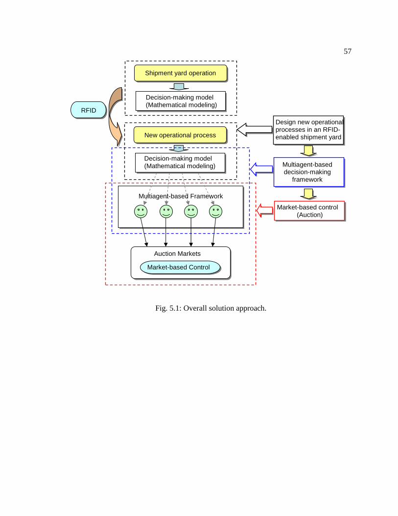
57

Fig. 5.1: Overall solution approach.

Shipment yard operation

Decision-making model (Mathematical modeling)

New operational process

RFID

Auction Markets

Decision-making model (Mathematical modeling)

Multiagent-based Framework

Market-based Control

Design new operational processes in an RFID-enabled shipment yard

Multiagent-based decision-making

framework

Market-based control (Auction)

58

Chapter 6

Vehicle Deployment – Solution Methodology

RFID-enabled real-time location tracking makes the vehicle deployment process

more reliable and visible. In the suggested, RFID-enabled, shipment yard, a vehicle

deployment planner can have real-time awareness of vehicle information in the shipment

yard and the state of parking slots. In order to incorporate real-time information and

handle the dynamics in a vehicle deployment environment, a new operational process for

vehicle deployment and a corresponding mathematical programming model are designed

in this section. As a solution approach for vehicle deployment, this study presents a

multiagent-based decision-making framework which facilitates of a market-based control

mechanism.

6.1 Vehicle Deployment in RFID-enabled Shipment Yard

In the RFID-enabled shipment yard shown in Figure 6.1, a vehicle has an active

RF tag attached before release to the shipment yard. The attached RF tag transmits real-

time information about the vehicle and its location to RFID readers. RFID data server

receives all data collected by the RFID readers. Yard operators obtain work orders via

wireless devices, such as Personal Digital Assistants (PDAs) or tablet PCs. The work

order includes information about the vehicle to be retrieved from the temporary buffer

and its assigned parking slot in the general buffer.

59

Active RF TagRFID Reader

IEEE 802.11x

RFIDData Server

WirelessCommunication

Gateway

Yard Operator withWireless Device

(PDA or Tablet PC)

Vehicle DeploymentPlanner

RFID Tracking System

Active RF TagRFID Reader

IEEE 802.11x

RFIDData Server

WirelessCommunication

Gateway

Yard Operator withWireless Device

(PDA or Tablet PC)

Vehicle DeploymentPlanner


Fig. 6.1: Information architecture for RFID-enabled shipment yard.

The vehicle deployment planner can track currently available parking slots and

vehicles waiting for allocation in real-time. To utilize this information obtained from the

RFID data server, a new vehicle-parking slot allocation strategy needs to consider: (1) the

method for utilizing the real-time information about the vehicles and the available

parking slots to assign initial parking slots to the vehicles released from the plant; (2) the

method for updating the initial vehicle deployment decision to reflect dynamic changes,

as the set of available parking slots changes.

6.1.1 Initial Decision for Vehicle Deployment

Whenever a newly produced vehicle is released to the temporary buffer, the yard

manager obtains the vehicle’s information, such as its delivery destination and loading

location, from a vehicle production information system linked to the vehicle deployment

planner through an interface. The RFID tracking system automatically updates the

currently available parking slots in real-time, and a parking slot allocation decision for

newly produced vehicle i can be made by solving:

60

subject to

where a binary decision variable, ibx , is 1 if parking slot b, ib ∈B , is allocated to vehicle

i, otherwise 0. In the above formulation, the set of available parking slots for vehicle i,

iB , is obtained from the RFID system that detects two sets of parking slots, iEB and i

CB .

iEB is the set of all empty parking slots upon release of vehicle i and i

CB is the set of

empty parking slots allocated to other vehicles currently in the shipment yard but not

completely moved into the assigned parking slots. Figure 6.2 compares the set of

available parking slots for the initial decision model in the RFID-enabled shipment yard

with that for the current best decision model explained in Section 2.4.

, , , ,

i


b B d r w d


s s s s∈

+ + + + + ⋅

∑ (6.1)

1i

ib

b

x∈

=∑B

(6.2)

\i i iE C=B B B (6.3)

{ }0, 1 ,i ibx b∈ ∀ ∈B

61

Fig. 6.2: The set of available parking slots for a vehicle deployment decision in (a) the current best vehicle deployment model, and (b) the initial vehicle deployment decision model.

6.1.2 Updating Vehicle Deployment Decisions

A vehicle released into the temporary buffer requires a certain amount of time

until its movement to a parking slot in the general buffer is complete. Two types of

operational delays explain this amount of time. One is that a vehicle has to stay in the

temporary buffer until a yard operator becomes available to move it, and the other is the

time required to move the vehicle from the temporary buffer to an assigned parking slot

in the general buffer. As discussed in Section 2.3, the set of available parking slots

continuously changes during this time period due to dynamic events. Thus, the initial

deployment decisions made in the previous section should be updated in response to

those changes that may lead to improvement or deterioration of deployment performance.

Huang et al. (2005) emphasize that updating an initial decision should be performed to

The set of available parking slots

at this time point

B

Deployment decisions for individual vehicle

Deployment decisions for individual vehicle

iB iB iB iB

Updating Bi in real-time

(a)

(b)

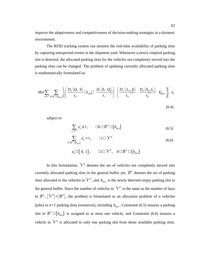
62

improve the adaptiveness and competitiveness of decision-making strategies in a dynamic

environment.

The RFID tracking system can monitor the real-time availability of parking slots

by capturing unexpected events in the shipment yard. Whenever a newly emptied parking

slot is detected, the allocated parking slots for the vehicles not completely moved into the

parking slots can be changed. The problem of updating currently allocated parking slots

is mathematically formulated as:

subject to

In this formulation, PV denotes the set of vehicles not completely moved into

currently allocated parking slots in the general buffer yet, PB denotes the set of parking

slots allocated to the vehicles inPV , and newb is the newly detected empty parking slot in

the general buffer. Since the number of vehicles in PV is the same as the number of bays

in PB , P P=V B , the problem is formulated as an allocation problem of n vehicles

(jobs) to n+1 parking slots (resources), including newb . Constraint (6.5) ensures a parking

slot in { }Pnewb∪B is assigned to at most one vehicle, and Constraint (6.6) ensures a

vehicle in PV is allocated to only one parking slot from those available parking slots.

{ }

, , , ,

P Pnew


i V b B b d r w d


s s s s∈ ∈ ∪

+ + + + + ⋅

∑ ∑

(6.4)

{ }1,P

i Pb new

i

x b b∈

≤ ∀ ∈ ∪∑V

B (6.5)

{ }

1,P

new

i Pb

b b

x i∈ ∪

= ∀ ∈∑B

V (6.6)

{ } { }0, 1 , ,i P Pb newx i b b∈ ∀ ∈ ∈ ∪V B

63

Finally a binary decision variable ibx is 1 if parking slot b is allocated to vehicle i,

otherwise 0.

6.2 Multiagent-based Decision-making Framework

The problem of updating vehicle deployment decisions, discussed in Section

6.1.2, is formulated on the basis of centralized information processing and decision-

making in which the vehicle deployment planner should be aware of all deployment

related information, such as vehicles’ current locations and loading locations, availability

of parking slots, and other dynamic events. Moreover, the above decision problem should

be solved repeatedly upon detection of a new empty parking slot. When the number of

vehicles in the yard increases a great deal and dynamic uncertainties grow, the centralized

decision-making approach may not be adequate for processing a large amount of

distributed information and may be unable to provide prompt decisions.

To overcome the limitations of the centralized decision-making approach, this

study proposes a multiagent-based decision-making framework in which a market-based

control mechanism is facilitated to accommodate the dynamics associated with different

participants and to process large amounts of distributed information.

6.2.1 Design of Agents

The essential issue of designing a multiagent-based decision-making framework

is to define the individual agent. In this case, the updating process of vehicle deployment

decisions requires defining two main agent classes: vehicle agent and yard manager

agent. The fundamental roles of these agents and key information they maintain are as

follows:

� Vehicle Agent: A vehicle agent represents an individual vehicle in the shipment

yard and is responsible for obtaining an available resource, such as a parking slot

in the general buffer. Each vehicle agent maintains vehicle deployment related

64

information, such as current location, loading location, and currently allocated

parking slot.

� Yard Manger Agent: The yard manager agent is responsible for managing and

coordinating a set of parking slots in the general buffer, and interacts with vehicle

agents to update deployment decisions by allocating appropriate parking slots.

The yard manager agent can monitor the state of parking slots in the general

buffer by accessing the RFID data server.

6.3 Market-based Control Mechanism

Due to the nature of the updating process of vehicle deployment decisions,

discussed in the beginning of this section, it is very natural to model the updating process

as a negotiation process between competitive participants (vehicles) which need to

acquire some resources (parking slots) to achieve their individual goals. An auction is one

popular form of market-based control mechanism. For the purpose of handling the

process of updating vehicle deployment decisions in the multiagent decision-making

framework, this study designs two different auction mechanisms: an auction heuristic

mechanism and an ascending price iterative auction mechanism.

6.3.1 Auction Heuristic Mechanism

Once a newly emptied parking slot newb is detected, the yard manager agent opens

an auction market by sending a request for bid (RFB) message to the vehicle agents that

represent the vehicles in PV , the set of vehicles not completely moved into currently

allocated parking slots. The RFB message includes information of parking slot newb . In

the auction heuristic mechanism, a vehicle agent would update the currently allocated

parking slot if a new allocation would provide better utility value. Section 6.4 explains

the details of utility value for a vehicle agent.

65

Let ( )iu b be the utility value of parking slot b for vehicle agent i. A vehicle

agent, after receiving the RFB message from the yard manager agent, computes the utility

value of parking slot newb to determine whether or not the vehicle agent should participate

in the auction market. For example, if vehicle agent i can expect better utility by taking

newb than by keeping the currently allocated parking slot ib , i.e., ( ) ( )i new i iu b u b≥ , then

vehicle agent i decides to participate in the auction market to obtain newb by submitting a

bidding price for newb , as defined by:

However, if no vehicle agent can expect the larger or equal utility value by taking

newb , the market automatically closes.

Once vehicle agents finish submitting their bidding prices for newb , the yard

manager agent determines a wining vehicle agent i∗ that the one who submitted the

highest bidding price:

Now the yard manager agent allocates newb to the winning vehicle agent i∗ and

consequently opens another market by sending a new RFB message to the remaining

vehicle agents in { }\P P i∗=V V . The new RFB message includes information of

parking slot i

b ∗ , which is released from vehicle agent i∗ . The same biding price

submission and winner determination processes continue, as shown in Table 6.1, and this

auction process repeats until no vehicle agent can achieve better utility value from a

parking slot broadcasted to vehicle agents by an RFB message, or no vehicle agent in

PV remains.

( ) ( ) ( )i new i new i ip b u b u b= − (6.7)

( )* arg maxP

i newi

i p b∈

=V

(6.8)

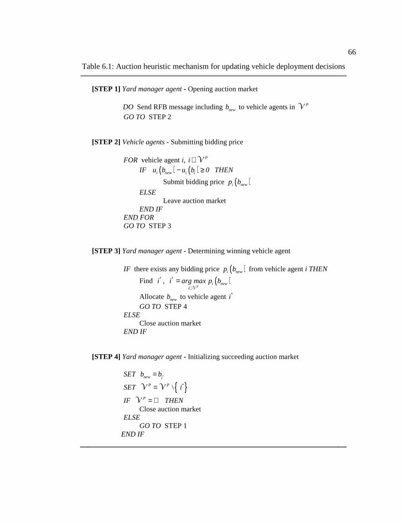
66

Table 6.1: Auction heuristic mechanism for updating vehicle deployment decisions

[STEP 1] Yard manager agent - Opening auction market

DO Send RFB message including newb to vehicle agents in PV

GO TO STEP 2

[STEP 2] Vehicle agents - Submitting bidding price

FOR vehicle agent i, Pi ∈V IF ( ) ( )i new i iu b u b 0− ≥ THEN

Submit bidding price ( )i newp b

ELSE Leave auction market END IF END FOR GO TO STEP 3

[STEP 3] Yard manager agent - Determining winning vehicle agent IF there exists any bidding price ( )i newp b from vehicle agent i THEN

Find i∗ , ( )P

i newi

i arg max p b∗

∈=

V

Allocate newb to vehicle agent i∗ GO TO STEP 4 ELSE Close auction market END IF

[STEP 4] Yard manager agent - Initializing succeeding auction market

SET new ib b ∗=

SET { }\P P i∗=V V

IF P = ∅V THEN Close auction market ELSE

GO TO STEP 1 END IF

67

6.3.2 Ascending Price Iterative Auction Mechanism

The fundamental idea of the proposed ascending price iterative auction

mechanism is from an ε -complementary slackness iterative auction, developed by

Bertsekas (1990) to originally solve n to n allocation problems by matching n jobs to n

resources on a one-to-one basis. Since the problem of updating vehicle deployment

decisions, formulated in Section 6.1.2, is an n vehicles to n+1 parking slots allocation

problem, a dummy vehicle agent is added to an auction market to re-design the problem

as a one-to-one matching allocation problem.

Once a newly emptied parking slot newb is detected, the yard manager agent calls

all the vehicle agents in PV in order to request information of parking slots currently

allocated to vehicle agents. Now, vehicle agent i, Pi ∈V , responds to the yard manager

agent by sending information of its currently allocated parking slot ib . After collecting

information of the set of currently allocated parking slots PB , the yard manager agent

opens an auction market by sending and RFB message to vehicle agents in PV . The

RFB message includes information of the set of all available parking slots including newb ,

{ }Pnewb∪B .

In this auction mechanism, it is supposed that parking slot b has a price ( )p b and

the vehicle agent who takes this parking slot must pay that. Net profit value of parking

slot b for vehicle agent i is the difference between the utility value and the price, that is,

( ) ( )iu b p b− . Through the ascending price iterative auction, parking slots are allocated to

vehicle agents to maximize the total summation of utility values.

The ascending price iterative auction proceeds in iterations starting with current

allocations, where newb is initially allocated to dummy vehicle agent dv and initial prices

of parking slots are set to zero as shown in Figure 6.3.

68

Set of vehicle agents Set of parking slots

vehicle agent 1(b1 is currently allocated)

b1

(initial price p(b1) = 0)

{ }Pdv∪V { }P

newb∪B



vehicle agent n(bn is currently allocated)

dummy vehicle agent ( vd )(bnew is currently allocated)

b2


b3


bn

(initial price p(bn) = 0)

bnew

(initial price p(bnew) = 0)

Yard manageragent

Auction marketSet of vehicle agents Set of parking slots


b1


{ }Pdv∪V { }P

newb∪B



vehicle agent n(bn is currently allocated)

dummy vehicle agent ( vd )(bnew is currently allocated)

b2


b3


bn

(initial price p(bn) = 0)

bnew

(initial price p(bnew) = 0)

Yard manageragent

Auction market

Fig. 6.3: Illustration of design for ascending price iterative auction mechanism which includes a dummy vehicle agent.

Each iteration starts with the allocation result and the set of prices taken from the

previous iteration, and the iteration continues until all vehicle agents are satisfied with the

results of allocation.

As shown in Equation (6.9), vehicle agent i would be satisfied if the net profit

value of allocated parking slot ib is within ε (the minimum price increment) of the

maximum net profit value. However, the assumption is that the dummy vehicle agent is

always satisfied with any result of allocation through all iterations.

At the beginning of each iteration, if is any vehicle agent i is not satisfied with the

previous result of parking slot allocation, this vehicle agent finds parking slot ib∗ that

provides the maximum net profit value:

( ) ( ){ }

( ) ( ){ }maxP

newi i i i

b bu b p b u b p b ε

∈ ∪− ≥ − −

B (6.9)

{ }( ) ( ){ }* arg max

Pnew

i ib b

b u b p b∈ ∪

= −B

(6.10)

69

Once vehicle agent i finds the parking slot ib∗ , the agent exchanges parking slots

with the vehicle agent currently allocated to ib∗ by submitting a new price for parking slot

ib∗ . If ( )new ip b∗ is the new price for parking slot ib∗ , then in this auction market, ( )new ip b∗

is set to a level where vehicle agent i is indifferent between ib∗ and the second best

parking slot, as computed by:

where iα denotes the net profit value of the best parking slot for vehicle agent i and iβ

represents the net profit value of the second best parking slot. The iα and iβ , are

computed as:

By the above definition, the price increment (bidding increment) is always at least

equal to ε .

As described in Table 6.2, the above process in the ascending price iterative

auction mechanism repeats in a sequence of iterations until all vehicle agents are satisfied

with the results of parking slot allocation. The strength of the ascending price iterative

auction market is in computational efficiency and the optimal property of an ε -

complementary slackness auction algorithm (Bertsekas, 1990). When the auction market

terminates, an allocation result is in almost equilibrium and the total sum of utility values

of the final parking slot allocation is within ( )n 1 ε+ ⋅ of being optimal, where n is the

number of vehicle agents in PV .

( ) ( ) ( )* *new i i i ip b p b α β ε= + − + (6.11)

{ }

( ) ( ){ }maxP

newi i

b bu b p bα

∈ ∪= −

B (6.12)

{ } { }( ) ( ){ }

*\max

Pnew i

i ib b b

u b p bβ ∈ ∪

= −B

(6.13)

70

Table 6.2: Ascending price iterative auction mechanism for updating vehicle deployment decisions.

[STEP 1] Yard manager agent - Opening auction market

DO Request currently allocated parking slot ib to vehicle agent i, for Pi∀ ∈V

DO Send RFB message including P newb∪B to vehicle agents in PV GO TO STEP 2

[STEP 2] Vehicle agents - Submitting bidding price

FOR Vehicle agent i, Pi∀ ∈V

IF ( ) ( ){ }

( ) ( ){ }P

newi i i i

b bu b p b max u b p b ε

∈ ∪− ≥ − −

B

THEN

Submit new bidding price ( )new ip b∗ for ib∗

Exchange parking slots with vehicle agent assigned to ib∗

SET ( ) ( )i new ip b p b∗=

ELSE DO Nothing END IF END FOR GO TO STEP 3

[STEP 3] Yard manager agent - Terminating auction market

IF ( ) ( ){ }

( ) ( ){ }P

newi i i i

b bu b p b max u b p b ε

∈ ∪− ≥ − −

B, for Pi∀ ∈V THEN

Close auction market ELSE GO TO STEP 2

END IF

6.4 Design of Utility Function for Vehicle Agent

Design of the utility function of a vehicle agent for a parking slot considers two

principal factors in the vehicle deployment operational environment: consolidated

operational time and shipment loading schedule. Since a vehicle agent has a preference

71

for the parking slot requiring less consolidated operational time, as defined in Equation

(2.5), it makes clear to define the utility value of parking slot b for vehicle agent i,

( )iu b , as a reciprocal form of the consolidated operational time for vehicle i to parking

slot b.

In the shipment yard, vehicles in the general buffer move to designated loading

locations based on a predefined shipment loading schedule. In general, the shipment

loading schedule primarily considers a vehicle’s delivery priority. For example, a vehicle

with a high delivery priority is expected to be shipped earlier than a vehicle with a lower

delivery priority. Table 6.3 describes a simple instance of creating a shipment loading

schedule that follows a high-priority-first-loaded (HPFL) rule. As a result of the HPFL-

based loading schedule, the amount of time a vehicle with a higher delivery priority stays

in a general buffer before moving to a designated loading location is likely to be shorter

than the amount of time a vehicle with a lower delivery priority stays.

( ) ( ){ },1

i iu b COT L b−

= (6.14)

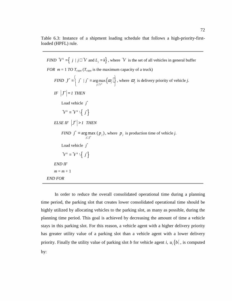
72

Table 6.3: Instance of a shipment loading schedule that follows a high-priority-first-loaded (HPFL) rule.

FIND { }| and kjj j L k= ∈ =V V , where V is the set of all vehicles in general buffer

FOR m = 1 TO Tcapa (Tcapa is the maximum capacity of a truck)

FIND ( )* * *| arg maxk

jj

j j ω∈

= = V

J , where jω is delivery priority of vehicle j.

IF * 1=J THEN

Load vehicle *j

{ }*\k k j=V V

ELSE IF * 1>J THEN

FIND * arg max ( )jj

j p∗∈

=J

, where jp is production time of vehicle j.

Load vehicle *j

{ }*\k k j=V V

END IF

m = m + 1

END FOR

In order to reduce the overall consolidated operational time during a planning

time period, the parking slot that creates lower consolidated operational time should be

highly utilized by allocating vehicles to the parking slot, as many as possible, during the

planning time period. This goal is achieved by decreasing the amount of time a vehicle

stays in this parking slot. For this reason, a vehicle agent with a higher delivery priority

has greater utility value of a parking slot than a vehicle agent with a lower delivery

priority. Finally the utility value of parking slot b for vehicle agent i, ( )iu b , is computed

by:

73

where iω denotes delivery priority of vehicle i. The value of iω is set within 0 to 1,

i0 1ω< < , and larger iω implies higher delivery priority.

( ) ( ) ( ){ }

( )

,

, , , ,

1

i i i

1

d r w i d ii wait load

d r w d

u b 1 COT L b

D Q b D b Q D L b D b L1 t t

s s s s

ω

ω

−

−

= + ⋅

= + ⋅ + + + + +

(6.15)

74

Chapter 7

Empirical Analysis of Vehicle Deployment

Computational experiments conducted with simulation validated the new design

of the market-based control for the vehicle deployment process in the RFID-enabled

shipment yard. This chapter presents the experimental setup followed by the experimental

analysis results.

7.1 Experimental Setup

Computational experiments compare four different vehicle deployment models,

classified in Table 7.1, are compared in terms of consolidated operational time, shipment

yard utilization, and labor consumption. Vehicle deployment models considered in the

experimentation are:

� CVD: Current best vehicle deployment practice model, described in Section 2.4.

� RVDID: RFID-enabled vehicle deployment model with initial deployment

decision only, described in Section 6.1.1.

� RVDID+AH: RFID-enabled vehicle deployment model with updating initial

deployment decisions using the auction heuristic, described in Section 6.3.1.

� RVDID+IA : RFID-enabled vehicle deployment model with updating initial

deployment decision using the ascending price iterative auction, described in

Section 6.3.2.

75

Table 7.1: Classification of vehicle deployment models.

Description Vehicle deployment model

CVD RVDID RVDID+AH RVDID+IA

RFID tracking system No Yes Yes Yes

Initial decision for vehicle deployment

Yes Yes Yes Yes

Updating vehicle deployment decision

No No Yes Yes

Market-based control - - Auction heuristic

Ascending price iterative auction

7.1.1 Experimental Conditions

An illustration of the structure and the size of the shipment yard considered

through the experiments appears in Figure 7.1. The size of the general buffer in the

shipment yard is a grid of 50×100 slots, where the total number of parking slots is 5,000,

and the number of loading locations in the loading buffer is 50. An assembly plant

releases a finished vehicle to the temporary buffer, every 2 time units on average

(uniform distribution on the interval [1.8, 2.2]), and a truck arrives at the loading buffer

every 16 time units, on average (uniform distribution on the interval [14.4, 17.6]). The

number of vehicles a truck can load is set to 8. The vehicle loading sequence follows the

HPFL (high-priority-first-loaded) rule, explained in Section 6.4., and the delivery priority

for each vehicle is randomly selected from a uniform distribution on the interval [0, 1]. It

is assumed that the unit speeds of driving and riding are 10 and 8 times higher than that

of walking. Waiting time for a yard operator, twait, and vehicle loading time for a trucker,

tload, are randomly generated from uniform distributions on the interval [7.0, 9.0] and

[8.0, 12.0], respectively. For each vehicle deployment model, simulation continues for a

total of 20,000 vehicles loaded onto trucks, and a total of 20 simulation runs for each

vehicle deployment model are repeated to reduce random effects.

76

General Buffer (50X100 grid)

50 p

arki

ng s

lot r

ows

100 parking slot columns

50 lo

adin

g ar

eas

Loading Buffer Temporary Buffer

(0, 0) (15, 0)

(135, 100)(0, 100)

(300, 100)

(x, y) : Unit distancecoordinates

General Buffer (50X100 grid)

50 p

arki

ng s

lot r

ows


50 lo

adin

g ar

eas

Loading Buffer Temporary Buffer

(0, 0) (15, 0)

(135, 100)(0, 100)

(300, 100)

(x, y) : Unit distancecoordinates

Fig. 7.1: Structure and size of the shipment yard use for the experiments.

7.2 Consolidated Operational Time

It is obvious that the consolidated operational time depends on the vehicle’s

allocated parking slot in the general buffer. Table 7.2 shows the experimental results for

the average operational times for each elementary operation5 and the average

consolidated operational times for the different vehicle deployment models. The average

operational times for the operations EO-I and EO-II, conducted by a yard operator, are

slightly increased in RVDID, RVDID+AH, and RVDID+IA , as compared to the operational

times in CVD. However the average operational time for EO-III, the walking operation

from a loading location to a parking slot by a trucker, is considerably decreased to

45.03%, 55.67%, and 57.40%, in RVDID, RVDID+AH, and RVDID+IA , respectively. As a

result, the average consolidated operational time for a single vehicle is reduced to 20.15%

in RVDID, 25.75% in RVDID+AH, and 26.84% in RVDID+IA when compared to CVD.

These results indicate that real-time information on vehicles and the availability of

parking slots, provided by the RFID tracking system, creates a significant decrease in a

5 The elementary operations for a yard operator (EO-I and EO-II) and a trucker (EO-III and EO-

IV) are described in Section 2.1.

77

trucker’s operational time, which is a dominant factor of the consolidated operational

time. This fact is quite reasonable because walking from a loading location to a parking

slot is the most time-consuming operation in vehicle deployment.

Table 7.2: Average operational time (unit time) for deployment of a single vehicle.

Operation name Vehicle deployment model

CVD RVDID RVDID+AH RVDID+IA a

Operations for yard operator 56.31 66.59 67.99 68.06

EO-I 21.45 26.04 26.69 26.73

EO-II 26.86 32.55 33.30 33.33

Operations for trucker 108.17 64.74 54.14 52.28

EO-III 88.81 48.82 39.37 37.83

EO-IV 9.36 5.92 4.77 4.45

COT 164.48 131.33 122.13 120.34

a For the ascending price iterative auction algorithm, the value of ε is set to 10-5.

It is also shown that a vehicle deployment decision made by RVDID improves

with updating the vehicle deployment decision using the proposed auction mechanism. In

terms of the average operational time for EO-III, 19.36% and 22.51% are the

improvements for RVDID+AH and RVDID+IA , respectively, as compared to RVDID, and the

average consolidated operational time is enhanced to 7.01% and 8.37% for RVDID+AH

and RDVID+IA , respectively.

7.3 Shipment Yard Utilization

As explained in Chapter 2, the operational time for a trucker depends mainly on

the distance from a vehicle in the general buffer to its loading location. From this fact, it

is clearly noticeable that increasing the utilization of the parking slots near loading

78

locations is important and may result in a reduction of the operational time for a trucker

and, consequently, the consolidated operational time. Investigation of the utilization of a

parking slot in different vehicle deployment models introduces two different performance

measures: a utilization rate of parking slot and a frequency of parking slot utilization.

7.3.1 Utilization Rate of Parking Slot

The utilization rate of a parking slot is defined as the ratio of the time that the

parking slot is occupied by the vehicles during the total simulation time period. Let

( )UR b be the utilization rate of parking slot b. From the result of the simulation study,

( )UR b is computed by:

where V is the set of total vehicles moved into the general buffer during the simulation

time period, and ( )bt v denotes the time period vehicle v has occupied parking slot b.

The following Figures 7.2, 7.3, 7.4, and 7.5 show the utilization rates of parking

slots in CVD, RVDID, RVDID+AH, and RVDID+IA , respectively.

( ) ( )bvt v

UR bTotal simulation time period

∈= ∑ V (7.1)

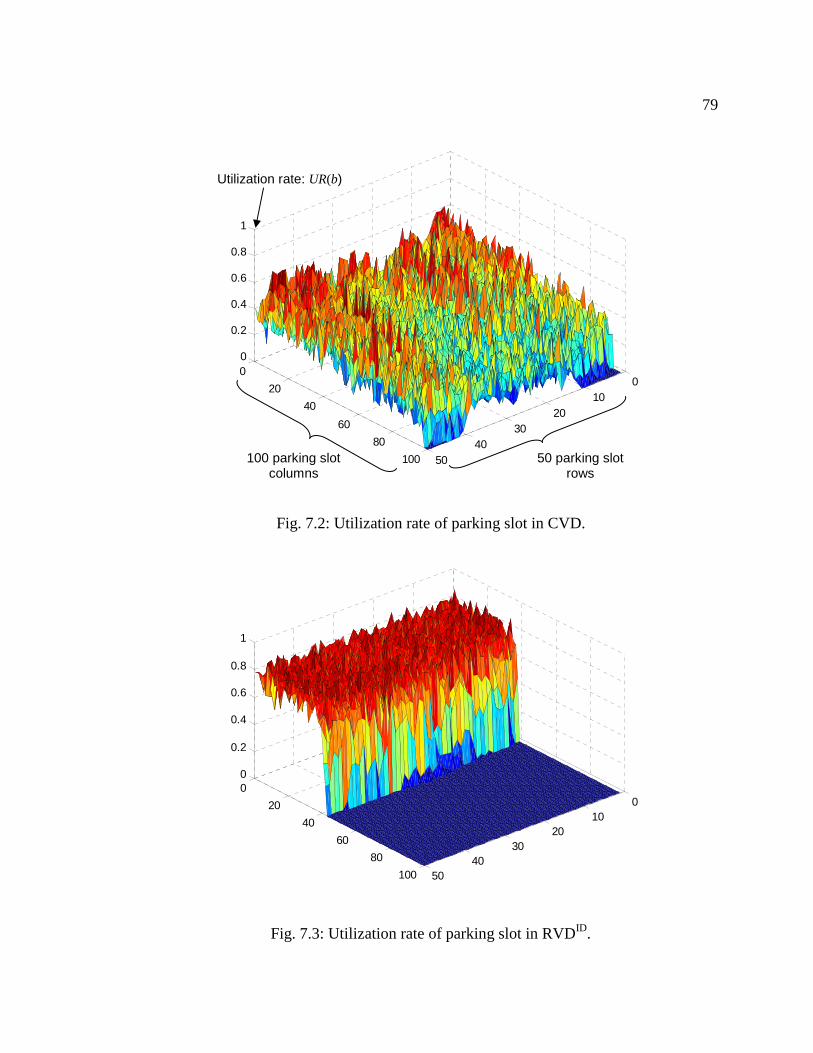
79

Fig. 7.2: Utilization rate of parking slot in CVD.

Fig. 7.3: Utilization rate of parking slot in RVDID.

010

2030

4050

0

20

40

60

80

100

0

0.2

0.4

0.6

0.8

1


50 parking slot rows

Utilization rate: UR(b)

010

2030

4050

0

20

40

60

80

100

0

0.2

0.4

0.6

0.8

1

80

Fig. 7.4: Utilization rate of parking slot in RVDID+AH.

Fig. 7.5: Utilization rate of parking slot in RVDID+IA .

010

2030

4050

0

20

40

60

80

100

0

0.2

0.4

0.6

0.8

1

010

2030

4050

0

20

40

60

80

100

0

0.2

0.4

0.6

0.8

1

81

As shown in the above figures, RFID-enabled vehicle deployment models,

RVDID, RVDID+AH, and RVDID+IA , significantly increase the utilization rate of parking

slots near loading locations as compared to CVD. It is obviously shown in Figure 7.6 that

vehicle deployments by RVDID+AH and RVDID+IA considerably enhance the utilization

rate of parking slots near loading locations.

Fig. 7.6: Average utilization rate of the parking slots (50 parking slots) in each parking slot column.

7.3.2 Frequency of Parking Slot Utilization

The utilization rate of a parking slot itself does not accurately reflect the

utilization of a parking slot. For example, if a certain vehicle occupies the parking slot

preferred for other vehicles for a long time period, this increases the utilization rate of the

parking slot defined in Equation (7.1). However, from the perspective of vehicle

Parking slot column no. (50 parking slots in each column)

closer to loading area further from loading area

0

0.1

0.2

0.3

0.4

0.5

0.6

0.7

0.8

0.9

1

1 5 9 13 17 21 25 29 33 37 41 45 49 53 57 61 65 69 73 77 81 85 89 93 97

CVD

RVD-ID

RVD-ID+AH

RVD-ID+IA

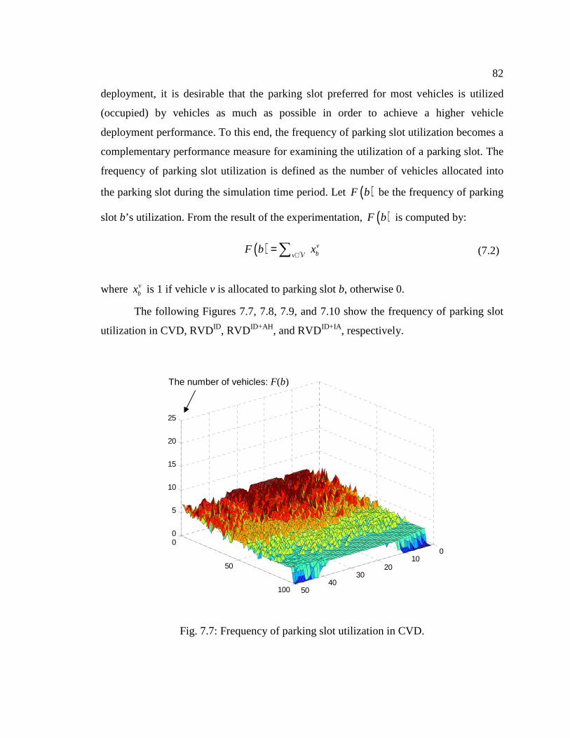
82

deployment, it is desirable that the parking slot preferred for most vehicles is utilized

(occupied) by vehicles as much as possible in order to achieve a higher vehicle

deployment performance. To this end, the frequency of parking slot utilization becomes a

complementary performance measure for examining the utilization of a parking slot. The

frequency of parking slot utilization is defined as the number of vehicles allocated into

the parking slot during the simulation time period. Let ( )F b be the frequency of parking

slot b’s utilization. From the result of the experimentation, ( )F b is computed by:

where vbx is 1 if vehicle v is allocated to parking slot b, otherwise 0.

The following Figures 7.7, 7.8, 7.9, and 7.10 show the frequency of parking slot

utilization in CVD, RVDID, RVDID+AH, and RVDID+IA , respectively.

Fig. 7.7: Frequency of parking slot utilization in CVD.

( ) vbv

F b x∈

=∑ V (7.2)

010

2030

4050

0

50

100

0

5

10

15

20

25

The number of vehicles: F(b)

83

Fig. 7.8: Frequency of parking slot utilization in RVDID.

Fig. 7.9: Frequency of parking slot utilization in RVDID+AH.

010

2030

4050

0

50

100

0

5

10

15

20

25

010

2030

4050

0

50

100

0

5

10

15

20

25

84

Fig. 7.10: Frequency of parking slot utilization in RVDID+IA .

As shown in the previous figures, RFID-enabled vehicle deployment models,

RVDID, RVDID+AH, and RVDID+IA , significantly increase the number of vehicles allocated

to the parking slots near loading locations. In other words, the parking slots providing

high vehicle deployment performance are utilized by a significantly larger number of

vehicles compared to CVD. To clarify this result, Figure 7.11 shows the average number

of vehicles deployed into the parking slots in each parking slot columns (50 parking slots

in each parking slot column). The average number of vehicles parked near loading

locations is considerably more in RVDID+AH and RVDID+IA . This suggests that parking

slots near loading locations are highly utilized by moving vehicles into these slots as

much as possible, resulting in reduction of consolidated operational time. This result also

indicates that the RFID-enabled vehicle deployment models provide a yard manger with

an opportunity to reduce the size of the general buffer while enhancing the performance

of vehicle deployment.

010

2030

4050

0

50

100

0

5

10

15

20

25

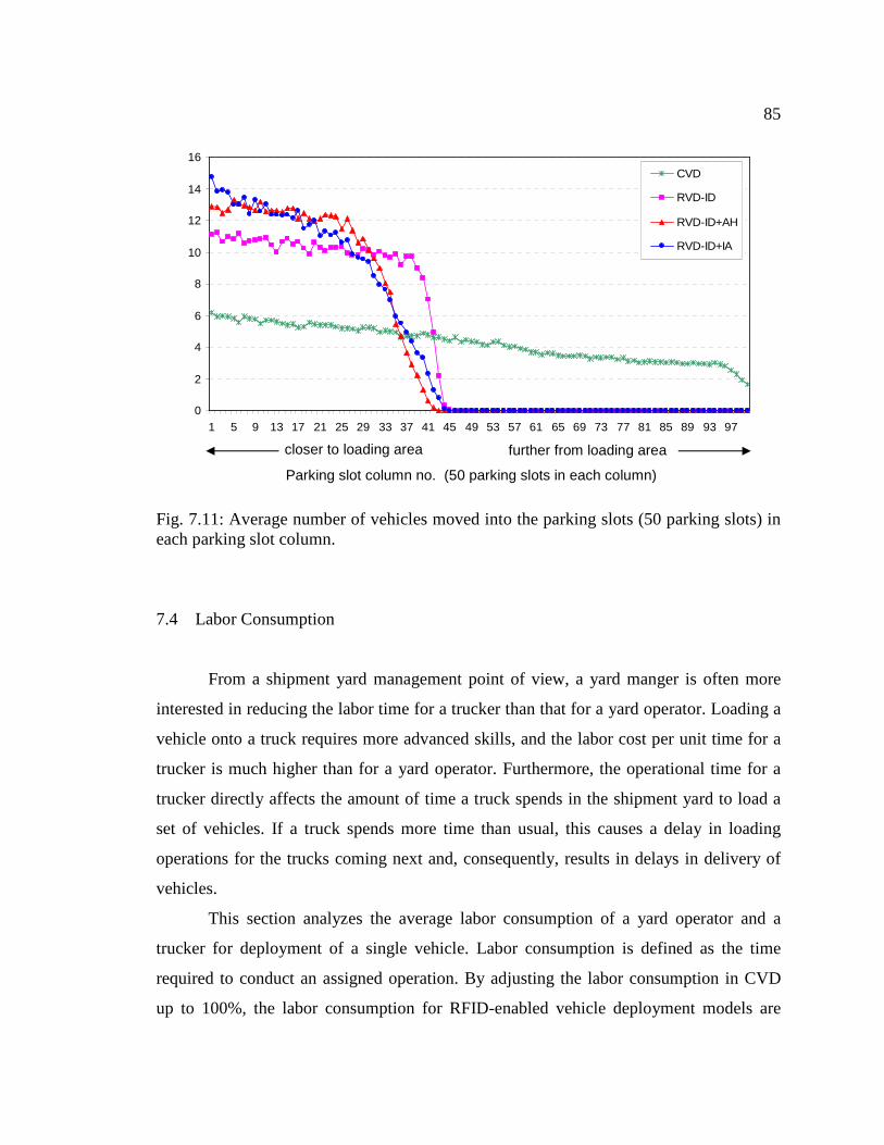
85

Fig. 7.11: Average number of vehicles moved into the parking slots (50 parking slots) in each parking slot column.

7.4 Labor Consumption

From a shipment yard management point of view, a yard manger is often more

interested in reducing the labor time for a trucker than that for a yard operator. Loading a

vehicle onto a truck requires more advanced skills, and the labor cost per unit time for a

trucker is much higher than for a yard operator. Furthermore, the operational time for a

trucker directly affects the amount of time a truck spends in the shipment yard to load a

set of vehicles. If a truck spends more time than usual, this causes a delay in loading

operations for the trucks coming next and, consequently, results in delays in delivery of

vehicles.

This section analyzes the average labor consumption of a yard operator and a

trucker for deployment of a single vehicle. Labor consumption is defined as the time

required to conduct an assigned operation. By adjusting the labor consumption in CVD

up to 100%, the labor consumption for RFID-enabled vehicle deployment models are

0

2

4

6

8

10

12

14

16

1 5 9 13 17 21 25 29 33 37 41 45 49 53 57 61 65 69 73 77 81 85 89 93 97

CVD

RVD-ID

RVD-ID+AH

RVD-ID+IA

Parking slot column no. (50 parking slots in each column)

closer to loading area further from loading area

86

relatively calculated. For example, the labor consumption of a yard operator in vehicle

deployment model m, ( )YOLC m , is computed by:

where ( )YOSOT m denotes the sum of the operational times required for a yard operator to

conduct deployment of a single vehicle in vehicle deployment model m.

As shown in Figures 7.12 and 7.13, although the labor consumption of a yard

operator slightly increases, the labor consumption of a trucker significantly decreases

with the RFID-enabled vehicle deployment models, which leads a reduction of total labor

costs and avoid delays in vehicle loading operations and deliveries.

Fig. 7.12: Average labor consumption of a yard operator with different vehicle deployment models.

( ) ( )( ) = CVD

YOYO

YO

SOT mLC m 100

SOT× (7.3)

0

20

40

60

80

100

120

140

CVD RVD-ID RVD-ID+AH RVD-ID+IA

LCYO (%)

Vehicle deployment models

87

Fig. 7.13: Average labor consumption of a trucker with different vehicle deployment models.

7.5 Summary of Empirical Analysis

The experimental results demonstrate that the RFID-enabled vehicle deployment

models, RVDID, RVDID+AH, and RVDID+IA , outperform the current vehicle deployment

model, CVD, with respect to the selected performance measures. This proves that

applying the RFID technology to a current shipment yard can significantly improve the

performance of vehicle deployment by: (1) reducing the consolidated operational time,

(2) increasing shipment yard utilization, and (3) decreasing labor consumption. Further,

the proposed market-based approach, using the multiagent computational architecture,

improves system performance because this approach can effectively capture and respond

to the dynamic changes in the shipment yard environment by incorporating the large

amount of real-time distributed vehicle location information.

0

10

20

30

40

50

60

70

80

90

100

CVD RVD-ID RVD-ID+AH RVD-ID+IA

LCT (%)

Vehicle deployment models

88

Chapter 8

Shipment Load Makeup – Solution Methodology Part I

In the RFID-enabled shipment yard, the shipment load makeup process can be

more reliable and visible in response to dynamics and uncertainties in the shipment load

makeup operational environment. Incorporating the real-time information from an RFID

system into the shipment load makeup process involves designing a new operational

process and a corresponding mathematical programming model for shipment load

makeup. As a foundation of the solution approach for the new shipment load makeup

process, this chapter presents a multiagent-based decision-making framework.

8.1 Shipment Load Makeup in RFID-enabled Shipment Yard

As explained in Chapter 3, a manual reporting process periodically updates

information on the vehicles in the shipment yard. Yard operators and truckers manually

inform a yard manager of the available vehicles in the shipment yard and their current

locations. Since these manual reporting and updating processes take a certain amount of

time, the availability of vehicles in the shipment yard is not updated immediately and it is

inevitable to make a shipment load makeup plan for a certain time period in advance.

By introducing RFID technology, a shipment load makeup planner receives real-

time information on currently available vehicles and their locations in the shipment yard.

This can make the shipment load makeup process more reliable and adaptable in response

to dynamics and uncertainties. Since the shipment load makeup planner’s information on

all the vehicles is in real-time, the planner can determine the set of vehicles to be loaded

onto a truck just before or when a truck arrives at the yard. In addition, real-time tracking

of vehicle location in the shipment yard eliminates time consumed searching for a

misplaced vehicle.

89

Availability of information on vehicles and their locations in real-time enables the

shipment load makeup planner to decompose a shipment load makeup planning model,

into a set of shipment load makeup decision models, which facilitates a set of decisions

for a certain planning time period. The goal of a shipment load makeup decision model is

to provide a shipment load makeup plan for a single truck whenever that truck actually

arrives at the shipment yard. The real-time shipment load makeup decision model is

illustratively compared to the planning model in Figure 8.1.

Fig. 8.1: Illustrative comparison between shipment load makeup planning model and real-time shipment load makeup decision model.

As illustrated in Figure 8.1, the changes in the set of available vehicles during the

planning time period can be fully reflected through the new shipment load makeup

process in the RFID-enabled shipment yard. In the new shipment load makeup process,

each shipment load makeup decision is made with real-time information on available

vehicles, and uncertain schedules for vehicle production and truck arrivals, which may

degrade performance of the shipment load makeup planning model, are eliminated from a

decision-making process. Thus the new shipment load makeup process, enabled by real-

time information from the RFID system, is more adaptable and flexible in response to the

inevitable dynamics and uncertainties in shipment load makeup operational environment.

Planning time period

Tbegin (t=0) Tend (t=T)

Build a set of decisions at t=0

Make a decision for a truck

Scheduled truck arrival time

Make a decision for a truck

Actual truck arrival time

Shipment load makeup planning model

Real-time shipment load makeup decision model

90

8.2 Shipment Load Makeup Decision in an RFID-enabled Shipment Yard

In the RFID-enabled shipment yard, the shipment load makeup plan no longer

specifies a certain time period, but specifies a single decision epoch in which a truck

actually arrives at the shipment yard. Based on the new shipment load makeup process,

the shipment load makeup decision for each load makeup scenario presented in Chapter 3

(Section 3.4.2) is formulated as an Integer Programming (IP) model.

The IP formulation for the shipment load makeup decision, easily configured

from the formulation for the shipment load makeup planning, presented in Chapter 3,

occurs by reducing the number of trucks and the number decision epochs.

8.2.1 Shipment Load Makeup Decision in Scenario 1

The two binary decision variables are defined as:


, otherwiseb

1 b

0δ

=

, if the vehicles of dealer in block is chosen for shipment

, otherwisebd

1 d bx

0

=

Similar to the shipment load makeup planning, the objective function shown in

Equation (8.1) is a consolidated form of three different objective functions for the

shipment yard, dealers, and the transportation division.

The objective function for the shipment yard, dealers, and the transportation

division appear in Equations (8.2), (8.3), and (8.4), respectively.

( ) ( ) ( ) ( ),bd S bd D bd T b bdF x F x F x F xδ= + + (8.1)

91

� The objective function of the shipment yard:

In the above equation, the set of available vehicles ordered from dealer d in block

b, bdV , is provided from the RFID data server in real-time, and ∆ ( n ct t∆ = − ) denotes

the length of the discrete time period between the making of a decision, ct , and the arrival

of the next truck, nt .

� The objective function of dealers:

� The objective function of the transportation division:

Finally the shipment load makeup decision is formulated as follows:

( ) ( ) ( ) ( )

( ) ( ){ }

( )[ ]

min ,

,

, if ,

, otherwise

bdb

v

v

HD RPS bd bd

b d v

l LHD hd

l l 1

rpvRP

F x 1 x C v C v

where C v c l

c l L 1 LC v

0

∆ ∆∈ ∈ ∈

+∆

∆= +

∆

= − ⋅ +

=

∈ − ∆ +=

∑ ∑ ∑

∑

B D V

(8.2)

( ) ( ) ( ) ( )

( ) ( ){ }

[ ]

( )[ ]

min ,

, if ,

, otherwise

, if ,

,

bdb

v

v

DL LTD bd bd

b d v

l L

dlv v vDL

l 1

ltv vLT

F x 1 x C v C v

c l l 1 L 1where C v

0

c l L 1 LC v

0

ωω

∆ ∆∈ ∈ ∈

+∆

= +∆

∆

= − ⋅ +

∈ − ∆ + −=

∈ − ∆ +=

∑ ∑ ∑

∑

B D V

otherwise

(8.3)

( ),b b

TR UL bd URT b bd b b bd bd bd

b b d b d

F x C x C x Cδ δ Ψ∈ ∈ ∈ ∈ ∈

= ⋅ + ⋅ + − ⋅ ⋅

∑ ∑ ∑ ∑ ∑B B D B D

V (8.4)

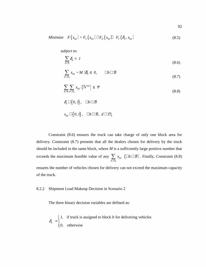
92

subject to:

Constraint (8.6) ensures the truck can take charge of only one block area for

delivery. Constraint (8.7) presents that all the dealers chosen for delivery by the truck

should be included in the same block, where M is a sufficiently large positive number that

exceeds the maximum feasible value of any b

bdd

x∈∑D

( )b∀ ∈B . Finally, Constraint (8.8)

ensures the number of vehicles chosen for delivery can not exceed the maximum capacity

of the truck.

8.2.2 Shipment Load Makeup Decision in Scenario 2

The three binary decision variables are defined as:


, otherwiseb

1 b

0δ

=

( ) ( ) ( ) ( ),bd S bd D bd T b bdMinimize F x = F x F x F xδ+ + (8.5)

bb

1δ∈

=∑B

(8.6)

,b

bd bd

x M 0 bδ∈

− ⋅ ≤ ∀ ∈∑D

B (8.7)

b

bdbd

b d

x Ψ

∈ ∈⋅ ≤∑ ∑

B D

V (8.8)

{ }, ,b 0 1 bδ ∈ ∀ ∈B

{ }, , ,bd bx 0 1 b d∈ ∀ ∈ ∈B D

93

, if truck visits dealer in block for delivering vehicle

, otherwisebd

1 d b

0µ

=

, if vehicle is chosen for shipment (delivery)

, otherwisev

1 vx

0

=

The objective function is a consolidated form of three sub-objective functions for

the shipment yard, dealers, and the transportation division:

The objective function for the shipment yard, dealers, and the transportation

division appear in Equations (8.10), (8.11), and (8.12), respectively.

In the above equations, the set of available vehicles in the shipment yard, V , is

provided from the RFID data server in real-time. Finally the shipment load makeup

decision is formulated as:

( ) ( ) ( ) ( ), ,v S v D v T b bd vF x F x F x F xδ µ= + + (8.9)

( ) ( ) ( ) ( )HD RPS v v

v

F x 1 x C v C v∆ ∆∈

= − ⋅ + ∑V

(8.10)

( ) ( ) ( ) ( )DL LTD v v

v

F x 1 x C v C v∆ ∆∈

= − ⋅ + ∑V

(8.11)

( ), ,b

TR UL URT b bd v b b bd bd v

b b d v

F x C C x Cδ µ δ µ Ψ∈ ∈ ∈ ∈

= ⋅ + ⋅ + − ⋅

∑ ∑ ∑ ∑B B D V

(8.12)

94

subject to:

Constraint (8.15) presents that all the vehicles chosen for delivery by the truck

should be included in the same block, where bV ( )b ⊂V V is the set of vehicles

ordered from dealers in block b, and M1 is a sufficiently large positive number that

exceeds the maximum feasible value of any b

vv

x∈∑V

( )b∀ ∈B . Constraint (8.16) ensures

the truck visits the dealer if it carries any vehicle ordered from the dealer, where bdV

( )bd b⊂ ⊂V V V is the set of vehicles ordered from the dealer d in block b. In this

equation, M2 is an extremely large positive number that exceeds the maximum feasible

value of anybd

vv

x∈∑V

( ), bb d∀ ∈ ∈B D . Finally, Constraint (8.17) ensures the number of

vehicles chosen for delivery can not exceed the maximum capacity of the truck.

( ) ( ) ( ) ( ), ,v S v D v T b bd vMinimize F x = F x F x F xδ µ+ + (8.13)

bb

1δ∈

=∑B

(8.14)

,b

v 1 bv

x M 0 bδ∈

− ⋅ ≤ ∀ ∈∑V

B (8.15)

, ,bd

v 2 bd bv

x M 0 b dµ∈

− ⋅ ≤ ∀ ∈ ∈∑V

B D (8.16)

vv

x Ψ

∈

≤∑V

(8.17)

{ }, ,b 0 1 bδ ∈ ∀ ∈B

{ }, , ,bd b0 1 b dµ ∈ ∀ ∈ ∈B D

{ }, ,vx 0 1 v∈ ∀ ∈V

95

8.3 Shortcomings of Shipment Load Makeup Decision Model in a Distributed Large

Scale Environment

Similar to the shipment load makeup planning, the IP programming of the

shipment load makeup decision has it’s formulation based on centralized information

processing and decision-making. Even though the RFID system provides a decision

maker with real-time information on all the vehicles in the shipment yard, the decision

maker still needs to have shipment load makeup related operational information about

local dealers and the transportation resource division, such as a dealer’s shipment time

commitment for a vehicle, various operational cost functions, etc. Furthermore this

operational information changes frequently as managerial and market environments for

local dealers and the transportation resource division change. With increasing dynamics

and uncertainties in the shipment load makeup environment, the centralized decision-

making approach becomes inadequate in processing all the distributed information and is

unable to provide an adaptable decision in response to the dynamics and uncertainties.

From a computational complexity perspective, even though the shipment load

makeup decision is relatively less complex as compared to the shipment load makeup

planning, the computational complexity of the problem is still significant. In the IP

formulation for the shipment load makeup decision, the number of variables increases

rapidly in relationship to the increase in the number vehicles in the shipment yard, the

number of block areas, and the number of local dealers. Moreover the shipment load

makeup decision is an operational problem addressed on a frequent basis whenever a

truck arrives, and should provide an adaptable solution in time. Thus, it is inevitable to

consider other alternatives rather than a global optimization model, in order to handle the

shipment load makeup decision on a large scale real shipment yard environment.

8.4 Multiagent Architecture for Shipment Load Makeup in an RFID-enabled Shipment

Yard

96

Due to the limitations of a centralized decision-making approach and

computational inefficiency, implementing a global optimization model for shipment load

makeup decisions is inadequate. To overcome these shortcomings when applying the IP

formulation of the shipment load makeup decision to a large scale shipment yard

environment, this study proposes a design for a multiagent-based decision-making

architecture.

The core issue in designing the multiagent architecture for the shipment load

makeup process is defining the individual agent in this architecture. Two major

approaches for defining an agent are possible: (i) function-oriented approach, where

agents represent some functions such as order acquisition, planning, material handling,

and product distribution, or (ii) physical entity-oriented approach, in which agents

represent physical entities such as manager, workers, machines, and components (Shen

and Norrie, 1999). Since the second approach enables an individual agent to manage

efficiently individual local information with limited interactions, the physical entity-

oriented approach is more suitable for modeling a supply chain environment, involving a

large number of physical entities (Lee, 2002). On the basis of this argument, the

following main agent classes are defined: dealer agent (DA), yard agent (YA), block

agent (BA), resource manager agent (RM), resource agent (RA), and market coordinator

agent (MC). The first five agent types embody approximately physical shipment load

makeup organizations, while the MC is a virtual entity for market establishment’s

purpose. The fundamental roles of these agents and the key information entities they

maintain are:

1. Dealer Agent (DA): a DA class agent represents a local dealer and is responsible

for obtaining an available resource, such as a set of vacancies in a truck. The

number of total DAs is equal to the number of local dealers and the set of DAs,

DA , is represented as { }DA | , andbd bb d= ∈ ∈DA B D . Each DA maintains

managerial and operational information of a local dealer, and also has information

on the set of currently available vehicles ordered by a dealer that a DA represents.

For example, DAbd has information on bdV ,

97

{ }| and bdv v bv b d= ∈ ∈V B D .

2. Yard Agent (YA): the YA is responsible for managing information about the

vehicles in the shipment yard by accessing the RFID data server. The YA interacts

with a DA to provide information on the available vehicles ordered by a DA.

Figure 8.2 illustrates the interaction among the YA, the RFID data server, and

DAs.

Fig. 8.2: Interaction among the YA, the RFID data server, and DAs.

3. Block Agent (BA): a BA class agent is designed to represent a block area, and the

set of BAs, BA , is represented as { }BA |b b= ∈BA B . A BA is in charge of

coordinating a set of DAs included in its own block area, and interacts with a

market coordinator agent for temporary economy initiation and clearing. Each BA

maintains information on dealers included in its own block area.

4. Resource Manager Agent (RM): the RM is responsible for representing the

transportation resource division, managing a set of resource agents, and

interacting with the market coordinator agent for temporary economy initiation

YA

DA

Block area 3

DA

DA

DA

Block area 2

DA

DA

DA

Block area 1

DA

DA

Access / Refer Request

Response

RFID data server RFID reader


Active RF tag

98

and clearing. The RM maintains the managerial and operational information of the

transportation resource division.

5. Resource Agent (RA): an RA class agent is responsible for a single transportation

resource, such as a truck, belonging to the transportation resource division. An

RA, as a seller, interacts with BAs or DAs in an auction market. Each RA

maintains information on a truck.

6. Market Coordinator Agent (MC): the MC is responsible for coordinating multiple

auction markets in the temporary economy. The MC is a permanent agent, while

other agents are dismissed from system after achieving their goals.

According to the role definitions of each agent class, the design of an auctioning

process embodies auction mechanisms to handle shipment load makeup decision in the

RFID-enabled shipment yard. This study introduces two different auctioning processes to

handle different shipment load makeup scenarios presented in Chapter 3 and to address

impact of communicational and computational aspects of agents on designing an auction

mechanism. The details of the auctioning processes with corresponding auction

mechanisms follow in Chapters 9 and 10, respectively.

99

Chapter 9

Shipment Load Makeup – Solution Methodology Part II

As explained in Chapter 8, the design of the multiagent-based auctioning process

handles the shipment load makeup decisions in an RFID-enabled shipment yard. For the

shipment load makeup decision in Scenario 1, explained in Section 8.2.1, this chapter

presents the two-tier auctioning process consisting of two different types of auctions, the

first round local auction and the second round central auction. The following sections

present the two-tier auctioning process by detailing market organizations and auction

mechanisms for the first round local auction and the second round central auction.

9.1 The First Round Local Auction

9.1.1 Construction of the First Round Local Auction Market

Once a truck arrives at the shipment yard for the delivery of vehicles, i.e., one of

RAs becomes available, the RM which manages RAs informs the MC of the availability

of an RA (a truck). At this point, the MC initiates a temporary economy for the two-tier

auctioning process. In the temporary economy, each BA establishes the first round local

auction market by sending a request for bid (RFB) message to the corresponding DAs.

Thus, the first round local auction market is established for each block area, and total B

auction markets, where B is the number of block areas, are constructed simultaneously.

Figure 9.1 describes the initiation of a temporary economy and the multiple first round

local auction markets.

100

Fig. 9.1: Construction of the first round local auction markets.

In the first round, each auction market proceeds independently to determine a set

of provisional winning DAs (buyers) which will advance to the second round central

auction market, and DAs only belonging to the same local auction market compete with

each other. Virtually allocating a set of vacancies on the truck to a set of DAs determines

provisional winning DAs for each local auction market.

An iterative bundle auction mechanism, which maximizes the sum value across

the agents in the market, is developed for an auctioning process for each first round local

auction market. The proposed auction mechanism is applied independently to all the local

auction markets in the first round. This section presents the iterative bundle auction

mechanism by detailing the auction process in a certain first round local auction market,

M 1stb ( )b ∈B .

BA

DA

First round local auction market

BA

DA

RM

RA

RA

RA

RA

RA

MC

BA

DA

DA

DA

RFB

RFB



Temporary Economy

RFB

101

9.1.2 Descriptions of Bundle Expression for Identical Items

In the delivery chains of an automobile manufacturer, the transportation resource

division desires that the vehicles, currently available for delivery and ordered from the

same dealer, are shipped together to reduce operational cost by reducing the number of

dealers the truck visits. A dealer also may want all of the available vehicles ordered to be

shipped together in that it is much efficient for the dealer to track orders and to build or

update an inventory plan. Furthermore, in order to design an efficient auction mechanism

for a large scale shipment load makeup environment, considering a set of vehicles

ordered from the same dealer together as one entity will be computationally efficient.

Based on these operational reasons, the design requires that a DA requests a

bundle of vacancies on the truck to allow all the available vehicles the DA has to load on

the truck. In the iterative bundle auction mechanism, DAs are supposed to have non-

additive values for individual vacancies. For example, each DA requires a bundle of

vacancies, which allow of loading all the vehicles it has, while receiving an insufficient

number of vacancies has no value. Vacancies on a truck are regarded as items allocated

(or sold) to DAs through an auction market.

Let G be the set of vacancies on the truck, and bD represents the set of DAs

participating in the first round local auction market for block area b, M 1stb . As a matter of

convenience for representing the index, D and M 1st are used rather than bD and M 1stb in

this chapter6.

Let ( )iu J be the utility value of the bundle of vacancies J ( )J ⊂G for dealer

agent i, DA i ( )i ∈D . Since DAs are supposed to have non-additive value for vacancies

that are regarded as identical items through an auction market, DA i has a certain positive

6 Since each local auction market established in the first round proceeds independently with the same auction mechanism, this chapter presents the auction mechanism in the domain of a certain first round local auction market, and omits the block index b (b∈B) for convenience in mathematical presentation.

102

value iµ for bundle J, only if the number of vacancies in the bundle J, J , is greater than

or equal to the number of vehicles DA i has, iV , otherwise ( )iu J is zero as shown in

Equation (9.1):

From the definition of the utility value of the bundle of vacancies J for DA i , the

implication is that DA i is interested in taking only the bundles where the number of

vacancies is greater than or equal to iV for iµ , and DA i is free to dispose of

unnecessary vacancies. For this reason, the utility value of the bundle where the number

of vacancies is greater than iV might also be set to iµ . Table 9.1 shows the small size

instance of DA valuations for vacancies on a truck.

Table 9.1: DA valuations for vacancies on a truck.

Vacancy (Item)

Agent {A} {B} {C} {A, B} {A, C} {B, C} {A,B,C}

DA1 0 0 0 70 70 70 70

DA2 30 30 30 30 30 30 30

DA3 0 0 0 0 0 0 90

There are three available vacancies (A, B, and C) on a truck and three DAs (DA1,

DA2, and DA3), with the number of vehicles DA1, DA2, and DA3 have are 2, 1, and 3,

respectively. In this table, the utility value for each DA is arbitrarily given.

Since every DA has a non-additive value for an individual vacancy and each

vacancy is an identical item, it is useful to explicitly represent the above table for DA

valuations as Table 9.2, where DA valuations for the bundles can be concisely implicated

as the valuation for the set of bundles which have the same number of vacancies. In this

table bundle J is represented as { } { } { } { } { } { } { }{ }A , B , C , A, B , A, C , B, C , A, B, CJ ∈ .

( ), if and

, otherwise

i i

i

J Ju J

0

µ ≥ ⊂=

V G (9.1)

103

Table 9.2: New representations of DA valuations for identical vacancies (items).

The number of vacancies in bundle J : ( | J | )

Agent | J | =1 | J | =2 | J | =3

DA1 0 70 70

DA2 30 30 30

DA3 0 0 90

From DAs’ valuations for items and the auction mechanism perspectives, the

proposed maximum number of possible bundles considered through the auction

mechanism can be significantly reduced compared to the number considered through the

general bundle auction. In general, bundle auction models are designed to trade non-

identical items between sellers and buyers.

If G is the set of items, and a total G number of items exists, then in general

bundle auction models where each item is regarded as non-identical, the set of possible

bundles, J , and the maximum number of possible bundles, J , are computed by:

{ } { }{ }

| and | and

| and

1 2 G

J J 1 J J J 2 J

J J G J

= ∪ ∪ ∪

= = ⊂ ∪ = ⊂ ∪

∪ = ⊂

J J J J

J J

J

L

L (9.2)

( ) ( ) ( )! ! !

! ! ! ! ! !

1 2 G

G

G G G

1 2 G

G G G

1 G 1 2 G 2 G G G

2 1

= + + +

= + + +

= + + +⋅ − ⋅ − ⋅ −

= −

J J J JL

L

L

(9.3)

104

where kJ ( )k ⊂J J denotes the set of bundles that include k items. As derived in

Equation (9.3), if the number of items increases in a general bundle auction model, the

maximum number of possible bundles increases exponentially. For that reason, general

bundle auction models are not practically applicable for real-world large scale problems

where the number of items required to be allocated is significantly large.

Through the auction mechanism for the shipment load makeup decision, a

vacancy on a truck, allocated (or sold) to DAs, is regarded as an identical item. This fact

enables design of a new bundle expression which makes the auction mechanism

computationally efficient and applicable to large scale real-world problems. The key idea

of the new bundle expression is that the bundles having the same number of items are

regarded as identical bundles through the auction mechanism. Thus, the maximum

number of possible bundles considered in the new bundle expression is computed by:

Figure 9.2 shows the growth of the maximum number of possible bundles in a

general bundle auction model and for the proposed auction model. As the number of

items required to be traded increases, the maximum number of possible bundles

considered in the proposed auction model becomes considerably smaller compared to a

general bundle auction model.

1 2 G G= + + + =J J J JL (9.4)

105

0

50

100

150

200

250

300

1 2 3 4 5 6 7 8

The number of items

Th

e m

axim

al n

um

ber

of

po

ssib

le b

un

dle

s

Proposed Auction Model

General Bundle Auction Model

Fig. 9.2: Growth of the maximum number of possible bundles.

9.1.3 Overall Procedure of Iterative Bundle Auction Mechanism

The iterative bundle auction mechanism proceeds in iterations starting with any

allocation. The asking prices from an auctioneer are initially set to zero for every bundle

in a market. As defined in Chapter 8, a BA plays the role of auctioneer in charge of

controlling the first round local auction market and coordinating the DAs participated in

the market. At the beginning of each iteration, the BA announces to DAs the asking

prices for the bundles. Based on the asking prices, each DA decides whether to place a

bid or not. If a DA decides to place a bid, the DA submits bidding prices for the bundles.

Once the BA receives all of the bids from DAs, the BA determines a temporary allocation

of bundles, and then updates the asking prices for bundles based on the result of the

temporary allocation. At the beginning of the next iteration, the BA informs DAs of the

result of the temporary allocation from the previous iteration and of the new asking

prices. The auction market terminates when all the DAs who placed bids are “satisfied.”

A DA is “satisfied” at the end of an iteration if the DA receives one of the bundles as a

result of a bid. The overall procedure of the iterative bundle auction mechanism appears

in Figure 9.3.

106

Fig. 9.3: Overall procedure of the iterative bundle auction mechanism for the first round local auction market.

9.1.4 Dealer Agent Bidding Strategy

9.1.4.1 Exclusive-Or (XOR) Bid

The iterative bundle auction mechanism allows a DA to place a bid for multiple

bundles. Since a DA wishes to obtain only one bundle from a set of bundles, a DA places

an exclusive-or (XOR) bid for a set of bundles. For instance, Equation (9.5) indicates an

XOR bid placed by DA i for bundles, 1J and 2J , at bidding prices, ( )bid i 1p J and

( )bid i 2p J , respectively:

t = t + 1

Market termination

Yes

No

Initiate auction market

Request for bids

Initial allocation and asking prices

Place bids with bidding prices

Temporary allocation

Close auction market

Updating asking prices

Iterative Bundle Auction Mechanism

107

The above XOR bid implies that DA i desires to obtain, at most, one of bundles

1J and 2J at corresponding bidding prices.

9.1.4.2 Myopic Best-Response Bidding Strategy

In the first round local auction market, a DA follows the myopic best-response

bidding strategy introduced by Parks and Ungar (2000). With this bidding strategy, a DA

submits an XOR bid for the bundles for which (1) every bundle has non-negative profit

value, and (2) every bundle has profit value that is within ε of maximum profit. The

profit value of a bundle is the difference between utility value and price. For example, the

set of bundles in XOR bid from DA i , XORiΠ , is represented as:

where ( )iu J denotes the utility value of bundle J for DA i , and J is the set of all

possible bundles. The second condition, remaining within ε of maximum utility, assures

that the increment of bidding price is always at least equal to ε .

In order to set the bidding price for bundle J as low as possible, a DA submits a

bidding price for bundle J that is equal to the asking price announced by the BA at the

beginning of the iteration. However, if a DA received any bundle thorough a temporary

allocation at a certain iteration t, the DA must repeat the same bid with the same bidding

price at the iteration t+1 even if the asking price for the bundle has increased. By this

agreement, the BA is guaranteed to receive monotonically increasing revenue at each

iteration. For every DA, the rule of setting the bidding price for bundle J is represented

as:

( ) ( ){ }, ,1 bid i 1 2 bid i 2J p J XOR J p J (9.5)

( ) ( ) ( ){( ) ( ) ( ) ( ) }

, | andXORi bid i i bid i

i bid i i bid iJ

J p J u J p J 0

u J p J max u J p J ε∈

Π = − ≥

− ≥ − − J%

% %

(9.6)

108

where ( )task p J denotes the asking price for bundle J announced from the BA at iteration

t.

9.1.4.3 Second-Chance Bidding Strategy

To enhance the performance of the proposed auction mechanism by increasing

DAs’ profits and BA’s revenue, the design for the second-chance bidding strategy

supports the myopic best-response bidding strategy.

At a certain iteration t, if DA i has negative profit values for all of bundles that DA i is

interested in, ( ) ( ) ,ti ask iu J p J 0 J− < ∀ ∈ J where iJ denotes the set of bundles that

DA i is interested in, DA i does not place a bid for any bundle. In this situation, the

second-chance bidding strategy allows DA i to remain in the auction market until the

next iteration t+1, instead of letting DA i leave the market directly. This is called as the

“stay” state of DA i . Now, DA i investigates changes of an asking price for any bundle in

iJ at iteration t+1. Depending on the changes in asking prices, the second-chance

bidding strategy allows DA i to response as follows:

CASE 1: If an asking price of any bundle J ( )iJ ∈ J at iteration t+1 drops from the

asking price at iteration t and DA i has a non-negative profit value for the

bundle J, according to:

( ) ( ) ( ) ( ) , for anyt 1 t t 1ask ask i ask ip J p J u J p J 0 J+ + < ∧ − ≥ ∈ J

( )( )

( )

, if DA received any bundle through the

temporary allocation at the iteration -1 ,

, otherwise

for DA

t 1bid i i

tbid i

task

i

p J

tp J

p J

−=

∀ ∈DA

(9.7)

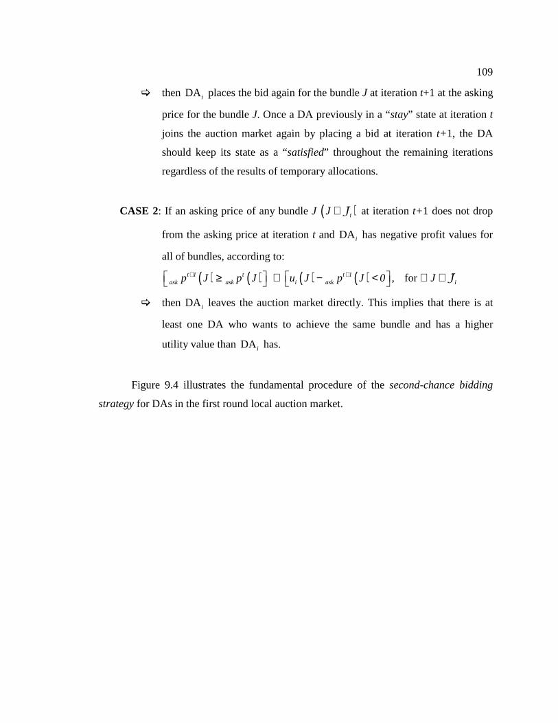
109

� then DA i places the bid again for the bundle J at iteration t+1 at the asking

price for the bundle J. Once a DA previously in a “stay” state at iteration t

joins the auction market again by placing a bid at iteration t+1, the DA

should keep its state as a “satisfied” throughout the remaining iterations

regardless of the results of temporary allocations.

CASE 2: If an asking price of any bundle J ( )iJ ∈ J at iteration t+1 does not drop

from the asking price at iteration t and DA i has negative profit values for

all of bundles, according to:

( ) ( ) ( ) ( ) , for t 1 t t 1ask ask i ask ip J p J u J p J 0 J+ + ≥ ∧ − < ∀ ∈ J

� then DA i leaves the auction market directly. This implies that there is at

least one DA who wants to achieve the same bundle and has a higher

utility value than DA i has.

Figure 9.4 illustrates the fundamental procedure of the second-chance bidding

strategy for DAs in the first round local auction market.

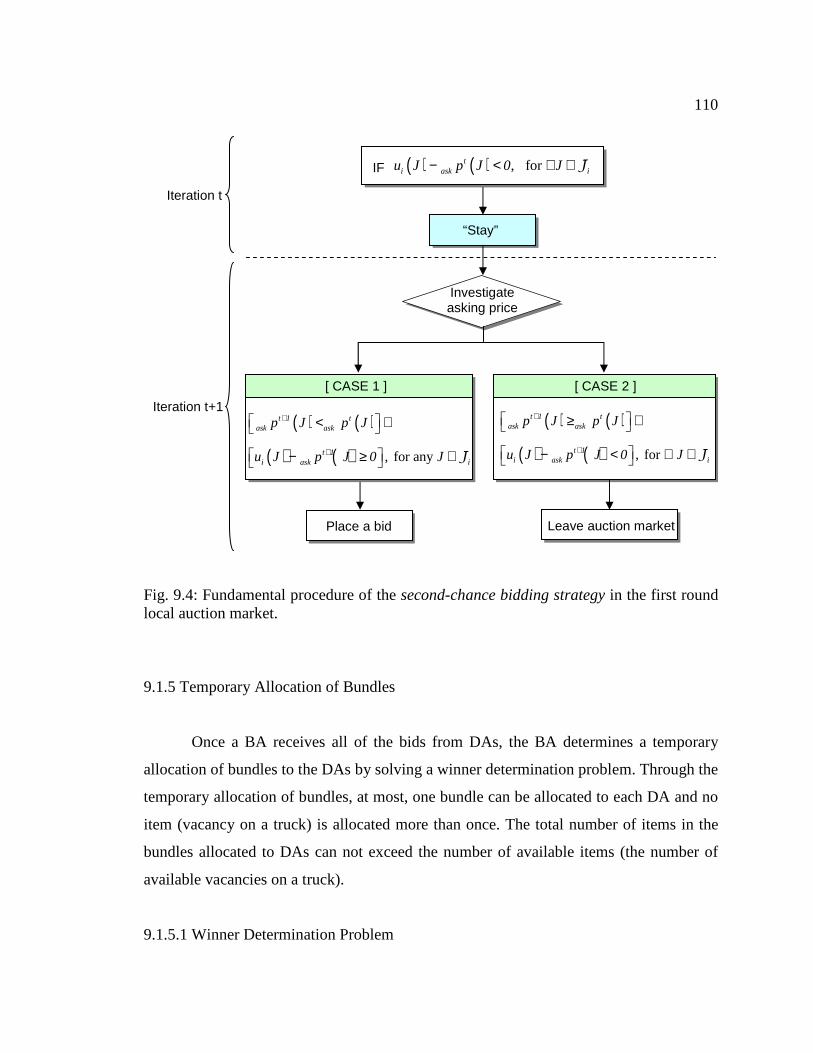
110

Fig. 9.4: Fundamental procedure of the second-chance bidding strategy in the first round local auction market.

9.1.5 Temporary Allocation of Bundles

Once a BA receives all of the bids from DAs, the BA determines a temporary

allocation of bundles to the DAs by solving a winner determination problem. Through the

temporary allocation of bundles, at most, one bundle can be allocated to each DA and no

item (vacancy on a truck) is allocated more than once. The total number of items in the

bundles allocated to DAs can not exceed the number of available items (the number of

available vacancies on a truck).

9.1.5.1 Winner Determination Problem

“Stay”

IF

Iteration t

Iteration t+1

Investigate asking price

Place a bid

( ) ( )

( ) ( ) , for any

t 1 task ask

t 1i ask i

p J p J

u J p J 0 J

+

+

< ∧

− ≥ ∈ J

[ CASE 1 ] [ CASE 2 ]

( ) ( )

( ) ( ) , for

t 1 task ask

t 1i ask i

p J p J

u J p J 0 J

+

+

≥ ∧

− < ∀ ∈ J

Leave auction market

( ) ( ) , forti ask iu J p J 0 J− < ∀ ∈ J

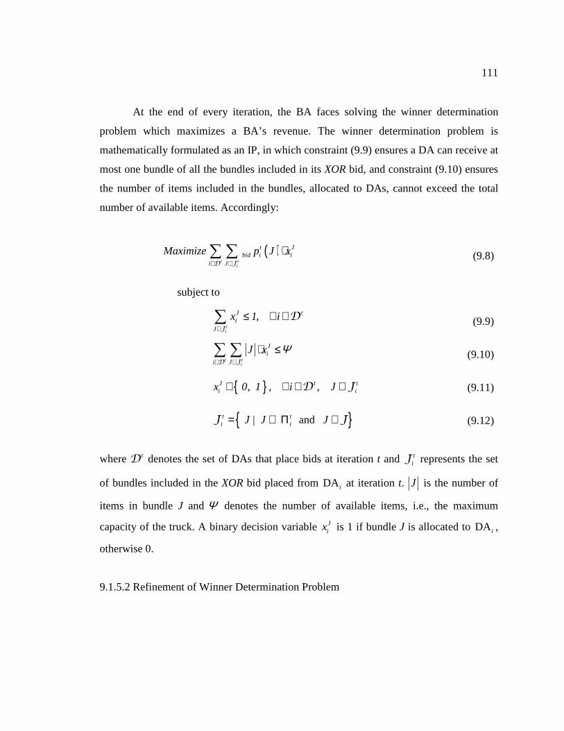
111

At the end of every iteration, the BA faces solving the winner determination

problem which maximizes a BA’s revenue. The winner determination problem is

mathematically formulated as an IP, in which constraint (9.9) ensures a DA can receive at

most one bundle of all the bundles included in its XOR bid, and constraint (9.10) ensures

the number of items included in the bundles, allocated to DAs, cannot exceed the total

number of available items. Accordingly:

subject to

where tD denotes the set of DAs that place bids at iteration t and tiJ represents the set

of bundles included in the XOR bid placed from DA i at iteration t. J is the number of

items in bundle J and Ψ denotes the number of available items, i.e., the maximum

capacity of the truck. A binary decision variable Jix is 1 if bundle J is allocated to DA i ,

otherwise 0.

9.1.5.2 Refinement of Winner Determination Problem

( )t t

i

t Jbid i i

i J

Maximize p J x∈ ∈

⋅∑ ∑D J

(9.8)

,ti

J ti

J

x 1 i∈

≤ ∀ ∈∑J

D (9.9)

t t

i

Ji

i J

J x Ψ∈ ∈

⋅ ≤∑ ∑D J

(9.10)

{ }, , ,J t ti ix 0 1 i J∈ ∀ ∈ ∈D J (9.11)

{ }| and t ti iJ J J= ∈ Π ∈J J (9.12)

112

The original winner determination problem formulated in the previous section can

be refined by studying the characteristics of the auction market in the first round, where

each item is identical with others and a DA has non-additive value for an item.

In the original winner determination problem, the BA investigates all of the

bundles included in a DA’s XOR bid. However the full investigation procedure can be

refined by allowing the BA to examine only the bundle with the smallest number of items

in a DA’s XOR bid. The basic idea for this refinement of the winner determination

procedure is to provide the BA with an opportunity to increase revenue by allocating

surplus items to other DAs.

The refined winner determination procedure also enables a DA to receive a

greater profit by obtaining a bundle at a lower bidding price. The DA’s bidding strategy,

explained in Section 9.1.4, induces the following conditional statement is always true:

This statement guarantees that the bidding price for the bundle including the

smallest number of items among all of bundles in an XOR bid is always smaller than or

equal to those for other bundles in this XOR bid. From this fact, it is clear that the refined

procedure provides a DA with an opportunity to receive a greater profit by obtaining a

bundle at a lower bidding price, while the bundle gives the DA the same utility value

with other bundles in a DA’s XOR bid.

Finally this refined winner determination procedure will promise an allocative

efficiency, which provides the result of allocation that maximizes the sum of the revenue

for the BA (virtual seller) and the profit values for DAs (buyers) in the market. Based on

the refined winner determination procedure, a new winner determination problem is

formulated as:

( ) ( )If , and m n i m n bid i m bid i nJ J J J p J p J∈Π < ⇒ ≤ (9.13)

113

subject to

where *iJ represents the bundle that includes the smallest number of items among all of

bundles in a DA i ’s XOR bid. Constraint (9.15) ensures the total number of items

allocated to DAs can not exceed the total number of available items and a binary decision

variable ix is 1 if bundle *iJ is allocated to DA i , otherwise 0.

9.1.5.3 Effective Winner Determination Algorithm

At the end of every iteration the BA must determine a temporary allocation of

bundles by solving the winner determination problem formulated in Section 9.1.5.2.

Providing an adaptable temporary allocation of bundles to DAs in time is an important

issue in implementing the iterative bundle auction mechanism in real-world applications,

where an auction market is established frequently and the market is supposed to be closed

on time. Introduction of a greedy approach accomplishes the adaptable temporary

allocation of bundles. It provides efficiency for both in solution quality and

implementation. Many studies have shown that a greedy approach offers a satisfactory

performance for large-scale winner determination problems occurring in practical

applications, where multiple items are sold simultaneously and a large number of bidders,

who can express complementarity among these items, participate (Sakurai et al., 2000;

Bassamboo et al., 2001).

( )*t

tbid i i i

i

Maximize p J x∈

⋅∑D

(9.14)

*t

i ii

J x Ψ∈

⋅ ≤∑D

(9.15)

{ }, , tix 0 1 i∈ ∀ ∈D (9.16)

* arg minti

iJ

J J∈

=J

(9.17)

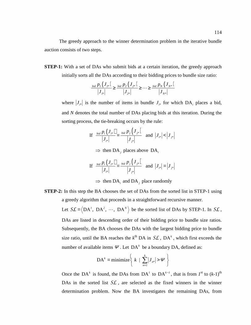
114

The greedy approach to the winner determination problem in the iterative bundle

auction consists of two steps.

STEP-1: With a set of DAs who submit bids at a certain iteration, the greedy approach

initially sorts all the DAs according to their bidding prices to bundle size ratio:

( ) ( ) ( )* * *

* * *

bid 1 1 bid 2 2 bid N N

1 2 N

p J p J p J

J J J≥ ≥ ≥L

where *iJ is the number of items in bundle *iJ for which DA i places a bid,

and N denotes the total number of DAs placing bids at this iteration. During the

sorting process, the tie-breaking occurs by the rule:

( ) ( )*** *

* *

If and

then DA places above DA

bid j jbid i ii j

i j

j i

p Jp JJ J

J J

= <

⇒

( ) ( )*** *

* *

If and

then DA and DA place randomly

bid j jbid i ii j

i j

i j

p Jp JJ J

J J

= =

⇒

STEP-2: In this step the BA chooses the set of DAs from the sorted list in STEP-1 using

a greedy algorithm that proceeds in a straightforward recursive manner.

Let DA , DA , , DA1 2 N=SL L be the sorted list of DAs by STEP-1. In SL ,

DAs are listed in descending order of their bidding price to bundle size ratios.

Subsequently, the BA chooses the DAs with the largest bidding price to bundle

size ratio, until the BA reaches the kth DA in SL , DA k , which first exceeds the

number of available items Ψ . Let DA k be a boundary DA, defined as:

*DA minimize |k

kn

n 1

k J Ψ=

= >

∑

Once the DA k is found, the DAs from DA1 to DA k 1− , that is from 1st to (k-1)th

DAs in the sorted list SL , are selected as the fixed winners in the winner

determination problem. Now the BA investigates the remaining DAs, from

115

(k+1)th to Nth DAs, with their bundle sizes if the remaining items, *

k 1

nn 1

JΨ −−

=∑ ,

can be allocated to any other DAs. To facilitate the listing of the pseudo code for

this procedure, some notations are defined. If S is the set of the selected DAs

and R denotes the available number of items, then the pseudo code of the greedy

algorithm for selecting the DAs (winners) from the sorted list SL is:

SET = ∅S , R Ψ= , n 1= ; WHILE ≠ ∅SL or R 0≠ {

IF *nJ R≤ THEN

{ }DA n= ∪S S ; *nR R J= − ;

ELSE Do nothing; END IF

{ }\ DA n=SL SL ;

n n 1= + ; }

To show the implementation of the greedy approach for the winner determination

problem, a small-size instance, where 6 DAs (bidders) place bids and the number of

available items is equal to 10, is presented. Table 9.3 shows the DAs with their biding

information, such as bidding price and bundle size, at a certain iteration.

Table 9.3: DAs with their bidding information: bidding price and bundle size.

DA (Bidder) DA1 DA2 DA3 DA4 DA5 DA6

( )*bid i ip J 39 20 80 64 36 24

*iJ 3 1 4 4 2 2

By STEP-1, the DAs are sorted by descending order of their bidding price to

bundle size ratios as shown in Table 9.4.

116

Table 9.4: The sorted list of the DAs by STEP-1.

Order in SL 1st 2nd 3rd 4th 5th 6th

DA (Bidder) DA3 DA2 DA5 DA4 DA1 DA6

( )*

*

bid i i

i

p J

J

20 20 18 16 13 12

From the sorted list of DAs, the BA determines the set of DAs using the greedy

algorithm described in STEP-2. In this completed example, DA 3 , DA 2 , and DA 5 are

selected as fixed winners first, and DA 4 is determined as a boundary DA. Since there are

still three remaining items, the BA examines the remaining DAs, such as DA1 and DA6 ,

except the boundary DA in order to increase its revenue by allocating the remaining

items. Finally the set of the selected DAs and the BA’s revenue at this iteration are:

{ }DA , DA , DA , DA3 2 5 1=S

( ) ( ) ( ) ( )BA * * * *

80 + 20 + 36 + 39 = 175

bid 3 3 bid 2 2 bid 5 5 bid 1 1R p J p J p J p J= + + +

=

After solving the winner determination problem, if multiple allocations of bundles

that provide the same revenue to the BA exist, the BA breaks the tie by the following

rules in that order: (1) allocating bundles to a fewer number of DAs, which reduces the

number of local dealers the truck needs to visit, (2) allocating bundles to DAs, which

minimizes the remaining items, and (3) allocating bundles to DAs randomly.

9.1.6 Strategy of BA for Updating Asking Price

If any DA that is “unsatisfied” with the result of a temporary allocation at a

certain iteration t exists, the BA updates asking prices for bundles and the auction market

proceeds to the next iteration t+1 with the updated asking prices and the result of the

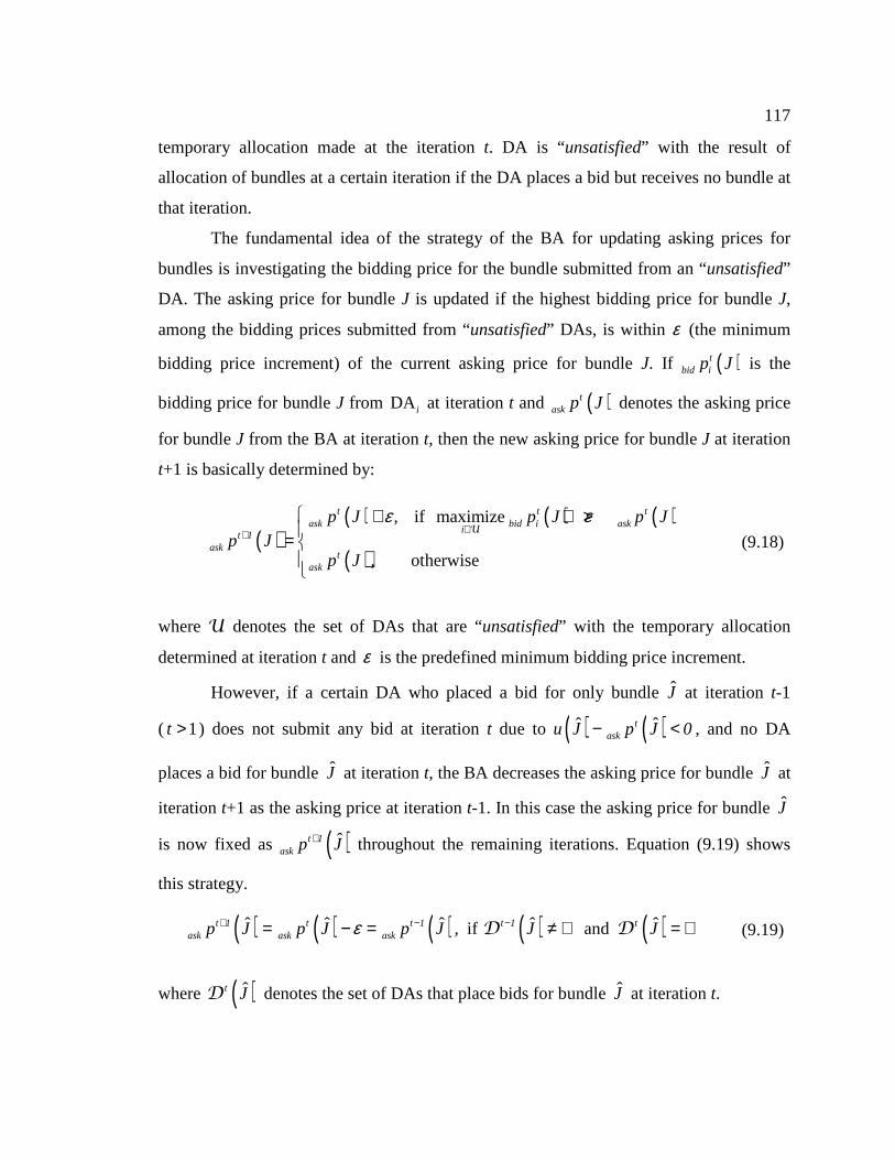
117

temporary allocation made at the iteration t. DA is “unsatisfied” with the result of

allocation of bundles at a certain iteration if the DA places a bid but receives no bundle at

that iteration.

The fundamental idea of the strategy of the BA for updating asking prices for

bundles is investigating the bidding price for the bundle submitted from an “unsatisfied”

DA. The asking price for bundle J is updated if the highest bidding price for bundle J,

among the bidding prices submitted from “unsatisfied” DAs, is within ε (the minimum

bidding price increment) of the current asking price for bundle J. If ( )tbid ip J is the

bidding price for bundle J from DA i at iteration t and ( )task p J denotes the asking price

for bundle J from the BA at iteration t, then the new asking price for bundle J at iteration

t+1 is basically determined by:

where U denotes the set of DAs that are “unsatisfied” with the temporary allocation

determined at iteration t and ε is the predefined minimum bidding price increment.

However, if a certain DA who placed a bid for only bundle J at iteration t-1

( 1t > ) does not submit any bid at iteration t due to ( ) ( )ˆ ˆtasku J p J 0− < , and no DA

places a bid for bundle J at iteration t, the BA decreases the asking price for bundle J at

iteration t+1 as the asking price at iteration t-1. In this case the asking price for bundle J

is now fixed as ( )ˆt 1ask p J+ throughout the remaining iterations. Equation (9.19) shows

this strategy.

where ( )ˆt JD denotes the set of DAs that place bids for bundle J at iteration t.

( )( ) ( ) ( )

( )

, if maximize

, otherwise

t t task bid i ask

it 1

askt

ask

p J p J p Jp J

p J

ε ε∈+

+ + >=

U

(9.18)

( ) ( ) ( ) ( ) ( )ˆ ˆ ˆ ˆ ˆ, if and t 1 t t 1 t 1 task ask askp J p J p J J Jε+ − −= − = ≠ ∅ = ∅D D (9.19)

118

From the above asking price strategy, it is always guaranteed that the DA having

the highest utility value for a certain bundle, among all the DAs, is automatically reserved

for the winner determination processes in the auction market.

Finally the BA’s asking price strategy not only enables the BA to increase its

revenue by reserving any DA submitting the highest bidding prices, but also provides a

DA with the second chance to obtain a bundle at the DA’s maximum bidding price by

decreasing the asking price for the bundle. Therefore, it is clear that the BA’s asking

price strategy encourages the proposed auction mechanism to promise allocative

efficiency in the auction market.

9.1.7 Example of Iterative Bundle Auction

This section presents a small size example of the proposed iterative bundle

auction mechanism for the first round local auction market. Suppose there are three

dealer agents, DA1, DA2, and DA3, in the market. The number of vehicles each DA has

and value of each bundle for DAs are given in Table 9.5. In this example the number of

available items (vacancies on a truck) is three.

Table 9.5: The number of vehicles and a value of each bundle.

Dealer agent The number of

vehicles

Value of bundle J

|J| = 1 |J| = 2 |J| = 3

DA1 1 20 20 20

DA2 2 0 50 50

DA3 3 0 0 60

Table 9.6 records the asking prices, bids placed from the DAs, and the temporal

allocation at each iteration of the iterative bundle auction mechanism where DAs place

XOR bids. In this example, minimum bidding price increment ε is set at 10. For each

iteration, the table records: (1) the asking prices for bundles at the beginning of the

iteration, (2) the XOR bids placed by the DAs, and (3) the result of temporal allocation

with the corresponding revenue for BA at the end of the iteration. The bids that maximize

119

the BA’s revenue are determined by solving the winner determination problem (indicated

with *).

In this example, the auction terminates at the end of iteration 13 where all DAs

are “satisfied” with the result of the temporary allocation of bundles. Thus, the allocation

of bundles at iteration 13, {[DA1, 1], [DA2, 2]}, becomes the final allocation. This

represents that a bundle, including one item, 1J = , is sold (allocated) to DA1 at the price

( ) 20p J = , and a bundle, including two items, 2J = , is sold to DA2 at the price

( ) 50p J = . Finally the BA’s revenue is equal to 70.

Table 9.6: Example of the iterative bundle auction mechanism: For the first round local auction market, where minimum bidding price increment ε is 10.

Asking price for |J| XOR Bid : ( |J|, bidding price for J ) Iteration

1 2 3 DA 1 DA2 DA3

Temporary allocation

Revenue

1 0 0 0 (1, 0) (2, 0) (3, 0) (2, 0) (3, 0) (3, 0)* [DA 3, 3] 0

2 10 10 10 (1, 10)* (2, 10) (3, 10) (2, 10)* (3, 10) (3, 0) [DA 1,1] [DA 2, 2] 20

3 10 10 10 (1, 10)* (2, 10) (3, 10) (2, 10)* (3, 10) (3, 10) [DA 1,1] [DA 2, 2] 20

4 10 10 20 (1, 10)* (2, 10) (3, 10) (2, 10)* (3, 10) (3, 20) [DA 1,1] [DA 2, 2] 20

5 10 10 30 (1, 10) (2, 10) (3, 10) (2, 10) (3, 10) (3, 30)* [DA 3, 3] 30

6 20 20 30 (1, 20)* (2, 20) (2, 20)* (3, 30) (3, 30) [DA 1,1] [DA 2, 2] 40

7 20 20 40 (1, 20)* (2, 20) (2, 20)* (3, 30) (3, 40) [DA 1,1] [DA 2, 2] 40

8 20 20 50 (1, 20) (2, 20) (2, 20) (3, 30) (3, 50)* [DA 3, 3] 50

9 30 30 50 StayA (2, 30) (3, 50)* [DA 3, 3] 50

10 20B 40 50 (1, 20)* (2, 40)* (3, 50) [DA 1,1] [DA 2, 2] 60

11 20 40 60 (1, 20) (2, 40) (3, 60)* [DA 3, 3] 60

12 20 50 60 (1, 20)* (2, 50)* (3, 60) [DA 1,1] [DA 2, 2] 70

13C 20 50 70 (1, 20)* (2, 50)* Stay [DA 1,1] [DA 2, 2] 70

A. Since the asking price for J is greater than the utility value of DA1 for J, the DA1 stays in the market (become “stay” state)

to see if the asking price drops in the next iteration.

B. Since no DA places a bid for the bundle J (|J| =1) at iteration 10, the BA decreases the asking price of J to the price at

iteration 9.

C. Since all DAs are “satisfied” with the result of the temporary allocation, the auction terminates. (By definition, a DA that

is in a “stay” state is always “satisfied” )

9.2 Design of Utility Function for Dealer Agent

Once a DA receives a request for bid (RFB) message from the BA, the DA

prepares an XOR bid by determining utility values of the bundles. Through the first round

local auction market, a DA seeks to achieve a bundle of vacancies on a truck in order to

ship the set of vehicles the DA has. For that reason, determination of the utility value of a

bundle of vacancies for a DA is based on the value of the set of vehicles the DA currently

has.

In the multiagent architecture for the shipment load makeup decision, the YA

provides a BA with cost information regarding the shipment yard, such as, holding costs

and re-processing costs. The RM also provides a BA with the arrival time of the next

truck. Finally, each BA provides this cost and operational information to the

corresponding DAs through an RFB message. The utility value of a bundle for a DA is

computed by information provided thorough the RFB message as well as the DA’s local

information.

A dealer agent i, DA i , computes the value for the set of vehicles, iV , using the

DA’s local information and the information provided by the RFB message from the BA.

If ∆ ( t t∆ = −% ) is the discrete time interval between the current time t and the arrival

time of the next truck t% , then the value of iV for DA i , ( )i iv V , is represented as:

where ( )Si iv V and ( )D

i iv V denote the values of iV in the shipment yard and local

dealer i, respectively. The values of iV in the shipment yard and local dealer i are

defined as:

( ) ( ) ( )S Di i i i i iv v v= +V V V (9.20)

( ) ( ) ( )i

S HD RPi i

v

v C v C v∆ ∆∈

= + ∑V

V (9.21)

( ) ( ) ( )i

D DL LTi i

v

v C v C v∆ ∆∈

= + ∑V

V (9.22)

122

From the above definitions, clearly ( )i iv V implies the total inevitable cost

created since the set of vehicles for DA i is not shipped by the truck at time t. As

represented in Equation (9.20), the total inevitable cost is calculated by subtracting a

fixed visiting and unloading cost for dealer i from the sum of the costs created by the

shipment yard and local dealer i during the time interval∆ . Finally a utility value of

bundle J for DA i is defined as:

9.3 The Second Round Central Auction

Once the set of winning DAs is determined from each first round local auction

market, the winning DAs proceed to the second round central auction market. In the

second round central auction market, the winning DAs in the same block do not compete

with each other any more, but they cooperate with each other to achieve their common

goals to obtain all the vacancies on the truck by competing with other sets of DAs

determined from other blocks, i.e., other first round local auction markets. In other words,

a competition occurs among different sets of DAs. To this end, instead, the set of winning

DAs joins directly the second round central auction market, a BA participates in the

auction market as a proxy agent who is in charge of representing the set of winning DAs

in its block, and the BA competes with other BAs to achieve all the vacancies on the

truck. Thus, the role of the second round central auction market is to allocate all the

vacancies on the truck to one of BAs in order to maximize the revenue for the RA (seller)

and the profit values for BAs (buyers) in the market.

9.3.1 Structure of the Second Round Central Auction Market

( ) ( ) , if

, otherwise

i i i

i

v Ju J

0

≥=

V V (9.23)

123

Once every BA is ready to join the second round central auction market by

determining the set of winning DAs in its own first round local auction market, the RM

sends an RFB message to BAs to initiate the auction market. Through the RFB message,

the RM requests every BA to respond to the RM. The response from each BA includes an

operational requirement for delivery, such as information on the set of winning DAs

(dealers needed to visit) and the total number of vehicles included in the winning DAs

(the total number of required vacancies). Based on the response, the RM determines an

operational cost of the RA (the truck) for each BA, meaning that the RA has a different

operational cost for every BA. For example, the operational cost of truck r for BA i ,

( )ic r , is computed by:

where BA is the set of BAs joining the auction market and iW denotes the set of

winning DAs for BA i . In this equation, jJ denotes the size of the bundle jJ finally

allocated to DA j from the result of the first round local auction market. Thus jJ

implies the number of vehicles included in DA j .

Once the RM determines operational costs for all BAs, the RM sends this

information to the RA. Figure 9.5 shows the structure of the second round central auction

market.

( ) , for i i

TR UL URi i ij j

j j

c r C C J C iΨ∈ ∈

= + + − ⋅ ∀ ∈

∑ ∑W W

BA (9.24)

124

Fig. 9.5: Structure of the second round central auction market.

The fundamental process of the second round auction mechanism follows the

ascending price iterative auction mechanism, introduced in Chapter 6. However, the

second round auction mechanism allows the RA (seller) to adopt different asking prices

for BAs (buyers) in order to consider the different operational costs for BAs.

9.3.2 Utility Value for Block Agent

In the second round central auction market, the utility value of truck r for BA i ,

( )BAiu r , is computed by following Equation (9.25), where iW denotes the set of winning

DAs in the first round local auction market for block i, Mst1

i , and ( )j ju J , defined in

Section 8.2, is the utility value of bundle jJ for DA j that was finally allocated to DA j

from the result of the first round local auction market.

BA

RM

BA (Buyers)

RFB message

BA

BA

BA

Second Round Central Auction Market

RA

RA

RA

RA

RA

RA (Seller)

Operational requirement

125

In the second round central auction market, the profit value of truck r for BA i is a

difference between the utility value and the price, ( ) ( )BAiu r p r− .

9.3.3 Block Agent Bidding Strategy

An auction mechanism for the second round central auction market proceeds in

iterations starting with initial asking prices and random allocations. An initial asking

price the RA offers to every BA is set at zero. Each iteration starts with the temporary

allocation of the truck, determined at the end of previous iteration, and a set of asking

prices for BAs.

In each iteration, if any BA is not “satisfied” with the temporary allocation

determined at the previous iteration, this BA submits a bidding price to achieve the truck.

In this auction market, BA i would be “satisfied” with the allocation if BA i achieves

space on the truck or if the profit value of truck r is less than or equal to ε as shown in

Equation (9.26).

Once BA i who is not “satisfied” with the temporary allocation, BA i submits a

bidding price, ( )bid ip r , to obtain space on the truck. The bidding strategy used in this

auction market allows a BA to submit the bidding price that is equal to the asking price

offered from the RA so that a bidding price is set as low as possible.

9.3.4 Updating Temporary Allocation

( ) ( )BA

i

i j jj

u r u J∈

= ∑W

(9.25)

( ) ( )BAi ask iu r p r ε− ≤ (9.26)

126

If any BA i submits a bidding price, ( )bid ip r , the RA updates the current

allocation of the truck so as to increase the revenue. The RA now takes the truck from the

BA to which the truck was originally allocated at the beginning of the iteration, and then,

allocates the truck to BA i .

9.3.5 Updating Asking Price for Truck

If BA i receives the truck at the end of iteration t by placing bidding price

( )tbid ip r that is equal to ( )t

ask ip r , the RA sets the price for the truck, ( )tp r , to ( )tbid ip r ,

and updates asking prices to other BAs except BA i at the next iteration t+1. A new

asking price to each BA is determined as:

where ( )ic r and ( )jc r denote the operational cost of truck r for BA i and BA j ,

respectively. By this definition of updating asking prices, the RA’s revenue increment is

always equal to ε .

9.3.6 Market Termination

Figure 9.6 shows the overall procedure of the auction mechanism in the second

round central auction market. As shown in this figure, the auction proceeds in a sequence

of iterations until all BAs are “satisfied” with the allocation results. If all BAs are

“satisfied” with the temporary allocation determined at a certain iteration, the second

round central auction market terminates promptly by settling this result as the final

allocation.

( ) ( ) ( ) ( ) { }, for \t 1 task j ask i i jp r p r c r c r j iε+ = − + + ∀ ∈ BA (9.27)

127

Fig. 9.6: The overall procedure of the auction mechanism in the second round central auction market.

Open the second round central auction market

Initial allocation and asking prices to BAs

set t = 0

t = t + 1

Are all BAs “satisfied” with temporary

allocation?

The auction market terminates

set i = 0

Is BAi

“satisfied” with temporary allocation?

Submit bidding price ( )tbid ip r

Update temporary allocation

Update asking prices for

( ) ( ) ( ) ( )t 1 task j ask i i jp r p r c r c r ε+ = − + +

i = i + 1

NO

YES

NO

YES

{ }\j i∀ ∈BA

128

Chapter 10

Shipment Load Makeup – Solution Methodology Part III

For the RFID-enabled shipment load makeup decision in Scenario 2, explained in

Section 8.2.2, this study proposes the single-tier auctioning process which facilitates

multiple direct local auction markets. This chapter presents the single-tier auctioning

process by detailing a market organization and an auction mechanism for a direct local

auction market.

10.1 Dealer Agent in Single-Tier Auctioning Process

The fundamental ideas in designing the single-tier auctioning process are from

consideration of enhanced abilities of a dealer agent (DA) in a mulitagent-based auction

market. Compared to DAs in the two-tier auctioning process, explained in Chapter 9, the

DAs in the single-tier auctioning process are regarded to have the following

communicational and computational abilities:

� A DA is able to negotiate for items (vacancies on a truck) directly with a resource

agent (RA). This direct negotiation procedure enables a DA to obtain a part of the

RA’s local information through the advanced communication during an

auctioning process.

� A DA has an advanced computational ability for individually controlling the

vehicles included in the DA. This enables a DA to place a bid to obtain a single

item (a single vacancy) for each individual vehicle during an auctioning process.

10.2 Construction of the Direct Local Auction Market

129

Once a truck arrives at the shipment yard to load vehicles, i.e., one of RAs

becomes available, the RM informs the MC of the availability of the RA. Now, the MC

initiates a temporary economy for direct local auction markets. The design of the single-

tier auctioning process requires defining a proxy agent (PA) class. A PA class agent is a

virtual entity for the market mechanism’s purpose, and the fundamental role of a PA class

agent is:

� Proxy Agent (PA): a PA class agent is responsible for establishing and

coordinating a direct local auction market on behalf of the RA, and the set of PAs

is { }PA |b b= ∈PA B . A PA, as a virtual seller, interacts with DAs (buyers) in a

direct local auction market.

In the temporary economy initiated by the MC, each PA establishes a direct local

auction market by sending an RFB message to each corresponding DA. The RFB

message for a DA includes the partial local information on the RA (the truck), such as the

visiting and unloading cost at the DA for the truck. Since a direct local auction market is

established for each block area, total B auction markets, where B is the number of block

areas, are constructed simultaneously. Figure 10.1 describes the construction of

temporary economy and multiple direct local auction markets.

130

Fig. 10.1: Construction of a temporary economy and multiple direct local auction markets.

In the single-tier auctioning process, each direct local auction market proceeds

independently to determine the set of provisional winning vehicles by virtually allocating

vacancies on the truck to the vehicles included in DAs.

The design of an auction mechanism for each direct local auction market is an

iterative high-bid auction mechanism, which is basically a type of first-price sealed-bid

auction mechanism7. The designed auction mechanism is applied independently to all the

direct local auction markets. This chapter presents the iterative high-bid auction

7 A first-price sealed-bid auction mechanism is also known as sealed high-bid auction mechanism or sealed-bid first-price auction mechanism. In this type of auction, potential bidders (buyers) simultaneously place sealed bids so that no bidder knows the bid of any other participant. The highest bidder is awarded the item at the price he or she placed (McAfee and McMillan, 1987).

DA

Direct local auction market for block 1

DA


RM

RA’s local information

RA

RA

RA

RA

MC

PA

DA

DA

DA


RFB

RFB

RFB

RA

PA

PA

Temporary Economy

131

mechanism by detailing the auctioning process in a certain direct local auction market

M DLb ( )b ∈B . Let G be the set of vacancies on the truck, and bD represents the set of

DAs participating in the direct local auction market for block area b, M DLb . As a matter of

convenience in representing the index, D and M DL are used rather than bD and M 1stb in

this chapter8.

10.3 Iterative High-Bid Auction Mechanism

At each iteration, a single item (a vacancy) is allocated to a DA. Thus, each

iteration implies an auction market for a single item, and the number of iterations

required is always less than or equal to the number of available items (the number of

available vacancies on the truck). On behalf of the RA, the PA plays an auctioneer as

well as a seller who controls the direct local auction market. Each iteration is initiated by

sending RFB messages to DAs. The RFB message for a DA includes announcement of

the availability of an item, the partial local information on the RA, such as the visiting

and unloading cost related to the DA, and the allocation result of the previous iteration.

Once a DA receives an RFB message, the DA decides whether to place a bid or not. If a

DA decides to place a bid, the DA submits a bidding price for the item. By receiving all

of the bids from DAs, the PA determines an allocation of the item. Based on the result of

the allocation, if required, each DA updates the bidding price at the beginning of next

iteration. The auction market terminates when all available items are allocated to DAs or

no DA places a bid for an item. The overall procedure of the iterative high-bid auction

mechanism appears in Figure 10.2.

8 Since each direct local auction market proceeds independently with the same auction mechanism, the auction mechanism is presented in the domain of a certain direct local auction market, and the block index b (b∈B) is omitted for the convenience of mathematical presentation.

132

Fig. 10.2: Overall procedure of the iterative high-bid auction mechanism.

10.3.1 Dealer Agent Bidding Strategy

A DA is designed to request a single vacancy on a truck to load one of available

vehicles the DA has. Vacancies on a truck are items allocated to DAs through an auction

market. In the iterative high-bid auction mechanism, a DA places a bid by submitting a

bidding price for an item to the PA., and the bidding price is basically determined by the

utility value of the item for the DA. Let tbid ip be the bidding price of dealer agent i, DA i ,

at iteration t, which is represented as:

ULt t i

bid i i ti

Cp u

1λ= −

+ (10.1)

Iteration 1

Initiate auction market

Request for bids

Place bids

Allocation

Market termination

Yes

Close auction market

Place bids

Allocation

Yes

Request for bids

Update bidding prices

Place bids

Allocation

Yes

Request for bids

Update bidding prices

Iteration 2 Iteration 3

Close auction market Close auction market

Market termination

Market termination

133

where tiu denotes the utility value of an item for DA i at iteration t, UL

iC is the visiting

and unloading cost at DA i , and tiλ represents the number of items DA i has obtained

before iteration t 9. This definition guarantees that: (1) the visiting and unloading cost at

DA i is distributed to the items allocated to DA i , and (2) a DA that has obtained more

items through the previous iterations has more chance to obtain an item by submitting a

higher bidding price for the item. This also enables a truck to reduce its operational cost

for deliveries by reducing the number of dealers the truck needs to visit for unloading

vehicles.

10.3.2 Utility Value for Dealer Agent

Once a DA receives an RFB message from the PA, the DA prepares a bid by

determining a bidding price. As defined in Equation (10.1), a bidding price of a DA is

determined based on the utility value of an item for the DA. Through the auction market,

a DA seeks to achieve items representing vacancies on the truck in order to ship vehicles.

For that reason, the utility value of an item for a DA is defined by the value of the vehicle

the DA has.

At the beginning of the first iteration for the direct local auction market, a DA

determines a value of each vehicle the DA currently has using information provided by

the RFB message from the PA, as well as the DA’s local information. If ( )v j is the

value of vehicle j for a DA, then ( )v j is defined as:

where ( )Sv j and ( )Dv j denote the values of vehicle j in the shipment yard and the

dealer that orders vehicle j, respectively, and they are defined as:

9 By this definition, the value of tiλ for all DAs is set to 0 at the first iteration (t=1).

( ) ( ) ( )S Dv j v j v j= + (10.2)

134

From the above definition, it is clear that ( )v j implies the sum of the costs

arising from the shipment yard and the dealer that orders vehicle j during the time

interval ∆ 10 because vehicle j is not shipped by the truck.

In order to set a bidding price as high as possible at every iteration, a DA looks

for the vehicle having the highest value among all the vehicles the DA has. This implies

that a DA places a bid for an item so as to assign the item, if the DA obtains the item, to

the vehicle having the highest value. Finally, the utility value of an item for DA i at

iteration t, tiu , is defined as:

where tiV is the set of available vehicles for DA i at iteration t. For all iterations t except

the first iteration( )1i i=V V , t

iV is defined as:

In the above equation, tij% is the vehicle that has the highest value among the

vehicles included in DA i at iteration t, that is, ( ){ }arg maxt

i

ti

j

j v j∈

=V

% .

10.3.3 Winner Determination at Each Iteration

10 As defined in Chapter 8, ∆ ( t t∆ = −% ) is the discrete time interval between the current time t and the arrival time of the next truck t% .

( ) ( ) ( )S HD RPv j C j C j∆ ∆= + (10.3)

( ) ( ) ( )D DL LTv j C j C j∆ ∆= + (10.4)

( ){ }maxt

i

ti

ju v j

∈=

V (10.5)

{ }\ , if DA obtained an item at iteration -1

, otherwise

t 1 t 1i i i

ti

t 1i

j t− −

−

=

VV

V

%

(10.6)

135

At the end of every iteration, the PA determines an allocation of an item to one of

the DAs who placed bids. In the iterative high-bid auction mechanism, the PA allocates

an item to the DA who submitted the highest bidding price. For instance, the winning DA

awarded an item at iteration t is determined by:

where tD denotes the set of DAs that place bids at iteration t.

10.3.4 Revenue of PA from Auction Market

Once the auction market terminates, the PA informs the RA of the result of the

auction market. The result of the auction market is represented as a form of

* *, ,PAr DA J , where PAr denotes the revenue of the PA from the auction market,

*DA denotes the set of DAs obtaining any item from the auction market, and *J

denotes the set of vehicles to which each DA in *DA assigns its obtained item(s). The

revenue of the PA from the auction market, PAr , is computed by:

10.3.5 Example of Iterative High-Bid Auction

This section presents a small size example of the iterative high-bid auction

mechanism. For the example, four dealer agents, DA1, DA2, DA3, and DA4, are populated

in the market. The fixed cost for visiting and unloading and the values of vehicles for

each DA appear in Table 10.1. In this case the number of available items (vacancies on

the truck) is seven.

{ }*

DA

DA arg maxt

i

t tbid ii

p∈

=D

(10.7)

( )* *

ULPA i

j i

r v j C∈ ∈

= −∑ ∑J DA

(10.8)

136

Table 10.1: The fixed cost for visiting and unloading and the values of vehicles.

Dealer agent Fixed cost for visiting

and unloading Vehicle Value of vehicle

DA1 30

j11 25

j12 2

j13 1

DA2 20 j21 10

j22 14

DA3 24 j31 6

j32 4

DA4 28

j31 12

j32 16

j33 18

Table 10.2 records the bidding prices submitted from DAs, where the highest

bidding price is indicated with *, and the results of allocations at each iteration of the

iterative high-bid auction mechanism. For instance, at iteration 1, the PA allocates an

item to DA1 who submitted the highest bidding price, equal to -5, and DA1 assigns the

item to vehicle j11 which has the highest value, 25, among all the vehicles DA1 has. In

this example, the auction terminates at the end of iteration 7 with allocation of the last

item. The final result of allocations is {[DA1, j11, j12], [DA2, j21, j22] , [DA4, j41, j42, j43]},

which represents that DA1 achieves two items for vehicle j11 and j12, DA2 obtains two

items for vehicle j21 and j22, and DA4 achieves three items for vehicle j41, j42, and j43. In

this example, *J and *DA are { j11, j12, j21, j22, j41, j42, j43} and {DA1, DA2, DA4},

respectively, and the revenue for the PA from the auction market is:

( ) ( ) ( ) ( ) ( ) ( ) ( ){ }{ }

{ } { }

25+2+10+14+12+16+18 30+20+28 9

PA 11 12 21 22 41 42 43

UL UL UL1 2 4

r v j v j v j v j v j v j v j

C C C

= + + + + + +

− + +

= − =

Table 10.2: Small size example of the iterative high-bid auction mechanism.

Bidding price of DAi Iteration

DA 1 DA2 DA3 DA4 Allocation

1 max {25, 2, 1} - 30 = -5* max {10, 14} - 20 = -6 max {6, 4} - 24 = -18 max {12, 16, 8} - 28 = -12 [DA1, j11]

2 max {2, 1} - 15 = -13 max {10, 14} - 20 = -6* max {6, 4} - 24 = -18 max {12, 16, 8} - 28 = -12 [DA2, j22]

3 max {2, 1} - 15 = -13 max {10} - 10 = 0* max {6, 4} - 24 = -18 max {12, 16, 8} - 28 = -12 [DA2, j21]

4 max {2, 1} - 15 = -13 - max {6, 4} - 24 = -18 max {12, 16, 8} - 28 = -12* [DA4, j42]

5 max {2, 1} - 15 = -13 - max {6, 4} - 24 = -18 max {12, 8} - 14 = -2* [DA4, j41]

6 max {2, 1} - 15 = -13 - max {6, 4} - 24 = -18 max {8} – 9.33 = -1.33* [DA4, j43]

7 max {2, 1} - 15 = -13* - max {6, 4} - 24 = -18 - [DA 1, j12]

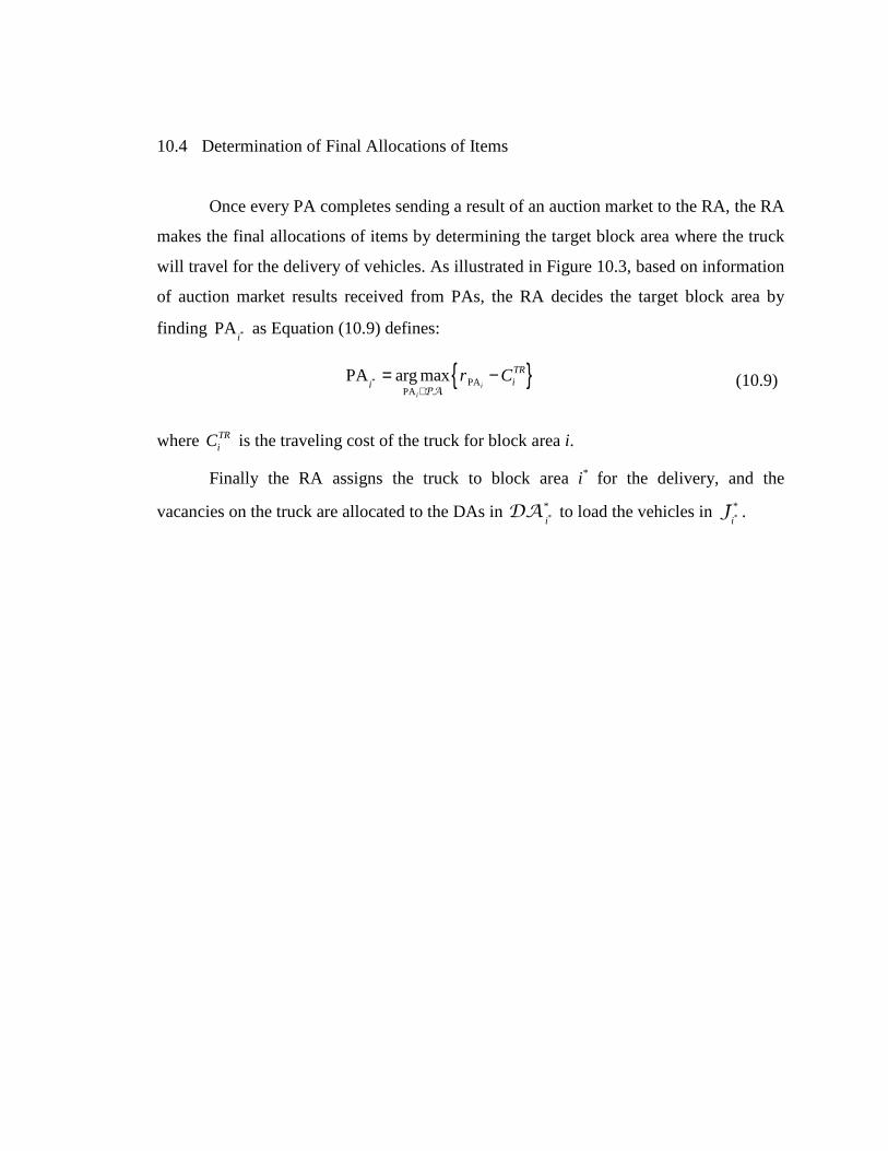
10.4 Determination of Final Allocations of Items

Once every PA completes sending a result of an auction market to the RA, the RA

makes the final allocations of items by determining the target block area where the truck

will travel for the delivery of vehicles. As illustrated in Figure 10.3, based on information

of auction market results received from PAs, the RA decides the target block area by

finding *PAi

as Equation (10.9) defines:

where TRiC is the traveling cost of the truck for block area i.

Finally the RA assigns the truck to block area *i for the delivery, and the

vacancies on the truck are allocated to the DAs in *

*

iDA to load the vehicles in *

*

iJ .

{ }* PAPA

PA arg maxi

i

TRii

r C∈

= −PA

(10.9)

139

Fig. 10.3: RA’s final allocations determined by results of all the local auction markets.

PA1 Auction market result

DA DA DA RA PA i*

PAB

**iJ

**iDA

DA DA DA

*1J

*1DA

DA DA DA

*1J

*1DA

Result of auction market i (block area i)

* *PA , ,

1 1 1r DA J

Result of auction market B (block area B)

Result of auction market 1 (block area 1)

140

Chapter 11

Empirical Analysis of Shipment Load Makeup

Experimental analysis and validation of the proposed approaches is important part

of this research. However, testing and verifying the proposed approaches in a real

shipment load makeup environment is very difficult due to large scale and variety of

functional entities and managerial information in that environment. Thus, thorough

testing and analysis is conducted in an experimental setting using a variety of shipment

load makeup instances. In order to conduct experimental analysis, a simulator, which

emulates shipment load makeup processes with the proposed auction mechanisms, is

developed. This chapter presents the experimental setup and shipment load makeup

instance generation followed by the experimental analysis results. The experimental

analysis results demonstrate the proposed approaches accomplish high level of solution

quality and computational efficiency.

11.1 Experimental Setup

11.1.1 Simulator for Shipment Load Makeup

This study develops and uses a simulator for a comprehensive experimental

analysis of shipment load makeup processes with various auction mechanisms. As shown

in Figure 11.1, the structure of the simulator primarily consists of three program

components: problem instance generator, centralized planner, and market-based

decentralized planner.

141

Fig. 11.1: Structure of shipment load makeup simulator.

� Problem instance generator: This program component generates a variety of

shipment load makeup instances using input parameters given by users. For each

shipment load makeup instance, the problem instance generator also creates an IP

formulation of the instance, which is based on the centralized IP formulation

explained in Sections 8.2.1 and 8.2.2.

Problem Instance Generator

Centralized Planner

Market-based Decentralized Planner

Local market 1

Compare & Validate

Input parameters

s

LINDO Two-tier

auctioning Single-tier auctioning

Auction mechanism

Auction mechanism

Scenario 1 Scenario 2

Local market 2

Local market n

142

� Centralized planner: A centralized planner component uses LINDO (Linear

Interactive Discrete Optimizer)11 to generate optimal solutions of shipment load

makeup instances. An IP formulation generated from the problem instance

generator is used as a LINDO input model. Figures 11.2 and 11.3 show examples

of LINDO input generated for a small-size shipment load makeup instance.

� Market-based decentralized planner: A market-based decentralized planner

component is further decomposed into two sub-components, such as two-tier

auctioning process (explained in Chapter 9) and single-tier auctioning process

(explained in Chapter 10), which are designed for different shipment load makeup

scenarios. The developed auction mechanisms for local auction market are

embedded in corresponding sub-components to manipulate shipment load makeup

instances in a decentralized manner and to provide solutions of the instances.

Fig. 11.2: Example of LINDO input for Scenario 1, which is automatically generated by problem instance generator (5 blocks, 5 dealers per block, and 50 vehicles).

11 LINDO is an interactive linear, quadratic, and integer programming package, http://www.lindo.com/

143

Fig. 11.3: Example of LINDO input Scenario 2, which is automatically generated by problem instance generator (5 blocks, 5 dealers per block, and 50 vehicles).

11.1.2 Generation of Shipment Load Makeup Instances

For the intensive computational experiments and analysis, a variety of different

shipment load makeup instances are generated by defining various input parameters in

the shipment load makeup environment. About twenty-five parameters are defined in the

144

input file by users to generate shipment load makeup instances. These input parameters

are divided by two categories: configuration-related parameter group and cost-related

parameter group. Tables 11.1 and 11.2 summarize the important input parameters to be

controlled for generating shipment load makeup problem instances.

Table 11.1: Controllable shipment load makeup configuration parameter.

Parameter Description

SLMsce INDIV: shipment load makeup scenario 1(Section 8.2.1) DIV: shipment load makeup scenario 2 (Section 8.2.2)

B number of blocks

Dmin minimum number of dealers in a block

Dmax maximum number of dealers in a block

V number of available vehicles in a shipment yard

Ψ capacity (number of vacancies) of a truck

∆ length of discrete time till arrival of the next truck

L maximum allowed dwell time for a vehicle

α dwell time control parameter

SCmin minimum shipment commitment time for a vehicle

SCmax maximum shipment commitment time for a vehicle

From the input parameters, Dmin and Dmax, listed in Table 11.1, the number of

dealers in a certain block b, Db, is randomly generated from a uniform distribution on the

interval [Dmin, Dmax].

145

Table 11.2: Controllable shipment load makeup cost parameter.

Category Parameter Description

Shipment yard

m vehicle holding cost parameter 1

n vehicle holding cost parameter 2

crp re-processing cost for a vehicle

Dealer

pmin minimum delayed order cost parameter 1

pmax maximum delayed order cost parameter 1

qmin minimum delayed order cost parameter 2

qmax maximum delayed order cost parameter 2

cltmin minimum lost order cost

cltmax maximum lost order cost

Truck

CTRmin minimum traveling cost to a block

CTRmax maximum traveling cost to a block

CULmin minimum visiting and unloading cost at a dealer

CULmax maximum visiting and unloading cost at a dealer

CUR unutilized capacity cost per vacancy

Among the parameters listed in Table 11.2, the following parameters need to be

explained in a little bit more:

� Holding cost parameters (m and n), are used to define a holding cost for time

period [l-1. l], ( )hdc l , which is a monotonically increasing function as explained

in Section 3.4.2. For the experimental analysis, this study uses a simple linear

increasing function, such as ( )hdc l m n l= + ⋅ .

� Delayed order cost parameters (pmin, pmax, qmin, and qmax), are used to define a

delayed order cost for vehicle v for time period [l-1. l], ( )dlvc l , explained in

Section 3.4.2. Similar to a holding cost, a simple linear increasing function is used

for each vehicle, such as ( )dlv v vc l p q l= + ⋅ . For each vehicle, the cost parameters,

146

pv and qv, are randomly generated from uniform distributions on the intervals

[pmin, pmax] and [qmin, qmax], respectively.

Using the input parameters, the problem instance generator creates the vehicles

currently available for the shipment load makeup, and values of vehicle attributes are

randomly generated, as described in Table 11.3.

Table 11.3: Random generation of vehicles in a shipment yard.

Attribute Description Value

bv block area for vehicle v uniform [1, B]

dv dealer for vehicle v uniform [1, Db]

lv dwell time for vehicle v uniform [1, DTmax]

ωv shipment commitment time for vehicle v uniform [SCmin, SCmax]

cltv lost order cost for vehicle v uniform [clt

min, clt

max]

pv delayed order cost parameter 1 for vehicle v uniform [pmin, pmax]

qv delayed order cost parameter 2 for vehicle v uniform [qmin, qmax]

The dwell time for each vehicle is randomly generated from a uniform

distribution on the interval [1, DTmax], where upper bound of dwell time, DTmax, is

defined as:

As the value of over-dwell control parameter, α, increases, the number of over-

dwelled vehicles, whose dwell time will exceed the maximum allowed dwell time, L,

during the time interval, ∆, also increases.

11.2 Performance of Market-based Approach for Shipment Load Makeup

In order to test the solution optimality and computational efficiency of the

proposed market-based approach, total 40 small-size shipment load makeup instances (5

maxDT Lα∆= − (11.1)

147

block areas) are investigated. For each of these shipment load makeup instances, a total

of 5 simulation runs are repeated to reduce random effects. The input parameters used for

generating these instances are shown in Table 11.4, and, for the experimentations of the

two-tier auctioning process, the minimal bidding increment (ε) is set to 100.

Table 11.4: Input parameters values used for generating shipment load makeup instances.

Parameter Value Parameter Value Parameter Value

Ψ 12 m 0.05 cltmin 80.0

∆ 20 n 0.005 cltmax 120.0

L 150 crp 80.0 CTRmin 500.0

α 1.5 pmin 0.05 CTRmax 800.0

SCmin 15 pmax 0.15 CULmin 100.0

SCmax 120 qmin 0.02 CULmax 200.0

qmax 0.04 CUR 100.0

11.2.1 Performance of Two-tier Auctioning Process for Scenario 1

Table 11.6 and Figures 11.4 and 11.5 summarize the experimental results of the

two-tier auctioning process for shipment load makeup scenario 1, where the vehicles in

the same dealer are not divisible during shipment load makeup process. In this result

table, each column name is described as shown in Table 11.5.

148

Table 11.5: Description of each column in the experiment result table.

Column name Description

No_B number of block areas

ANo_D average number of dealers per block

TNo_D total number of dealers

ANo_V average number of vehicle per dealer

TNo_V total number of vehicles

OptSol optimal solution obtained from LINDO

CompT computational time (second) in LINDO

M_Sol solution obtained from the proposed market-based approach

M_CompT computation time (second) in the proposed market-based approach

%Opt optimality of the proposed market-based approach (optimal = 1.0)

%Eff computational efficiency factor of the proposed market-based

approach (= M_CompT / CompT)

As shown in Figure 11.4, the optimality of the solution is very high, ranging

93.2% to 99.9% of the optimal solution, which generated by LINDO, while the average

computation time is about 45.5% of the LINDO solution. Figure 11.5 illustrates the

computational efficiency of the two-tier auctioning process. As shown in this figure, the

average value of computational efficiency factor, %Eff = M_CompT / CompT, decreases

almost linearly as the average number of dealers per block increases. In shipment load

makeup scenario 1, the computation time for both approaches is significantly dependent

on the average number of dealers per block. Especially for the IP formulation, the number

of integer variables increases rapidly, as the number of dealers increases. The difference

between computational times of the two-tier auctioning process and a centralized

approach using the IP formulation will become bigger when the two-tier auctioning

process is implemented in a multiagent system, where multiple local auction markets in

the two-tier auctioning process are to be processed by corresponding block agents

simultaneously in distributed local computers.

Table 11.6: Experimental results of the two-tier auctioning process for the shipment load makeup scenario 1.

No_B ANo_D TNo_D ANo_V TNo_V OptSol CompT M_Sol M_ComT %Opt %Eff

5 10 50

2 100 -1611.12 0.6 -1609.73 0.401 0.9992 0.668

4 200 -1724.96 0.6 -1713.39 0.425 0.9932 0.708

6 300 -1705.54 0.8 -1703.39 0.531 0.9987 0.664

8 400 -1910.89 0.6 -1894.31 0.517 0.9913 0.861

5 20 100

2 200 -1713.44 1.6 -1678.14 0.533 0.9794 0.333

4 400 -1949.84 1.4 -1920.01 0.749 0.9847 0.535

6 600 -1953.03 1.6 -1894.05 0.909 0.9698 0.568

8 800 -1856.54 1.8 -1818.48 1.186 0.9795 0.659

5 30 150

2 300 -1649.41 2.4 -1597.77 0.756 0.9647 0.311

4 600 -1998.77 2.6 -1961.52 1.087 0.9814 0.418

6 900 -1961.29 2.8 -1944.07 1.203 0.9921 0.430

8 1200 -2071.03 2.4 -2049.70 1.539 0.9897 0.641

5 40 200

2 400 -1952.75 3.4 -1864.29 0.843 0.9547 0.247

4 800 -1938.34 3.4 -1910.95 1.234 0.9859 0.363

6 1200 -2100.65 3.6 -2058.59 1.456 0.9799 0.404

8 1600 -2048.18 3.2 -1977.93 1.881 0.9657 0.589

5 50 250

2 500 -2195.19 5.8 -2148.94 0.937 0.9783 0.161

4 1000 -2088.11 5.2 -1946.56 1.998 0.9322 0.384

6 1500 -2170.99 6.2 -2105.75 2.015 0.9699 0.325

8 2000 -2112.91 5.8 -2075.17 2.556 0.9821 0.441

Fig. 11.4: Optimality of the two-tier auctioning process solution varying the average number of dealers per block and the average number of vehicles per dealer: (a) the average optimality, (b) ANo_D = 10, (c) ANo_D = 20, (d) ANo_D = 30, (e) ANo_D = 40, and (e) ANo_D = 50.

0

0.2

0.4

0.6

0.8

1

10 20 30 40 500

0.2

0.4

0.6

0.8

1

2 4 6 8

0

0.2

0.4

0.6

0.8

1

2 4 6 80

0.2

0.4

0.6

0.8

1

2 4 6 8

0

0.2

0.4

0.6

0.8

1

2 4 6 8

0

0.2

0.4

0.6

0.8

1

2 4 6 8

ANo_D (a) (b)

ANo_V

(c) (d)

(e) (f)

ANo_D = 10

ANo_D = 20 ANo_D = 30

ANo_D = 40 ANo_D = 50

151

Fig. 11.5: Computational efficiency of the two-tier auctioning process varying the average number of dealers per block.

11.2.2 Performance of Single-tier Auctioning Process for Scenario 2

Table 11.7 with Figures 11.6 and 11.7 shows the experimental results of the

single-tier auctioning process for scenario 2, where the vehicles in the same dealer can be

divisible during shipment load makeup process. As illustrated in Figure 11.6, the

optimality of the single-tier auctioning process solution is high, ranging 91.8% to 98.4%

of the optimal solution, while the average computation time of the single-tier auctioning

approach is only about 8.23% of the LINDO solution. Figure 11.7 shows the

computational efficiency of the single-tier auctioning process. As shown in this figure,

the average value of computational efficiency factor, %Eff, decreases almost

exponentially as the average number of vehicles per dealer increases. For shipment load

makeup scenario 2, the number of integer variables in the IP formulation increases

significantly, as the number of vehicles increases. Similar to the two-tier auctioning

process, the gap between computational efficiencies of the single-tier auctioning process

and the IP formulation approach will become larger if the auctioning process is

0

0.2

0.4

0.6

0.8

1

10 20 30 40 50

average number of dealers per block

average %Eff

152

implemented in a multiagent system, where each local auction market is to be processed

by corresponding proxy agent simultaneously in distributed local computers.

Table 11.7: Experimental results of the single-tier auctioning process for the shipment load makeup scenario 2.

No_B ANo_D TNo_D ANo_V TNo_V OptSol CompT M_Sol M_ComT %Opt %Eff

5 10 50

2 100 -1630.66 1.0 -1605.12 0.160 0.984 0.16

4 200 -2112.62 1.4 -1987.54 0.265 0.941 0.189

6 300 -2309.92 1.4 -2216.68 0.343 0.959 0.245

8 400 -2362.25 2.8 -2224.41 0.484 0.942 0.173

5 20 100

2 200 -1879.13 1.6 -1740.78 0.312 0.926 0.195

4 400 -2215.17 3.0 -2171.31 0.531 0.980 0.177

6 600 -2365.81 8.2 -2170.66 0.734 0.918 0.089

8 800 -2442.87 14.2 -2247.82 0.890 0.921 0.062

5 30 150

2 300 -1757.46 10.2 -1673.38 0.453 0.952 0.044

4 600 -2381.79 73.2 -2210.43 0.781 0.928 0.011

6 900 -2462.21 182.2 -2294.18 0.937 0.931 0.005

8 1200 -2534.36 359.6 -2337.84 1.125 0.922 0.003

5 40 200

2 400 -2050.08 18.2 -1926.73 0.484 0.941 0.027

4 800 -2178.34 136 -2043.51 1.015 0.938 0.007

6 1200 -2457.27 424 -2274.17 1.062 0.925 0.003

8 1600 † † -2520.59 1.703 † †

5 50 250

2 500 -2339.51 81.2 -2188.38 0.531 0.935 0.006

4 1000 -2396.94 467 -2203.85 1.296 0.919 0.002

6 1500 † † -2326.93 1.64 † †

8 2000 † † -2578.30 2.328 † †

†: LINDO fails to provide an optimal solution

Fig. 11.6: Optimality of the single-tier auctioning process solution varying the average number of dealers per block and the average number of vehicles per dealer: (a) the average optimality, (b) ANo_D = 10, (c) ANo_D = 20, (d) ANo_D = 30, (e) ANo_D = 40, and (e) ANo_D = 50.

0

0.2

0.4

0.6

0.8

1

2 4 6 8

0

0.2

0.4

0.6

0.8

1

10 20 30 40 50

0

0.2

0.4

0.6

0.8

1

2 4 6 8

0

0.2

0.4

0.6

0.8

1

2 4

ANo_D ANo_V

(c)

(f)

0

0.2

0.4

0.6

0.8

1

2 4 6 8

0

0.2

0.4

0.6

0.8

1

2 4 6

(e)

(a) (b)

(d)

ANo_D = 10

ANo_D = 20 ANo_D = 30

ANo_D = 40 ANo_D = 50

155

Fig. 11.7: Computational efficiency of the single-tier auctioning process varying the average number of dealers per block and the average number of vehicles per dealer: (a) the average optimality, (b) ANo_D = 10, (c) ANo_D = 20, (d) ANo_D = 30, (e) ANo_D = 40, and (e) ANo_D = 50.

11.3 Scalability of Market-based Decentralized Approach

Scalability is defined as the ability of an algorithm or system to continue to

perform well as either the assigned tasks or the system is changed in size or volume (Lee,

0

0.1

0.2

0.3

2 4 6 8

0

0.05

0.1

0.15

0.2

10 20 30 40 50

0

0.05

0.1

0.15

0.2

0.25

2 4 6 80

0.01

0.02

0.03

0.04

0.05

2 4 6 8

0

0.01

0.02

0.03

2 4 6

0

0.005

0.01

2 4

ANo_D (a) (b)

ANo_V

(c) (d)

(e) (f)

ANo_D = 10

ANo_D = 30 ANo_D = 20

ANo_D = 50 ANo_D = 40

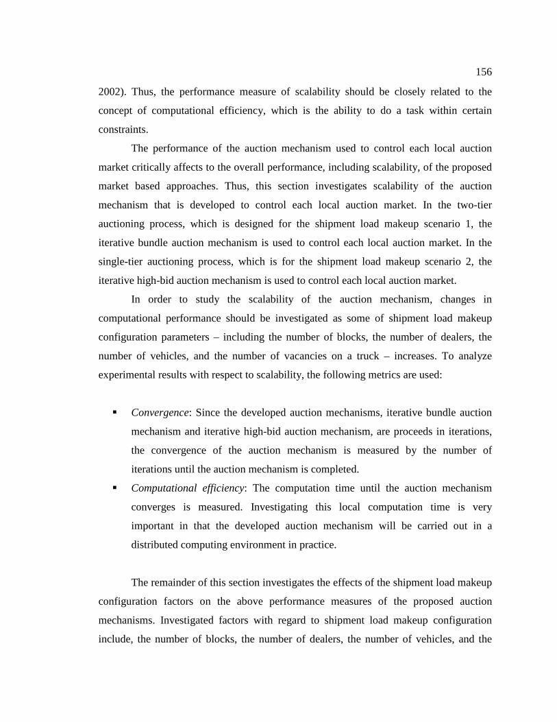
156

2002). Thus, the performance measure of scalability should be closely related to the

concept of computational efficiency, which is the ability to do a task within certain

constraints.

The performance of the auction mechanism used to control each local auction

market critically affects to the overall performance, including scalability, of the proposed

market based approaches. Thus, this section investigates scalability of the auction

mechanism that is developed to control each local auction market. In the two-tier

auctioning process, which is designed for the shipment load makeup scenario 1, the

iterative bundle auction mechanism is used to control each local auction market. In the

single-tier auctioning process, which is for the shipment load makeup scenario 2, the

iterative high-bid auction mechanism is used to control each local auction market.

In order to study the scalability of the auction mechanism, changes in

computational performance should be investigated as some of shipment load makeup

configuration parameters – including the number of blocks, the number of dealers, the

number of vehicles, and the number of vacancies on a truck – increases. To analyze

experimental results with respect to scalability, the following metrics are used:

� Convergence: Since the developed auction mechanisms, iterative bundle auction

mechanism and iterative high-bid auction mechanism, are proceeds in iterations,

the convergence of the auction mechanism is measured by the number of

iterations until the auction mechanism is completed.

� Computational efficiency: The computation time until the auction mechanism

converges is measured. Investigating this local computation time is very

important in that the developed auction mechanism will be carried out in a

distributed computing environment in practice.

The remainder of this section investigates the effects of the shipment load makeup

configuration factors on the above performance measures of the proposed auction

mechanisms. Investigated factors with regard to shipment load makeup configuration

include, the number of blocks, the number of dealers, the number of vehicles, and the

157

number of vacancies on a truck. These fiver factors define the overall size and the

resource availability of a shipment load makeup configuration, and affect the size of the

IP problem and the performance of its solution procedure.

11.3.1 Effect of Number of Blocks

In order to evaluate the effect of the number of blocks on the performance of the

auction mechanism used to control each local auction market, 10 shipment load makeup

instances are generated for each shipment load makeup scenario, where the levels of the

number of blocks are 10, 20, 30, 40, 50, 60, 70, 80, 90, and 100. Each instance has 20

dealers per block and 3 vehicles per dealer, and the other input parameters used for

generating each instance are set to the values shown in Table 11.4. For each of these

shipment load makeup instances, a total of 5 simulation runs are repeated to reduce

random effects.

Table 11.8 and Figure 11.8 summarize the experiment results of testing the effect

of varying the number of blocks on the performance of the local auction mechanism

utilized in the two-tier auctioning process for scenario 1. In Table 11.8, ANo_It denotes

an average number of iterations per local market, L_CompT is an average computation

time per local market, and Acomp_It represents an average computation time per

iteration. As shown in Table 11.8 and Figure 11.8, the effect of the number of blocks is

not significant as far as the number of dealers per block and the number of vehicles per

dealer remains same. This result is very reasonable in that the two-tier auctioning

process, designed in Chapters 9, constructs a local auction market for each block.

158

Table 11.8: Experiment results of testing the effect of varying number of blocks on the performance of the local auction mechanism in two-tier auctioning process (scenario 1).

No_B ANo_D ANo_V TNo_D TNo_V ANo_It computation time

L_CompT Acomp_It

10 20 3 200 600 8.30 0.1263 0.0152

20 20 3 400 1200 8.55 0.1282 0.0149

30 20 3 600 1800 9.33 0.1375 0.0146

40 20 3 800 2400 8.90 0.1331 0.0150

50 20 3 1000 3000 8.88 0.1322 0.0149

60 20 3 1200 3600 9.11 0.1517 0.0167

70 20 3 1400 4200 8.81 0.1422 0.0161

80 20 3 1600 4800 8.78 0.1476 0.0168

90 20 3 1800 5400 8.93 0.1397 0.0156

100 20 3 2000 6000 8.31 0.1195 0.0143

159

Fig. 11.8: Effect of the number of blocks on the performance of the local auction mechanism for scenario 1: (a) average number of iterations, (b) average computation time, and (c) average computation time per iteration.

Table 11.9 and Figure 11.9 summarize the experiment results of investigating the

effect of varying the number of blocks on the performance of the local auction

mechanism used in the single-tier auctioning process for scenario 2. Similar to the local

auction mechanism used in the two-tier auctioning process, the overall performance (e.g.,

convergence and computational efficiency) are not different from each other. However,

as designed in Chapter 10, the number of iterations for the iterative high-bid auction

mechanism is always same as the number of items (e.g. the number of vacancies on a

truck) to be sold in a local market. Finally, the above experimental results clearly show

that the number of blocks does not affect to the performance of the auction mechanism as

far as the number of dealers per block and the number of vehicles per dealer remains

0.04

0.08

0.12

0.16

0.2

10 20 30 40 50 60 70 80 90 100

number of blocks

0.012

0.014

0.016

0.018

0.02

10 20 30 40 50 60 70 80 90 100

number of blocks

6

7

8

9

10

10 20 30 40 50 60 70 80 90 100

number of blocks

(b) average computation time in local market (c) average computation time per iteration

(a) average number of iterations in local market

160

same. This result is very reasonable in that a local auction market is constructed for each

block in the single-tier auctioning process.

Table 11.9: Experiment results of testing the effect of varying number of blocks on the performance of the local auction mechanism in single-tier auctioning process (scenario 2).


L_CompT Acomp_It

10 20 3 200 600 12 0.0729 0.0061

20 20 3 400 1200 12 0.0760 0.0063

30 20 3 600 1800 12 0.0752 0.0060

40 20 3 800 2400 12 0.0720 0.0063

50 20 3 1000 3000 12 0.0753 0.0062

60 20 3 1200 3600 12 0.0741 0.0061

70 20 3 1400 4200 12 0.0734 0.0063

80 20 3 1600 4800 12 0.0736 0.0061

90 20 3 1800 5400 12 0.0735 0.0062

100 20 3 2000 6000 12 0.0742 0.0062

161

Fig. 11.9: Effect of the number of blocks on the performance of the local auction mechanism for scenario 2: (a) average number of iterations, (b) average computation time, and (c) average computation time per iteration.

11.3.2 Effect of Number of Dealers

In order to evaluate the effect of the number of dealers on the performance of the

auction mechanism, 10 shipment load makeup instances are generated for each shipment

load makeup scenario, where the levels of the number of dealers per block are 20, 40, 60,

80, 100, 120, 140, 160, 180, and 200. Each instance has 10 blocks and 3 vehicles per

dealer, and the other input parameters used for generating each instance are given as

shown in Table 11.4. For each of these instances, a total of 5 simulation runs are

repeated.

The experiment results of testing the effect of the number of dealers per block on

the performance of the local auction mechanism for the two-tier auctioning process are

0.06

0.07

0.08

0.09

10 20 30 40 50 60 70 80 90 100

number of blocks

0.005

0.0055

0.006

0.0065

0.007

10 20 30 40 50 60 70 80 90 100

number of blocks


6

8

10

12

14

16

10 20 30 40 50 60 70 80 90 100

number of blocks


162

shown in Table 11.10 and Figure 11.10. As shown in the table and figure, according to

the increase in the number of dealers per block, the convergence speed and computation

time increases linearly, rather than exponentially.

Table 11.10: Experiment results of testing the effect of varying number of dealers on the performance of the local auction mechanism in two-tier auctioning process (scenario 1).


L_CompT Acomp_It

10 20 3 200 600 9.1 0.1339 0.0147

10 40 3 400 1200 9.7 0.2773 0.0285

10 60 3 600 1800 10.7 0.4287 0.0401

10 80 3 800 2400 9.9 0.5531 0.0559

10 100 3 1000 3000 10.2 0.7005 0.0687

10 120 3 1200 3600 10.4 0.8314 0.0799

10 140 3 1400 4200 10.5 0.9811 0.0934

10 160 3 1600 4800 10.7 1.1561 0.1081

10 180 3 1800 5400 10.5 1.1954 0.1237

10 200 3 2000 6000 10.6 1.4258 0.1345

163

Fig. 11.10: Effect of the number of dealers on the performance of the local auction mechanism for scenario 1.

Table 11.11 and Figure 11.11 summarize the experiment results of the effect of

the number of dealers per block on the performance of the local auction mechanism for

the single-tier auctioning process. These results show that the computational complexity

increases linearly, rather than exponentially, as the number of dealers per block increases

for the tested range (20-200).

0

0.05

0.1

0.15

0.2

20 40 60 80 100 120 140 160 180 200

number of blocks per block

0

1

2

3

20 40 60 80 100 120 140 160 180 200

number of dealers per block

6

8

10

12

14

20 40 60 80 100 120 140 160 180 200




164

Table 11.11: Experiment results of testing the effect of varying number of dealers on the performance of the local auction mechanism in single-tier auctioning process (scenario 2).


L_CompT Acomp_It

10 20 3 200 600 12 0.0788 0.0066

10 40 3 400 1200 12 0.1535 0.0128

10 60 3 600 1800 12 0.2317 0.0192

10 80 3 800 2400 12 0.3026 0.0252

10 100 3 1000 3000 12 0.3822 0.0319

10 120 3 1200 3600 12 0.4475 0.0373

10 140 3 1400 4200 12 0.5171 0.0431

10 160 3 1600 4800 12 0.6111 0.0509

10 180 3 1800 5400 12 0.6837 0.0569

10 200 3 2000 6000 12 0.7418 0.0618

165

Fig. 11.11: Effect of the number of dealers on the performance of the local auction mechanism for scenario 2.

11.3.3 Effect of Number of Vehicles

In order to investigate the effect of the number of vehicles on the performance of

the auction mechanism, 8 shipment load makeup instances are generated for each

shipment load makeup scenario. The levels of the number of vehicles per dealer are 1, 2,

3, 4, 5, 6, 7, and 8. Each shipment load makeup instance has 10 blocks and 50 dealers per

block. Thus, the total number of vehicles used in this experimentation is ranging from

500 to 4000. For each of these instances, 5 simulation runs are repeated to decrease

random effects.

6

8

10

12

14

16

20 40 60 80 100 120 140 160 180 200


0

0.25

0.5

0.75

1

20 40 60 80 100 120 140 160 180 200


0

0.025

0.05

0.075

0.1

20 40 60 80 100 120 140 160 180 200




166

Table 11.12 and Figure 11.12 summarize the experiment results of investigating

the effect of varying the number of vehicles per dealer on the performance of the local

auction mechanism used in the two-tier auctioning process for scenario 1. As shown in

the table and figure, according to the increase in the number of vehicles per dealer, the

number of iterations and computation time increases almost linearly.

Table 11.12: Experiment results of testing the effect of varying number of vehicles on the performance of the local auction mechanism in two-tier auctioning process (scenario 1).

No_B ANo_D ANo_V TNo_D TNo_V ANo_It Computation time

L_CompT Acomp_It

10 50 1 500 500 6.2 0.1582 0.0255

10 50 2 500 1000 7.3 0.2498 0.0342

10 50 3 500 1500 9.3 0.3395 0.0365

10 50 4 500 2000 11.5 0.4197 0.0363

10 50 5 500 2500 12.5 0.4717 0.0377

10 50 6 500 3000 13.4 0.5076 0.0379

10 50 7 500 3500 14.9 0.5808 0.0389

10 50 8 500 4000 14.8 0.5819 0.0393

167

Fig. 11.12: Effect of the number of vehicles on the performance of the local auction mechanism for scenario 1.

The effect of the number of vehicles per dealer on the performance of the local

auction mechanism for the single-tier auctioning process is summarized in Table 11.13

and Figure 11.13. These experimental results show that the computational complexity

increases linearly, rather than exponentially, as the number of vehicles per dealer

increases for the tested range (1-8).

0

0.25

0.5

0.75

1

1 2 3 4 5 6 7 8

average number of vehicles per dealer

0

0.015

0.03

0.045

0.06

1 2 3 4 5 6 7 8


0

5

10

15

20

1 2 3 4 5 6 7 8




168

Table 11.13 Experiment results of testing the effect of varying number of vehicles on the performance of the local auction mechanism in single-tier auctioning process (scenario 2).

No_B ANo_D ANo_V TNo_D TNo_V ANo_It Computation time

L_CompT Acomp_It

10 50 1 500 500 12 0.0904 0.0075

10 50 2 500 1000 12 0.1424 0.0118

10 50 3 500 1500 12 0.1938 0.0161

10 50 4 500 2000 12 0.2454 0.0204

10 50 5 500 2500 12 0.2904 0.0242

10 50 6 500 3000 12 0.3460 0.0288

10 50 7 500 3500 12 0.3942 0.0329

10 50 8 500 4000 12 0.3904 0.0325

169

Fig. 11.13 Effect of the number of dealers on the performance of the local auction mechanism for scenario 2.

11.3.4 Effect of Number of Vacancies on a Truck

The effect of the number of vacancies on a tuck on the performance of the auction

mechanism is evaluated by testing 6 shipment load makeup instances, where the levels of

the number of vacancies on a tuck are 8, 10, 12, 14, 16, and 18. Each shipment load

makeup instance has 10 blocks, 50 dealers per block, and 3 vehicles per dealer, and other

input parameters used in this experimentation are set to the values given in Table 11.4.

For each of these instances, a total of 5 simulation runs are repeated.

6

8

10

12

14

16

1 2 3 4 5 6 7 8


0

0.1

0.2

0.3

0.4

0.5

1 2 3 4 5 6 7 8


0

0.01

0.02

0.03

0.04

0.05

10 20 30 40 50 60 70 80




170

As shown in Table 11.14 and Figure 11.14, the effect of the number of vacancies

on a truck is not significant as far as the number of blocks, the number of dealers per

block, and the number of vehicles per dealer remains same.

Table 11.14 Experiment results of testing the effect of varying number of vacancies on a truck on the performance of the local auction mechanism in two-tier auctioning process (scenario 1).

No_B ANo_D ANo_V number of vacancies

ANo_It computation time

L_CompT Acomp_It

10 50 3 8 9.1 0.3307 0.0363

10 50 3 10 9.1 0.0026 0.0365

10 50 3 12 9.3 0.3472 0.0369

10 50 3 14 8.9 0.3322 0.0378

10 50 3 16 9.4 0.3361 0.0358

10 50 3 18 9.3 0.3383 0.0364

171

Fig. 11.14 Effect of the number of vacancies on a truck on the performance of the local auction mechanism for scenario 1.

Table 11.15 and Figure 11.15 summarize the experiment results of testing the

effect of varying the number of vacancies on a truck on the performance of the local

auction mechanism used to control each local market in the single-tier auctioning process

for scenario 2.

Since the iterative high-bid auction mechanism, used for the shipment load

makeup scenario 2, is originally designed to have the fixed number of iterations, which is

the same as the number of vacancies on a truck, it is very clear that the number of

iterations increases linearly as the number of vacancies increases. However, as shown in

Figure 11.15(b), the number of vacancies does not affect the computational efficiency of

0.2

0.25

0.3

0.35

0.4

8 10 12 14 16 18

number of vacancies on a truck

0

0.015

0.03

0.045

0.06

8 10 12 14 16 18


7

8

9

10

11

8 10 12 14 16 18




172

the auction mechanism. Thus, the average computation time per iteration, shown in

Figure 11.15(c), decreases linearly as the number of vacancies on a truck increases.

Table 11.15 Experiment results of testing the effect of varying number of vacancies on a truck on the performance of the local auction mechanism in single-tier auctioning process (scenario 2).

No_B ANo_D ANo_V number of vacancies

ANo_It computation time

L_CompT Acomp_It

10 50 3 8 8 0.1938 0.0242

10 50 3 10 10 0.1942 0.0194

10 50 3 12 12 0.1713 0.0143

10 50 3 14 14 0.1727 0.0123

10 50 3 16 16 0.1907 0.0119

10 50 3 18 18 0.1945 0.0108

173

Fig. 11.15 Effect of the number of vacancies on a truck on the performance of the local auction mechanism for scenario 2.

11.4 Summary of Empirical Analysis

Experimental analysis and validation of the proposed market-based approach is

important part of this study. This chapter presents the experimental analysis results with

experimental setup and generation of a shipment load makeup instance. In order to

conduct experimental analysis, a simulator, which emulates shipment load makeup

processes with the proposed market-based mechanisms, is developed. Using the

simulator, a variety of shipment load makeup instances are thoroughly tested and

analyzed for verifying specific aspects of the market-based mechanism. The experimental

4

8

12

16

20

8 10 12 14 16 18


0

0.1

0.2

0.3

0.4

8 10 12 14 16 18


0

0.01

0.02

0.03

0.04

8 10 12 14 16 18




174

analysis results demonstrate the market-based decentralized approach for shipment load

makeup achieves high level of solution quality and computational efficiency. The results

of the experimental analysis are summarized as follows.

� The two-tier auctioning process, as a market-based approach for the shipment

load makeup scenario 1, provides near optimal solution quality, ranging from

93.2% to 99/9% (average 97.8%) of the optimal solution generated by LINDO,

while the average computation time is about 45.5% of the LINDO solution. As

the number of dealers per block increases, the value of %Eff (computation time in

LINDO / computation time in the market-based approach) decreases.

� The single-tier auctioning process for the shipment load makeup scenario 2 shows

a high level of computational efficiency, 8.23% of the LINDO solution, and

solution quality, ranging 91.8% to 98.4% of the optimal solution. According to

the increase in the number of vehicles, the computation time of the proposed

auctioning process decreases almost exponentially.

� The difference between computational times of the proposed approaches (the two-

tier auctioning process and the single-tier auctioning processes) and a centralized

approach using the IP formulation will become larger when the proposed

auctioning processes are implemented in a multiagent system, where multiple

local auction markets are to be processed simultaneously in distributed local

computers.

� As investigated in Section 11.3, according to the increase in the number of

dealers, the computation time of the both local auction mechanisms (iterative

bundle auction mechanism and iterative high-bid auction mechanism) increase

linearly (see Figures 11.11 and 11.12). A similar result is shown for the effect of

the number of vehicles on the performance of the local auction mechanism (see

Figures 11.13 and 11.14). These results imply that the proposed local auction

mechanisms are scalable and applicable to a practical size of the shipment load

makeup problems and other real-time decision-making problems, because the

computation time per each iteration varies within a second.

175

Chapter 12

Conclusions and Future Research

Dynamics in real-world business operations, such as various unexpected

disruptions and uncertainties, have significant impact on the efficiency of supply chain

management. Recently, as RFID technologies have been widely adopted in various

supply chains environments, visibility of the dynamics in business operations improves,

and allows designing efficient operational models and decision-making strategies.

This thesis is motivated by a real world example relating to outbound logistics of

an automobile manufacturers’ supply chain. In specific, this thesis addresses the shipment

yard operations, such as vehicle deployment and shipment load makeup, where an RFID-

based wireless tracking system provides real-time information of vehicles. The first

consideration is defining the operational specifications and decision-making problems for

current vehicle deployment and shipment load makeup. An understanding of current

operational processes and the RFID technology defines new operational processes for

vehicle deployment and shipment load makeup and corresponding decision-making

models in the RFID-enabled shipment yard. The fundamental change is that decentralized

decision-making model becomes necessary. Multiagent-based information framework

and various market-based control mechanisms deal with these decision-making models in

a decentralized manner and provide adaptable solutions in time. The results of

computational experiments demonstrate that the proposed approaches work effectively in

the given context. The following sections review the major contributions from this

research, identify the managerial implications, and suggest future research.

12.1 Contributions

The major contributions from this research work are as follows:

176

1. This research is among the first to deal with the operational problems in an RFID-

enabled automobile shipment yard, and it identifies the significance and difficulty

of operational problems for vehicle deployment and shipment load makeup. This

study formally specifies these problems by defining the operational performance

measures and constraints of shipment yard operations.

2. This research successfully combines a multiagent-based information architecture,

various auction mechanisms as market-based control approaches, and

mathematical programming models designed by operations research methodology

for the decentralized operational problems in an RFID-enabled shipment yard.

The auction mechanisms facilitated in a multiagent framework effectively support

the distributed and dynamic nature of operational environment and efficiently

process a large amount of distributed information provided from the RFID

system. Furthermore, the proposed multiagent-based information architecture and

market-based control approach allow building an efficient structure for sharing

information collected from the RFID system with multiple supply chain partners,

such as local dealers and transportation resource divisions or 3rd party logistics

providers.

3. This study mathematically formulates the decision-making models for the

shipment yard operations in an RFID-enabled environment. In that management

of a shipment yard is a subsidiary activity of an automobile manufacturer’s

outbound logistics, the mathematical programming model designed in this thesis

successfully integrates the managerial objectives of the shipment yard and other

functional organizations in outbound logistics, such transportation resource

divisions and numerous local dealers.

4. The proposed auction mechanisms, as a market-based control approach, are novel

approaches that effectively incorporate the dynamic, coupled and distributed

177

nature of the shipment yard operational problems. Some of contributions

regarding the auction algorithms proposed in this thesis are:

(i) Two-tier auctioning process (i.e., local auction markets and central auction

market), designed for the shipment load makeup problem, is effective for

decomposing the problem. Distributed local markets determine the set of

potential winning dealer agents and the utility value of the resource, while in

the central auction market the final winning dealer agents are determined by

allocating the resources to block agents which provides maximum revenue

for the resource agent.

(ii) The designed strategic bidding behavior, such as the second-chance bidding

strategy, enhances performance of the auction mechanism by increasing

allocation efficiency.

(iii) The proposed iterative bundle auction mechanism successfully provides an

efficient solution in reasonable time. The winner determination problem in

this auction mechanism is an NP-complete problem. The approximation

algorithm, developed based on the problem structure, enhances

computational performance of the auction mechanism by efficiently solving

the winner determination problem in time.

5. This research investigates the impact of real-time information from the RFID

system on the management of the automobile shipment yard. By designing the

operational decision-making models for the RFID-enabled shipment yard and

solving the models effectively, the value of the RFID system on the shipment

yard’s operations is quantitatively evaluated. The proposed auction mechanisms

under the multiagent computational architecture improve the operational

performance because these auction mechanisms can effectively capture and

respond to the dynamic changes in shipment yard’s operational environment by

utilizing real-time information from the RFID system. Finally the RFID-enabled

information systems, driven by intelligent algorithms, can innovate the

178

performance of supply chain operations with timely information and better

decision-making support.

6. Using the shipment yard operational environment generator, this study tests

various operational scenarios of shipment load makeup and different auction

mechanisms to solve shipment load makeup problems. The experimental analysis

procedure, using various operational scenarios and auction mechanisms, can

provide valuable principles for solution performance analysis models for

shipment load makeup.

12.2 Managerial Implications

One of the most important managerial concerns of the automobile manufacturer is

enhancing the efficiency of shipment yard operations and customer fulfillment by

reducing vehicle dwell time in the shipment yard. Delivering the vehicles to customers

with shorter lead-times can increase the competitiveness and attract potential customers.

Another important goal in managing a shipment yard is to determine the right size buffers

and the right number of yard operators to reduce or eliminate many of the problems that

result in cost overruns and loss of consumption. Excessive operational costs usually arise

when a labor over-supply or under-supply exists (Anderson et al, 1997). Finally,

determining appropriate decisions, under a variety of operational environments, enables

the shipment yard manager to reduce the dwell time of vehicles and increases labor

utilization. In addition, real-time information from the RFID system and advanced

decision-making mechanisms enables achieving enhanced shipment yard operations and

reducing operational costs for the shipment yard, for transportation resource divisions,

and for local dealers. The experimental analysis results clearly show that the RFID-

enabled decision-making system improves the performance of shipment yard operations

as well as accomplishes the objectives of enhancing customer satisfaction and reducing

total labor costs. Specifically, the following observations have meaningful implications:

179

1. Since the shipment yard is not a warehouse for holding inventory, vehicles are not

supposed to stay in the shipment yard longer than expected and should be shipped

within a predefined maximum allowed dwell time. The automobile manufacturer

wishes to reduce the number of vehicles staying in the shipment yard for an

unexpectedly long time. This leads to the reduction of customer waiting time and

then, improves customer satisfaction through meeting order delivery expectations.

Delivering vehicles to customers with shorter lead-times can increase

competitiveness and attract potential customers.

2. The active RFID system reports the location of a vehicle along its movement flow

in real time. This real-time movement information with current location enables

speeding up vehicle deployment and load makeup processes, reducing dwell time

by eliminating unnecessary time delays, and assisting dispatching labor to handle

tasks more efficiently.

3. The operations in the shipment yard can be influenced by exceptions and

disruptions, which the RFID-enabled flexible and adaptable decision-making can

mitigate by quickly sensing and responding to the impact of those events on

operational performance.

4. Under a variety of management circumstances, determining appropriate shipment

yard operations and management parameters enables the shipment yard manager

to optimize operational performance. What-if analysis can be performed by

changing the operational parameters such as the number of block areas, the

number of local dealers, various operational costs, etc.

12.3 Future Research

180

This section describes some possible future research extensions:

1. This research restricts the computational experiment of vehicle deployment to the

case in which an experimental vehicle shipment schedule follows a high-priority-

first-load (HPFL) rule. However the vehicle deployment operation is determined

by considering the shipment load makeup decision made by solving shipment

load makeup problems. To this end, the proposed shipment load makeup model

needs to be integrated into vehicle deployment processes for implementing two

major operational processes in a shipment yard as one integrated form. Effectively

combining these two operational processes to obtain better performance of vehicle

deployment is necessary.

2. The designed shipment load makeup problem, in this research, is restricted to the

case in which a number of local dealers are clustered into a block, based on their

geographical adjacency. In order to generalize the problem, the shipment load

makeup problem can be analyzed without the blocking concept. Consequently, the

problem would then include characteristics of the traveling salesman problem

(TSP). Since TSP is an NP-hard problem, it is necessary to develop more

effective auction mechanisms which can provide adaptable solutions.

3. Traditional auction mechanisms allow price only negotiations where a bid

evaluation is a computationally simple task. However, the need for advanced

auction mechanisms that allow complex bids such as multi-attribute bids has been

raised in many situations (Parkes and Kalagnanam, 2004). Only a small but

steadily growing number of academic papers have considered the multi-attribute

auction. Che (1993) and Branco (1997) provide a thorough analysis of the design

of multi-attribute auction. In an auction of this type, bidders are allowed to submit

multi-attribute bids, and therefore negotiate not just on price but also on quantity

and other qualitative attributes. Typical multi-attribute auctions describe a bid as a

set of attribute value pairs. An approach to handling multiple attributes is to

181

convert qualitative attributes into price equivalents by using a certain set of rules.

Another approach uses decision analysis techniques to assign preferences and

individual value functions to the relevant attributes, and calculate the bid scores

by aggregating attribute value scores (Bichler, 1998; Bichler et al., 1999). These

techniques have their origin in multi-attribute decision analyses (Keeny and

Raiffa, 1993; Bichler and Kalagnanam, 2002). From the understanding of

shipment load makeup decision-making strategies, delivery destination, order

priority, and dwelling time are known as key attributes of a vehicle in a shipment

yard. In that sense, the set of vehicles involved in a dealer agent can be described

by these key attributes and denoted as a multi-dimensional vector. In future

studies, a local auction market for the shipment load makeup can be designed on

the basis of a multi-attribute auction mechanism, and this mechanism can promise

higher market efficiency through more effective information exchange between a

bidder and an auctioneer.

4. Vehicle deployment and shipment load makeup operations are modeled as

periodic or sequential decision-making processes where each decision is not made

independently but made interactively. In other words, a decision made in the

current decision epoch affects later decisions. Therefore, the objective of

shipment yard management is to achieve better long term performance of

operational processes by controlling vehicle deployment and shipment load

makeup decisions in a dynamic environment. In this sense, a Markov decision

process (MDP), widely used for devising optimal control policies in dynamic

planning and sequential decision-making problems (Howard, 1960; Puterman,

1994), would be an effective approach for modeling shipment yard operations and

for capturing the dynamics in an operational environment. Furthermore, an MDP-

based operational model can dynamically build vehicle deployment and shipment

load makeup decision policies using real-time information from the RFID-enabled

system. However a well-known practical limitation exists, such as “curse of

dimensionality.” This implies exponential growth in the time and space required

182

to compute an approximate solution to an MDP problem as the problem

dimension (i.e. state and control spaces) increases (Rust, 1997). To overcome the

“curse of dimensionality,” value function approximation techniques, such as

multi-grid algorithms (Chow and Tsitsiklis, 1991; Rust, 1997), feed-forward

neural networks (Lin and Mitchell, 1992; Bertsekas and Tsitsiklis, 1996), and

gradient descent method (Sutton and Barto, 1998), can be introduced.

5. This thesis has dealt with sharing real-time information, provided from the RFID

system, only for the shipment yard management and part of outbound logistics.

However it could have significant worth for analyzing the value of real-time

information exchange across whole supply chain, including inbound logistics,

manufacturing, outbound logistics, and after-sales. Furthermore, diverse

opportunities exist for leveraging the benefits from real-time information from an

RFID system and intelligent decision-making algorithms, including inventory

control, production scheduling, warehouse management, retailing, etc. The overall

approach in this thesis can be useful as a basis to support such RFID-enabled

decision-making problems.

183

BIBLIOGRAPHY

G. Y. Agbegha, R. H. Ballou, and K. Mathur, “Optimizing auto-carrier loading,”

Transportation Science, 32(2): 174-188, 1998.

B. M. Anderson, K. D. Gremban, and B. A. Young, “Shipyard operational improvement

through process management,” In the National Shipbuilding Research Program:

Annual ship production symposium, 1997.

R. Angeles, “RFID technologies: Supply-chain applications and implementation issues,”

Information System Management, 22(1) 51-65, 2005.

A. Attanasio, A. Fuduli, G. Ghiani, and C. Triki, “Integrated shipment dispatching and

packing problems; a case study,” Journal of Mathematical Modeling and Algorithms,

6(1): 77-85, 2007.

A. Bassamboo, M. Gupta, and S. Juneja, “Efficient winner determination techniques for

internet mult-unit auctions,” In Proceedings of the IFIP Conference on Towards The

E-Society: E-Commerce, E-Business, E-Government, pages 417-430, Zurich,

Switzerland, 2001.

R. Bellman, Dynamic Programming, Princeton University Press, Princeton, NJ, 1957.

J. P. Berg, “A literature survey on planning and control of warehousing systems,” IIE

Transactions, 31(8): 751-762, 1999.

D. P. Bertsekas, “The auction algorithms: a distributed relaxation method for the

assignment problem,” Annals of Operations Research, 14(1): 105-123, 1988.

D. P. Bertsekas, “The auction algorithms for assignment and other network flow

problems: a tutorial,” Interfaces, 20(4): 133-149, 1990.

D. P. Bertsekas, “Auction algorithms for network flow problems: a tutorial introduction,”

Computational Optimization and Applications, 1(1): 7-66, 1992.

184

D. P. Bertsekas and J. N. Tsitsiklis, Neuro-Dynamic Programming, Athena Scientific,

Belmont, Massachusetts, 1996.

M. Bichler, “Decision analysis – a critical enabler for multi-attribute auctions,” In

Proceedings of the 12th Bled Electronic Commerce Conference, Bled, Slovenia, 1998.

M. Bichler, M. Kaukal, and A. Segev, “Multi-attribute auctions for electronic

procurement,” In the First IBM IAC Workshop on Internet Based Negotiation

Technologies, Yorktown Heights, NY, 1999.

M. Bichler and J. Kalagnanam, “Bidding languages and winner determination in multi-

attribute auctions,” Research Report: RC 22478, IBM T. J. Watson Research Center,

Yorktown Heights, NY, 2002.

P. T. Blythe, “RFID for road tolling, road-use pricing and vehicle access control,” In IEE

Colloquium on RFID Technology, pages 8/1-8/16, London, U. K., 1999.

F. Branco, “The design of multidimensional auctions,” RAND Journal of Economics,

28(1): 63-81, 1997.

C. Caplice and Y. Sheffi, “Theory and practice of optimization-based bidding for motor

carriers transport services,” Journal of Business Logistics, 24(2): 109-128, 2003.

M. Caridi and S. Cavalieri, “Multi-agent systems in production planning and control; an

overview,” Production Planning and Control, 15(2): 106-118, 2004.

C. R. Cassady and J. E. Kobza, “A probabilistic approach to evaluate strategies for

selecting a parking place,” Transportation Science, 32(1): 30-42, 1998.

A. Cerino and W. P. Walsh, “Research and application of radio frequency identification

(RFID) technology to enhance aviation security,” In Proceedings of the IEEE National

Aerospace and Electronics Conference (NAECON 2000), pages 127-135, 2000.

Y. K. Che, “Design competition through multidimensional auctions,” RAND Journal of

Economics, 24(4): 668-680, 1993.

185

C. S. Chow and J. N. Tsitsiklis, “An optimal one-way multigrid algorithm for discrete

time stochastic control,” IEEE Transactions on Automatic Control, 36(8): 898-914,

1991.

M. Christiansen, K. Fagerholt, and D. Ronen, “Ship routing and scheduling: status and

perspectives,” Transportation Science, 38(1): 1-18, 2004.

S. H. Clearwater, editor, Market-Based Control - A Paradigm for Distributed Resource

Allocation. World Scientific, Singapore, 1996.

W. Domschke and G. Krispin, “Location and layout planning; a survey,” Operational

Research Spectrum, 19(3): 181-194, 1997.

W. Elmaghraby and P. Keskinocak, “Combinatorial auctions in procurement,” In C.

Billington, T. Harrison, H. Lee, and J. Neale, editors, The Practice of Supply Chain

Management, pages 245-258, Kluwer Academic Publishers, Norwell, MA, 2003.

E. Eskigun, Outbound Supply Chain Network Design for a Large-scale Automotive

Company, Ph.D. Thesis, School of Industrial Engineering, Purdue University, West

Lafayette, IN, 2002.

E. Eskigun, R. Uzsoy, P. V. Preckel, G. Beaujon, S. Krishnan, and J. D. Tew, “Outbound

supply chain network design with mode selection, lead times and capacitated vehicle

distribution centers,” European Journal of Operational Research, 165(1): 182-206,

2005.

M. Fan, J. Stallaert, and A. B. Whinston, “Decentralized mechanism design for supply

chain organizations using an auction market,” Information Systems Research, 14(1): 1-

22, 2003.

K. Finkenzeller, RFID Handbook: Fundamentals and Applications in Contactless Smart

Cards and Identification, 2nd Edition, John Wiley & Sons, Chichester, England, 2003.

M. Florian, J. K. Lenstar, and A. H. G. Rinnooy Kan, “Deterministic production

planning: algorithms and complexity,” Management Science, 26(7): 669-679, 1980.

186

G. M. Gaukler, RFID in Supply Chain Management, Ph.D. Thesis, Department of

Management Science and Engineering, Stanford University, Stanford, CA, 2005.

M. A. Gibney and N. R. Jennings, “Dynamic resource allocation by market-based routing

in telecommunications networks,” In Proceedings of the 2nd International Workshop

on Multi-Agent Systems and Telecommunications, pages 102-117, 1998.

K. R. Gue, “Very high density storage systems,” IIE Transactions, 38(1): 79-90, 2006.

Z. Guo, G. J. Koehler, and A. B. Whinston, “A market-based optimization algorithm for

distributed systems,” Management Science, 53(8): 1345-1358, 2007.

M. A. Hariga and P. L. Jackson, “The warehouse scheduling problem: formulation and

algorithms,” IIE Transactions, 28(2): 115-127, 1996.

F. S. Hiller and G. J. Lieberman, Introduction to Operations Research, 6th Edition,

McGraw-Hill, New York, 1995.

A. Hinkkanen, R. Kalakota, P. Saengcharoenrat, J. Stallaert, and A. B. Whinston,

Distributed Decision Support Systems for Real-time Supply Chain Management Using

Agent Technologies, Readings in Electronic Commerce, Addison-Wesley Longman

Publishing Co., Inc., Boston, MA, 1997.

J. Holler and S. Kumara, “Utilizing radio frequency identification (RFID) in the

healthcare industry,” White Paper, Department of Industrial and Manufacturing

Engineering, The Pennsylvania State University, University Park, PA, 2007.

M. Howard, P. Powell, and R. Vidgen, “Automotive industry information systems: from

mass production to build-to-order,” Journal of Cases on Information Technology, 7:

16-30, 2005.

R. A. Howard, Dynamic Programming and Markov Processes, MIT Press, Cambridge,

1960.

G. Q. Huang, J. S. K. Lau, K. L. Mak, and L. Liang, “Distributed supply-chain project

rescheduling: part I – impacts of information-sharing strategies,” International

Journal of Production Research, 43(24): 5107-5129, 2005.

187

R. Iranpour and D. Tung, “Methodology for optimal design of a parking lot,” Journal of

Transportation Engineering, 115(2): 139-160, 1989.

E. J. Jaselskis, M. R. Anderson, C. T. Jahren, Y. Rodriguez, and S. Njos, “Radio-

frequency identification applications in construction industry,” Journal of

Construction Engineering and Management, 121(2): 189-196, 1995.

M. Jin, S. D. Eksioglu, B. Eksioglu, and H. Wang, “Mode selection for automotive

distribution with quantity discounts,” Networks and Spatial Economics, DOI

10.1007/s11067-007-9020-0, 2007.

P. Jones, C. Clarke-Hill, D. Hiller, and D. Comfort, “The benefits, challenges and

impacts of radio frequency identification technology (RFID) for retailers in the UK,”

Marketing Intelligence & Planning, 23(4): 395-402, 2005.

R. L. Keeny and H. Raiffa, Decision Making with Multiple Objectives: Preferences and

Value Tradeoffs, Cambridge University Press, Cambridge, UK, 1993.

J. Kim, K. Tang, S. Kumara, S. T. Yee, and J. Tew, “Value analysis of location-enabled

radio frequency identification information on delivery chain performance,”

International Journal of Production Economics, In press, 2007.

K. H. Kim and K. T. Park, “A note on a dynamic space-allocation method for outbound

containers,” European Journal of Operational Research, 148(1): 92-101, 2003.

A. Klose and A. Drexl, “Facility location models for distribution system design,”

European Journal of Operational Research, 162(1): 4-29, 2005.

P. Kourouthanassis and G. Roussos, “Developing consumer-friendly pervasive retail

systems,” IEEE Pervasive Computing, 2(2): 32-39, 2003.

N. K. C. Krothapalli and A. V. Deshmukh, “Design of negotiation protocols for multi-

agent manufacturing systems,” International Journal of Production Research, 37(7):

1601-1624, 1999.

188

J. S. K. Lau, G. Q. Huang, K. L. Mak, and L. Liang, “Distributed project scheduling with

information sharing in supply chains: part I – an agent-based negotiation model,”

International Journal of Production Research, 43(22): 4813-4838, 2005.

J. O. Ledyard, M. Olson, D. Porter, J. A. Swanson, and D. P. Torma, “The first use of a

combined value auction for transportation services,” Interfaces, 32(5): 4-12, 2002.

Y. H. Lee and S. Kumara, “Market-based collaborative control of distributed multiple

product development projects,” In N. M. Berry, editor, Proceedings of SPIE, 4208:

73–83, 2000.

Y. H. Lee, Market-based Dynamic Resource Control of Distributed Multiple Projects,

Ph.D. Thesis, Department of Industrial and Manufacturing Engineering, The

Pennsylvania State University, University Park, PA, 2002.

C. Legner and F. Thiesse, “RFID-based facility maintenance at Frankfurt airport,” IEEE

Pervasive Computing, 5(1): 34-39, 2006.

C. J. Li, L. Liu, S. Z. Chen, C. C. Wu, C. H. Huang, and X. M. Chen, “Mobile healthcare

service system using RFID,” In Proceedings of IEEE International Conference on

Networking, Sensing and Control, pages 1014-1019, 2004.

L. J. Lin and T. M. Mitchell, “Memory approaches to reinforcement learning in non-

markovian domains,” Technical Report: CS-92-138, Department of Computer

Science, Carnegie Mellon University, PA, 1992.

D. C. Mattfeld and H. Kopfer, “Terminal operations management in vehicle

transshipment,” Transportation Research Part A, 37(5): 435-452, 2003.

D. C. Mattfeld and H. Orth, “The allocation of storage space for transshipment in vehicle

distribution,” Operational Research Spectrum, 28(4): 681-703, 2006.

R. P. McAfee and J. McMillan, “Auctions and bidding,” Journal of Economic Literature,

25(2): 699-738, 1987.

189

D. McFarlane, S. Sanjay, J. L. Chirn, C. Y. Wong, and K. Ashton, “Auto ID systems and

intelligent manufacturing control,” Engineering Applications of Artificial Intelligence,

16(4): 365-376, 2003.

D. Morley. “Painting trucks at general motors: the effectiveness of a complexity based

approach,” In Embracing Complexity: Exploring the Application of Complex Adaptive

Systems to Business, pages 53- 58, The Ernst and Young Center for Business

Innovation, 1996.

C. Moy, “Better decisions in construction operations,” White Papers in RFID Journal,

2007.

M. L. Ng, K. S. Leong, D. M. Hall, and P. H. Cole, “A small passive UHF RFID tag for

livestock identification,” In Proceedings of IEEE International Symposium on

Microwave, Antenna, Propagation and EMC Technologies for Wireless

Communications (MAPE 2005), pages 67-70, 2005.

E. Nishimura, A. Imai, and S. Papadimitriou, “Berth allocation planning in the public

berth system by genetic algorithms,” European Journal of Operational Research,

131(2): 282-292, 2001.

S. H. Owen and M. S. Daskin, “Strategic facility location: a review,” European Journal

of Operational Research, 111(3): 423-447, 1998.

D. C. Parkes, “iBundle: an efficient ascending price bundle auction,” In Proceedings of

the 1st ACM Conference on Electronic Commerce (EC-99), pages 148-157, 1999.

D. C. Parkes and L. H. Ungar, “Iterative combinatorial auctions: theory and practice,” In

Proceedings of the 17th National Conference on Artificial Intelligence (AAAI-00),

pages 74-81, Austin, TX, 2000.

D. C. Parkes, Iterative Combinatorial Auctions: Achieving Economic and Computational

Efficiency, Ph.D. Thesis, Department of Computer and Information Science,

University of Pennsylvania, Philadelphia, PA, 2002.

D. C. Parkes and J. Kalagnanam, “Iterative multiattribute Vickrey auctions,”

Management Science Special Issue on Electronic Markets, 2004.

190

W. B. Powell, B. Bouzaiene-Ayari, and H. P. Simao, “Dynamic models for freight

transportation,” Handbooks in Operations Research and Management Science:

Transportation, G. Laporte and C. Barnhart, editors, Elsevier, Amsterdam, 2007.

K. Prouskas, A. Patel, J. Pitt, and J. Barria, “A multi-agent system for intelligent network

load control using a market-based approach,” In Proceedings of the 4th International

Conference on Multi-Agent Systems, pages 231-238, 2000.

M. L. Puterman, Markov Decision Processes, John Wiley & Sons, New York, 1994.

J. Rust, “Using randomization to break the curse of dimensionality,” Econometrica,

65(3): 487-516, 1997.

Y. Sakurai, M. Yokoo, and K. Kamei, “An efficient approximate algorithm for winner

determination in combinatorial auctions,” In Proceedings of the 2nd ACM Conference

on Electronic Commerce (EC-00), pages 30-37, Minneapolis, MN, 2000.

J. A. Sauter, H. V. D. Parunak, and J. Goic, “ANTS in the supply chain,” In Workshop on

Agent for Electronic Commerce at Agents, Seattle, WA, 1999.

M. Savelsberg, and M. Sol, “The general pickup and delivery problem,” Transportation

Science, 29(1): 17-19, 1995.

C. Saygin, “Adaptive inventory management using RFID data,” International Journal of

Advanced Manufacturing Technology, 32: 1045-1051, 2007.

Y. Sheffi, “Combinatorial auctions in the procurement of transportation service,”

Interfaces, 34(4): 245-252, 2004.

W. Shen and D. H. Norrie, “Agent-based systems for intelligent manufacturing: state-of-

the-art survey,” International Journal of Knowledge and Information Systems, 1(2):

129-156, 1999.

R. Sikora and M. J. Shaw, “Coordination mechanisms for multi-agent manufacturing

systems: application to integrated manufacturing scheduling,” IEEE Transactions on

Engineering Management, 44(2): 175-187, 1997.

191

K. Srinivasan, S. Kekre, and T. Mukhopadhyay, “Impact of electronic data interchange

technology on JIT shipments,” Management Science, 40(10): 1291-1304, 1994.

G. Steiner, “On the complexity of dynamic programming for sequencing problems with

precedence constraints,” Annals of Operations Research, 26(1): 103-123, 1990.

R. S. Sutton and A. G. Barto, Reinforcement Learning: An Introduction, MIT Press,

Cambridge, MA, 1998.

K. P. Sycara, S. F. Roth, N. Sadeh, and M. S. Fox “Resource allocation in distributed

factory scheduling,” IEEE Expert, 6(1): 29-40, 1991.

R. Tadei, G. Perboli, and F. D. Croce, “A heuristic algorithm for the auto-carrier

transportation problem,” Transportation Science, 36(1): 55-62, 2002.

K. Tang, S. Kumara, S. T. Yee, and J. Tew, “Wireless-based dynamic optimization for

load makeup using auction mechanism,” In Proceedings of Industrial Engineering

Research Conference (IERC), on CD, 2004.

D. J. Thomas and P. M Griffin, “Coordinated supply chain management,” European

Journal of Operational Research, 94(1): 1-15, 1996.

A. Trevarthen, “The national livestock identification system: the importance of

traceability in E-business,” Journal of Theoretical and Applied Electronic Commerce

Research, 2(1): 49-62, 2007.

O. Ulgen and S. S. Upendram, “Productivity simulation in the automotive industry,” In

M. Ades and R. Fray, editors, Proceedings of Simulators International XIV

(Simulation Multi-conference), pages 199-204, 1997.

I. F. A. Vis and R. Koster, “Transshipment of containers at a container terminal: an

overview,” European Journal of Operational Research, 147(1): 1-16, 2003.

C. A. Waldspurger, T. Hogg, B. A. Huberman, J. O. Kephart, and W. S. Stornetta,

“Spawn: a distributed computational economy,” IEEE Transactions on Software

Engineering, 18(2): 103-117, 1992.

192

W. E. Walsh and M. P. Wellman, “A market protocol for decentralized task allocation,”

In Proceedings of the Third International Conference on Multi-Agent Systems, pages

325–332, Seattle, WA, 1998.

W. E. Walsh, M. P. Wellman, P. R. Wurman, and J. K. MacKie-Mason, “Some

economics of market-based distributed scheduling,” In Proceedings of the 18th

International Conference on Distributed Computing Systems, pages 612–621,

Amsterdam, The Netherlands, 1998.

S. W. Wang, W. H. Chen, C. S. Ong, L. Liu, and Y. W. Chuang, “RFID application in

hospitals: a case study on a demonstration RFID project in a Taiwan hospital,” In

Proceedings of the 39th Annual Hawaii International Conference on System Sciences,

pages 184-193, 2006.

L. A. Wolsey and G. L. Nemhauser, Integer and Combinatorial Optimization, John

Wiley & Sons, Inc., New York, 1999.

T. Wu, N. Ye, and D. Zhang, “Comparison of distributed methods for resource

allocation,” International Journal of Production Research, 43(3): 515-536, 2005.

S. T. Yee, J. Tew, K. Tang, J. Kim, and S. Kumara, “Radio frequency identification

(RFID)-enabled dynamic optimization innovates vehicle delivery of General Motors,”

submitted to International Journal of Production Economics, 2007.

VITA

Jindae Kim

Jindae Kim was born in Korea in 1973. He received his B.S. and M.S. degrees in

Industrial Engineering from Inha University in 1999 and 2001 respectively. During his

B.S. and M.S. study his major research interest was in the area of computer aided

manufacturing and distributed manufacturing systems. In 2001 fall, he enrolled in the

Ph.D. program in Industrial Engineering at the Pennsylvania State University. During his

Ph.D. study he was employed as a research assistant or a teaching assistant in the

department of Industrial Engineering. As a research assistant, he participated in three

major research projects: (1) “Vehicle Deployment and Load Makeup system (DLMS) in

Wireless Environment” funded by General Motors Research and Development Center,

(2) “Integrated Diagnostics into Ground Equipment Study” funded by United States

Marine Corp., and (3) “Enabling Logistics with Portable and Wireless Technology

Study” funded by United States Marine Corp., under supervision of Dr. Soundar Kumara.

His current research interests include decentralized dynamic control using market-based

mechanisms, multiagent-based information systems, and dynamic control for RFID-

enabled computational models, all in the context of supply chain and logistics,

communication and sensor networks, and service engineering. He is a member of

Institute of Industrial Engineers (IIE) and Institute for Operations Research and

Management Sciences (INFORMS).

IN RFID- E

Documents

Transcript of IN RFID- E