IMPROVING TIME SERIES PREDICTION USING RECURRENT NEURAL NETWORKS

THESIS FOR THE DEGREE OFMASTER OFSCIENCE

IMPROVING TIME SERIES PREDICTION

USING RECURRENTNEURAL NETWORKS

AND EVOLUTIONARY ALGORITHMS

ERIK HULTHEN

Division of MechatronicsDepartment of Machine and Vehicle Systems

CHALMERS UNIVERSITY OF TECHNOLOGYGoteborg, Sweden, 2004

Improving Time Series Prediction using RecurrentNeural Networks and Evolutionary AlgorithmsERIK HULTHEN

c© ERIK HULTHEN, 2004

Division of MechatronicsDepartment of Machine and Vehicle SystemsChalmers University of TechnologySE-412 96 GoteborgSwedenTelephone: +46 (0)31–772 1000

Chalmers ReproserviceGoteborg, Sweden, 2004

Improving Time Series Predictionusing Recurrent Neural Networksand Evolutionary AlgorithmsERIK HULTHENDivision of MechatronicsDepartment of Machine and Vehicle SystemsChalmers University of Technology

Abstract

In this thesis, artificial neural networks (ANNs) are used for prediction of financial andmacroeconomic time series. ANNs build internal models of the problem and are there-fore suited for fields in which accurate mathematical modelscannot be formed, e.g.meteorology and economics. Feedforward neural networks (FFNNs), often trainedwith backpropagation, constitute a common type of ANNs. However, FFNNs sufferfrom lack of short-term memory, i.e. they respond with the same output for a giveninput, regardless of earlier inputs. In addition, backpropagation only tunes the weightsof the networks and does not generate an optimal design. In this thesis, recurrentneural networks (RNNs), trained with an evolutionary algorithm (EA) have been usedinstead. RNNs can have short-term memory and the EA has the advantage that it af-fects the architecture of the networks and not only the weights. However, the RNNsare often hard to train, i.e. the training algorithm tends toget stuck in local optima.In order to overcome this problem, a method is presented in which the initial popu-lation in the EA is an FFNN, pre-trained with backpropagation. During the evolutionfeedback connections are allowed, which will transform theFFNN to an RNN.

The RNNs obtained with both methods outperform both a predictor and the FFNNtrained with backpropagation on several financial and macroeconomic time series. Theimprovement of the prediction error is small, but significant (a few per cent for thevalidation data set).

Key words: time series prediction, evolutionary algorithms, recurrent neural networks

i

Acknowledgements

I would like to thank my supervisor Dr. Mattias Wahde for his inspiration, support, andtempo. I am also grateful to Jimmy Pettersson for all his helpthroughout the course ofthis work.

Erik HulthenGoteborg, January, 2004

iii

Table of Contents

1 Introduction 1

1.1 Motivation . . . . . . . . . . . . . . . . . . . . . . . . . . . . . . . . 1

1.2 Related work . . . . . . . . . . . . . . . . . . . . . . . . . . . . . . 2

1.3 Objectives . . . . . . . . . . . . . . . . . . . . . . . . . . . . . . . . 3

2 Methods 5

2.1 Artificial neural networks . . . . . . . . . . . . . . . . . . . . . . . . 5

2.1.1 Feedforward neural networks . . . . . . . . . . . . . . . . . 6

2.1.2 Recurrent Neural Networks . . . . . . . . . . . . . . . . . . 7

2.2 Training algorithms . . . . . . . . . . . . . . . . . . . . . . . . . . . 10

2.2.1 Backpropagation . . . . . . . . . . . . . . . . . . . . . . . . 10

2.2.2 Evolutionary algorithms . . . . . . . . . . . . . . . . . . . . 12

3 Time series prediction 17

3.1 Introduction . . . . . . . . . . . . . . . . . . . . . . . . . . . . . . . 17

3.1.1 Difference series . . . . . . . . . . . . . . . . . . . . . . . . 17

3.1.2 Scaling . . . . . . . . . . . . . . . . . . . . . . . . . . . . . 18

3.2 Benchmarks . . . . . . . . . . . . . . . . . . . . . . . . . . . . . . 19

3.2.1 Naive strategy . . . . . . . . . . . . . . . . . . . . . . . . . . 19

3.2.2 Exponential Smoothing . . . . . . . . . . . . . . . . . . . . . 19

3.3 FFNNs trained with BP . . . . . . . . . . . . . . . . . . . . . . . . 19

3.4 RNNs trained with GA . . . . . . . . . . . . . . . . . . . . . . . . . 21

3.4.1 Fitness . . . . . . . . . . . . . . . . . . . . . . . . . . . . . 22

3.5 RNNs generated from FFNNs . . . . . . . . . . . . . . . . . . . . . 22

v

vi TABLE OF CONTENTS

4 Results 23

4.1 Introduction . . . . . . . . . . . . . . . . . . . . . . . . . . . . . . . 23

4.2 Time series . . . . . . . . . . . . . . . . . . . . . . . . . . . . . . . 23

4.2.1 USD-JPY exchange rate . . . . . . . . . . . . . . . . . . . . 23

4.2.2 US unemployment rate . . . . . . . . . . . . . . . . . . . . . 24

4.2.3 Dow Jones Industrial Average . . . . . . . . . . . . . . . . . 25

4.3 Conclusion . . . . . . . . . . . . . . . . . . . . . . . . . . . . . . . 26

APPENDED PAPER

Appended paper

This thesis contains the paper listed below. References to the paper will be made usingthe Roman numeral associated with the paper.

I. Erik Hulthen and Mattias Wahde, Improved time series prediction using evo-lutionary algorithms for the generation of feedback connections in neural net-works, accepted for publication inProceedings of Computational Finance 2004,Bologna, Italy, April 2004.

vii

Chapter 1

Introduction

In this thesis recurrent neural networks, trained with evolutionary algorithms, are usedfor time series prediction. The results of the predictions are compared with results fromfeedforward neural networks, trained with backpropagation, and also with some othermethods commonly used for time series prediction. This chapter introduces the subjectand motivates the approach used in this thesis. Chapters 2 and 3 describe the methodsused and time series prediction, respectively. In chapter 4the results are reported anddiscussed.

1.1 Motivation

In time series prediction the task is to forecast the next value (values) in a data set.There are several fields in which time series prediction is ofcentral importance, e.g.meteorology, geology, finance, and macroeconomics. Typically in those fields, thereexists no accurate models of the system, and therefore the series are studied from aphenomenological, model-free point of view. In the physical sciences, where modelsare common, the use of model-free time series prediction is less common. Artificialneural networks (ANNs) are often used for time series prediction because of their abil-ity to build their own internal models. A common method is to train feedforward neuralnetworks (FFNNs) with backpropagation [5]. The method is easy to use and generallyarrives quickly at small prediction errors. However, thereare some drawbacks of us-ing this method. First, in the training of an FFNN, by whatever method, one can neverovercome the lack of short-term memory, illustrated in Fig.1.1, and an FFNN is thusdependent on the number of lookback steps (further described in section 3.3). Second,backpropagation only tunes the weights in the FFNN and does not affect the designof the network. In order to achieve short-term memory a recurrent neural network(RNN), i.e. an ANN with feedback connections, can be used. AnRNN can, in princi-ple, store all former input signals and is thus not dependenton the number of lookback

1

2 CHAPTER 1. INTRODUCTION

Fig. 1.1: An FFNN will always produce the same output for a given input.

steps. However, these networks cannot be trained with standard backpropagation. Inthis thesis evolutionary algorithms (EA) are used instead.Using an EA may also pro-vide the advantage that the design of the networks becomes non-static, i.e. during thetraining not only the weights can be subject to change but also the architecture of theconnections between the neurons and the size of the network.

Here a new method is presented, in which an FFNN is first trained with back-propagation, and then evolved further with an EA. The FFNN, duplicated and slightlymutated, forms the initial population of the EA. During the evolution feedback con-nections are allowed, i.e. the FFNN becomes an RNN if needed.

In order to illustrate the limitations of FFNNs a synthetic time series was generated,containing two situations with the same input values but different desired outputs, asshown in Fig. 1.1. The number of lookback steps was equal to 3 and the remaining33 values were used for training and testing. The RMS distances between the realdata set and the predictions were 0.0139, 0.0120, and 0.0080for the FFNN, the RNNtrained with random initial population, and the RNN trainedwith the FFNN as initialpopulation, respectively. These results clearly illustrate the drawbacks caused by thelack of short-term memory in FFNNs.

1.2 Related work

ANNs have been used for time series prediction by several authors, e.g. [4], [3], and[7]. Many time series of interest, e.g. financial time series, have a high level of noisewhich is not always a result of insufficient measurements (which are often exact in thecase of financial data) but the fact that the series come from systems with many diffuseinfluences, e.g. human psychology in financial series. On theother hand filtering thesignal too much will take away small signs in the series that can give a hunch of thecoming turns. In [4], the use of an RNN is preceded by preprocessing (differencingand log compression) and translation to a symbolic encodingwith a self-organizing

1.3. OBJECTIVES 3

map. The output from the RNN is used to build a deterministic finite state automatondescribing some trend mechanisms. This procedure led to lower noise levels. FFNNswere used with success in [3] for prediction of USD-EUR exchange rate. The resultswere compared with other forecasting techniques using several comparison methods.In [7] the US Index of Industrial Production was forecast with an ANN that gavesuperior results compared to traditional methods.

Backpropagation has been used for training ANN in many situations, see e.g. [5].Using an EA for evolving ANNs has been proposed by e.g. Yao [13]. Other ways toobtain ANNs with short-term memory is backpropagation through time (BPTT), de-scribed in [10]. In these networks each neuron has a connection to all neurons, N timesteps back. However, the design of the network is still static and has to be specifiedbeforehand, and one of the motivations for using ANNs is justits structural flexibilitywhich is thus lost if BPTT is used. Another gradient-based method for training ANNsis real-time recurrent learning [11], but this method has the same drawbacks as BPTT.

1.3 Objectives

The objectives for this thesis are

• to investigate whether it is possible to obtain better time series prediction us-ing RNNs trained with evolutionary algorithms instead of FFNNs trained withbackpropagation.

• to test if an FFNN, trained with backpropagation, can be usedsuccessfully andefficiently to form an initial population in an EA that evolves RNNs for timeseries prediction.

Chapter 2

Methods

This chapter will introduce ANNs and their training algorithms, respectively. The timeseries used for prediction are transformed to data sets withinput-output signals, andwill be described in detail in chapter 3.

2.1 Artificial neural networks

ANNs are clusters of simple, non-linear function units called neurons, and are stronglyinspired by biological neural networks found in animal brains. The history of artifi-cial neural networks (ANNs) goes back to 1943 when McCullochand Pitts presenteda formula for artificial neurons that is basically the same asis used today [5]. Theneurons are connected to each other via connections that transfer information. Theconnections, also called synapses, weigh the transferred signals. A neuron, shown inFig. 2.1, consists of a summarizer and an activation function. The summarizer forms asum of the input signals and a bias term, and gives the result to the activation function,which is the non-linear part of the neuron. One of its functions is to limit the output ofthe neuron to a given range, often [-1,1] or [0,1]. The outputof the activation functionis the output of the neuron itself.

Applications for ANNs can be found in various fields, e.g. thenatural sciences,technology, and economics. A common application is image recognition, e.g. facerecognition, automatic zip code reading, and analysis of satellite images [9]. ANNscan also be used as artificial brains in autonomous robots [8]. Another field in whichANNs are used is non-linear control. Time series predictionis also an important field,and constitutes the application in this thesis (described more in chapter 3).

There are two main reasons for the large computing power of ANNs [5]. First,their parallel distributed structure, which allows the networks to break down complexcomputation tasks into several easier ones, and second, thepossibility to learn andmake generalizations. The generalization makes it possible for an ANN to deliver a

5

6 CHAPTER 2. METHODS

Bias

Σ

Fig. 2.1: The architecture of an artificial neuron: input signals, a bias term, a summa-rizer, an activation function, and an output signal.

reasonable output even if the given inputs were not part of the training set. This is alsothe reason for the robustness, i.e. insensitivity to noise,of ANNs. As an example, inface recognition, the image presented to the ANN as input is rarely exactly the sameevery time, but a well-trained ANN may still be able to give the right output. Anotherbenefit of using ANNs is that they are model-free, i.e. it is not necessary to have amathematical model of the system producing the inputs and outputs. This is especiallyimportant in application where the systems behind the data set are often difficult tomodel.

Here, a description of the two kinds of networks that have been used in this thesiswill follow.

2.1.1 Feedforward neural networks

The feedforward neural networks, FFNNs, used here consist of input units and twolayers of neurons as shown in Fig. 2.2. The number of input units and the number ofneurons are constant for each data set. In this thesis, the number of output neurons isalways equal to one. Each neuron has a connection to every neuron or input unit in theprevious layer.

Neurons

Each neuron consists of a summarizer and an activation function. The summarizercollects the signals from earlier layers and adds a biasbi. The activation function,σ,in all neurons is given by

σ (s) = tanh (βs) (2.1)

2.1. ARTIFICIAL NEURAL NETWORKS 7

Input layer Hidden layer Output layer

Fig. 2.2: A feedforward neural network. The circles are neurons, the boxes are inputunits, and the arrows are connection weights.

whereβ is a constant. Thus, the outputs from the neurons are computed as

yi = σ

(

nx∑

j=1

wijxj + bi

)

, i = 1, . . . , n, (2.2)

wherenx is the number of neurons or input units in the previous layer,xj are the signalsfrom that layer, andwij are the corresponding connections between the previous layerand the current layer. The bias term of neuroni, bi, is used by the neuron to generatean output signal in the absence of input signals.

2.1.2 Recurrent Neural Networks

In contrast to FFNNs, RNNs may have connections (synapses) to all neurons in thenetwork, i.e. there exists no neuron layers. This brings thefact that there is no obviousorder for computing the output of the neurons. In biologicalneural networks, theproblem with computing order does not exist. Instead, a biological neural network isa distributed processor allowing all neurons to execute independently. Because of itsnon-layered structure an RNN is more nature-like than an FFNN. In addition, RNNshave the possibility to maintain signals even after the input signals have disappeared.Thus, properly constructed RNNs have a short-term memory (see below).


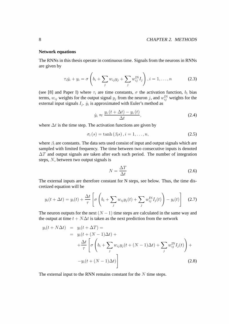
Network equations

The RNNs in this thesis operate in continuous time. Signals from the neurons in RNNsare given by

τiyi + yi = σ

(

bi +∑

j

wijyj +∑

j

wINij Ij

)

, i = 1, . . . , n (2.3)

(see [8] and Paper I) whereτi are time constants,σ the activation function,bi biasterms,wij weights for the output signalyj from the neuronj, andwIN

ij weights for theexternal input signalsIj. yi is approximated with Euler’s method as

yi ≈yi (t + ∆t) − yi (t)

∆t, (2.4)

where∆t is the time step. The activation functions are given by

σi (s) = tanh (βis) , i = 1, . . . , n, (2.5)

whereβi are constants. The data sets used consist of input and outputsignals which aresampled with limited frequency. The time between two consecutive inputs is denoted∆T and output signals are taken after each such period. The number of integrationsteps,N , between two output signals is

N =∆T

∆t(2.6)

The external inputs are therefore constant for N steps, see below. Thus, the time dis-cretized equation will be

yi(t + ∆t) = yi(t) +∆t

τ

[

σ

(

bi +∑

j

wijyj(t) +∑

j

wINij Ij(t)

)

− yi(t)

]

(2.7)

The neuron outputs for the next(N − 1) time steps are calculated in the same way andthe output at timet + N∆t is taken as the next prediction from the network

yi(t + N∆t) = yi(t + ∆T ) =

= yi(t + (N − 1)∆t) +

+∆t

τ

[

σ

(

bi +∑

j

wijyj(t + (N − 1)∆t) +∑

j

wINij Ij(t)

)

+

−yi(t + (N − 1)∆t)

]

(2.8)

The external input to the RNN remains constant for theN time steps.

2.1. ARTIFICIAL NEURAL NETWORKS 9

t

t

∆T

∆T

∆T + ∆t

∆T + ∆t

2∆T

2∆T

3∆T

3∆T

Input signals

Neuron signals

2∆T + ∆t

2∆T + ∆t

3∆T + ∆t

3∆T + ∆t

Fig. 2.3: Dynamical properties of an RNN.

Dynamical properties

As mentioned above, the RNNs used here operate in continuoustime. Data points are,however, provided at discrete time steps. The external input to the RNN only changeswhen a new data point arrives. However, in the time period (oflength∆T ) betweentwo data points, the internal dynamics of the RNN unfolds according to Eq. 2.8. Anexample is shown in Fig. 2.3.

Note that an FFNN, as specified in section 2.1.1, is a special case of an RNN,namely one lacking feedback connections, and with all time constantsτi approachingzero. In principle, neurons may be affected by earlier inputsignals (depending on timeconstraints). Thus, an RNN may contain a memory which is an advantage comparedto the FFNN whose output is only affected by the current inputsignals.

Network elements

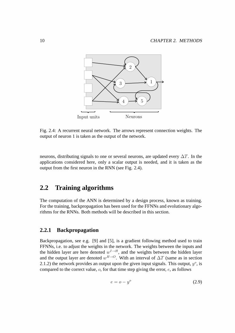
The RNNs consist of neurons and input units. As shown in Fig. 2.4, the connectionweights may connect neurons both to input elements and neurons (note that autocon-nections are allowed). The number of connections from an input unit or a neuron isset individually between zero and a maximum,Mc. An unconnected neuron has, ofcourse, no effect on the output of the network.

The input units, which act as intermediaries between the input signals and the


Input units Neurons

1

2

3

4 5

Fig. 2.4: A recurrent neural network. The arrows represent connection weights. Theoutput of neuron 1 is taken as the output of the network.

neurons, distributing signals to one or several neurons, are updated every∆T . In theapplications considered here, only a scalar output is needed, and it is taken as theoutput from the first neuron in the RNN (see Fig. 2.4).

2.2 Training algorithms

The computation of the ANN is determined by a design process,known as training.For the training, backpropagation has been used for the FFNNs and evolutionary algo-rithms for the RNNs. Both methods will be described in this section.

2.2.1 Backpropagation

Backpropagation, see e.g. [9] and [5], is a gradient following method used to trainFFNNs, i.e. to adjust the weights in the network. The weightsbetween the inputs andthe hidden layer are here denotedwI→H, and the weights between the hidden layerand the output layer are denotedwH→O. With an interval of∆T (same as in section2.1.2) the network provides an output upon the given input signals. This output,yo, iscompared to the correct value,o, for that time step giving the error,e, as follows

e = o − yo (2.9)

2.2. TRAINING ALGORITHMS 11

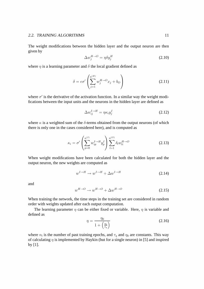
The weight modifications between the hidden layer and the output neuron are thengiven by

∆wH→Oj = ηδyH

j (2.10)

whereη is a learning parameter andδ the local gradient defined as

δ = eσ′

n(H)∑

j=1

wH→Oj xj + bO

(2.11)

whereσ′ is the derivative of the activation function. In a similar way the weight modi-fications between the input units and the neurons in the hidden layer are defined as

∆wI→Hij = ηκiy

Ij (2.12)

whereκ is a weighted sum of theδ-terms obtained from the output neurons (of whichthere is only one in the cases considered here), and is computed as

κi = σ′

n(I)∑

p=0

wI→Hip yI

p

n(O)∑

l=1

δlwH→Oli (2.13)

When weight modifications have been calculated for both the hidden layer and theoutput neuron, the new weights are computed as

wI→H → wI→H + ∆wI→H (2.14)

and

wH→O → wH→O + ∆wH→O (2.15)

When training the network, the time steps in the training setare considered in randomorder with weights updated after each output computation.

The learning parameterη can be either fixed or variable. Here,η is variable anddefined as

η =η0

1 +(

nl

τη

) (2.16)

wherenl is the number of past training epochs, andτη andη0 are constants. This wayof calculatingη is implemented by Haykin (but for a single neuron) in [5] and inspiredby [1].


Selection

Initialize population

Decoding and evaluation

Mutation

Continue?

No

Yes

Mutate ∆t

Structural mutation

50% 50%

Full mutation Creep mutation

Fig. 2.5: Schematic representation of the implemented GA.

2.2.2 Evolutionary algorithms

Evolutionary algorithms is a general term for training methods inspired by darwinianevolution, and includes e.g. genetic algorithms (GA), genetic programming (GP), andEvolution strategies (ES) [9]. The methods have been used inmany different applica-tions e.g. optimization, construction of neural networks,time series prediction, controlsystem identification, reverse engineering, and autonomous robot control. As the nameimplies, these methods are strongly inspired by natural evolution. Just as in nature,species form populations consisting of individuals. In nature individuals are livingbeings but in EAs the individuals are potential solutions tothe problem under consid-eration. The variables of the problem are coded in the genomes of the individuals. Agenome may consist of one or several chromosomes, which in turn consist of stringsof values, known as genes. The solutions are tested and the individuals are given ameasure of goodness, referred to as the fitness value. The higher the fitness, the largerthe chance for an individual to be selected as parent to new individuals in the next gen-eration. Reproduction may be sexual or asexual and mutations may occur. Althoughthe process of an EA contains stochastic parts it should be stated clearly that evolutionis not a random search. For a deeper review of this subject, [2] is recommended.

The EA used here is a modified genetic algorithm (GA). The maindifferences com-pared to a standard GA are that there is no crossover, structural mutations are added,and the mutation rate varies with the size of the network encoded in the chromosome(see Eq. 2.24 below). The crossover operator, which combines genes from two indi-viduals, is rarely useful when evolving neural networks andis therefore not used here.In this thesis the genomes always consist of only one chromosome, but the number of


Number of neuronsTime step

Input unit 1Input unit 2

Neuron 1Neuron 2

Neuron 3

τβb

Connection 1Connection 2

On/OffNeuronWeight

Fig. 2.6: The description of the RNN is encoded in a chromosome.

genes in a chromosome, and thus the number of neurons in the corresponding RNNs,may vary. The general progress of the GA used here can been seen in Fig. 2.5. TheRNNs are then created from the decoded parameters of the chromosomes and tested intheir application (in this case time series prediction). The test will give a fitness valueback to the GA which is used for selection of parents used in the formation of the newgeneration. The selection method used here is tournament selection, described laterin this section. The new generation is created asexually, meaning that the individu-als (before mutation) are copies of their parents. The new generation is then exposedto mutations which will distinguish the genomes of the offsprings from those of theirparents. When the new generation has been created a new evaluation takes place. Themutation is, as shown in Fig. 2.5, made in several steps. The structural mutations areessential since they let the RNN change size to adapt to the problem at hand. Themutation procedure will be described in detail below.

Encoding

The encoding of the chromosomes can be seen in Fig. 2.6. The chromosomes consistof genes represented by real numbers in the range[−1, 1]. The number of neurons,n,in the RNN is given by

n = |G1|Mn (2.17)

whereG1 is the first gene in the chromosomeG andMn is the maximum number ofneurons permitted.Mn is constant during the entire training. The time step∆t (as in


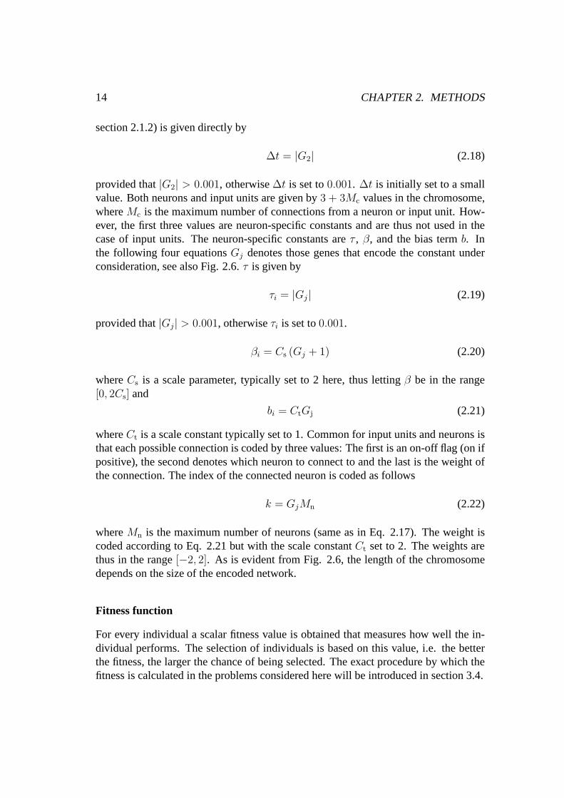
section 2.1.2) is given directly by

∆t = |G2| (2.18)

provided that|G2| > 0.001, otherwise∆t is set to0.001. ∆t is initially set to a smallvalue. Both neurons and input units are given by3 + 3Mc values in the chromosome,whereMc is the maximum number of connections from a neuron or input unit. How-ever, the first three values are neuron-specific constants and are thus not used in thecase of input units. The neuron-specific constants areτ , β, and the bias termb. Inthe following four equationsGj denotes those genes that encode the constant underconsideration, see also Fig. 2.6.τ is given by

τi = |Gj | (2.19)

provided that|Gj| > 0.001, otherwiseτi is set to0.001.

βi = Cs (Gj + 1) (2.20)

whereCs is a scale parameter, typically set to 2 here, thus lettingβ be in the range[0, 2Cs] and

bi = CtGj (2.21)

whereCt is a scale constant typically set to 1. Common for input unitsand neurons isthat each possible connection is coded by three values: The first is an on-off flag (on ifpositive), the second denotes which neuron to connect to andthe last is the weight ofthe connection. The index of the connected neuron is coded asfollows

k = GjMn (2.22)

whereMn is the maximum number of neurons (same as in Eq. 2.17). The weight iscoded according to Eq. 2.21 but with the scale constantCt set to 2. The weights arethus in the range[−2, 2]. As is evident from Fig. 2.6, the length of the chromosomedepends on the size of the encoded network.

Fitness function

For every individual a scalar fitness value is obtained that measures how well the in-dividual performs. The selection of individuals is based onthis value, i.e. the betterthe fitness, the larger the chance of being selected. The exact procedure by which thefitness is calculated in the problems considered here will beintroduced in section 3.4.


Fig. 2.7: Two types of structural mutations are used. In the top panel a neuron isremoved. In the bottom panel a new neuron is added gently (i.e. using weak connectionweights).

Tournament Selection

Tournament selection, used for selecting parents when forming new generations, oper-ates as follows: a number,nT, of different individuals are selected randomly from thepopulation.nT is calculated as

nT = max(2, 0.15nind) (2.23)

wherenind is the size of the population. The individual to be copied to the next gener-ation is with probabilitypt the best of thenT selected individuals, and with probability1−pt any other individual, selected randomly. In this work,pt is typically of the order0.6 - 0.75. The selection is repeatednind times.

Mutation

The mutation rate is calculated for each individual as

pmut =10

NG

(2.24)

whereNG is the number of genes used in the RNN built from the corresponding chro-mosome. Not all genes are necessarily used (due to on-off flags in the chromosomeand the variable number of neurons used). This formula was used with success in [8].


In each individual copied to the next generation either creep mutation or full scalemutation is made with equal probability. Creep mutation, which more gently modifiesthe individuals, is introduced as a complement to full scalemutation. All genes havethe same probability to be mutated, whether they are used or not.

In full scale mutation one neuron or input unit is selected randomly. One of itsgenes, selected randomly, is then mutated. In addition, every other gene building thatneuron or input unit is mutated with the probabilitypmut. In full scale mutation, thenew value of a mutated gene is selected randomly in the range [-1,1].

In creep mutation, as implemented here, only one gene in the chromosome mutates.The creep mutation is computed as

Gnew = Gold (1 − 2rc + c) (2.25)

whereG is the gene,r is a random number in the range[0, 1[, andc is a constant creeprate, typically equal to0.05.

The time step∆t mutates with probabilitypmut. A time step mutation is performedas

∆tnew =1

1∆told

± 1(2.26)

where∆t is the time step. Thus, for example, time step 0.2 may mutate to 0.25 or0.1667.

Structural mutations have also been used, and the principles behind them are shownin Fig. 2.7. The mutation rates for structural mutations have been set empirically. Withthe rate0.3pmut, the network performs a structural mutation decreasing thenumber ofneurons by one, provided that the network consists of more than one neuron. Outgoingconnections are discarded and incoming connections are turned off. With mutationrate,0.1pmut, the network extends itself by adding a new neuron. The weights of theconnection from the added neuron are limited to a small rangewith the purpose ofavoiding a macro mutation by making a softer introduction ofthe new neuron.

Elitism

The best individual in each generation is copied to the next generation without anymodifications. This guarantees that the maximum fitness of the population never de-creases.

Chapter 3

Time series prediction

3.1 Introduction

A time series is a sequence of time-ordered values. In time series prediction, the taskis, at a given timet, to estimate the value in the time series at timet + f . The inputconsists of theL latest values from the time series. In Fig. 3.1 this is shown withL = 5, andf = 1. For a series withm values,m − L estimations (x) can be made. Inorder to get an independent quality control, the data set is divided into a training set anda validation set [5]. The training algorithm only receives feedback from the trainingset, and the validation set is evaluated separately. When the training algorithm startsfitting noise (or other data behaviors not represented in thevalidation set) the error forthe validation set will commonly stop decreasing and instead begin to increase. At thispoint, the training is terminated and the predictor that gives the lowest validation erroris kept.

In order to compare the results from the different methods a root mean squareprediction error is used, defined by

E =

√

∑mc

i (xi − xi)2

mc

(3.1)

wherexi are the correct values,xi are the predictions, andmc is the number of pointscompared.

3.1.1 Difference series

As an alternative to the original series, difference seriesare used in order to make theprediction easier. A difference series is created from the original according to

xd(t) = x(t + 1) − x(t), t = 1, . . . , (m − 1) (3.2)

Difference series have been used in e.g. [3].

17

18 CHAPTER 3. TIME SERIES PREDICTION

t

t

x(t − 4)

x(t)

x(t + 1)

x(t + 1)

t − 1 t + 1t − 4

Fig. 3.1: Prediction of a time series for timet+1 given values at timet...t−4. The filleddisks are the inputs and the open disk is the signal to which the prediction,x(t + 1), iscompared.

3.1.2 Scaling

In order to convert the input signals to the ANN to the range[−1, 1] a scaling is per-formed according to

xin = 2x − Rlow

Rhigh − Rlow

− 1 (3.3)

wherexin is the input signal to the ANN,x is the input signal as it is given before thescaling,Rlow is the low range limit andRhigh is the high range limit. The correspondingequation for the output signal from the ANN is given by

x = Rlow +(Rhigh − Rlow) (xout + 1)

2(3.4)

wherexout is the output signal from the output neuron,Rlow is the low range limit,Rhigh is the high range limit andx is the output in the original scale. The range limitsare chosen to cover the range of the time series (Rhigh is typically rounded to the closesthigher integer andRlow to the closest lower integer). In order to ensure that the outputzero from the ANN also gives the prediction zero when rescaled, the scaling for thedifference series is made withRhigh = −Rlow = R, whereR = max(|xd|), andxd

represents the elements in the difference series.

3.2. BENCHMARKS 19

3.2 Benchmarks

In order to quantify the results from the neural networks some other methods wereused as well.

3.2.1 Naive strategy

The naive strategy is the most simple strategy, simply saying: ”Tomorrow is like today”and is defined byx (t + 1) = x (t). A useful predictor must at least surpass this naivemethod. In principle, the most simple network with only one connection from thelatest input signal to one single neuron with the activationfunctionσ(s) = s wouldperform the naive strategy. The naive strategy is used as comparison method in e.g.[3] and [4]. The activation function used in this thesis gives zero as output when theinput is zero. Thus, in the case of a difference series, a network with zero weights andbiases already performs the naive strategy.

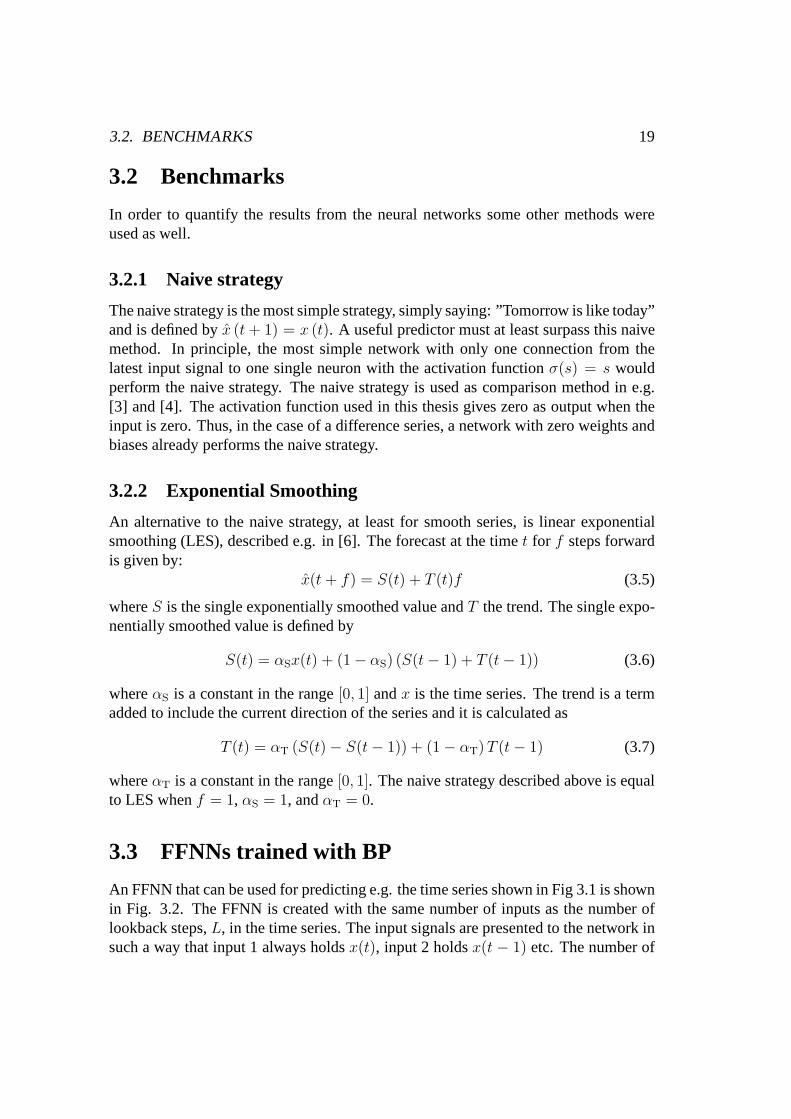
3.2.2 Exponential Smoothing

An alternative to the naive strategy, at least for smooth series, is linear exponentialsmoothing (LES), described e.g. in [6]. The forecast at the time t for f steps forwardis given by:

x(t + f) = S(t) + T (t)f (3.5)

whereS is the single exponentially smoothed value andT the trend. The single expo-nentially smoothed value is defined by

S(t) = αSx(t) + (1 − αS) (S(t − 1) + T (t − 1)) (3.6)

whereαS is a constant in the range[0, 1] andx is the time series. The trend is a termadded to include the current direction of the series and it iscalculated as

T (t) = αT (S(t) − S(t − 1)) + (1 − αT)T (t − 1) (3.7)

whereαT is a constant in the range[0, 1]. The naive strategy described above is equalto LES whenf = 1, αS = 1, andαT = 0.

3.3 FFNNs trained with BP

An FFNN that can be used for predicting e.g. the time series shown in Fig 3.1 is shownin Fig. 3.2. The FFNN is created with the same number of inputsas the number oflookback steps,L, in the time series. The input signals are presented to the network insuch a way that input 1 always holdsx(t), input 2 holdsx(t − 1) etc. The number of


x(t)

x(t − 1)

x(t − 2)

x(t − 3)

x(t − 4)

x(t + 1)

Fig. 3.2: An FFNN, with five neurons in the hidden layer, that estimates the time seriesx for time t + 1 given signals from timet − 4 to t.

neurons in the hidden layer,nh, is determined empirically for each case, but is typicallyaround 5. Whennh is chosen too large, the FFNN will overfit easily, i.e. the outputfrom the network will be very good when the training data set is predicted but worsefor the validation set, due to noise adaptation. On the otherhand, a too smallnh willlimit the capacity to a small number of different behaviors in the series. The constantβ, which is the same for all neurons in the FFNN used here, is typically 1. Initially,the weights in the network are all set randomly in the range[−1, 1]. When the FFNNis trained, the weights are updated after each input-outputpair (prediction). The input-output pairs are looped through in random order. The learning rate constantη0 wastypically about 0.02, while the learning time constant,τη, was set in the range5 · 104

to 2 · 106.

However, as mentioned in chapter 1, the FFNN has no short-term memory. Forinstance, in the example shown in Fig. 1.1, withL = 3, the inputs are identical forthe two series and the output from the FFNN will thus be identical irrespective ofearlier input signals. This is a built-in limitation of FFNNs which cannot be evaded nomatter what training algorithms are used. This problem can,of course, be solved byincreasingL but then the number of weights will grow too (the number of weights isequal tonh(L + 2) + 1), and this will increase the risk of overfittning and make thetraining of the network more computationally demanding. Besides, increasingL willnot solve the optimal design problem for the FFNN, i.e. the architecture of the networkstill has to be set beforehand. This is one of the main reasonsfor introducing the newmethod described in section 3.5.

3.4. RNNS TRAINED WITH GA 21

x(t)

x(t − 1)

x(t − 2)

x(t − 3)

x(t − 4)

x(t + 1)

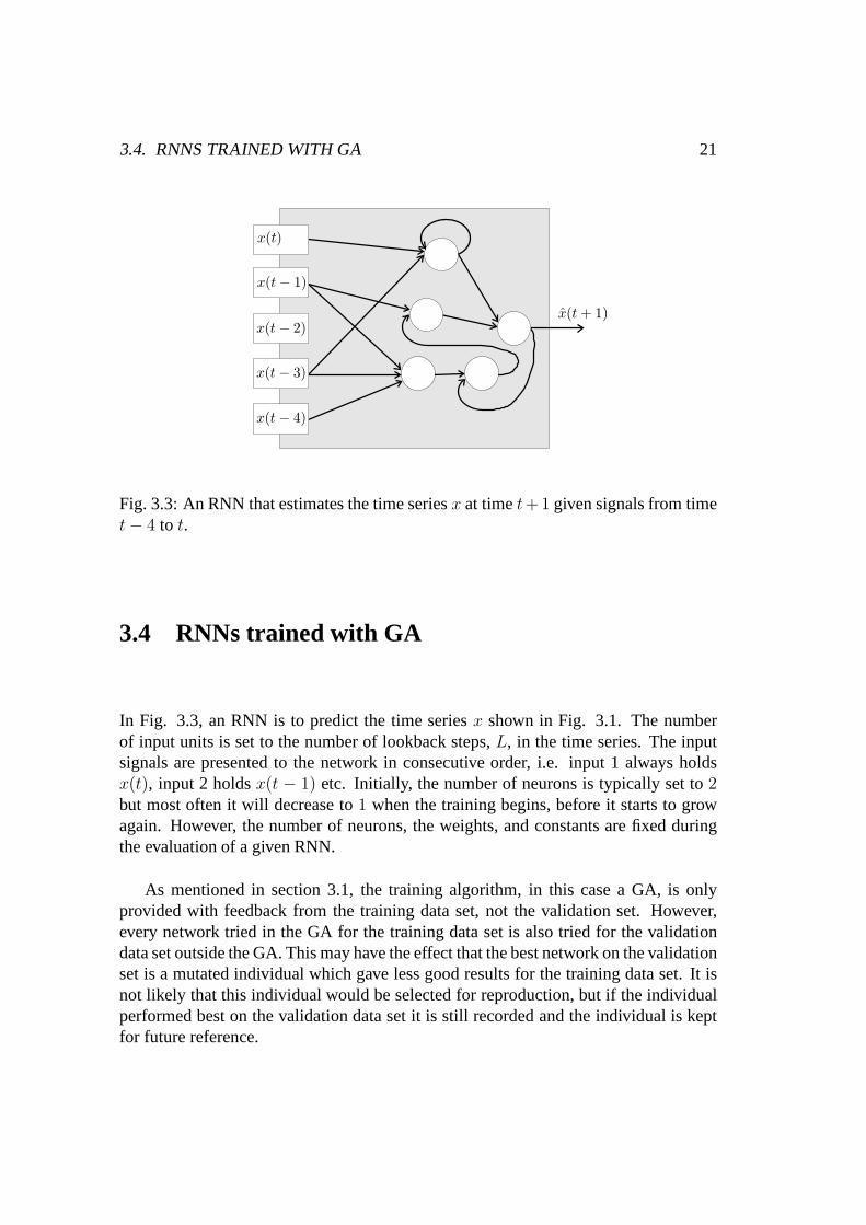
Fig. 3.3: An RNN that estimates the time seriesx at timet+1 given signals from timet − 4 to t.

3.4 RNNs trained with GA

In Fig. 3.3, an RNN is to predict the time seriesx shown in Fig. 3.1. The numberof input units is set to the number of lookback steps,L, in the time series. The inputsignals are presented to the network in consecutive order, i.e. input 1 always holdsx(t), input 2 holdsx(t − 1) etc. Initially, the number of neurons is typically set to2but most often it will decrease to1 when the training begins, before it starts to growagain. However, the number of neurons, the weights, and constants are fixed duringthe evaluation of a given RNN.

As mentioned in section 3.1, the training algorithm, in thiscase a GA, is onlyprovided with feedback from the training data set, not the validation set. However,every network tried in the GA for the training data set is alsotried for the validationdata set outside the GA. This may have the effect that the bestnetwork on the validationset is a mutated individual which gave less good results for the training data set. It isnot likely that this individual would be selected for reproduction, but if the individualperformed best on the validation data set it is still recorded and the individual is keptfor future reference.


x(t)

x(t − 1)

x(t − 2)

x(t − 3)

x(t − 4)

x(t + 1)

Fig. 3.4: An RNN, evolved from an FFNN, that estimates the time seriesx at timet+1given signals from timet− 4 to t. The likeness with the original FFNN, shown in Fig.3.2, is evident.

3.4.1 Fitness

The fitness value, needed for the EA (described in section 2.2), is defined by

F =1

E(3.8)

whereE is the root mean square error calculated as in Eq. 3.1.

3.5 RNNs generated from FFNNs

In this method, proposed in Paper I, an ANN is first initialized and trained with back-propagation as described above in section 3.3. The weights are then coded into achromosome (shown in Fig. 2.6) together with the constants:τ , β, andb. A popu-lation is formed from slightly mutated copies of this chromosome. Since the numberof genes is typically∼ 102, mutation in too many genes would, with high probability,destroy the performance of the original FFNN, even in the case of creep mutations. AGA, as described above, but with this initial population instead of a random one, isthen used for evolving RNNs. During the evolution, feedbackconnections are allowedif needed. An example is shown in Fig. 3.4. Compared to the FFNN in Fig. 3.2, newconnections have been formed and some of the old connectionshave been removed.

Chapter 4

Results

4.1 Introduction

In this chapter, results from the analysis of three different time series are reported,namely the USD-JPY exchange rate, the US unemployment rate,and the Dow JonesIndustrial Average.

The linear exponential smoothing method rarely gave betterresults than the naivemethod, i.e. the constantsαS andαT could be set 1 and 0, respectively. For this reason,the results from the LES method are not shown separately in the result tables.

4.2 Time series

4.2.1 USD-JPY exchange rate

The data set used consisted of weekly averages of the daily interbank exchange ratefrom US dollar (USD) to Japanese yen (JPY) between 1986 and 2003. It contained906 values, the unit of the values was Japanese yen, and the range was [82,164]. Theaveraging period eliminates weekly patterns.L was set to 4, which gave 902 values leftfor prediction, of which the first 539 were used for training and the remaining 363 forvalidation. For the difference series, the range was [-15,15] but the number of valuesused for training and validation was the same.

The RMS errors for both training and validation are shown in Table 4.1. The rela-tive improvements from the naive strategy are shown in Table4.2. The RNN obtainedfrom the best FFNN in an EA, i.e. using the method proposed here, and in Paper I,gave the best results. Compared to the FFNN, during the evolution this RNN improvedits results by 0.9% and 4.7% for the RMS validation and training error, respectively.The difference series in the exchange rate gave generally better results than the originalseries. Here, the RNN evolved from a random initial population performed best. How-

23

24 CHAPTER 4. RESULTS

Table 4.1: Results from several different time series. The second column shows thelookback length and the subsequent columns show the error (normalized to [0,1]),obtained for the naive strategy, FFNN, RNN, and finally RNN evolved with FFNN asinitial population. A ’d’ after the series number implies that the difference series wasused. Series I = USD - JPY interbank exchange rate, Series II =US Unemploymentrate, and Series III = DJIA.

S. L Naive FFNN RNN RNN f. FFNNTr. Val. Tr. Val. Tr. Val. Tr. Val.

I 4 0.0183 0.0213 0.0191 0.0208 0.0216 0.0208 0.0182 0.0206Id 0.0171 0.0207 0.0178 0.0203 0.0173 0.0204II 5 0.0275 0.0163 0.0233 0.0161 0.0234 0.0154 0.0228 0.0159IId 0.0229 0.0160 0.0251 0.0157 0.0243 0.0156III 5 0.0704 0.0564IIId 0.0677 0.0535 0.0675 0.0530 0.0673 0.0530

ever, the RNN evolved from an FFNN made an improvement of 1.6%for the RMSvalidation error but suffered a decrease of 1.2% for the RMS training value.

According to [12], in which ANNs are used on several different currencies, it isdifficult to forecast the trends in Japanese yen with technical algorithms. Their theoryis that the market for JPY is large and more efficient, and therefore acts quickly onsigns of change.

4.2.2 US unemployment rate

In this case the data set used consisted of monthly measurements of the US unem-ployment rate (seasonally adjusted), between January 1948and September 2003. Theseries consisted of 669 values, the unit was per cent (%), andthe range of the serieswas [2,11].L was equal to 5, the training set consisted of the first 442 values and thevalidation set the remaining 222. For the difference series, the range was [-1.5,1.5] andthe validation data set was one value shorter.

The RMS errors are shown in Table 4.1, and the relative improvements from thenaive strategy are shown in Table 4.2. For the original series, the best result camefrom the RNN evolved from a random population. The other RNN,evolved from theFFNN, improved (lowered) the RMS error with 1.89% and 1.68% during the evolutionfor the training and validation data set respectively. For the difference series the bestresult was obtained from the RNN evolved from the FFNN. During the evolution, thevalidation RMS error sank by 2.12%, but rose by 6.51% for the training set. However,

4.2. TIME SERIES 25

Table 4.2: Improvements from the naive method used for each series. A ’d’ after theseries number refers to the difference series. Series I = USD- JPY interbank exchangerate, Series II = US Unemployment rate, and Series III = DJIA.

Series FFNN RNN RNN from FFNNTr. Val. Tr. Val. Tr. Val.

I -3.92% 2.20% -17.53% 1.93% 0.94% 3.12%Id 6.90% 2.42% 2.77% 4.39% 5.79% 4.01%II 15.52% 1.19% 14.95% 5.50% 17.11% 2.84%IId 17.02% 2.04% 8.71% 4.09% 11.62% 4.12%IIId 3.89% 5.08% 4.11% 6.01% 4.50% 5.89%

it should be noted that the FFNNs were only able to achieve a good fit for the trainingdata set. Overall, the validation data set showed differentbehavior to the training dataset, which can be seen in the results of the naive method. The RMS error for thetraining data set is almost 70% larger than the validation error.

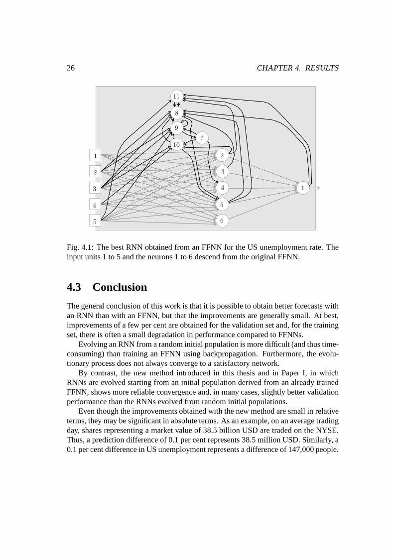
The best RNN obtained from an FFNN is shown in Fig. 4.1.

4.2.3 Dow Jones Industrial Average

The series used is based on the average of 22 trading days (about a month) of dailyDow Jones Industrial Average (DJIA) closings from 1928 to 2003. Because of theincreasing trend of the data set the series was transformed into a difference seriesaccording to

xd(t) =x(t + 1) − x(t)

x(t), t = 1, . . . , (m − 1) (4.1)

The series consisted of 905 values in the range [-0.3,0.4].L was equal to 5, 600 valueswere used for training, and 300 values were used for validation.

The RMS values are shown in Table 4.1, and the relative improvements from thenaive strategy are shown in Table 4.2. The result from the naive method is calculatedfrom the original series. The best result came from the RNN evolved from a randompopulation. The other RNN, evolved from the FFNN, improved (lowered) the RMSerror by 0.64% and 0.86% for the training and validation datasets, respectively.

26 CHAPTER 4. RESULTS

1

1 2

2

3

3

4

4

5

5

6

7

8

9

10

11

Fig. 4.1: The best RNN obtained from an FFNN for the US unemployment rate. Theinput units 1 to 5 and the neurons 1 to 6 descend from the original FFNN.

4.3 Conclusion

The general conclusion of this work is that it is possible to obtain better forecasts withan RNN than with an FFNN, but that the improvements are generally small. At best,improvements of a few per cent are obtained for the validation set and, for the trainingset, there is often a small degradation in performance compared to FFNNs.

Evolving an RNN from a random initial population is more difficult (and thus time-consuming) than training an FFNN using backpropagation. Furthermore, the evolu-tionary process does not always converge to a satisfactory network.

By contrast, the new method introduced in this thesis and in Paper I, in whichRNNs are evolved starting from an initial population derived from an already trainedFFNN, shows more reliable convergence and, in many cases, slightly better validationperformance than the RNNs evolved from random initial populations.

Even though the improvements obtained with the new method are small in relativeterms, they may be significant in absolute terms. As an example, on an average tradingday, shares representing a market value of 38.5 billion USD are traded on the NYSE.Thus, a prediction difference of 0.1 per cent represents 38.5 million USD. Similarly, a0.1 per cent difference in US unemployment represents a difference of 147,000 people.

Bibliography

[1] C. DARKEN, J. CHANG, AND J. MOODY, Learning Rate Schedules for FasterStochastic Gradient Search, in Neural Networks for Signal Processing 2 - Pro-ceedings of the 1992 IEEE Workshop, New Jersey, 1992, IEEE Press.

[2] R. DAWKINS, The Selfish Gene, Oxford University Press, New York, 1976.

[3] C. L. DUNIS AND M. W ILLIAMS , Modelling and Trading the EUR/USD Ex-change Rate: Do Neural Network Models Perform Better?, Derivatives Use,Trading and Regulation, 8 (2002), pp. 211–239.

[4] C. L. GILES, S. LAWRENCE, AND A. C. TSOI, Noisy Time Series PredictionUsing a Recurrent Neural Network and Grammatical Inference, Machine Learn-ing, 44 (2001), pp. 161–183.

[5] S. HAYKIN , Neural Networks, A Comprehensive Foundation, Prentice Hall, NewJersey, second edition, 1999.

[6] S. MAKRIDAKIS AND S. C. WHEELWRIGHT, Forecasting Methods for Manage-ment, Wiley, New York, fifth edition, 1989.

[7] J. E. MOODY, Economic forecasting: Challenges and neural network solutions,in Proceedings of the International Symposium on ArtificialNeural Networks,Hsinchu, Taiwan, 1995.

[8] J. PETTERSSON ANDM. WAHDE, Generating balancing behavior using recur-rent neural networks and biologically inspired computation methods. Submittedto IEEE Transactions of Evolutionary Computation, September 2003.

[9] M. WAHDE, An Introduction to Adaptive Algorithms and Intelligent Machines,Goteborg, Sweden, second edition, 2002.

[10] P. WERBOS, Backpropagation through time: what it does and how to do it, Pro-ceedings of the IEEE, 78 (1990), pp. 1550–1560.

27

28 BIBLIOGRAPHY

[11] R. J. WILLIAMS AND D. ZIPSER, A Learning Algorithm for Continually Run-ning Fully Recurrent Neural Networks, Neural Computation, 1 (1989), pp. 270–280.

[12] J. YAO, H.-L. POH, AND T. JASIC, Foreign Exchange Rates Forecasting withNeural Networks, September 1996, pp. 754–759.

[13] X. YAO, Evolving Artificial Neural Networks, Proceedings of the IEEE, 87(1999), pp. 1423–1447.

IMPROVING TIME SERIES PREDICTION USING RECURRENT NEURAL NETWORKS

Documents

Transcript of IMPROVING TIME SERIES PREDICTION USING RECURRENT NEURAL NETWORKS