Improving paired comparison models for NFL point spreads

by data transformation

by

Gregory J. Matthews

A Project Report

Submitted to the Faculty

of

WORCESTER POLYTECHNIC INSTITUTE

in partial fulfillment of the requirements for the

Degree of Master of Science

in

Applied Statistics

by

May 2005

APPROVED:

Jayson D. Wilbur, Advisor

Bogdan M. Vernescu, Department Head

Acknowledgements

Special thanks to Jayson Wilbur for taking over as my advisor late in the project

and not holding meetings before noon. Further thanks go out to Carlos Morales for

advising the project in its early stages.

I’d like to all my fellow graduate students for all of their help over my years here.

Thanks to Erik Erhardt for his sage advice to always sum the residuals. Special

thanks to Shawn Hallinan for suffering through 540 and 541 with me and always

keeping a fair score.

JOC.

Thank you Professor Petruccelli. Thanks to Andrew Swift: tough break being a

Dolphins fan though.

Thank you to the entire math department especially for the financial support.

Abstract

Each year millions of dollars are wagered on the NFL during the season. A few

people make some money, but most often the only real winner is the sports book.

In this project, the effect of data transformation on the paired comparison model

of Glickman and Stern (1998) is explored. Usual transformations such as logarithm

and square-root are used as well as a transformation involving a threshold. The

motivation for each of the transformations if to reduce the influence of “blowouts” on

future predictions. Data from the 2003 and 2004 NFL seasons are examined to see if

these transformations aid in improving model fit and prediction rate against a point

spread. Strategies for model-based wagering are also explored.

Contents

1 Introduction 1

1.1 Background . . . . . . . . . . . . . . . . . . . . . . . . . . . . . . . . 1

1.2 Data description . . . . . . . . . . . . . . . . . . . . . . . . . . . . . 4

1.3 Bradley-Terry paired comparison model . . . . . . . . . . . . . . . . . 5

1.4 Modeling point difference . . . . . . . . . . . . . . . . . . . . . . . . . 6

2 Methods 8

2.1 Bayesian hierarchical model for point difference . . . . . . . . . . . . 9

2.2 Data transformations . . . . . . . . . . . . . . . . . . . . . . . . . . . 12

2.3 Convergence diagnostics . . . . . . . . . . . . . . . . . . . . . . . . . 15

2.4 Model evaluation . . . . . . . . . . . . . . . . . . . . . . . . . . . . . 16

3 Application to 2003 and 2004 NFL Data 18

3.1 Data . . . . . . . . . . . . . . . . . . . . . . . . . . . . . . . . . . . . 18

iv

3.2 Diagnostics . . . . . . . . . . . . . . . . . . . . . . . . . . . . . . . . 19

3.3 Results . . . . . . . . . . . . . . . . . . . . . . . . . . . . . . . . . . . 24

4 Model Based Strategy 28

4.1 Credible intervals . . . . . . . . . . . . . . . . . . . . . . . . . . . . . 28

4.2 Home versus visitor . . . . . . . . . . . . . . . . . . . . . . . . . . . . 30

4.3 Underdog versus favorite . . . . . . . . . . . . . . . . . . . . . . . . . 34

4.4 Other selection methods . . . . . . . . . . . . . . . . . . . . . . . . . 35

5 Conclusions 41

5.1 Recommendations . . . . . . . . . . . . . . . . . . . . . . . . . . . . . 41

5.2 Summary and future work . . . . . . . . . . . . . . . . . . . . . . . . 42

v

List of Figures

2.1 Signed-log transformation . . . . . . . . . . . . . . . . . . . . . . . . 14

2.2 Adjusted signed-log transformation . . . . . . . . . . . . . . . . . . . 14

2.3 Signed-square-root rransformation . . . . . . . . . . . . . . . . . . . . 15

3.1 Autocorrelation of Gibbs sampler for posterior predictive distribution

of the point difference for a game in week 17 . . . . . . . . . . . . . . 20

3.2 History from a game in week 17: New England versus San Francisco . 20

3.3 History from a game in week 17: Minnesota versus Washington . . . 20

3.4 Mean squared prediction error (MSPE) versus threshold value . . . . 21

4.1 Home Field Advantage versus week for 2003 and 2004 . . . . . . . . . 39

4.2 Strength parameter estimates of teams in 2003 . . . . . . . . . . . . . 39

4.3 Strength parameter estimates of teams in 2004 . . . . . . . . . . . . . 40

vi

List of Tables

3.1 Convergence diagnostics for the Gibbs sampler . . . . . . . . . . . . . 19

3.2 Statistical performance measures for different thresholds in 2003 . . . 22

3.3 Statistical performance measures for different thresholds in 2004 . . . 23

3.4 Statistical performance measures of certain data transformations models 26

3.5 Prediction performance measures of certain data transformed models 26

3.6 Statistical performance measures for different thresholds models through

2003 and 2004 . . . . . . . . . . . . . . . . . . . . . . . . . . . . . . . 27

4.1 Profit over 2003 and 2004 NFL seasons betting 110 to win 100 using

different intervals as selection methods . . . . . . . . . . . . . . . . . 31

4.2 Prediction rate using credible intervals to select games to bet with

number of games in parenthesis . . . . . . . . . . . . . . . . . . . . . 32

4.3 Profit over 2003 and 2004 NFL seasons betting 110 to win 100 home

versus away . . . . . . . . . . . . . . . . . . . . . . . . . . . . . . . . 33

vii

4.4 Profit over 2003 and 2004 NFL seasons betting 110 to win 100 underdog

versus favorite . . . . . . . . . . . . . . . . . . . . . . . . . . . . . . . 36

4.5 Profit over 2003 and 2004 NFL seasons betting 110 to win 100. Model

chooses underdog to win game outright and games are bet against the

spread . . . . . . . . . . . . . . . . . . . . . . . . . . . . . . . . . . . 38

4.6 Using two selection methods to choose games . . . . . . . . . . . . . 40

viii

Chapter 1

Introduction

1.1 Background

Since the beginning of organized sports in America, people have bet on the outcome

of games. Sports betting began to grow rapidly in the early part of the 20th century

as the popularity of college football and basketball increased. Today, gambling is in

a golden era. The Nevada sports gambling industry had revenues of almost 2 billion

dollars last year, and it is estimated that revenues for the internet sports betting

industry were 63 billion dollars. [1]

Each year, a large portion of that money is wagered on the National Football League

(NFL) during the course of a season, culminating in the greatest sports gambling

event of the year, the Super Bowl. It is estimated that one in four men and one in

eight women wager money on the Super Bowl in one form or another.

A few people make some money, but more often the only real consistent winners are

the companies who make the odds for the game, called sports books. Most of these

1

people betting on the NFL with sports books rely solely on intuition when making

their picks. What if point differences could be modeled using statistical techniques?

When people first started to gamble on sporting events they simply bet on which

team they thought would win the game outright. If one team was favored to win,

most bettors would bet on this team causing a lopsided distribution of the money

being wagered on each side of a game. Thus bettors had to risk a lot of money for a

small gain. Likewise, if a team was perceived to be likely to lose a given game, the

bettor would win more than he risked if the team prevailed. Often times, however,

one team was so much more likely than the other team to win a given game, a sports

book risked incurring a huge loss if a heavy favorite lost, since all of the money bet

on the game was bet on the same team.

The solution to this problem was something called a point spread which first appeared

in the 1940s. [1] The point spread is a system in which the perceived stronger team,

often called the “favorite,” is given a handicap. The handicap is a certain number

of points subtracted from the favorite’s final score. This could also be viewed as the

weaker team, often called the underdog, having points added to their score. Under

the point spread system, the bettor wins if the team he bet on has a higher score at

the end of the game after the specified handicap has been added.

For example, if a bet were placed on Team A +9, Team A is said to be “getting nine

points.” This bet is a winner if Team A either wins the game outright or loses by

less than nine points. Alternatively, if a bet were placed on the favored Team B -9,

Team B is said to be giving nine points. This second bet is a winner if Team B wins

the game by more than nine points and they are said to have “covered the spread.”

In either example, if Team B won by exactly nine points, the game is said to be a

“push,” and all bets are returned to the bettors. Frequently, a point spread will have

2

half points (i.e. +9.5). This prevents push situations previously mentioned. A half

point in the right direction is often very advantageous to the bettor (or sports book).

In most cases, when betting against a point spread, the bettor must risk slightly

more than he would win if he picks correctly. This extra amount that is risked

enables sports books make a profit. Frequently, a bet is made risking 11 units to

win 10. Almost always bets against a point spread have these odds, which are often

refered to as either “11/10,” or “-110.” (There are sports books on the internet that

offer bets against the point spread with odds of 21/20, or -105, but 11/10 is more

common.) This gives a gambler a number to shoot for: 52.381 percent. If winners are

correctly chosen at exactly this percentage, the gambler would break even. Correctly

predicting winners in excess of this number will result in a profit, while falling short

of this number results in a loss. Most times, people are unable to consistently predict

winners in excess of this target percentage and incur losses. To be profitable in the

long run, a gambler just needs to be better than the point spread approximately 53

out of 100 times.

How exactly are point spreads decided upon before the start of a game? Sports books

are not in the business to gamble. They want to be guaranteed to make money no

matter what happens. The purpose of a point spread is to divide the money bet on

a given game so that an acceptable amount of money is on each side of the spread.

Then, regardless of the outcome, winners are paid out at 11/10 and the sports book

makes money. Point spreads are not meant to be predictions of a given sporting event,

they merely reflect public opinion. As a result of this, if a bettor can outwit public

opinion more than 52.381 percent of the time, a long term profit can be made. The

fact that a bettor can place bets against other people is what makes betting on sports

so appealing as a long term profitable form of gambling.[2] Simply put, to profit in

the long term, one must be a better bettor than the average person.

3

1.2 Data description

In this project, the regular season data from the 2003 and 2004 NFL seasons will

be examined. There are 256 regular season games in each NFL season spread over

seventeen weeks. In weeks one and two all of the thirty-two teams plays, for a total

of sixteen games. In weeks three through ten there are fourteen games, as four teams

each week get a bye during this time. In weeks eleven through seventeen all teams

resume playing every weekend for a total of sixteen games per week. [3]

Each regulation-length game in the NFL season consists of four quarters of fifteen

minutes each. The team with more points at the end of the four quarters is the winner.

If the score is tied at the end of regulation, there is an overtime period. Overtime

in the NFL consists of one fifteen minute period with the first team to score in the

overtime being declared the winner. If no team scores in the overtime before time

expires, the game is declared a tie.

It is believed that an important factor in modeling point spreads is information about

where the game is played. This leads to a concept of home field advantage in many

sports. On average, the home team wins more often than the visiting team. Previous

studies have estimated the size of this effect in the NFL to be approximately three

points. [4] Three points is very often the difference between a win and a loss against

the spread. So home field advantage is a very important factor to consider in any

model attempting to model point difference.

4

1.3 Bradley-Terry paired comparison model

The Bradley-Terry model [5] is a generalized linear model for paired comparisons.

Paired comparison models are useful because people have difficulty ordering several

items, but are able to choose between two items very easily. Such models use infor-

mation about pairwise comparisons to enable inference about the relative ranking of

all items under consideration. A simple application of the Bradley-Terry model is

in taste tests. It may be difficult to give an order of preference for several different

foods, but quite easy to choose a preference between any pair of items. If one item

is chosen over another item, it might be considered a “win” for that item and based

on a large enough quantity of paired comparisons, a ranking of the foods could be

produced.

Another motive for using a paired comparison model, such as the Bradley-Terry

model, is for ranking teams in sports. One can use this ranking to try to predict the

outcome of future games by objectively evaluating the strengths of the two teams

involved in the game. If there was enough information about who was going to win

a game, one could bet accordingly and gain a profit. However, betting just wins and

losses may not be a very good way to make money in the long run. If a team is

heavily favored to win a game one may have to risk hundreds of dollars just to try to

win one hundred.

The Bradley-Terry model can be described as follows. Let βi denote the strength

parameter of team i and βj denote the strength parameter of team j. Given two

competing teams i and j it can be said that

Pij = f(βi, βj)

5

where Pij is the probability that team i defeats team j. The logit link function is

commonly used because the range of Pij is restricted to [0, 1].

logit(Pij) = log

(Pij

1− Pij

)

Since, 1− Pij = Pji this leads to

logit(Pij) = log

(PijPji

).

This link function is used to allow the parameters to vary on the range (−∞,∞).

Now the parameters can take on all values in the domain of a normal random variable

and can be modeled by

logPij

1− Pij= βi − βj

where βi and βj represent the individual strengths of team i and j respectively. From

the previous equation it follows that

Yij ∼ Bernoulli(Pij)

As a matter of practice, one team’s strength parameter is assigned to be exactly zero,

and all estimates made relative to the assigned team. If no such constraint is used,

the design matrix is not of full rank and paramters are not estimable.

1.4 Modeling point difference

In its simplest form, Bradley-Terry only takes into account wins and losses. That

simple model predicts winners of games very well, while only using a small amount

6

of information. However, it does very little in the way of giving estimates for the

margin of victory. For this, rather than just using data for a win or a loss, the model

becomes

Yijk = βi − βj + εijk

where Yijk is the margin of victory in a game in the kth week between team i and

team j.

Rather than being an overall estimate of a teams ability to win, the team strength

parameters now represent the ability to score points in excess of the team whose pa-

rameter has been set to zero. This reduces to a classic regression model with indicator

variables for the teams involved in the game with the data and errors assumed to be

normally distributed.

In a Bayesian context the same model can be used, however, now priors on the

strength and variance parameters are added. The advantage of Bayesian estimation is

that reasonable estimates can be made with less data than required by the frequentest

approach. Furthermore, when not using Bayesian estimation, parameters of teams

that are undefeated or winless are estimated as infinite. The shrinkage induced by

Bayesian estimation pulls these estimates closer to zero, and they tend to be more

realistic.

7

Chapter 2

Methods

In this project, point spreads will be modeled as a function of the two teams involved

in the game and where the game is being played. The strength parameters of each

team and the home field advantage parameter will be estimated and allowed to vary

over time to account for variability over the course of a season. These estimations

will then be used to predict the outcome of future games. Predictions for week k

are made by estimating all parameters using data from weeks 1 through week k − 1

and taking draws from the posterior predictive distribution of each game in week k.

Predictions are made for weeks four through seventeen in the 2004 season, and for

weeks three through seventeen for the 2003 season. These weeks are omitted from

prediction because it is assumed that there is not enough data from the season in the

early weeks.

8

2.1 Bayesian hierarchical model for point differ-

ence

Let ygk denote the margin of victory for the favorite in game g of week k. Note that

ygk is negative in the event that the home team loses the game. Game g is played

between two teams gh and ga, with gh being the index of the home team and ga being

the index of the away team. βk is a vector of all team strength parameters at week k,

thus βghk denotes element of βk corresponding to the home team in game g. Likewise,

βgak corresponds to the away team in game g of week k. The parameter αk is the size

of the home field advantage in week k. It is assumed to be the same for all teams,

but is allowed to vary over the course of the season. This gives the model

ygk = βghk − βgak + αk + εgk

Therefore, the distribution of scores from week k is

ygk|µgk, σ2 ∼ N(µgk,

1

σ2

)

and

µgk =32∑m=1

(Xgkmβmk) + αk

which reduces to

µgk = βghk − βgak + αk

where gh and ga range from 1 to 31.

Here X is the Gk × 33 design matrix, where Gk is the total number of games played

through week k, with each row representing one game of the NFL season defined as

9

Xgkm =

1 if team m is home in game g of week k

−1 if team m is away in game g of week k

0 otherwise

The first thirty-two columns of the matrix represent each of the NFL teams and the

thirty-third column represents home field advantage. In each row of X there is a 1 in

column i for the home team and a −1 in column j for the visiting team. There is a

column of 1’s representing the home field advantage in the thirty-third column of X.

The prior distributions assumed for the team strength parameters and home field

advantage parameters can be expressed by

βmk|φ, βm,k−1, ζ2 ∼ N

(φββm,k−1,

1

ζ2

)

and

αk|φ, αi,k−1, ψ2 ∼ N

(φααk−1,

1

ψ2

)

[4].

In general, the φs are autoregressive parameters on the interval [−1, 1]. In this case,

for simplicity, we let φα = φβ = 1. By choosing this specific value for the φs, the

AR(1) process reduces to a random walk in the parameter space. This above set up

allows for the individual team strength parameters to vary over time over the course

of a season.

The prior distributions assumed for the precision parameters on ζ2, ψ2, σ2 are all

χ25. These distributions are chosen because they are the conjugate priors. To try

to be as non-informative as possible, widely dispersed distributions corresponding

10

to very few degrees of freedom are chosen. Computationally the algorithm used in

WinBUGS [6], the Gibbs sampler [7], has trouble converging if the distribution is too

widely dispersed. Five degrees of freedom are used to satisfy both a widely dispersed

distribution and allows for WinBUGS to run.

Initial values for βg0 are drawn from N(0, 1

ζ2

)and α0 is drawn from N

(0, 1

ψ2

)The joint posterior distribution for the model parameters is

π(βgk, αk, σ2|Y ) ∝ f(Y |βgk, αk, σ2, X)π(βgk, αk, σ

2, X)

and can also be written

π(βgk, αk, σ

2|Y ) ∝ f(Y |βgk, αk, σ2, X)π(βgk|ζ2)π(αk|ψ2)π(ψ2)π(ζ2)π(σ2)

WinBUGS [6] uses the Gibbs sampler to enable posterior inference of the parameters.

[7]

It should be noted that in football, score differences take on only integer values. In

addition, because of the scoring rules in football some values are more likely than

others. As a result of the increment in which points are scored in football, (3 for

a field goal and 7 for a touchdown) some margins of victory occur more often than

others. For instance, games are won more often by 3 then by 1. However, in this

model it is assumed that point differences follow a normal distribution. Glickman

[8] cites many sources claiming that the normality assumption is not unreasonable

[9, 10, 11].

11

2.2 Data transformations

Several data transformations were explored to see if it would aid in reduction of model

error or increase the prediction rate of games, both against the spread and outright.

A signed-square-root model and two different signed-log models were used, as well

as a threshold model, which is explained below, to model the point spread. The

motivation here is to try to reduce the effect of large victory margins. It is believed

that when a team wins a game by a very large number of points, there is very little

information in the last points gained. Often times, near the end of a game that is

being won by a large amount of points the losing team will remove its best players,

as to try to avoid injuring themselves at a meaningless part of the game.

The two forms of the signed-log transformation that are considered are, first, a regular

signed-log transform. This makes the new model

sign(ygk)log(|ygk|) ∼ N(µgk, σ2)

with µgk = βghk − βgak + αk. After the parameters are estimated an inverse trans-

formation is employed to so that inference can be made on the original scale. This

causes problems, however, because the signed-log transformation is not monotone

(See Figure 2.1.).

To alleviate this problem an adjusted transformation is suggested. The adjusted

signed-log model is

sign(ygk) log(|ygk|+ 1) ∼ N(µgk, σ2)

where µgk = βghk − βgak + αk. The form of this transformation can be seen in Figure

2.2.

12

Also considered is the signed-square-root model having the form

sign(ygk)√|ygk|+ 1 ∼ N(µgk, σ

2)

where, same as the first two, µgk = βghk − βgak + αk. This transformation can be

viewed is figure 2.3

While all of these models try to accomplish the same goal of reducing the effect of

large margins of victory on future predictions, the signed square-root transformation

allows for slightly larger margins of victory than its log counterpart. This is achieved

by the square-root increasing faster than the signed-log transformations.

The threshold model is a little bit different. If a team wins by less than a threshold

value Ψ, the entire victory margin is considered and no transformation is made. If a

team wins by more than the threshold we map the actual out come to the threshold

value, so that all values greater than the threshold equal the threshold. This results

in the model

g(ygk) = βghk − βgak + αk + εgk

where

g(ygk) =

ygk if ygk ≤ Ψ

Ψ if ygk ≥ Ψ

All of these data transformations try to serve the same purpose. They are trying to

decrease the impact of a large victory, or blowout.

13

Figure 2.1: Signed-log transformation

Figure 2.2: Adjusted signed-log transformation

14

Figure 2.3: Signed-square-root rransformation

2.3 Convergence diagnostics

Whenever using Markov chain Monte Carlo (MCMC) methods to make inference, it

is important to check whether or not the Markov chain has converged to a stationary

distribution, namely, the posterior distribution. This is difficult, however, because

the estimates produced by the algorithm are not a single number nor a distribution,

but a sample from a distribution. Some sort of test is needed to decide upon whether

the algorithm is producing results that are stationary. There are many different

diagnostics used to test for convergence. [12]

Geweke’s convergence diagnostic [13] is based on the difference of the mean of the first

nA iterations and the mean of the last nB iterations. If this difference is divided by the

asymptotic standard error, this statistic has a standard normal distribution. Geweke

suggests that nA = 0.1n and nB = 0.5n where n is the total number of iterations.

15

The Gelman-Rubin [14] diagnostic estimates the factor by which the scale parameter

might shrink if sampling were continued indefinitely. Convergence is monitored by

the test statistic√R =

√√√√(n− 1

n+m+ 1

mn

B

W

)(df

df − 2

)

where B denotes the variance between means, W denotes the average of the with-in

chain variance, m is the number of parallel chains, with n iterations, and df is the

degrees of freedom estimating the t density. The calculated value of√R should be

near one if the chain converges.

The Raftery-Lewis diagnostic [15] is meant to detect convergence of the stationary

distribution. It can also be used to provide a bound of the variance estimates of

quantiles of functions of parameters. This estimates the quantile q, to a desired

accuracy r.

2.4 Model evaluation

Several different methods were used for evaluating how well each model performed.

Mean squared prediction error (MSPE) and mean absolute prediction error (MAPE)

between predicted outcomes and actual outcomes is the first basic measure. They are

defined as

MSPE =∑gk

(ygk? − ygk)

2

N

and

MAPE =∑gk

|(ygk? − ygk)|N

where y?gk is the predicted margin of victory, ygk is the actual margin of victory, and

N is the total number of games for which predictions are made. A low MSPE or

16

MAPE indicates that the model is predicting close to actual game outcomes.

Other methods used to evaluate the models are prediction rate against the points

spread and prediction rate of outright winners. The model is said to correctly pick a

winner if the sign of predicted point difference is the same as the sign of the actual

outcome. Similarly, the model is said to correctly predict against the spread if the

predicted margin of victory and the actual outcome are both on the correct side of

the point spread.

17

Chapter 3

Application to 2003 and 2004 NFL

Data

The primary motivation for modeling point difference in the NFL is to try to accu-

rately predict future margins of victory. By modeling point difference, a bettor can

compare model-based predictions to announced point spreads. If predictions against

the spread could be made correctly in excess of the target percentage, 52.381 percent,

a profit could be made in the long run. Other motivating factors for this model are

to pick winners and losers of games, rather than picking against a point spread.

3.1 Data

The model proposed in Chapter 2, will be evaluated using data from the 2003 and

2004 NFL seasons. Data were collected on which teams were involved in each game

and where the game was played. Also collected were the points scored by each team

18

Test Outcome Convergence ConvergenceCriteria Indicated

Raftery and Lewis M=2 Starting iteration > M Yes

Gelman and Rubin√R̂ = 1 Values near 1 Yes

Geweke G1 = −.3441 |G| < 1.96 YesG2 = −.9748

Table 3.1: Convergence diagnostics for the Gibbs sampler

and the announced point spread of each game prior to its start. Since point spreads

may change as the week progresses, the point spread data used here are point spreads

from the time closest to the start of the game. The largest margin of victory in 2004

was 46 points and in 2003 it was 42 points. However, the margin of victory is small

for most games with 146 out of 256 games decided by ten or fewer points in 2003 and

145 out of 256 in 2004. The number of games decided by thirty or more points were

small by comparison, numbering 15 and 9 for the years 2003 and 2004 respectively.

There were no ties in either year, but this would be denoted as a margin of victory

of zero.

3.2 Diagnostics

The Bayesian hierarchical model proposed in Chapter 2, was fit using the software

package WinBUGS [6] which uses a Gibbs sampler when conjugate prior distributions

are used, as they are here. The convergence diagnostics discussed in Section 2.3 were

applied and the results are presented in Table 3.1. Both chains indicated convergence

happens almost immediately, as the burn-in number recommended by the Raftery-

Lewis diagnostic is only M = 2.

19

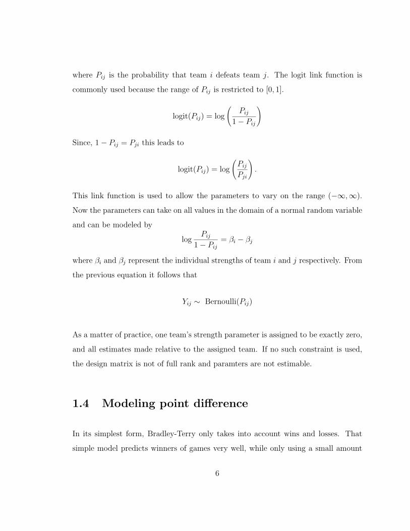
Figure 3.1: Autocorrelation of Gibbs sampler for posterior predictive distribution ofthe point difference for a game in week 17

Figure 3.2: History from a game in week 17: New England versus San Francisco

Figure 3.3: History from a game in week 17: Minnesota versus Washington

20

Figure 3.4: Mean squared prediction error (MSPE) versus threshold value

In terms of model fit, the threshold model outperformed the non-transformed data.

For successively larger values of the threshold, the error reduces quickly, then obtains

some minimum, after which it begins to increase again. This can be seen in figure

3.4. The minimum mean squared prediction error occurs at a threshold of 13 in 2003

and a threshold of 20 in 2004. All of the values can be seen in Tables 3.2 and 3.3

respectively. It should be noted, however, that the values for the errors between

about eleven and twenty-two are all very close in value. The non-transformed data

had a mean squared prediction error (MSPE) of 188.44 and in 2003 and 205.24 in

2004, whereas the threshold data obtains a minimum MSPE of 184.681 and 193.144

for 2003 and 2004 respectively. Both are improvements over the raw score difference.

This shows that by using a very low threshold, say five, not enough information is

being used in the model, and predictions suffer. On the other hand, if raw score data

is used, the very large values over-inflate the strength parameters of teams with very

large margins of victory. It appears that if a team is winning by any more than about

21

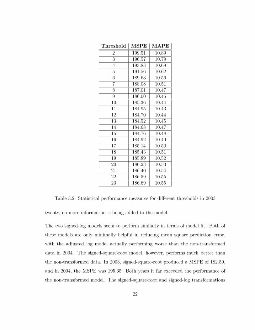
Threshold MSPE MAPE

2 199.51 10.893 196.57 10.794 193.83 10.695 191.56 10.626 189.63 10.567 188.08 10.518 187.01 10.479 186.00 10.4510 185.36 10.4411 184.95 10.4312 184.70 10.4413 184.52 10.4514 184.68 10.4715 184.76 10.4816 184.92 10.4917 185.14 10.5018 185.43 10.5119 185.89 10.5220 186.23 10.5321 186.40 10.5422 186.59 10.5523 186.69 10.55

Table 3.2: Statistical performance measures for different thresholds in 2003

twenty, no more information is being added to the model.

The two signed-log models seem to perform similarly in terms of model fit. Both of

these models are only minimally helpful in reducing mean square prediction error,

with the adjusted log model actually performing worse than the non-transformed

data in 2004. The signed-square-root model, however, performs much better than

the non-transformed data. In 2003, signed-square-root produced a MSPE of 182.59,

and in 2004, the MSPE was 195.35. Both years it far exceeded the performance of

the non-transformed model. The signed-square-root and signed-log transformations

22

Threshold MSPE MAPE

2 208.52 11.483 206.05 11.384 203.99 11.315 202.17 11.246 201.14 11.227 199.88 11.198 198.41 11.159 197.27 11.1310 196.32 11.1111 195.54 11.0912 194.92 11.0913 194.42 11.0914 194.09 11.0915 193.89 11.1016 193.72 11.1217 193.60 11.1318 193.29 11.1419 193.16 11.1420 193.14 11.1621 193.31 11.1722 193.42 11.1723 197.65 11.29

Table 3.3: Statistical performance measures for different thresholds in 2004

23

act in a manner similar to the threshold model. They do very little to change scores

close to zero, while down-weighting the score difference for large values. Intuitively

this seems to be a better alternative to the threshold model because the monotonicity

of the scores is maintained.

3.3 Results

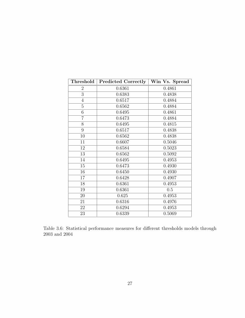
Percentage of wins correctly predicted and percentage of wins against the spread

are used as performance measures for each model. For 2003, the threshold model

predicted between 61.61 and 67.86 percent of outright winners of 224 games from

weeks three through seventeen. In 2004 the numbers ranged from 62.05 and 65.18

percent for the same number of games over the same time period. Over this same

period, with no transformation, 64.29 percent of winners were chosen in 2003 and

61.61 percent in 2004. The values for all the thresholds can be seen in Table 3.6

The other models performed very well when predicting winners. In 2003 the signed-

square-root model picked the most winners correctly, at 67.00 percent, and in 2004

adjusted signed-log model predicted 65.63 percent of games correctly. All three of

these transformations outperformed the untransformed model in prediction probabil-

ity as evidenced in Table 3.5.

Prediction percentage against the point spread was used as a final measure of perfor-

mance of the model. In 2003, the prediction against the spread was maximized by a

threshold at 5 points. This model correctly predicted 48.21 percent of games against

the spread from week three to seventeen for a total of 224 games. The lowest rate

of prediction in this same year came at threshold values of 8 and 9. Both thresholds

predicted 45.98 percent of games. The raw data for 2003 correctly predicted 106

24

games for a prediction rate of 47.32 percent. These number show just how difficult it

is to predict against the spread in the NFL.

In 2004, the predictions against the spread faired much better. Out of 210 games

from weeks four through seventeen, the threshold value that maximized prediction

against the spread was 13 points. At this value, 116 games were correctly picked at a

rate of 55.23 percent. The threshold model did the worst for this year at 2, 5, and 6.

For all of these threshold values the prediction rate was 49.52 percent. The prediction

rate for the raw data model in 2004 was 50.48 percent.

These rates against the spread are discouraging, and further indicate just how difficult

picking against the spread can be. In some instances, one may be better off just

flipping a fair coin. However, for both years prediction of the spread is improved

when using square-root and both log models. In 2003, the natural log model is the

only model that predicts over half of the games against the spread, at a rate of

50.45 percent, with the other two models are not far behind. The square-root model

predicts 49.55 percent and the adjusted signed-log model predicts 49.11 percent. Both

are marked improvements over the raw data model and all of the threshold models.

In 2004, the square-root model out performed all models except for a threshold model

with a threshold of 13. It predicts 54.29 percent against the spread over 210 games.

Both signed-log models predict 112 out of 210 games for a prediction rate of 53.33

percent over the course of the season.

25

Year Transformation MSPE MAPE

2003 signed-log 180.75 10.222003 adj. signed-log 184.71 10.412003 signed-root 182.59 10.362003 no transformation 188.44 10.622004 signed-log 204.22 11.182004 adj. signed-log 212.86 11.372004 signed-root 195.35 11.232004 no transformation 205.24 11.58

Table 3.4: Statistical performance measures of certain data transformations models

Year Transformation Predicted Correctly Wins vs. Spread

2003 signed-Log 0.6607 0.50442003 adj. signed-log 0.6607 0.49552003 signed-root 0.6696 0.49102003 no transform 0.6428 0.47322004 signed-log 0.6473 0.53332004 adj. signed-log 0.6562 0.53332004 signed-root 0.6339 0.54282004 no transform 0.6160 0.5047

Table 3.5: Prediction performance measures of certain data transformed models

26

Threshold Predicted Correctly Win Vs. Spread

2 0.6361 0.48613 0.6383 0.48384 0.6517 0.48845 0.6562 0.48846 0.6495 0.48617 0.6473 0.48848 0.6495 0.48159 0.6517 0.483810 0.6562 0.483811 0.6607 0.504612 0.6584 0.502313 0.6562 0.509214 0.6495 0.495315 0.6473 0.493016 0.6450 0.493017 0.6428 0.490718 0.6361 0.495319 0.6361 0.520 0.625 0.495321 0.6316 0.497622 0.6294 0.495323 0.6339 0.5069

Table 3.6: Statistical performance measures for different thresholds models through2003 and 2004

27

Chapter 4

Model Based Strategy

All of the models tested perform very well when trying to predict outright winner,

but very few of these correctly predict a high enough percentage of games to earn a

profit in point spread betting. Most models would result in a significant loss over the

course of the season if all games are bet. However, it is believed that the prediction

error rate can be reduced by using selection methods.

4.1 Credible intervals

Often times, when the margin of victory is being modeled in the NFL, the results

are compared with announced point spreads to check the validity of the model [4].

As mentioned previously, the point spreads are a reflection of public opinion and not

meant to accurate predict the outcome of games. They are set based entirely on

which team the money is being wagered on. Therefore, if one could choose games

where the spread was significantly different than the model prediction, these games

28

might be able to be predicted with a higher degree of accuracy.

In the Bayesian context, one approach to identifying games where the spread was

significantly different than the model prediction is by the construction of appropriate

credible intervals. To construct a 100(1−α) percent credible interval, the upper and

lower 100(α2

)percent is dropped from the upper and lower ends of the distribution.

In this case, because inference is based on a Gibbs sampler, there is a sample rather

than a distribution, but the same idea applies.

This is equivalent to betting on games for which the hypothesis

H0: Point Spread = Predicted Outcome

is rejected in favor of

Ha: Point Spread 6= Predicted Outcome.

In 2003, using a 50 percent interval to choose which games to bet, the signed-log and

signed-square-root models all performed well enough to result in a profit for the year.

The square-root transformation predicted 59.09 percent of games (See Table 4.2).

In 2004, using the same method, all three of these transformations again performed

well enough to show a profit for the season. As in 2003, the square-root model

outperformed the two signed-log models and predicted at a rate of 63.63 percent.

These numbers are something to be excited about if you’re a bettor, but they are not

as good as they seem.

While the square-root model does predict at a rate of 61.81 percent over the 2003

and 2004 season it only selects 55 games over this time period, 22 in 2003 and 33

in 2004. The signed-log model is similar in its selectivity, picking 60 games over the

course of two years at a slightly worse rate of 58.33 percent. The adjusted signed-log

model is much less selective that the previous two models. Over the course of two

29

years it predicts with a rate of 57.60 percent, which is worse than both of the other

two models looked at here, but it selects ninety-two games. Over the course of two

seasons, if someone bet 110 unit to win 100 units on each selected game a profit of

650 units would be obtained using the signed-log model (see Table 4.1). The adjusted

signed-log model and the square-root model perform about equally well with square-

root model performing better in profit 990 units to 910 units. So a small sacrifice in

prediction rate is made up for in volume. The goal as always in betting is to make

money, not to have the best prediction rate.

Along these same lines, other game selection methods for betting against the spread

are investigated.

1. Games where the model predicted the home team to cover the point spread

2. Games where the model predicted the away team to cover the point spread

3. Games where the model predicted the favorite to cover the point spread

4. Games where the model predicted the underdog to cover the point spread

5. Games where the model predicted the underdog to win outright

6. Combinations of the above methods with credible intervals

4.2 Home versus visitor

In this section, the models will be evaluated based on whether or not they predict

the home or away team to cover the point spread. Without using transformed data,

the model selects the home team to cover the spread 78.57 percent in 2003 and 77.62

30

Transformation Outside 95 Outside 90 Outside 80 Outside 50

signed-log 0 95 -20 875adj. signed-log 195 190 580 1205

signed-root 0 -5 -115 1195no transform 0 -105 -225 -1130Threshold2 -1240 -1620 -2030 -2255Threshold 3 -320 5 -1305 -2065Threshold 4 290 -45 130 -2240Threshold 5 -195 330 455 -395Threshold 6 285 -180 0 735Threshold 7 100 180 100 430Threshold 8 0 -110 -465 310Threshold 9 0 -5 -445 275Threshold 10 0 100 -430 -160Threshold 11 0 0 -215 -410Threshold 12 0 0 -215 -480Threshold 13 0 0 -110 -745Threshold 14 0 0 -5 -825Threshold 15 0 0 -5 -295Threshold 16 0 0 -5 -585Threshold 17 0 0 -105 -480Threshold 18 0 0 -105 -370Threshold 19 0 0 -105 -160Threshold 20 0 0 -105 -260Threshold 21 0 0 -105 -260Threshold 22 0 0 -105 -260Threshold 23 0 0 -105 -360Threshold 24 0 0 -210 -665Threshold 25 0 0 -315 -865

Table 4.1: Profit over 2003 and 2004 NFL seasons betting 110 to win 100 usingdifferent intervals as selection methods

31

Year Transformation 95% (N) 90% (N) 80% (N) 50% (N)

2003 signed-log NA (0) 1 (1) 1 (1) 0.538 (26)2003 adj. signed-log 1 (1) 1 (1) 1 (2) 0.571 (35)2003 signed-root NA (0) 1 (1) 1 (1) 0.591 (22)2004 signed-log NA (0) 0.5 (2) 0.429 (7) 0.618 (34)2004 adj. signed-log 0.666 (3) 0.6 (5) 0.666 (12) 0.579 (57)2004 signed-root NA (0) 0 (1) 0.25 (4) 0.636 (33)

Table 4.2: Prediction rate using credible intervals to select games to bet with numberof games in parenthesis

percent of the time in 2004. In actuality, over the 256 games in 2003 and 210 games in

the 2004 season the home team covered the spread 230 times or about 49.36 percent

of the time. The visitors covered the spread 47.21 percent of the time, and the game

went push 3.43 percent of the time. So clearly, without transforming the data the

model is weighting the home team much too heavily. Using the square-root or either

log transform, the model predicts about 30 less home teams to cover the spread. This

is still not nearly what actually happened, but it is a marked improvement. Of the

games that the untransformed model predicted the home team to cover the spread, it

was correct 45.45 percent of the time in 2003 and 52.76 percent of the time in 2004.

For games where the model chose visitors to cover, it was correct 54.17 percent of the

time in 2003 and 42.55 percent of the time in 2004. Over the two years, it correctly

picked home teams to cover 48.97 percent of the and visitors to cover correctly 48.42

percent of the time. The square-root and log models all perform very close to fifty

percent against the spread for both home and away teams. This indicates no serious

trend in home or away teams covering the spread.

32

Transformation Model Predicts Home Team Model Predicts Away Team

signed-log -950 460adj. signed-log -950 40

signed-root 370 -1070No transform -2430 -790Threshold 1 130 -970Threshold2 -4820 1600Threshold 3 -5390 1540Threshold 4 -2660 -560Threshold 5 -2260 -750Threshold 6 -2390 -1040Threshold 7 -2640 -790Threshold 8 -3610 -450Threshold 9 -3500 -350Threshold 10 -3210 -220Threshold 11 -2910 -520Threshold 12 -2720 -710Threshold 13 -2730 -490Threshold 14 -2330 -50Threshold 15 -3080 70Threshold 16 -2900 100Threshold 17 -2910 -100Threshold 18 -2940 140Threshold 19 -2530 -60Threshold 20 -2430 50Threshold 21 -2760 380Threshold 22 -2660 280Threshold 23 -2770 180Threshold 24 450 600Threshold 25 140 -140

Table 4.3: Profit over 2003 and 2004 NFL seasons betting 110 to win 100 home versusaway

33

4.3 Underdog versus favorite

Another way to break down games is to see whether the model is predicting underdogs

or favorites to win. An interesting phenomenon in betting in football is that bettors

tend to over value the favorite. As a result of this, the underdog covers the spread

slightly more often than the favorite does. Over the course of the data studied here,

the underdog covered 48.93 percent of the time, the favorite covered 47.64 percent of

the time, and 3.4 percent of the games went push. This was more evident in 2004

when the underdog covered the spread 108 times for 51.4286 percent as opposed to

95 times, or 45.2382 percent, when the underdog covered (there were seven pushes

that year for 3.4826 percent of games).

In all cases the model overwhelmingly selects the underdog to cover. A consequence

of this is that when a model does select a favorite to cover the spread, there is over-

whelming evidence to support this pick. The untransformed data picks the favorite

to cover only 17.28 percent of the time, and when it does pick the favorite to cover,

it is only correct 48 percent of the time. The square-root and log models fair much

better. Over the course of the two seasons the favorite is predicted to cover 61, 58,

and 96 times for square-root, adjusted log, and log models respectively. Of just these

games, all three of these transformations pick at a rate higher than 57 percent. Log

predicts at 58.33 percent, Adjusted log at 57.61 percent, and the square-root model

at 61.82 percent. Thats equal to 37 and only 24 losses for the square-root model.

The adjusted signed-log model and signed root model once again out perform all

other models. In fact the only other model that shows a profit under this bet selection

method is the signed-log model. The untransformed data and all the threshold models

all earned significant losses over the season (See Table 4.4.)

34

As for games when the model select the underdog to cover, there seems to be no

significant trend. For the two seasons, none of the transformations do better than 52

percent correct picks.

4.4 Other selection methods

Most of the time, any particular model will agree with the spread on who is favored

to win a given game, but sometimes they differ. This happens between 95 and 115

times over two years, depending on the model that is selected. Now, say that in games

where the model says the underdog will win the game outright, that a bettor went and

took the point anyway, just to be safe. The untransformed data, in games like this,

performed remarkably well at 55.65 percent, yielding a two year profit of 790 units

(see Table 4.5). However, square-root and both log models once again outperform the

untransformed data. The square-root model predicts at a rate of 57.14 percent and

log model is at 58.59 percent. Both of these perform tremendously yielding respective

two year profits of 980 and 1290 units. The best performer, however, is the adjusted

log model predicting at the ridiculously high rate of 60.55 percent. This yields a two

year profit of 1870 units. The threshold also performs well, but does not outperform

the the square-root or either log model. The threshold does the best under this

selection method at a threshold of 4 and 5. Here it predicts 57.84 percent of games

correctly against the spread. It does the worst at a threshold of 2 at 53.15 percent.

All other values of the threshold range between these two values, but are generally

around 55 percent.

Other possible methods of selecting games are combining two or more of the previous

selection methods. However, by combining selection methods, volume of games bet

35

Transformation Model Predicts Favorite Model Predicts Underdog

signed-log 780 -1270adj. signed log 970 -1880

signed-root 1060 -1760No transform -690 -2530Threshold2 -2330 -890Threshold 3 -2530 -1320Threshold 4 -2890 -330Threshold 5 -2780 -230Threshold 6 -3000 -430Threshold 7 -2210 -1290Threshold 8 -2510 -1620Threshold 9 -3170 -680Threshold 10 -2960 -470Threshold 11 -2200 -1230Threshold 12 -2190 -1240Threshold 13 -2090 -1130Threshold 14 -1660 -720Threshold 15 -2090 -920Threshold 16 -1980 -820Threshold 17 -2190 -820Threshold 18 -2080 -720Threshold 19 -1990 -600Threshold 20 -2010 -370Threshold 21 -2030 -350Threshold 22 -2040 -340Threshold 23 -2040 -550Threshold 24 750 300Threshold 25 110 -110

Table 4.4: Profit over 2003 and 2004 NFL seasons betting 110 to win 100 underdogversus favorite

36

is drastically reduced. One example of this type of selection would be combining the

50 percent credible interval with underdogs predicted to win the game outright. By

doing this, each model will select fewer games, but hopefully with a higher degree of

accuracy. Without transforming the data, that model selects nine games to bet, but

only correctly predicts one of them. Both log models perform similarly in their ability

to pick winner at 60 percent and 60.56 percent respectively. The square-root model

is the most accurate, correctly picking against the spread 62.22 percent of the time.

However, the adjusted log model is the most profitable over the course of the two

seasons with a net profit of 1220 units. The s square-root model has a profit of 930

units, while log model profited 800 units. This is yet another example of sacrificing

some percentage points of prediction rate to gain volume and increase profit.

All of these models were profitable, but the adjusted signed-log model earned the

most money over the course of the season because of its ability to select more bets.

The signed-root model is more accurate in this season, but it chooses fewer games to

bet on.

37

Transformation Underdog predicted to win outright

signed-log 1290adj. signed-log 1870

signed-root 980No transform 790Threshold2 170Threshold 3 630Threshold 4 1070Threshold 5 1060Threshold 6 1170Threshold 7 430Threshold 8 650Threshold 9 970Threshold 10 1070Threshold 11 960Threshold 12 950Threshold 13 730Threshold 14 740Threshold 15 420Threshold 16 190Threshold 17 510Threshold 18 290Threshold 19 80Threshold 20 710Threshold 21 900Threshold 22 800Threshold 23 900Threshold 24 420Threshold 25 320

Table 4.5: Profit over 2003 and 2004 NFL seasons betting 110 to win 100. Modelchooses underdog to win game outright and games are bet against the spread

38

Figure 4.1: Home Field Advantage versus week for 2003 and 2004

Figure 4.2: Strength parameter estimates of teams in 2003

39

Figure 4.3: Strength parameter estimates of teams in 2004

Transformation 50 percent Underdog to win game Both

signed-log 2003 60 99 50adj. signed-log 2003 92 109 71

signed-root 2003 55 98 45No Transform 2003 20 115 9

Table 4.6: Using two selection methods to choose games

40

Chapter 5

Conclusions

5.1 Recommendations

If a bettor decided to use any of these models to bet on games, a combination of

several strategies would seem to lead to the largest profit. First, using a credible

interval approach to decide which games to bet seems to make the most statistical

sense. It indicates that point spreads that are significantly different from the model

predictions give the bettor a slight advantage over the general betting public.

Along with credible interval betting, a few other bet selection methods work well.

Namely, when the model predicts the underdog to win a game and when the favorite

is predicted to cover the spread. Using only these three methods, it appears that a

long term profit can be made. However, there are some aspects of a football game

that cannot be modeled, but must be taken into consideration when placing bets.

Injuries, for example, are not considered in this model, nor is any information about

whether or not a team is still playing to try to make the playoffs. A good example of

41

this scenario is the Philadelphia Eagles in the 2004 season. They clinched a play-off

berth relatively early in the season, and therefore rested most of their starters to

avoid injury in meaningless games. The back-up players were much worse than the

starters, and, as a result, the Eagles strength parameter dropped in the last few weeks

of the season. This can be viewed in Figure 4.3.

It is recommended that the information obtained from this model be used in conjunc-

tion with subjective knowledge. It is believed that a combination of statistics and

knowledge of a given sports, in this case football, will maximize profits in the long

run.

5.2 Summary and future work

This project focuses on trying to lower the prediction error and to increase the pre-

diction rate of games against a point spread. Several data transformed models are

evaluated for their performance levels. Each model investigated in this project ex-

hibits its own particular strengths and weaknesses. Depending on the goal, different

models would be used. The threshold model outperforms the other transformations as

far as squared prediction error is concerned. Both signed-log models and the signed-

square-root model all outperform the other models are far as prediction against the

spread is concerned. The signed-root has the highest rate of correct prediction, but it

also yields the lowest volume when selecting games for betting. The adjusted signed-

log model performs slightly worse in its prediction percentage, but it makes up for

this shortcoming by increasing volume and profit.

If profits are the goal, adjusted log is the preferred model of choice. The signed-log

model performs better than the untransformed model, but it does not seem to have

42

any advantage over the adjusted signed-log model. This is probably because of what

happens for the signed-log transformation on the interval (-1,1). No matter what the

goal, a transform of any kind improves model performance a great deal.

For the threshold model, the threshold is treated as a fixed tuning parameter. Origi-

nally, the threshold was intended to be a random (estimated) parameter in the model,

but this proved difficult to implement in WinBUGS. By allowing the threshold to be

random, the data will tend toward a threshold value that is the most meaningful.

In this study, seasons are assumed to be independent from each other. The large

number of personnel changes in NFL each year due to free agency, injuries, and

retirement, make this a reasonable assumption. For example, the Carolina Panthers

went to the Super Bowl in 2003, but lost a lot of games early in the 2004 season. Other

papers, such as Glickman’s [4], use data from previous seasons to predict outcomes.

Another possible idea to improve this model is to add more parameters. Other pa-

rameters that could be added are indicator variables for whether or no the team

is starting its starting quarterback or running back. Another idea for an indicator

variable would be for whether or not a team has clinched a playoff berth already.

Traditionally, teams do not use their best players at the end of the regular season as

to not injure their starters for the play offs. This causes a drastic drop in strength in

normally good, play-off bound teams. Similarly, if a team has been eliminated from

the playoffs it may not be playing as hard as it could.

With just these two seasons of data, it does appear that a long term profit can be

made from betting on the NFL games. The major obstacle to the NFL is a lack of

opportunities. With only 256 games per season, and even less that are worth betting,

this limits a bettors chances of turning a huge profit, but these statistical model based

approaches should work well over the course of many games. To make money in the

43

long run in sports betting, the NFL would have to be a part of overall sports betting

which included other sports, such as baseball and basketball, where there are many

more games. A bettor won’t necessarily make money in the short run, but over the

course of an entire season the proposed model and strategies should result in a profit.

44

Appendix: WinBUGS program

model{

for (j in 1:33)

{

Beta[j,1]~dnorm(0,zeta); # Sets the initial values for the random walk of beta

}

for (i in 1:N) # N is the number of games that have already been played

{

Q[i]<-X[i,34]+1; # This references the week in which the game was played

X[i,35]~dnorm(mu[i],tau);

A[i]<-Beta[1,Q[i]]*X[i,1]+Beta[2,Q[i]]*X[i,2]+Beta[3,Q[i]]*X[i,3]+Beta[4,Q[i]]*X[i,4]+Beta[5,Q[i]]*X[i,5]+Beta[6,Q[i]]*X[i,6]+Beta[7,Q[i]]*X[i,7];

B[i]<-Beta[8,Q[i]]*X[i,8]+Beta[9,Q[i]]*X[i,9]+Beta[10,Q[i]]*X[i,10]+Beta[11,Q[i]]*X[i,11]+Beta[12,Q[i]]*X[i,12]+Beta[13,Q[i]]*X[i,13];

C[i]<-Beta[14,Q[i]]*X[i,14]+Beta[15,Q[i]]*X[i,15]+Beta[16,Q[i]]*X[i,16]+Beta[17,Q[i]]*X[i,17]+Beta[18,Q[i]]*X[i,18]+Beta[19,Q[i]]*X[i,19];

D[i]<-Beta[20,Q[i]]*X[i,20]+Beta[21,Q[i]]*X[i,21]+Beta[22,Q[i]]*X[i,22]+Beta[23,Q[i]]*X[i,23]+Beta[24,Q[i]]*X[i,24]+Beta[25,Q[i]]*X[i,25];

E[i]<-Beta[26,Q[i]]*X[i,26]+Beta[27,Q[i]]*X[i,27]+Beta[28,Q[i]]*X[i,28]+Beta[29,Q[i]]*X[i,29]+Beta[30,Q[i]]*X[i,30]+Beta[31,Q[i]]*X[i,31];

F[i]<-Beta[32,Q[i]]*X[i,32]+Beta[33,Q[i]]*X[i,33];

mu[i]<-A[i]+B[i]+C[i]+D[i]+E[i]+F[i]

}

# priors for beta

for (m in 1:31)

{

for (n in 2:18)

{

Beta[m,n]~dnorm(Beta[m,n-1], zeta)

}

}

#set one team equal to zero, in this case Washington

for (p in 2:18)

{

Beta[32,p]<-0;

}

#prior for home field advantage

for (q in 2:18)

{

Beta[33,q]~dnorm(Beta[33,q-1],psi)

}

#priors for precision

psi~dchisqr(5);

tau~dchisqr(5);

zeta~dchisqr(5);

#posterior predictive draws

for (i in N+1:P)

{

W[i]<-17;

G[i]<-Beta[1,W[i]]*X[i,1]+Beta[2,W[i]]*X[i,2]+Beta[3,W[i]]*X[i,3]+Beta[4,W[i]]*X[i,4]+Beta[5,W[i]]*X[i,5]+Beta[6,W[i]]*X[i,6]+Beta[7,W[i]]*X[i,7];

H[i]<-Beta[8,W[i]]*X[i,8]+Beta[9,W[i]]*X[i,9]+Beta[10,W[i]]*X[i,10]+Beta[11,W[i]]*X[i,11]+Beta[12,W[i]]*X[i,12]+Beta[13,W[i]]*X[i,13];

J[i]<-Beta[14,W[i]]*X[i,14]+Beta[15,W[i]]*X[i,15]+Beta[16,W[i]]*X[i,16]+Beta[17,W[i]]*X[i,17]+Beta[18,W[i]]*X[i,18]+Beta[19,W[i]]*X[i,19];

K[i]<-Beta[20,W[i]]*X[i,20]+Beta[21,W[i]]*X[i,21]+Beta[22,W[i]]*X[i,22]+Beta[23,W[i]]*X[i,23]+Beta[24,W[i]]*X[i,24]+Beta[25,W[i]]*X[i,25];

L[i]<-Beta[26,W[i]]*X[i,26]+Beta[27,W[i]]*X[i,27]+Beta[28,W[i]]*X[i,28]+Beta[29,W[i]]*X[i,29]+Beta[30,W[i]]*X[i,30]+Beta[31,W[i]]*X[i,31];

M[i]<-Beta[32,W[i]]*X[i,32]+Beta[33,W[i]]*X[i,33];

Game[i]<-G[i]+H[i]+J[i]+K[i]+L[i]+M[i];

Y[i]~dnorm(Game[i],tau);

}

}

45

Bibliography

[1] Jeremy Martin. Sports betting: Past, present and future.

http://www.docsports.com/sports/betting/history/vegas/sports/betting/1.html,

2005.

[2] J. R. Miller. The best way to gamble.

http://www.profesionalgambler.com/bestway.html, 2005.

[3] NFL schedules. http://www.nfl.com/schedules/, 2005.

[4] Mark E. Glickman and Hal S. Stern. A state-space model for National Football

League scores. Journal of the American Statistical Association, 93:25–35, 1998.

[5] Ralph Allan Bradley and Milton E. Terry. Rank analysis of incomplete block

designs: I. the method of paired comparisons. Biometrika, 39, December 1952.

[6] D. J. Lunn, A. Thomas, N. Best, and D. Spiegelhalter. Winbugs – a bayesian

modelling framework: Concepts, structure, and extensbility. Statistics and Com-

puting, 10(4):325–337, October 2000.

[7] Alan E. Gelfand and Adrian F. M. Smith. Sampling-based approaches to cal-

culating marginal densities. Journal of the American Statistical Association,

85:398–409, 1990.

46

[8] Mark E. Glickman and Hal S. Stern. A state-space model for National Football

League scores. Journal of the American Statistical Association, 93:25–35, 1998.

[9] Hal Stern. On the probability of winning a football game. The American Statis-

tician, 45:179–183, 1991.

[10] David Harville. Predictions for National Football League games via linear-model

methodology. Journal of the American Statistical Association, 75:516–524, 1980.

[11] William M. Sallas and David A. Harville. Noninformative priors and restricted

maximum likelihood estimation in the Kalman filter. In Bayesian Analysis of

Time Series and Dynamic Models, pages 477–508. Marcel Dekker (New York),

1988.

[12] Mary Kathryn Cowles and Bradley P. Carlin. Markov chain Monte Carlo con-

vergence diagnostics: A comparative review. Journal of the American Statistical

Association, 91:883–904, 1996.

[13] J. Geweke. Evaluating the accuracy of sampling-based approaches to the calcula-

tion of posterior moments (disc: P189-193). In Bayesian Statistics 4. Proceedings

of the Fourth Valencia International Meeting, pages 169–188. Clarendon Press

(Oxford), 1992.

[14] Gelman and Rubin. Inference from iterative simulation using multiple sequences.

Statistical Science, 7, 1992.

[15] A. E. Raftery and S. M. Lewis. How many iterations in the Gibbs sampler? In

Bayesian Statistics 4. Proceedings of the Fourth Valencia International Meeting,

pages 763–773. Clarendon Press (Oxford), 1992.

47