Improving Fast-Scan Cyclic Voltammetry and Raman ... · Improving Fast-Scan Cyclic Voltammetry and...
90
Improving Fast-Scan Cyclic Voltammetry and Raman Spectroscopy Measurements of Dopamine and Serotonin Concentrations via the Elastic Net Hunter Long Thesis submitted to the faculty of the Virginia Polytechnic Institute and State University in partial fulfillment of the requirements for the degree of Master of Science In Electrical Engineering Rosalyn J. Moran, Chair Stephen M. LaConte Chris L. Wyatt May 2, 2016 Roanoke, VA Keywords: Fast-Scan Cyclic Voltammetry, Raman Spectroscopy, DBS, Parkinson’s Disease, Dopamine, Serotonin, Elastic Net
Transcript of Improving Fast-Scan Cyclic Voltammetry and Raman ... · Improving Fast-Scan Cyclic Voltammetry and...

Improving Fast-Scan Cyclic Voltammetry and Raman
Spectroscopy Measurements of Dopamine and Serotonin
Concentrations via the Elastic Net
Hunter Long
Thesis submitted to the faculty of the Virginia Polytechnic Institute and State University in
partial fulfillment of the requirements for the degree of
Master of Science
In
Electrical Engineering
Rosalyn J. Moran, Chair
Stephen M. LaConte
Chris L. Wyatt
May 2, 2016
Roanoke, VA
Keywords: Fast-Scan Cyclic Voltammetry, Raman Spectroscopy, DBS, Parkinson’s Disease,
Dopamine, Serotonin, Elastic Net
Improving Fast-Scan Cyclic Voltammetry and Raman
Spectroscopy Measurements of Dopamine and Serotonin
Concentrations via the Elastic Net
Hunter Long
Abstract
Dopamine and serotonin are two neurotransmitters known to both play a very important role
in the human brain. For example, the death of dopamine producing neurons in a region of the
brain known as the substantia nigra are known to cause the motor symptoms of Parkinson’s
disease. Also, many antidepressants are believed to work by increasing the extracellular level of
serotonin in the brain. For the first time, it is now possible to measure the release of these two
chemicals at sub-second time resolution in a human brain using a technique known as fast-scan
cyclic voltammetry, for example from patients undergoing deep brain stimulation (DBS)
electrode implantation surgery.
In this work, we aimed to assess the feasibility of obtaining veridical dual measurements of
serotonin and dopamine from substrates with mixtures of both chemicals. In the wet lab, data
was collected on known concentrations of dopamine and serotonin and then used to make models
capable of estimating the concentration of both chemicals from the voltammograms recorded in
the patients. A method of linear regression known as the elastic net was used to make models
from the wet lab data. The wetlab data was used to compare the performance of univariate and
multivariate type models over various concentration ranges from 0-8000nM of dopamine and
serotonin. Cross validation revealed that the multivariate model outperformed the univariate
model both in terms of the linear correlation between predictions and actual values, and pH
induced noise. The pH induced noise for the univariate model was 3.4 times greater for
dopamine and 4.1 times greater for serotonin than the multivariate model.
Raman spectroscopy was also investigated as a possible alternative to fast-scan cyclic
voltammetry. Raman spectroscopy could have several benefits over fast-scan cyclic
voltammetry, including the ability to chronically implant the measurement probe into a patient's
brain and make observations over a long period of time. Raman spectroscopy data was collected
on known concentrations of dopamine to investigate its potential in making in vivo
measurements, however this data collection failed. Therefore, simulations were made which
revealed the potential of the elastic net algorithm to determine the Raman spectra of several
neurotransmitters simultaneously, even when they are in mixtures and the spectra are obstructed
by the noisy background. The multivariate type model outperformed the univariate type model
on Raman spectroscopy data and was able to predict dopamine with an error of 805nM RMS and
serotonin with an error of 475nM RMS after being trained on concentrations smaller than 5uM
of both dopamine and serotonin. In addition, the original Raman spectra of both
neurotransmitters was extracted from the noise and reproduced very accurately by this method.

Improving Fast-Scan Cyclic Voltammetry and Raman
Spectroscopy Measurements of Dopamine and Serotonin
Concentrations via the Elastic Net
Hunter Long
General Audience Abstract
The topic of this research was how to improve methods of measuring certain chemicals in the
human brain called neurotransmitters. The two neurotransmitters of interest are known as
dopamine and serotonin, and they were measured using a technique known as fast-scan cyclic
voltammetry. The data that is recorded with fast-scan cyclic voltammetry can be difficult to
interpret, and various methods have been developed to help analyze the data and determine the
concentration of dopamine and serotonin from the data. Two particular methods were compared
in this research, and it was found that using a model which predicts both Dopamine and
Serotonin simultaneously outperforms a model which predicts them independently of each other.
Also, as part of this research a new technique for measuring dopamine and serotonin was
investigated. This method is called Raman spectroscopy and it uses laser light to measure the
concentration of chemicals. The applicability of this new method to measuring neurotransmitters
was examined and simulations were carried out to see how well the models developed for fast-
scan cyclic voltammetry would work when applied to the Raman spectroscopy data.
This research is important because it enables measurements of these chemicals to be made
with improved accuracy over existing methods. These chemicals are fundamental to a variety of
brain disorders including Parkinson’s disease, depression, and addiction. The ability to measure
their activity in the brain will lead to a deeper understanding of their function, and also allow the
efficacy of various treatments for disease to be determined.
iv
Table of Contents List of Figures ................................................................................................................................ vi
List of Tables ................................................................................................................................. ix
Chapter 1: Introduction ................................................................................................................... 1
1.1 Motivation ............................................................................................................................. 1
1.2 Project Overview ................................................................................................................... 2
1.3 What are neurotransmitters? Why are they important? ......................................................... 2
1.4 PET Imaging of Dopamine ................................................................................................... 7
1.5 fMRI Imaging of Dopamine ................................................................................................ 10
1.6 Animal models of PD & dopamine dysfunction ................................................................. 13
Chapter 2: Background ................................................................................................................. 15
2.1 Fast-Scan Cyclic Voltammetry ........................................................................................... 15
2.2 Raman Spectroscopy ........................................................................................................... 18
Chapter 3: Materials and Methods ................................................................................................ 19
3.1 Fast Scan Cyclic Voltammetry Overview ........................................................................... 19
3.2 Flow Cell Data Recording ................................................................................................... 20
3.3 Probe Characterization ........................................................................................................ 23
3.3.1 Length Based Calibration Schemes.................................................................................. 27
3.4 Making the Predictive Model .............................................................................................. 27
3.4.1 Generative Model ............................................................................................................. 27
3.4.2 Univariate Model.............................................................................................................. 28
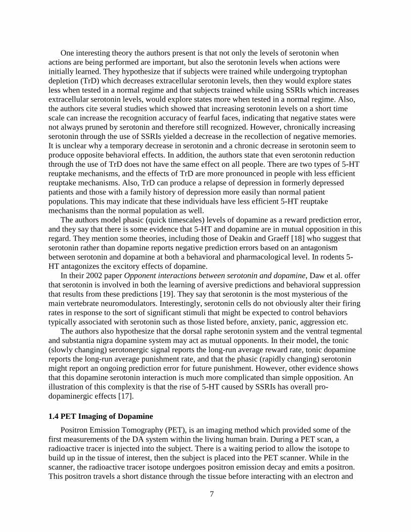
3.4.3 Multivariate Model ........................................................................................................... 29
3.4.4 Estimating 𝜷 Through Elastic Net Linear Regression ..................................................... 29
3.5 Using the Model to Make Predictions ................................................................................. 32
3.6 Failed Raman Spectroscopy Data Aquisition...................................................................... 32
3.6.1 Raman Spectroscopy Apparatus....................................................................................... 32
3.6.2 Raman Data Acquisition. ................................................................................................. 33
Chapter 4: Results ......................................................................................................................... 38
4.1 Cross Validation .................................................................................................................. 38
4.2 Univariate Model................................................................................................................. 38

v
Chapter 5: Conclusion................................................................................................................... 77
References ..................................................................................................................................... 79

vi
List of Figures Figure 1: Neurons Passing Messages to Each Other [4] ........................................................... 3
Figure 2: The Brain’s Dopamine Pathways [7] ........................................................................ 4
Figure 3: Comparison of Serotonin and Dopamine Pathways [12] .......................................... 6
Figure 4: Parts of a PET Scanner [21] ...................................................................................... 8
Figure 5: Dopamine Oxidation Peak in Fast-Scan Cyclic Voltammagram ............................ 17
Figure 6: Raman Spectroscopy Setup ..................................................................................... 18
Figure 7: The focus of this work was the wet lab data collection and making a predictive
model from flow cell CV data. ..................................................................................................... 20
Figure 8: Schematic of Flow Cell (Probe Tip Shown in Insert) ............................................. 21
Figure 9: Schematic of Headstage Amplifier.......................................................................... 22
Figure 10: Triangular Voltage Waveform .............................................................................. 22
Figure 11: Overlay of Applied Voltage Waveform, Raw Current Signal, and Derivative of
Signal for Varying Dopamine and Serotonin Levels .................................................................... 23
Figure 12: Images of wetlab probes (left) and the background charging current of each probe
(right). No dopamine or serotonin was present when the background charging current was
recorded......................................................................................................................................... 24
Figure 13: Overlay of all PBS waveforms over all trials (top) and standard deviation of
waveform at each time index over all trials (bottom). .................................................................. 25
Figure 14: Overlay of PBS waveforms from each probe for one trial (top) and standard
deviation of waveform at each time index for this trial (bottom). ................................................ 26
Figure 15: Total charge as a function of probe length (right) and sensitivity as a function of
probe length (left). The length of the shortest probe was normalized to 1. .................................. 27
Figure 16: Individual Contributions to the Generative Model................................................ 28
Figure 17: General Linear Model for Predictions ................................................................... 29
Figure 18: Applied Voltage, Measured Current, Derivative of Measured Current, and Beta
Vectors for Two Alpha Values ..................................................................................................... 31
Figure 19: Example Beta Vectors Overlaid on Voltammagram ............................................. 32
Figure 20: 100 mM Dopamine Spectra ................................................................................... 34
Figure 21: A Comparison of the Data from One Integration Period (Top), and Data Integrated
over 1000 of these Periods (Bottom) ............................................................................................ 35
Figure 22: Standard Deviation of Each Bin Showing Unequal Variances ............................. 36
Figure 23: An Example of an Artifact .................................................................................... 36
Figure 24: Standard Deviation of Bins after Artifact Removal .............................................. 37
Figure 25: Spectra of PBS after Artifact Correction ............................................................... 37
Figure 26: Probe 1 Predictions ................................................................................................ 39
Figure 27: Betas used for Probe 1 Predictions ........................................................................ 40
Figure 28: Increasing Serotonin Confusion Plot ..................................................................... 40
Figure 29: Increasing Dopamine Confusion Plot.................................................................... 41
Figure 30: Probe 2 Predictions ................................................................................................ 42
Figure 31: Betas used for Probe 2 Predictions ........................................................................ 42
Figure 32: Increasing Serotonin Confusion Plot ..................................................................... 43
Figure 33: Increasing Dopamine Confusion Plot.................................................................... 43
Figure 34: Probe 3 Predictions ................................................................................................ 44
Figure 35: Betas used to Predict Probe 3 ................................................................................ 44
Figure 36: Increasing Serotonin Confusion Plot ..................................................................... 45

vii
Figure 37: Increasing Dopamine Confusion Plot.................................................................... 45
Figure 38: Probe 4 Predictions ................................................................................................ 46
Figure 39: Betas used to Predict Probe 4 ................................................................................ 46
Figure 40: Increasing Serotonin Confusion Plot ..................................................................... 47
Figure 41: Increasing Dopamine Confusion Plot.................................................................... 47
Figure 42: Probe 5 Predictions ................................................................................................ 48
Figure 43: Betas used to Predict Probe 5 ................................................................................ 48
Figure 44: Increasing Serotonin Confusion Plot ..................................................................... 49
Figure 45: Increasing Dopamine Confusion Plot.................................................................... 49
Figure 46: Probe 1 Predictions ................................................................................................ 51
Figure 47: Betas used to Predict Probe 1 ................................................................................ 51
Figure 48: Increasing Serotonin Confusion Plot ..................................................................... 52
Figure 49: Increasing Dopamine Confusion Plot.................................................................... 52
Figure 50: Probe 2 Predictions ................................................................................................ 53
Figure 51: Betas used to Predict Probe 2 ................................................................................ 53
Figure 52: Increasing Serotonin Confusion Plot ..................................................................... 54
Figure 53: Increasing Dopamine Confusion Plot.................................................................... 54
Figure 54: Probe 3 predictions ................................................................................................ 55
Figure 55: Betas used to Predict Probe 3 ................................................................................ 55
Figure 56: Increasing Serotonin Confusion Plot ..................................................................... 56
Figure 57: Increasing Dopamine Confusion Plot.................................................................... 57
Figure 58: Probe 4 Predictions ................................................................................................ 58
Figure 59: Betas used to Predict Probe 4 ................................................................................ 58
Figure 60: Increasing Serotonin Confusion Plot ..................................................................... 59
Figure 61: Increasing Dopamine Confusion Plot.................................................................... 60
Figure 62: Probe 5 Predictions ................................................................................................ 61
Figure 63: Betas used to Predict Probe 5 ................................................................................ 61
Figure 64: Increasing Serotonin Confusion Plot ..................................................................... 62
Figure 65: Increasing Dopamine Confusion Plot.................................................................... 62
Figure 66: Comparison of Noise ............................................................................................. 63
Figure 67: RMS Error as Function of Percent of Beta Zeroed ............................................... 66
Figure 68: Components of Simulated Raman Spectra ............................................................ 67
Figure 69: Spectral Contribution of 1uM Dopamine .............................................................. 67
Figure 70: Spectral Contribution of 1uM Serotonin ............................................................... 68
Figure 71: 0.5uM Dopamine Spectra ...................................................................................... 69
Figure 72: 0.5uM Serotonin Spectra ....................................................................................... 69
Figure 73: 5uM Dopamine Spectra ......................................................................................... 69
Figure 74: 5uM Serotonin Spectra .......................................................................................... 70
Figure 75: 50uM Dopamine Spectra ....................................................................................... 70
Figure 76: 50uM Serotonin Spectra ........................................................................................ 70
Figure 77: Low Concentration Dopamine Beta ...................................................................... 71
Figure 78: Low Concentration Serotonin Beta ....................................................................... 71
Figure 79: Medium Concentration Dopamine Beta ................................................................ 72
Figure 80: Medium Concentraiton Serotonin Beta ................................................................. 72
Figure 81: High Concentration Dopamine Beta ..................................................................... 73
Figure 82: High Concentration Serotonin Beta ...................................................................... 73

viii
Figure 83: Low Concentration Dopamine Beta ...................................................................... 74
Figure 84: Low Concentration Serotonin Beta ....................................................................... 74
Figure 85: Medium Concentration Dopamine Beta ................................................................ 75
Figure 86: Medium Concentration Serotonin Beta ................................................................. 75
Figure 87: High Concentration Dopamine Beta ..................................................................... 75
Figure 88: High Concentration Serotonin Beta ...................................................................... 76
Figure 89: Correlation Coefficient vs. Concentration............................................................. 77

ix
List of Tables Table 1: Composition of Phosphate-Buffered Saline Solution ............................................... 21
Table 2: Raman Spectroscopy Data Collected ........................................................................ 34
Table 3: Summary of Univariate Model Performance ............................................................ 50
Table 4: Summary of Multivariate Model Performance ......................................................... 63
1
Chapter 1: Introduction In this chapter the motivation for this project will be explained, as well as an overview of the
research goals. Then some background on neurotransmitters, positron emission tomography,
functional magnetic resonance imaging, and animal models of Parkinson’s disease will be given.
1.1 Motivation
There are many functional neuroimaging techniques available to measure neural activity in
the brain. However, none of the existing methods are capable of measuring the release of
dopamine and serotonin in real time with good temporal resolution.
Electroencephalography (EEG) and magnetoencephalography (MEG) provide a way to
directly measure the activity of neurons by detecting either the electric or magnetic field that
results from current flowing through large populations of neurons. However, it is not possible to
accurately measure the firing activity of dopaminergic and serotonergic neurons because they are
so few in number and located deep enough in the brain that their activity is masked by other
overlying brain regions.
Positron emission tomography (PET) imaging and functional magnetic resonance imaging
(fMRI) imaging give an indirect measurement of neural activity by observing localized changes
in blood flow to different regions of the brain. In general, PET and fMRI have much better
spatial resolution than EEG and MEG (~1-2 mm), but much worse temporal resolution (~1 sec.
compared to 1 msec. for EEG and MEG). As opposed to EEG and MEG it is in fact possible to
measure dopamine and serotonin release with PET and fMRI through the use of contrast agents
which bind to these chemicals. However, the time resolution for these methods is very poor, on
the order of 10s of seconds.
Fast-scan cyclic voltammetry (FSCV) is unique in that it provides a way to measure the
concentration of dopamine and serotonin in the extracellular space with sub second time
resolution. Prior to 2011 [1] FSCV had never been reported in humans because it requires a
probe to be placed into the neural tissue where the concentration measurements are made.
Recently however, neurosurgeons have placed fast-scan cyclic voltammetry probes into the
striatum of human patients who were undergoing deep brain stimulation (DBS) electrode
implantation surgery. These measurements are the first of their kind, and potentially allow the
concentration of dopamine and serotonin in the extracellular space to be measured with a time
resolution of 100 ms. Because many of the patients from which the data was recorded have
Parkinson’s disease, this data has the potential to provide a better understanding of this disease
which involves the death of dopaminergic neurons. However, it also has the potential to provide
insight to the function of these chemicals in a healthy human brain. Fast-scan cyclic voltammetry
(FSCV) does have some drawbacks. It is extremely invasive when compared to PET or fMRI,
and the probe relies on chemical reactions with the surrounding cortical tissue meaning that it
can only be used temporarily. Also, it requires advanced signal processing techniques to extract
useful concentration information from the data and differentiate between different
neurotransmitters.
Raman spectroscopy is a possible alternative to FSCV that uses light to make chemical
measurements. The main advantage of this technique is that a probe using Raman spectroscopy
could be permanently implanted into a patient’s brain and allow measurement of
neurotransmitter concentrations over a long period of time. The ability to continuously monitor

2
neurotransmitter release in the brain could be a huge asset to doctors trying to treat neurological
disorders, for example to better assess drug dose requirements. Also, Raman spectroscopy has
the potential to offer much better differentiation between types of neurotransmitters than FSCV
and also allow the detection of chemicals that aren’t electrically active. This is because Raman
spectroscopy probes the vibrational frequencies of a molecule directly using light.
1.2 Project Overview
As mentioned above, the research presented here was motivated by fast-scan cyclic
voltammetry data collected in the striatum of human patients undergoing DBS surgery at Wake
Forest University [1]. A prerequisite to testing for neurotransmitter levels in these data was to
develop a signal processing method that could be validated in known settings. Thus the aim of
my research was to develop a model which could take the recorded cyclic voltammagram as an
input, and output the molar concentration of dopamine and serotonin that was present at the tip
of the probe when the voltammagram was recorded. This is not at all a simple process, and much
work has already been done on ways to accurately make this conversion.
For our solution to this problem, prepared concentrations of dopamine and serotonin were
first prepared in the lab and cyclic voltammetry data was recorded from a probe placed in a flow
cell. This data was used to make models that allow the voltammetry data collected from the
patients to be converted to concentrations of dopamine and serotonin. Data was collected on 5
probes, and this data was used to make several models and compare the accuracy of each model.
Once a suitable model was chosen, it was used to make predictions on the patient data.
Raman spectroscopy data was also collected in a lab at Virginia Tech using prepared
concentrations of dopamine to study the feasibility of replacing the FSCV probe with a Raman
spectroscopy probe. Simulated Raman spectroscopy data was also generated and used to show
how the elastic net algorithm could be applied to data this type of data.
1.3 What are neurotransmitters? Why are they important?
Neurons (also known as nerve cells) are responsible for processing and transmitting
information in the brain through the use of electrical and chemical signaling. One of the most
important properties of neurons and what makes them different from most other cells in the body
is that they can “fire”, or create an electrochemical pulse known as an action potential. This pulse
quickly travels down the long neuron projection known as the axon, and can cause nearby
neurons to fire as well. In this way information is passed from one neuron to the next through the
central nervous system (CNS). Interestingly, heart cells are also capable of firing and creating
action potentials as do neurons in the CNS. The rhythmic activity of the heart results from the
discharge of excitatory impulses by cells in a region of the heart known as the sinoatrial node.
These cells automatically fire in a regular pattern that results from each action potential being
followed by a slow depolarization that brings the membrane to its threshold potential, thereby
evoking another action potential in a repeating cycle [2].
The fastest rate at which neurons can fire is approximately 200Hz with most firing at much
lower rates than this. Dopamine neuron (a specific type of neuron which this work focuses on)
firing rates in mice have been observed to range from 0.8-12.7 Hz, with a mean firing rate of 4.6
Hz [3]. A typical neuron located in the cerebral cortex (the outer layer of brain tissue) receives
input from a few thousand upstream neurons and passes on messages to a few thousand
downstream neurons. In one cubic millimeter of cortical tissue, there are approximately one

3
hundred thousand neurons. This adds up to a total of approximately 40 billion neurons in the
average human cortex, each with thousands of connections to other neurons. Below in Figure 1 is
a diagram of two neurons in which the neuron on the left is firing and passing a message
downstream to the neuron on the right.
Figure 1: Neurons Passing Messages to Each Other [4]
The connections between individual neurons are called synapses. These synapses are
classified according to the type of cellular structures which make up the presynaptic and
postsynaptic components. In Figure 1 the neuron on the upper right is the presynaptic neuron
because it sends information to the postsynaptic neuron on the lower left. The most common
synapses in the human brain and the type of synapse depicted in Figure 1 are axo-dendritic
synapses where the axon of the presynaptic neuron terminates on the dendrites of the
postsynaptic neuron. In other synapses found in the brain, the axon of the presynaptic cell may
synapse onto a cell body, another axon, into the bloodstream, or diffusely into the adjacent
nervous tissue.
The chemicals used by neurons to send messages across synapses to other neurons are known
as neurotransmitters. Neurotransmitters are stored inside of a neuron in containers known as
synaptic vesicles. When the membrane potential of the neuron exceeds a particular threshold
value of -40 mV, the neuron fires and generates a millisecond long pulse called an action
potential. When an action potential occurs in a neuron, some of the synaptic vesicles containing a

4
neurotransmitter move to the presynaptic membrane of the neuron and release their contents the
synaptic cleft (the space between the two cells). Once released into the synapse, these
neurotransmitters can attach to receptors located in the cell membrane of the postsynaptic cell.
The attaching or “binding” of neurotransmitters to the receptors can either make the postsynaptic
cells more likely to fire (known as an excitatory effect) or less likely to fire (known as an
inhibitory effect) depending on the type of neurotransmitter and the type of receptor it binds to.
This is because particular receptors admit charged particles into the cell, such as chloride (a
negative ion) or sodium (a positive ion). Receptor binding can also lead to indirect effects on
postsynaptic depolarization via protein cascades within the cell. Over 100 types of
neurotransmitters have been discovered, though most of the compounds which function as
neurotransmitters can be divided into three main chemical families: amines (a group of
molecules containing molecules of carbon, hydrogen, and nitrogen), amino acids (organic
compounds containing both an amino group and a carboxylic acid group), and peptides
(compounds which are made up of multiple amino acids) [5].
Dopamine (DA) is the neurotransmitter which will be the main focus of this paper.
Dopamine is a neurotransmitter in the amine family (the DA molecule is called a monoamine
because it contains only one amine group) and is produced by a group of neurons referred to as
dopaminergic neurons. There are only approximately 400,000 of these neurons in the human
brain [6], and their cell bodies are concentrated in only a few locations. The two main sites of
dopaminergic neuron cell bodies are the substantia nigra (SN) and the ventral tegmental area
(VTA). The axons of these dopaminergic neurons extend to many other parts of the brain where
they can release dopamine into the extracellular space. A large number of these dopaminergic
neurons terminate in the striatum, a region of the brain, where the measurements from patients
were recorded.
Figure 2: The Brain’s Dopamine Pathways [7]
The death of dopaminergic neurons in the substantia nigra is responsible for the debilitating
motor impairment associated with Parkinson’s disease. Parkinsonian symptoms do not occur
until 50%-80% of the dopaminergic neurons in the substantia nigra have died, and it is not clear
what causes the death of these neurons in Parkinson’s disease. These neurons can also be
destroyed by neurotoxins and viral infections such as encephalitis lethargica, resulting in similar
movement disorders to those seen in Parkinson’s disease.
The basal ganglia comprise several subcortical nuclei or clusters of densely packed neuron
cell bodies. It is composed of parts of the brain including the dorsal striatum (caudate nucleus

5
and putamen), ventral striatum (nucleus accumbens and olfactory tubercle), globus pallidus,
ventral pallidum, substantia nigra, and subthalamic nucleus. The leading model of basal ganglia
function states that two circuits, the direct and indirect pathways, originate from two distinct
populations of striatal medium spiny neurons (MSNs) and project to different output structures.
Activity in the direct pathway MSNs is believed to promote movement, while activity in the
indirect pathway MSNs is believed to inhibit it. The direct and indirect pathways are
characterized by their different expression of dopamine receptors. D1 (the different types of
receptors are identified by a subscript) DA receptors stimulate GABAergic neurons in the
presence of DA and are expressed by direct pathway MSNs whereas D2 receptors inhibit
GABAergic neurons in the presence of dopamine and are expressed by indirect pathway MSNs
[8].
More is known about the function of dopamine in the CNS than most any other
neurotransmitter, in particular its algorithmic or computational role. However, its exact function
is still far from certain. Schultz et al. hypothesized in their 1997 paper titled A Neural Substrate
of Prediction and Reward, that dopamine’s role is to signal changes or errors in the predictions
of future salient and rewarding events [9]. These changes or errors in the prediction of future
salient and rewarding events are called reward predictions errors. According to their paper, it has
long been known that dopaminergic neurons in the VTA and SN are involved with the
processing of rewarding stimuli. Some of the evidence to support this theory is that drugs like
amphetamine and cocaine are addictive because they can bind to dopamine receptors – i.e. they
mimic dopamine at exaggerated levels [10]. Also, mice will choose to press bars to excite
dopamine neurons at the site of an electrode over other rewarding activities including food and
sex. If animals are treated with dopamine receptor blockers, they learn less rapidly to press a bar
for a reward food pellet.
The reward prediction error which the authors hypothesize is encoded by dopamine is
delivered to various structures throughout the brain and used by them to influence the processing
of predictions and to guide choice toward reward-maximizing actions. They hypothesize that in
the striatum, the reward prediction error, also known as a scalar prediction signal, could have a
direct effect on the choice of action to take. One reason they believe this is that in the striatum,
activity relating to conditioned stimuli has been observed in several studies. The dopamine signal
in the striatum is believed to encode the reward prediction error and may influence behavioral
choices by modulating the level of competition of motor plans in the dorsal striatum. There is
evidence for the striatal plasticity, or the ability of synapse connections to strengthen or weaken
over time, after pulsatile application of dopamine. They also state that it seems reasonable to
require that the prediction errors be delivered to the regions most responsible for making the
predictions. This means that it is expected that there is a mechanism to couple local activity in
the cortex to an enhanced sensitivity of nearby dopamine terminals to differences from baseline
spike production along the parent axon. Lastly, this paper makes the point that neuromodulatory
systems such as the dopamine system were so named because it was believed that they work with
slower time resolution than do other connections in the brain like glutamatergic connections.
While this may be true in part, this paper shows that neuromodulatory systems may also deliver
precisely timed information to specific target structures.
A second important neurotransmitter which my research focuses on is Serotonin (5-HT).
Serotonin is similar to dopamine in that it is a monoamine neurotransmitter and the cell bodies of
the cells which produce serotonin are only located in a few specific locations in the brain.
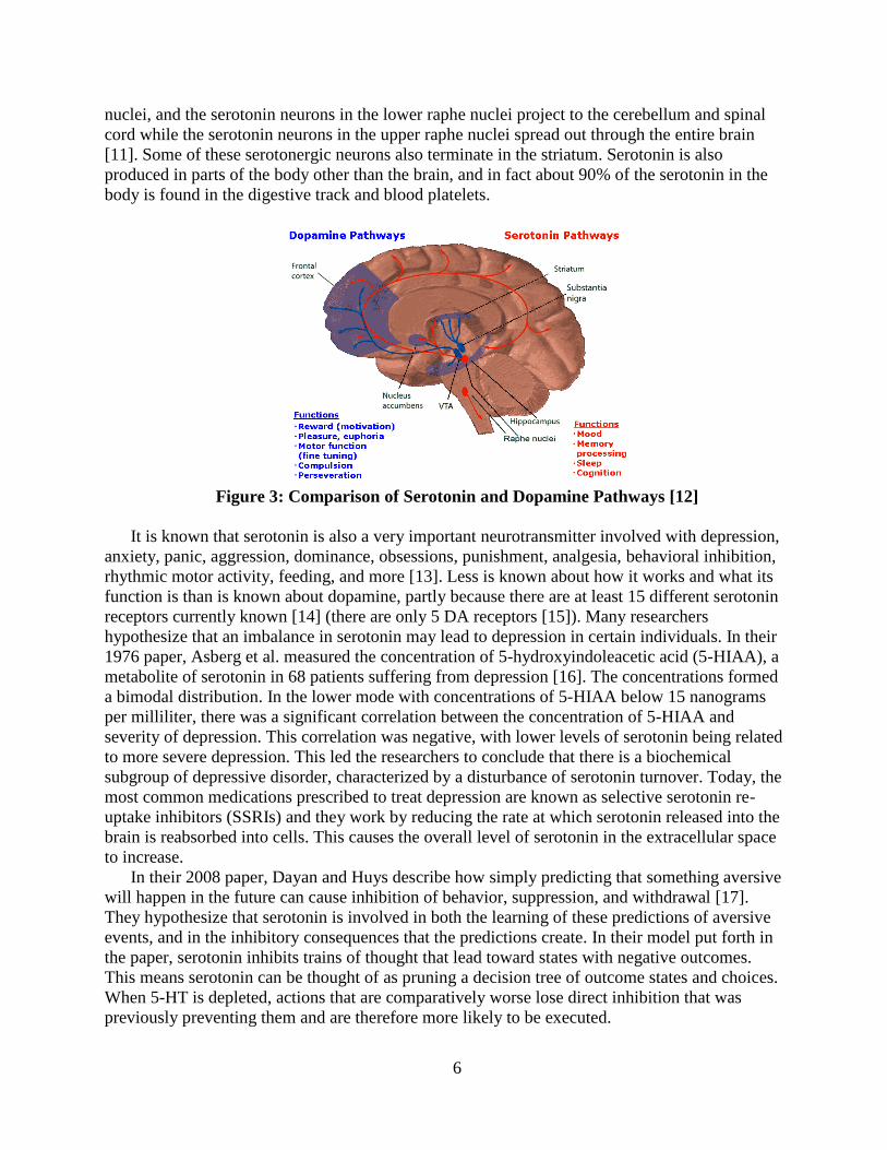
Serotonin is produced primarily by neurons in the raphe nuclei. There are 7 to 8 of these raphe
6
nuclei, and the serotonin neurons in the lower raphe nuclei project to the cerebellum and spinal
cord while the serotonin neurons in the upper raphe nuclei spread out through the entire brain
[11]. Some of these serotonergic neurons also terminate in the striatum. Serotonin is also
produced in parts of the body other than the brain, and in fact about 90% of the serotonin in the
body is found in the digestive track and blood platelets.
Figure 3: Comparison of Serotonin and Dopamine Pathways [12]
It is known that serotonin is also a very important neurotransmitter involved with depression,
anxiety, panic, aggression, dominance, obsessions, punishment, analgesia, behavioral inhibition,
rhythmic motor activity, feeding, and more [13]. Less is known about how it works and what its
function is than is known about dopamine, partly because there are at least 15 different serotonin
receptors currently known [14] (there are only 5 DA receptors [15]). Many researchers
hypothesize that an imbalance in serotonin may lead to depression in certain individuals. In their
1976 paper, Asberg et al. measured the concentration of 5-hydroxyindoleacetic acid (5-HIAA), a
metabolite of serotonin in 68 patients suffering from depression [16]. The concentrations formed
a bimodal distribution. In the lower mode with concentrations of 5-HIAA below 15 nanograms
per milliliter, there was a significant correlation between the concentration of 5-HIAA and
severity of depression. This correlation was negative, with lower levels of serotonin being related
to more severe depression. This led the researchers to conclude that there is a biochemical
subgroup of depressive disorder, characterized by a disturbance of serotonin turnover. Today, the
most common medications prescribed to treat depression are known as selective serotonin re-
uptake inhibitors (SSRIs) and they work by reducing the rate at which serotonin released into the
brain is reabsorbed into cells. This causes the overall level of serotonin in the extracellular space
to increase.
In their 2008 paper, Dayan and Huys describe how simply predicting that something aversive
will happen in the future can cause inhibition of behavior, suppression, and withdrawal [17].
They hypothesize that serotonin is involved in both the learning of these predictions of aversive
events, and in the inhibitory consequences that the predictions create. In their model put forth in
the paper, serotonin inhibits trains of thought that lead toward states with negative outcomes.
This means serotonin can be thought of as pruning a decision tree of outcome states and choices.
When 5-HT is depleted, actions that are comparatively worse lose direct inhibition that was
previously preventing them and are therefore more likely to be executed.
7
One interesting theory the authors present is that not only the levels of serotonin when
actions are being performed are important, but also the serotonin levels when actions were
initially learned. They hypothesize that if subjects were trained while undergoing tryptophan
depletion (TrD) which decreases extracellular serotonin levels, then they would explore states
less when tested in a normal regime and that subjects trained while using SSRIs which increases
extracellular serotonin levels, would explore states more when tested in a normal regime. Also,
the authors cite several studies which showed that increasing serotonin levels on a short time
scale can increase the recognition accuracy of fearful faces, indicating that negative states were
not always pruned by serotonin and therefore still recognized. However, chronically increasing
serotonin through the use of SSRIs yielded a decrease in the recollection of negative memories.
It is unclear why a temporary decrease in serotonin and a chronic decrease in serotonin seem to
produce opposite behavioral effects. In addition, the authors state that even serotonin reduction
through the use of TrD does not have the same effect on all people. There are two types of 5-HT
reuptake mechanisms, and the effects of TrD are more pronounced in people with less efficient
reuptake mechanisms. Also, TrD can produce a relapse of depression in formerly depressed
patients and those with a family history of depression more easily than normal patient
populations. This may indicate that these individuals have less efficient 5-HT reuptake
mechanisms than the normal population as well.
The authors model phasic (quick timescales) levels of dopamine as a reward prediction error,
and they say that there is some evidence that 5-HT and dopamine are in mutual opposition in this
regard. They mention some theories, including those of Deakin and Graeff [18] who suggest that
serotonin rather than dopamine reports negative prediction errors based on an antagonism
between serotonin and dopamine at both a behavioral and pharmacological level. In rodents 5-
HT antagonizes the excitory effects of dopamine.
In their 2002 paper Opponent interactions between serotonin and dopamine, Daw et al. offer
that serotonin is involved in both the learning of aversive predictions and behavioral suppression
that results from these predictions [19]. They say that serotonin is the most mysterious of the
main vertebrate neuromodulators. Interestingly, serotonin cells do not obviously alter their firing
rates in response to the sort of significant stimuli that might be expected to control behaviors
typically associated with serotonin such as those listed before, anxiety, panic, aggression etc.
The authors also hypothesize that the dorsal raphe serotonin system and the ventral tegmental
and substantia nigra dopamine system may act as mutual opponents. In their model, the tonic
(slowly changing) serotonergic signal reports the long-run average reward rate, tonic dopamine
reports the long-run average punishment rate, and that the phasic (rapidly changing) serotonin
might report an ongoing prediction error for future punishment. However, other evidence shows
that this dopamine serotonin interaction is much more complicated than simple opposition. An
illustration of this complexity is that the rise of 5-HT caused by SSRIs has overall pro-
dopaminergic effects [17].
1.4 PET Imaging of Dopamine
Positron Emission Tomography (PET), is an imaging method which provided some of the
first measurements of the DA system within the living human brain. During a PET scan, a
radioactive tracer is injected into the subject. There is a waiting period to allow the isotope to
build up in the tissue of interest, then the subject is placed into the PET scanner. While in the
scanner, the radioactive tracer isotope undergoes positron emission decay and emits a positron.
This positron travels a short distance through the tissue before interacting with an electron and

8
being annihilated. This positron-electron interaction creates a pair of gamma photons. Since each
photon created has nonzero momentum, conservation of momentum means that they must travel
in opposite directions. Detectors placed around the perimeter of the PET scanner detect these two
photons as they strike the detector ring almost simultaneously [20].
Figure 4: Parts of a PET Scanner [21]
When a pair of photons interact with the ring of detectors it can be inferred that the location
of the positron-electron interaction lies on the line between the detector pairs as shown in Figure
4. Using image reconstruction algorithms, the concentration of the radioactive isotope in each
voxel can be computed resulting in a 3D concentration map. To recap, first some type of
molecule tagged with a radioactive tracer is injected into the body. After allowing enough time
for the tracer to disperse through the body, a PET scan allows a 3D map of where the molecule
ended up to be generated.
The PET measurements of the DA system are indirect, and rely on the use of radiotracers to
label molecules such as DA receptors, DA transporters, and DA precursors. A ligand is a
substance that forms a complex with a biological molecule, an example of a specific type of
ligand is a neurotransmitter such as dopamine which binds to a receptor. In PET imaging, ligands
are often radiolabeled with a radioactive isotope. Raclopride is a ligand that can be labeled with a
radioactive carbon-11 atom and is often used in PET imaging because it binds to some types of
dopamine receptors. Once ligands are radiolabeled they are then injected into the tissue under
study and bind with their corresponding receptor. In PET imaging, often the ligand-receptor
binding kinetic properties are measured, but presynaptic dopamine turnover can be measured as
well. Unfortunately, PET scans are slow and can require up to two hours to complete. PET can
also require the sampling of arterial blood for molecular studies, which is mildly invasive and
painful.
As an example of how PET imaging and labeled ligands can be used to study the
dopaminergic system, Cicchetti et al. administered a chemical known as 6-OHDA to rats and
monitored the degradation of dopaminergic neurons using PET imaging of presynaptic dopamine
transporters [22]. 6-OHDA is a neurotoxin that causes dopaminergic cells in the substantia nigra

9
to die. The results of 6-OHDA lesioning are symptoms that closely resemble those of
Parkinson’s disease. The specific ligand used in this study to bind to dopamine transporters was
[11C]-CFT. The [11C] at the beginning of the name means that carbon-11 is the radioactive
isotope used to tag the CFT molecule. CFT is a dopamine reuptake inhibitor that is an analog of
cocaine and easily binds to dopamine transporters. Their study revealed a significant decrease in
the binding parameters of [11C]-CFT in the striatum after 6-OHDA lesioning. The [11C]-
PK11195 ligand was also administered in parallel to measure the inflammatory response of the
brain. The [11C]-PK11195 ligand attaches to activated microglia, cells whose job it is to provide
immune defense in the central nervous system. This ligand allowed them to determine that
inflammation is a significant component of progressive dopaminergic degeneration that can be
monitored by PET imaging.
A recent article by Le Foll et al. [23] also shows how PET imaging can be used to monitor
the occupancy of two different types of dopamine receptors in the same experiment. They test
the drug buspirone to see how well it binds to D3 receptors compared with D2 receptors with
hopes that it could be used to treat drug addiction. Previous findings suggested that buspirone
binds to D3 receptors much more readily than it does to D2 receptors and also that it disrupts
psychostimulant self-administration in preclinical models. D3 receptors were chosen as targets
for drug addiction treatment because preclinical and post-mortem human brain studies have
found that D3 receptor levels are elevated after chronic exposure to drugs of abuse and also PET
data has shown D3 receptor levels to be higher in individuals who abuse stimulants. A labeled
ligand of [11C]-(+)-PHNO was used to test whether the buspirone binds to D3 receptors more
than D2 receptors. Amounts of [11C]-(+)-PHNO binding in the dorsal striatum reflect D2 receptor
availability while in other regions including the hypothalamus and substantia nigra it reflects D3
receptor availability. Their hypothesis was that buspirone did more readily bind to D3 receptors,
and therefore a selective decrease in [11C]-(+)-PHNO binding in D3 rich areas relative to D2 areas
would be observed. Magnetic Resonance (MR) structural images were also acquired to aid
region of interest delineation of the PET images. The cerebral cortex was used as a reference
region for the PET images. These previous two studies give indications as to how PET imaging
can and has been used to study the body’s dopamine system. In the first study, the labeled ligand
bound itself to a dopamine transporter protein and another labeled ligand used bound itself to
activated microglia cells. In the second study, the labeled ligand used bound itself to D2 and D3
dopamine receptors.
The most common protein classes studied with PET are neuroreceptors, ligand transporters,
and enzymes. PET currently works best when changes in protein density are very large (>50%).
Some radiotracers are sensitive to the receptor occupancy while others are not. As an example,
there are several sensors for the 5-HT system which appear to be insensitive to the amount of
endogenous 5-HT being released. This has been tested by administering drugs that alter serotonin
levels in the brain and seeing that these sensors do not show a change in receptor density. In
general, before a PET signal change can be attributed to a protein density change it is necessary
to perform additional testing to ensure that the binding of the radiotracer to the protein is not
affected by other chemicals or neurotransmitters that can also bind to the protein and compete
with the radiotracer.
Despite the success of PET imaging with dopamine, only a few other neuroreceptor systems
have demonstrated success in measuring endogenous fluctuations. There is a need to design a
new generation of radiotracers with faster protein association. This could allow multiple releases
of neurotransmitters with a high time resolution to be monitored. Current imaging-tracer

10
techniques only allow for detection of a single neurochemical release over a relatively long
period of time. These studies mentioned in this section show the great variety of measurements
that are possible to make with PET imaging. The main drawback to PET imaging however is the
time required to take a scan. PET imaging can be used to monitor changes in the dopamine
system that take place over the course of several minutes or hours, but monitoring phasic
dopamine levels over the course of seconds or even fractions of second is not currently possible.
1.5 fMRI Imaging of Dopamine
Magnetic Resonance Imaging (MRI) is another type of imaging modality similar in some
ways to PET imaging. However instead of using radiolabeled molecules and radiation detectors
as does PET, MRI relies on large magnetic fields to partially polarize the nuclear spins of atoms
within a patient. The spins are then excited with a properly tuned pulse of radio frequency
radiation. When the atoms relax from this radio frequency (RF) excitation, they emit a small
amount of radio frequency information which can be detected and used to infer the structure of
the cross section of tissue present. This allows brain anatomy to be studied non-invasively in
great detail.
Approximately 20 years ago it was discovered that MRI imaging could be made sensitive to
brain activity as well as brain anatomy. The magnetic resonance (MR) signal is not sensitive
directly to neuronal activity, but can detect changes in blood flow which occur as an indirect
result of neural activity [24]. When neuronal activity in a particular part of the brain increases,
the body sends an oversupply of oxygenated blood to that area. This causes the oxygen level of
blood in the region surrounding the neuronal activity to increase, a change that can be detected
by the MRI machine because oxygenated hemoglobin and deoxygenated hemoglobin have
different magnetic signatures. This process of imaging neuronal activity based on blood flow is
called functional MR imaging (fMRI) and the signal it detects is called the blood oxygenation
level dependent (BOLD) signal. The hemodynamic response imaged by BOLD signals begin
approximately two seconds after neural stimulation and peak after four to six seconds. Also, the
hemodynamic response is thought to encode the total cellular activity within a region rather than
single cell activity. The BOLD signal is believed to represent the local field potential during
neural stimulation [25].
It is possible to image brain structures in the dopamine system such as the subthalamic
nucleus (STN) and the substantia nigra (SN) using the BOLD signal and fMRI, but there are
many limitations to doing this [26]. These structures are very small, and their location can vary
considerably from one person to the next. Their size is less than the spatial resolution of most
fMRI scanning sequences. Hollander et. al. show that fMRI signals reported in previous studies
of these structures are likely a mixture of signals from the STN, SN, and the surrounding tissue
instead of resulting from only one structure. They recommend that the standard smoothing
strategies used for fMRI imaging should be avoided altogether when trying to study the activity
of small subcortical nuclei. They further recommend that individual anatomical masks should be
used based on a structural scan of the individual.
In the article Detection of dopaminergic neurotransmitter activity using pharmacological
MRI: correlation with PET, Microdialysis, and Behavioral Data [27] the use of fMRI to measure
dopamine neurotransmitter activity was investigated. The dopamine system has high regional
specificity, unlike the glutamatergic system, with most of the receptors being located in the
frontal cortex and basal ganglia. Also, the dopamine system in animals can be selectively

11
destroyed using 6-hydroxydopmine. This allows it to be determined if the fMRI response
measured in this experiment is due to dopamine.
Rats were used for this study, with microdialysis probes placed into the striatum of the rats.
Control and lesioned rats were used, with 6-OHDA injected to kill at least 90% of the
dopaminergic neurons in the lesioned rats. All MR measurements were performed in a 4.7T GE
Omega CSI imager.
Either the drug D-amphetamine or CFT was injected intravenously while fMRI images where
acquired or 90-180 minutes post injection. In these fMRI experiments the hemodynamic
response being measured is caused by drug administration rather than task dependent activation
and are therefore termed pharmacological MRI (phMRI) experiments. PET measurements were
also acquired on the same animals after being scanned by phMRI. Dopamine transporters were
imaged using carbon-11 labeled CFT as a tracer.
Their results showed that both amphetamine and CFT administration cause an increase in
BOLD signal activity observed through phMRI imaging. Furthermore, these signal increases
were localized to regions of the mouse brain known to be high in dopaminergic receptor density.
The authors admit that there are some potential problems with such an experiment, mainly
because the metabolic response to the neurotransmitter binding rather than the binding itself is
being observed by the phMRI, whereas in PET imaging, the actual binding of the ligand (in this
case CFT) to the receptor is what is being observed. Also, for phMRI experiments, a large dose
of the drug is necessary, and in the case of amphitamines, such large doses have the potential to
activate other monoamine neurotransmitter systems such as serotonin. This means that the
response seen may not be only a function of dopamine. Lastly, if the phMRI hemodynamic
response is only indirectly coupled to the neurotransmitter release, then the signal observed may
not provide useful information about the actual neurotransmitter release.
It was also observed that the BOLD response on the ipsilateral side of the brain was greatly
diminished for those that underwent 6-OHDA administration. It is clear that this response was
due to endogenous dopamine because Gd-DTPA (a MRI contrast agent used to map out blood
flow) administration revealed that there was no change in relative cerebral blood volume (rCVB)
or relative cerebral blood flow (rCBF). This means that the 6-OHDA only affected the dopamine
system and not the vascularization or the hemodynamics on the side that was lesioned. The
degeneration of the dopamine system on the ipsilateral side could also be seen by using [11C]-
labeled CFT and PET imaging. They conclude that the phMRI response observed was due to
release of dopamine in the striatum.
Parkinson’s disease doesn’t occur until approximately 80% of the dopaminergic neurons die.
This means it may be possible to use phMRI (MRI along with administration of CFT) as a
prescreening for the early stages of Parkinson’s disease. The authors do mention that it is still
unclear if the metabolic response is due to the presynaptic uptake of dopamine or the
postsynaptic stimulation of D1 and D2 receptors.
In their 2010 paper Mikhail Shapiro [28] introduced the development of a MRI contrast agent
for imaging dopamine which could someday be used in humans for Parkinson’s disease
diagnosis. This method would work differently from the phMRI technique previously mentioned
in which the BOLD response to a drug such as CFT is monitored. Instead of imaging the
changing magnetic properties of the blood in the brain, the magnetic properties of the contrast
agent itself are what is imaged. The researchers state that MRI is capable in ideal circumstances
of providing information at high spatial (<100 um) and temporal (~1s) resolutions from living
specimens. BOLD imaging is based on hemoglobin, and this can be thought of as endogenous

12
oxygen-sensitive MRI contrast agent present in blood. However, this provides only a slow and
indirect readout of neural activity because of the complexity of neurovascular coupling. They
worked to developed a dopamine sensitive MRI contrast agent by modifying the bacterial
cytochrome P450-BM3 (BM3). A cytochrome is an iron containing protein. When a ligand binds
to a particular site on this protein, it leads to a drop in the MRI signal enhancement. However, as
the protein naturally occurs, dopamine does not easily bind to its receptor site. To make the
protein able to bind to dopamine, the researchers used an absorbance-based screen and a
technique known as directed evolution to shift the specificity of BM3 away from its natural
ligand and towards dopamine. Directed evolution is a molecular engineering method that uses
rounds of mutation and selection to generate proteins with novel functionality. This approach of
modifying proteins through directed evolution could be generalized to create probes for other
targets besides dopamine. After creation of the DA sensitive BM3 sensor, it was injected into the
brain of living rats. Then to test for the ability to measure endogenous DA a solution with
elevated K+ levels was injected as K+ is known to release large amounts of DA into the striatum.
The DA sensitive BM3 was injected into one hemisphere and the unmodified BM3 was injected
into the other to ensure that the observed MR signal changes were only due to dopamine. The K+
injections produced a discernable signal decrease of up to 3% near the DA sensitive BM3
injection site. B
The researchers believe that these contrast agents will allow functional neuroimaging
based on direct detection of neuronal events rather than hemodynamic changes. Also, exogenous
delivery of macromolecules such as BM3 to large regions of animal brains should be possible,
possibly through the use of transgenic subjects. Because of their small size, BM3-based DA
sensors might sample synaptic dopamine better than voltammetry or microdialysis probes. With
appropriate targeting it could become synapse specific and offer a combination of spatial
coverage and precision that is currently inaccessible to other methods and potentially well suited
to the types of studies of dopaminergic function that we are interested in.
Another way to indirectly assess dopamine and serotonin in fMRI is by using tasks
known to elicit signals in their respective nuclei. This is currently most appropriate for dopamine
since its computational correlates are well documented. For example in the article Testing the
Reward Prediction Error Hypothesis with an Axiomatic Model [29], rewards were defined as
stimuli that elicit approach behaviors, include subjective feelings of pleasure during
consumption, and lead to reinforcement of cues and actions. There are a variety of brain
structures both cortical and subcortical which make up the brain’s reward circuit, but the striatum
lies at the core of these circuits. Many fMRI experiments have attempted to understand how the
striatum contributes to reward processing. In this article, an approach known as the axiomatic
approach which is rooted in economic theory is used to formally test the entire class of RPE
models on neural data. They show that fMRI measurements of the striatum, medial prefontal
cortex, amygdala, and posterior cingulate cortex satisfy necessary and sufficient conditions for
the entire class of RPE models. The authors state that although parameterized temporal
difference approaches have been shown to account for electrophysiological data very well,
regression approaches cannot in principle falsify they hypothesis that dopamine-related activity
encodes some kind of RPE signal and therefore cannot formally test this hypothesis. Caplin and
Dean [30] recently examined the necessary and sufficient properties of any RPE signal. They
showed that any RPE signal must possess three critical features. The authors then devised an
fMRI experiment where the BOLD response was measured in subjects’ brains as they played

13
monetary lotteries for real money. Subjects played a lottery with two prizes available +$5 and -
$5 at a variety of probabilities 0-100% in 25% increments.
They performed two analyses. First, they used the traditional regression-based analysis.
This required that several assumptions about reward and expectation were made. They assumed
that reward is a linear function of monetary reward with no change in slope at the origin. They
also assumed that predicted reward was equal to the utilities of the prized weighted by their
objective probabilities. This requires that the RPE signal is then proportional to the difference in
dollars between the outcome received and the lottery’s expected value. They also had to
hypothesize that the BOLD response would follow the canonical two-gamma hemodynamic
impulse response function. With these parameterizations, they found that BOLD activity in the
striatum (including the nucleus accumbens, putamen, and caudate) was significantly correlated
with RPE at the p<0.001 uncorrected level. At p<0.01 BOLD activity in the medial prefrontal
cortex was also correlated with the RPE term. However, other candidate areas were not
correlated significantly including the anterior insula, amygdala, and posterior cingulate cortex.
According to the authors, this correlation cannot however tell us whether or not the data are
compatible with the RPE hypothesis. It is impossible to tell from this data analysis whether the
reason no significant correlation is observed was because of a fundamental mismatch between
the actual signal and the model, or if our current measurements are simply not sensitive enough
to tell. They further state that plotting the average BOLD response to positive and negative
outcomes from the three two-prize lotteries showed that the hemodynamic responses to outcomes
in the amygdala, posterior cingulate cortex, and also the medial prefrontal cortex do not at all
resemble the canonical hemodynamic response.
The axiomatic approach used was fairly unique because it required no assumptions about
the nature of the unobservable subjective variables like reward and expectation. Instead of
looking for correlations with specific RPE models, it tests approaches critical to the entire RPE
model class. They showed that BOLD activity in the anterior insula falsifies the axiomatic model
for RPE and therefore cannot encode RPEs. However, the anterior insula almost completely
satisfied an alternate model for RPE absolute value or salience. There are several theories which
suppose dopamine neurons and dopamine-related activity may encode salience in addition to or
instead of RPEs. A recent electrophysiological study found neurons in the dorsolateral substantia
nigra that increase activity in response to both unexpected appetitive and aversive events.
A disadvantage of the axiomatic approach is that regions of interest must be specified
manually by the experimenter. With regression-based methods, candidate RPE areas can be
identified through a whole brain analysis. They state that future research could establish whether
the quantity of dopamine release in these areas measured with electrochemical methods satisfies
the axiomatic model, directly testing the linkage between RPE representations and dopamine.
Given the still to be determined function of serotonin this approach has not been attempted to
identify serotonergic modulation of cortical regions.
1.6 Animal models of PD & dopamine dysfunction
Models of neurotransmitter dysfunction present in cases of pathology offer insights into the
normative roles of neurotransmitters. In turn models of neurotransmitter pathology can be used
to mimic the human condition. These models can either be in vitro or in vivo. In vitro models
(meaning in glass tubes) are performed outside of a living organism. As research progresses in
vivo (meaning in living animals) models are eventually used. This means that it is necessary to
have a way of reproducing the disease, in this case Parkinson’s, in a living animal.

14
In their article Animal Models of Parkinson’s Disease, Fabio Blandini and Marie-Therese
Armentero [31] describe some of the more common animal models used to study Parkinson’s
disease. Parkinson’s disease is characterized by the death of dopaminergic neurons in the
substantia nigra, therefore animal models of the disease must somehow kill the dopaminergic
neurons in these locations. The first PD animal models developed relied on using
pharmacological agents which selectively kill dopaminergic neurons in the substantia nigra.
There are several agents currently in use, each with their own benefits and drawbacks. There is
no perfect agent which creates an exact model of PD, but different agents are able to recreate
different aspects of the disease.
Pharmacological agents can be broadly divided into two categories, those which are
systemically administered, meaning that they do not need to be injected directly into the animal’s
brain, and those that are locally administered, meaning that they must be directly injected into
the animal’s brain.
1-Methyl-4-phenyl-1,2,3,6-tetrahydropyridine (MPTP) is a systemically administered
pharmacological agent. The ability of MPTP to selectively kill dopaminergic neurons was
discovered accidently when young drug users from Northern California began exhibiting
parkinsonism. Further investigation revealed that an intravenous injection of a narcotic
containing MPTP had caused the symptoms. MPTP is transported across the blood brain barrier
and converted by monoamine oxidase B into 1-methyl-4-phenylpyridinium ion (MPP+). This is
carried by the dopamine transporter into the dopaminergic neurons of the substantia nigra
(SNpc). Once in the neurons, it blocks the complex 1 activity in the mitochondria and prevents
them from converting ADP to ATP.
A newer model of PD comes from chronic IV injection of rotenone to rats. Rotenone
easily crosses the blood brain barrier and can enter dopaminergic neurons without relying on the
DAT as does MPP+. Once in the cell, it blocks complex 1 activity. This causes the degeneration
of dopaminergic neurons and Lewis body (LB)-like cytoplasmic inclusions containing ubiquitin
and α-synuclein. Lewis bodies are neuronal inclusions containing structurally altered
neurofilament and are always found in the substantia nigra and other brain regions in Parkinson’s
disease [32]. This is unique among pharmacological agents, as most do not create LB-like
inclusions.
Paraquat is an herbicide with a structure very similar to that of MPP+. However, the way
in which paraquat works is very different than MPP+. Paraquat is a charged molecule, and
therefore is not able to cross the blood brain barrier. It must use a neutral amino acid transporter
to cross the barrier. In addition, unlike MPP+ paraquat does not significantly block complex 1
activity.
6-hydroxydopamine (6-OHDA) was the first animal model of PD ever generated. 6-
OHDA is a hydroxylated analog of DA with a high affinity for DAT. 6-OHDA is not able to
cross the blood brain barrier, so local injection is necessary. After being injected, 6-OHDA is
transported by DAT into the cell where it oxidizes and forms hydrogen peroxide. It can also
accumulate in the mitochondria and block complex 1 activity.
In a recent 2015 study by Morales et al. [33], 6-OHDA was used to generate a selective
animal model of Parkinson’s disease. The authors state that there is increasing evidence that
degeneration of the dopamine neurons in Parkinson’s disease starts in the axon and synaptic
terminal of the cell and progresses back along the axon to the cell body in the substantia nigra.
They state that at the onset of PD, more than 70% of DA, and more than 50% of the tyrosine
hydroxylase, DA transporter, and vesicular monoamine transporter proteins have been lost in the

15
striatum. Despite these large losses in the striatum, less than 30% of DA cells in the substancia
nigra are lost compared to age matched controls. 6-OHDA is the most common method of
studying this dying-back degeneration. 6-OHDA is injected into the striatum and taken into the
dopamine neuron by dopamine transporters. However, injecting the 6-OHDA into the striatum
causes damage to many types of cells, not only dopamine cells. This occurs because of the
penetration by the needle and the hydrostatic pressure caused by the injection of solution.
Previous work had explored the possibility of reducing the damage to non-dopamine neurons by
injecting the solution into the brain ventricle.
The researchers injected either a single dose of 6-OHDA into the lateral ventricle, or
vehicle solution without the 6-OHDA. Four rats were also injected with 6-OHDA in the striatum.
The 6-OHDA injection into the striatum caused dopamine neuron axons be killed around the
injection site, but also caused unspecific cell death. A cavity of about 150-400 um diameter
around the injection locus was found. 6-OHDA perfusion into the lateral ventricle induced a
lateral denervation (loss of dopamine cell axons) of the striatum. This occurred quickly, with a
loss of synapses observable only 4 hours after the perfusion in regions near the ventricle. Over
the following weeks, the denervated striatum was colonized by new axons arriving from the edge
of the denervation area. Six months after 6-OHDA administration, the denervated areas were
repopulated with new dopamine synapses. The denervated areas never regained the original high
synaptic density observed before lesioning however. The authors say that animal models for PD
are often presented with a specificity problem. Peripheral administration of some drugs such as
MPTP, paraquat, and rotenone are able to degenerate dopamine neurons without inducing
unspecific damage linked to the injection procedure. However, they also affect the DA cell
bodies and can cause non-dopaminergic toxicity in brain tissue.
Overall, we can see that imaging and animal models provide tools to study
neurotransmitters in the brain and that much development has focused on dopamine. Less
approaches have been developed for the study of serotonin and very few approaches are designed
to assess both transmitters in concert. We will pursue this latter goal in the following chapters.
Chapter 2: Background In this chapter to methods of measuring neurotransmitter concentrations will be discussed.
The first is fast-scan cyclic voltammetry, a technique that has been used to measure
neurotransmitter release in living rodents for several decades and only within the last decade has
been used to measure neurotransmitter release in living human patients. We will also discuss
some of the limitations of fast-scan cyclic voltammetry and how another technique known as
Raman spectroscopy could possibly be used to circumvent these limitations.
2.1 Fast-Scan Cyclic Voltammetry
As it has been shown, both PET and fMRI imaging can be used to study the release of
neurotransmitters in the human brain. However, to monitor neurotransmitter release with time
resolution on the order of seconds, both of these methods are unsuitable. Methods which rely on
electrochemical probes are invasive, but allow the measurement of neurotransmitter release on
sub second timescales. Electrochemical methods are used to study chemical reactions that take
place at the interface of an electrode and a solution [34].
Ralph Adams is credited as being the first person to implant a carbon microelectrode in the
brain of a rat to measure in vivo concentrations of catecholamine neurotransmitters and their

16
metabolites in the extracellular fluid [35]. Catecholamine neurotransmitters are a family of
neurotransmitters including dopamine and norepinephrine which happen to be electrochemically
active. However, it was quickly discovered that catecholamines and their metabolites are not the
only substances in the brain that will oxidize at a carbon electrode. Therefore, care must be taken
to ensure that the electrochemical signals observed are actually from the target chemical and not
another substance in the brain. To overcome this problem of selectivity encountered with
electrochemistry, a method known as microdialysis has been used instead [35]. In microdialysis,
small molecules are sampled from the extracellular fluid of the brain by passing a perfusion fluid
through the hollow fiber of a dialysis membrane. This method has very good chemical
specificity. However, electrochemical techniques cannot be matched by microdialysis in their
ability to offer higher spatial and temporal resolution. Also, microelectrodes are smaller than
microdialysis probes and therefore do not cause as much damage to the brain when they are
implanted as do microdialysis probes. Naturally occurring transients in dopamine concentration
are not observable with microdialysis because of the temporal blurring associated with the
diffusion across the dialysis membrane. Electrochemical techniques are able to provide unique
information on the operational characteristics of neuronal systems in the intact living brain.
Broadly speaking, voltammetry is the part of electrochemistry which deals quite generally
with the determination and interpretation of current-voltage curves [34]. Cyclic voltammetry is a
potential sweep method where the potential is swept from an initial potential to a final potential
and then returned to the initial potential, usually at the same sweep rate. The technique provides
voltammetric (current-voltage relationship) information about the substance being detected
which can help researchers differentiate between different chemicals which are reacting with the
probe. Cyclic voltammetry is the fastest of the electrochemical analysis techniques. When the
sweep rate is exceptionally high, this method is referred to as fast-scan cyclic voltammetry
(FSCV).
Fast-scan cyclic voltammetry can be used to measure the concentration of chemicals
including dopamine and serotonin. It relies on the fact that both dopamine and serotonin are
electroactive chemicals which can be oxidized in the presence of an external voltage source. For
our experimental setup, a carbon fiber probe is connected to a voltage source which quickly
sweeps the voltage of the probe tip up and down in a triangular waveform. When the voltage of
the carbon fiber tip exceeds the voltage of the solution by a certain threshold, both dopamine and
serotonin will oxidize and give up electrons which are absorbed into the carbon fiber tip. As the
voltage of the carbon fiber tip is reduced these electrons can be reabsorbed by the oxidized
dopamine and serotonin. The movement of these electrons creates a current which can be
measured. In Figure 5 shown below, this oxidation current can be seen as a peak for high
concentrations of dopamine.

17
Figure 5: Dopamine Oxidation Peak in Fast-Scan Cyclic Voltammagram
All electrochemical measurements have a nonzero background signal (illustrated in Figure 5)
and according to Michael and Borland this makes it almost impossible to use electrochemical
measurements to measure static concentrations of a chemical because it is usually impossible to
know what fraction of the current being measured is due to the charging current and what
fraction is due to the presence of the target substance [35]. Instead, it is much more common to
use electrochemical techniques to monitor dynamic events.
In the article Phasic dopamine release in the rat nucleus accumbens symmetrically encodes a
reward prediction error term, FSCV was used to measure the release of dopamine in the nucleus
accumbens core of rats while they perform a probabilistic decision making task [36]. In the
article they mention the work of Rutledge et al. [29] in using axioms to test signals in the brain
for RPE equivalence. They found that during tasks in which humans received probabilistic
rewards, the BOLD signal in the nucleus accumbens meets necessary and sufficient criteria for
encoding RPEs. However, the nature of the BOLD signal observed by fMRI makes it unclear
how this activity is related to the extracellular dopamine concentration. Therefore, this study
reports FSCV measurements of dopamine release in the nucleus accumbens core of rats
performing a simple set of behavioral tasks. They also show that dopamine release, unlike firing
rates, can encode positive and negative reward prediction errors on a symmetric scale. To
perform the conversion from the voltammetry data to the dopamine concentration, first the
average of the past 10 seconds was subtracted as background. Principle components regression
was then used to convert this background subtracted current into a concentration of dopamine.
Recently, researchers used FSCV to measure the release of dopamine in the striatum of a
human patient [1]. This patient suffered from late-stage Parkinson’s disease and was undergoing
elective surgery for DBS-electrode implantation into the subthalamic nucleus. The carbon fiber
microelectrode was placed into the right caudate nucleus. The patient (who was awake for this
procedure) then played a stock market trading game. FSCV measurements with a scan rate of 10
Hz were collected
In an article just released, researchers from this same group expanded their human study
from one patient to a group of 17 patients [37]. These patients were also undergoing deep brain
stimulating electrode implantation for the treatment of Parkinson’s disease. The patients played a

18
sequential investment game while recordings of dopamine were made in the striatum. An elastic-
net based approach was developed to allow measurements of extremely low levels of dopamine.
This is important because levels in the striatum of Parkinson’s disease patients are at abnormally
low levels because of the disease.
The researchers found that the dopamine release in the striatum combines two different error
signals: a reward prediction error and a counterfactual prediction error term. That is, the
dopamine levels in the striatum encode the difference between actual reward and expected
reward along with encoding the difference between what was earned and what could have been
earned.
2.2 Raman Spectroscopy
Another method of measuring dopamine and serotonin in the brain which shows great
potential is Raman spectroscopy. To obtain the Raman spectra of a chemical sample a laser with
a narrow linewidth at a particular wavelength is shone onto the sample. Photons reflect from the
sample, most with the same energy as they were emitted (elastic scattering). However, a very
small number of the photons manage to exchange some energy with the chemical bonds between
atoms in the molecule as they interact with it and are reflected with a different amount of energy
than they were emitted from the laser. This is known as Raman scattering. The amount of energy
gained or lost by the photon gives information as to the type of chemical bonds present in the
sample. A typical setup for Raman spectroscopy is shown below in Figure 6.
Figure 6: Raman Spectroscopy Setup
Confocal Raman imaging is when a Raman spectrometer is coupled to a standard optical
microscope. This provides rapid, detailed and accurate neurotransmitter analysis and allows for
millisecond time resolution of biochemical dynamics [38]. In a 2012 article titled Detection and
Monitoring of Neurotransmitters - a Spectroscopic Analysis, confocal Raman imaging was used
to collect the spectra of several common neurotransmitters. They mention that although
neurotransmitter release can be measured through electrochemical techniques such as
amperometry, fast scan cyclic voltammetry, and chromatograph, optical techniques have the
additional advantage of being able to provide information about the composition of tissue at the
molecular level. Also, they mention that while carbon fiber microelectrodes are much smaller
than probes previously used for microdialysis, their chemical stability is affected by the
biological environment and they are long-term degradable. With Raman spectroscopy, a non-

19
degradable optical fiber sensing probe can be used. This probe can be produced with very small
dimensions. Optical detection approaches which rely on fluorescence or luminescence do have
the advantage of providing a very strong signal, however they are not able to easily determine
the composition of a complex mixture of neurochemicals as is possible with Raman. Also,
Raman allows for the chemical dynamics to be monitored with millisecond time resolution.
For their experiments, dopamine, adenosine, and serotonin were used to prepare solutions of
100 uM concentration in deionized water. The solutions were placed onto glass slides and
allowed to diffuse together. Also, dopamine was additionally placed onto a block of gelatin (to
simulate brain tissue). An alpha 300 WITec confocal Raman system using a 532 nm excitation
with a Nd:YAG laser was used.
In a recent article titled A low background Raman probe for optical biopsy of brain tissue,
researchers attempted to design a probe for use in the removal of brain tumors. The probe they
design has several advantageous features, including the fact that a conventional stereotactic brain
biopsy needle is the only part of the probe that enters the brain. The lenses, filters, and fiber
optics are all mounted at the end of the needle outside of the brain. An excitation wavelength of
830nm is used to minimize the sample fluorescence. Also, fluorescent background caused by
silica is an issue that affects most Raman probes. It is possible to subtract this fluorescent
background in software, though this presents some problems. It may confound statistical analysis
being performed on the spectra and also as the total number of background counts is increased,
the shot noise is also increased, leasing to a reduced signal to noise ratio. Shot noise is a
consequence of the discrete nature of photons. Since the arrival of photons at a pixel of the
detector is an independent random process, it follows a Poisson distribution. With a Poisson
distribution, the variance (noise) is proportional to the mean [39].
Chapter 3: Materials and Methods In this section an overview of the how the wetlab data was collected for the fast-scan cyclic
voltammetry probes will be given. Next, how the wetlab data was used to make models capable
of predicting dopamine and serotonin concentrations will be discussed. Then the univariate
model type and the multivariate model type will be discussed. Lastly the failed collection of
Raman data will be discussed, along with possible reasons for its failure.
3.1 Fast Scan Cyclic Voltammetry Overview
The flow chart below gives a high level overview of the processes which comprise making
fast-scan cyclic voltammetry measurements as in the study by Kishida et al. [37]. My work in
this thesis only comprises two of the processes, namely collecting flow cell cyclic-voltammetry
on known dopamine and serotonin concentrations and making a predictive model from flow cell
data.

20
Figure 7: The focus of this work was the wet lab data collection and making a predictive
model from flow cell CV data.
In behavioral study, this model would then be applied to patient fast-scan cyclic voltammetry
data and used to obtain a time series of the estimated dopamine and serotonin concentration at
100 ms intervals over the course of the operating room data collection. These time series of
dopamine and serotonin would then be compared with the concurrently recorded patient
behavioral data to look for any interesting correlations. However, this work does not apply the
models to any patient data, it just examines the performance of the models on known
concentrations of neurotransmitters recorded in the wet lab.
In a current behavioral study by Kishida et al. [37] an entirely different set of probes is used
to make the models that the set of probes used to collect data in humans. Therefore, we wished to
use the same experimental setup and make predictions on probes that did not go into making the
predictive models. It should be noted that a possible alternative approach would be to use the
same probes to make the predictive models and collect patient data. To do this, it would be
necessary to characterize how the sterilization procedure changes the probes’ response.
However, the change due to sterilization is likely much smaller than the differences in probe
construction. Another possibility is that the probe could be placed into a known sterilized
solution by the neurosurgeon immediately before being placed into the patient’s brain. This
would provide useful information about the probe’s response at the time the data was collected
and would make it easy to determine if this response had changed after sterilization.
3.2 Flow Cell Data Recording
The probe’s response to known concentrations of dopamine and serotonin was needed before
any predictions could be made on the patient data. A flow cell (Figure 8) was used to measure
the carbon fiber microelectrode’s response to known concentrations of dopamine and serotonin

21
as well as the response to changes in the solution’s pH. This wetlab data can be thought of as
calibrating data.
Figure 8: Schematic of Flow Cell (Probe Tip Shown in Insert)
Solutions were prepared beforehand and placed into a microplate. These solutions were then
injected into the right side of the flow cell using a syringe and fast scan cyclic voltammagrams
were recorded from the microelectrode.
To make these known solutions of varying concentrations, dopamine and serotonin were
mixed with a phosphate-buffered saline (PBS) solution. The PBS solution was used because its
osmolarity and ion concentrations match those of the human body.
Table 1: Composition of Phosphate-Buffered Saline Solution
As shown in Figure 8, the microelectrode was connected to a headstage amplifier (Axon
Instruments, CV-7B/EC) operated in voltage clamp mode (Figure 9). This means that the voltage
of the microelectrode’s tip was swept over a preset waveform while the current flowing into or
out of the microelectrode’s tip was recorded.

22
Figure 9: Schematic of Headstage Amplifier
The voltage of the microelectrodes tip was swept in a triangular waveform from -0.6V to
+1.4V and then back to -0.6V. This triangular voltage waveform lasted for 10ms and was
repeated with a frequency of 10Hz. During the 90ms for which there was no triangular voltage
waveform being applied, the probe’s voltage was held at -0.6V. This waveform is shown below
in Figure 10.
Figure 10: Triangular Voltage Waveform
The headstage was connected to a signal amplifier (Axon Instruments Multiclamp 700B).
This signal amplifier was connected to an analog-to-digital converter (Axon Instruments
Digidata 1440A) which was connected via USB to a laptop.
There were four datasets collected in the flow cell. One dataset consisted of trials where the
concentration of dopamine was varied from 0-8000 nM in 100 nM increments (80 total trials),
one where the concentration of serotonin was varied from 0-8000 nM in 100 nM increments (80
total trials), one where the pH level was varied from 6.8-7.8 in increments of 0.2 (6 total trials),
and one where a random concentration of dopamine (0-8000 nM) and serotonin (0-8000 nM)
along with a random pH level (6.8-7.8) were chosen for each trial (40 total trials).
The CV data recorded for each of these trials lasted for 65 s, and 250 uL of the solution was
injected into the flow cell using a syringe during the first 5 s. After the injection of the solution,
there is some transient behavior caused by the movement of the solution. CV recordings from the
50-60 s time window were used to train the model and the remaining portion of the trial was
discarded to ensure that the transient behavior had decayed to a small enough level.
Below is a plot which shows how the varying levels of dopamine and serotonin affected the
derivative of the cyclic voltammagram (Figure 11). This plot could just as easily have shown
how varying levels of dopamine and serotonin affected the undifferentiated cyclic
voltammagram. However, our model was trained on the derivative of the voltammagram because
the derivative amplifies the oxidation and reduction peaks and tends to filter out the background
charging current which is comprised of lower frequency components.

23
The inset in both figures shows the peaks caused by the oxidation of dopamine and serotonin.
There is also an obvious peak where the reduction of dopamine and serotonin occur, but this is
not shown in an inset. It is evident that while the two oxidation peaks are very similar, they are
not identical. These small differences are what the model relies upon to differentiate between the
presence of dopamine and serotonin, and make predictions on the two substances.
Figure 11: Overlay of Applied Voltage Waveform, Raw Current Signal, and Derivative
of Signal for Varying Dopamine and Serotonin Levels
The four datasets (dopamine only, serotonin only, pH only, and random mixtures) were
collected for five probes. Microscope images of these five probes are shown below. These five
probes were only used to collect flow cell data, not patient data.
3.3 Probe Characterization
The carbon fiber microelectrodes were constructed to have the same outside dimensions as
intraoperative electrophysiology electrodes that are used for functional mapping during DBS
electrode implantation. They are constructed by hand in the lab using a microscope to guide the
assembly.
The components of the probe are:
1. Polyimide-coated stainless steel guide tube
2. 360 µm OD fused-silica capillary - 271.5-mm long
3. 90-µm OD fused-silica capillary - 20-mm long
4. 7-µm OD carbon fiber tip
The carbon fiber tip was attached to a silver wire which ran through the center of both fused-
silica capillaries. The stainless steel guide tube was coated with an insulating polyimide coating,
but approximately one millimeter of the stainless steel tube was left uncoated. This uncoated
portion acted as the reference electrode and the carbon fiber tip acted as the active electrode.
The length of the carbon fiber microelectrode tips varied considerably among the five probes,
and this caused a lot of variation in the background waveform of each of the probes (Figure 12).

24
Figure 12: Images of wetlab probes (left) and the background charging current of each
probe (right). No dopamine or serotonin was present when the background charging
current was recorded.
It was desired to characterize how much the background current of a probe could vary from
day to day. To do this, the probes’ responses to PBS only were recorded on multiple days. Below
is a plot showing the waveform of PBS only recorded. The color indicates which probe the
recording was made from. There were four types of collections done for each probe and each
collection included a measurement of only PBS. Most collections were performed on different
days, and all of these PBS measurements on a single probe give an idea of how much the
background can vary over time.

25
Figure 13: Overlay of all PBS waveforms over all trials (top) and standard deviation of
waveform at each time index over all trials (bottom).
It is evident from this plot that on average, the standard deviation of the background
waveform is approximately 10 nA, though it exceeds 100 nA near the switching point. This
standard deviation represents the amount that should be expected for the background of a probe
to vary from one day to the next and from one experimental data collection to the next (the long
term variance).

26
Figure 14: Overlay of PBS waveforms from each probe for one trial (top) and standard
deviation of waveform at each time index for this trial (bottom).
To characterize the additive white Gaussian noise (AWGN) of the measurements, the same
analysis was performed except that only one 10 second collection of the PBS waveform was
included for each probe. Based on the assumption that the background current varies slowly, it
can be assumed that these standard deviation measurements give a good estimate of the amount
of AWGN only. It appears that the standard deviation of the AWGN is approximately 0.1-0.2
nA, except near the transition region where it peaks to around 1.1 nA. This analysis shows that
the variation in the background current is approximately 2 orders of magnitude larger than the
AWGN. However, the fact that the background current varies slowly means that it doesn’t have
as large of an affect if the measurement times are short compared to the rate of this background
variation.
The approximate length of each carbon fiber tip was measured from these microscope
images. Also, the sum of the absolute value of the average background voltammagram for each
of the five probes was computed. When this sum was plotted as a function of the probe length,
there was a clear positive relationship between the two (Figure 15).

27
Figure 15: Total charge as a function of probe length (right) and sensitivity as a
function of probe length (left). The length of the shortest probe was normalized to 1.
All probes have an oxidation peak sensitivity of between 0.2 and 2.2 nA/100 nM. When this
sensitivity is plotted as a function of the relative probe length, it is clear that the relationship is
also positive (longer probes have a higher sensitivity to the chemicals).
3.3.1 Length Based Calibration Schemes
Because the length of the probe and the size of the PBS only waveform response were found
to have such a strong relationship, this indicates that it may be possible use a probe’s measured
length to scale the waveforms from that probe and produce more accurate predictions. This was
not done for any of the subsequent analysis in this thesis, though it shows promise as something
that should be investigated in the future. The main reason why this was not done in this thesis is
that current electrochemical work in human patients [37] doesn’t perform any scaling and it was
desired to recreate these same findings and produce results which could estimate the accuracy of
unscaled predictions.
3.4 Making the Predictive Model
The next step after collecting the wetlab data was to produce a supervised learning algorithm
– in other words to generate models capable of making predictions on patient data using known
concentration training data. First a generative model of the data will be described. This model is
not used to make concentration predictions, but it does do a good job of breaking contribution to
the measured signal from different sources of signal and noise.
3.4.1 Generative Model
A generative model is capable of making simulated data which closely resembles that seen
from probe collections. The generative model that will be used
𝑰(𝑡) = 𝑩(𝑡) + 𝑺(𝑡) + 𝜺(𝑡)

28
𝑰(𝑡)- The observed current waveform at time t.
𝑺(𝑡)- The additional current caused by the oxidation and reduction of dopamine and
serotonin.
𝑩(𝑡)- The background charging current at time t. It is assumed that this is slowly varying
stochastic process.
𝜺(𝑡)- Measurement noise. It is assumed that this is additive white Gaussian noise with a
mean of 0 and some standard deviation.
This is depicted graphically below. The total current measured is modeled as the sum of three
independent signals.
Figure 16: Individual Contributions to the Generative Model
Another assumption made about this model is that 𝑺(𝑡), the additional current caused by the
oxidation and reduction of dopamine and serotonin is equal to the oxidation shape vector for
dopamine multiplied by the concentration of dopamine plus the oxidation shape vector for
serotonin multiplied by the concentration of serotonin. In other words there is a linear mapping
between the concentration of serotonin and dopamine and 𝑺(𝑡).
The problem of determining chemical concentrations from the recorded current waveforms
was framed as a supervised machine learning task. The objective then became to determine a
function that mapped cyclic voltammetry current waveforms to concentrations of dopamine and
serotonin.
3.4.2 Univariate Model
In the paper Subsecond dopamine fluctuations in human striatum encode superposed error
signals about actual and counterfactual reward [37], a univariate linear model was applied. To
29
apply this model, the assumption was made that this mapping between the dependent variable
(time derivative of current waveform) and the independent variables (concentration of dopamine)
could be modeled by a general linear model of the form 𝑌 = 𝑋𝛽 where X is the raw
voltammagram or the derivative of the voltammagram and Y is the concentration of dopamine.
The 𝛽 is a column vector that predicts dopamine (or serotonin depending on the whether the
dopamine or serotonin labels are used).
3.4.3 Multivariate Model
It was desired to generate predictions of serotonin and dopamine at the same time and
increase the specificity of the probe (so that dopamine is not confused for serotonin and vice
versa). To do this, the assumption was made that this mapping between the dependent variable
(time derivative of current waveform) and the independent variables (concentration of dopamine
and serotonin) could be modeled by a general linear model of the form 𝑌 = 𝑋𝛽 where X is again
the raw voltammagram or the derivative of the voltammagram and Y is the concentration of
dopamine and the concentration of serotonin (Figure 17). 𝛽 is a matrix consisting of two column
vectors; one to predict dopamine and one to predict serotonin. This corresponds to our
assumption about 𝑺(𝑡) in the generative model.
Figure 17: General Linear Model for Predictions
Once the predictive model was chosen, the task then became to estimate the two column
vectors comprising 𝛽 and which map derivatives to dopamine and serotonin concentrations.
3.4.4 Estimating 𝜷 Through Elastic Net Linear Regression
There are multiple ways to estimate these model parameters. A method called elastic net
regression was used [40] [41]. Elastic net regression is identical to least-squares estimation with
the addition of a penalty for both the 𝑙1 norm and 𝑙2 norm of the columns in the 𝛽 matrix. Elastic

30
net regression has several important advantages over least-squares estimation. Both the 𝑙1 norm
and 𝑙2 norm penalties help to prevent overfitting by penalizing extreme values of β. However,
the 𝑙1 norm has the additional capability to perform feature selection by setting some of the
elements of β to 0. The parameter λ determines the weight of the β penalty terms and the
parameter α determines the relative weight of the 𝑙1 norm and 𝑙2 norm penalties. If α is set to 0
then this is just 𝑙1 norm reconstruction which is also commonly referred to as Lasso regression.
As shown in Figure 16, we have hypothesized that 𝑺(𝑡) (the additional current caused by the
oxidation and reduction of dopamine and serotonin) is sparse in the time domain. Since the
electrode voltage is also changing as a piecewise linear function of time it is also sparse in the
voltage domain. This means that the 𝑙1 norm’s tendency to create sparse β vectors could be
advantageous in this situation. In some cases the performance of 𝑙1 norm reconstruction can be
improved by the addition of an 𝑙2 norm penalty [40] [41]. If there are a group of variables which
are highly correlated, then the of 𝑙1 norm reconstruction will tend to only select one variable
from the group, and it does not care which one is selected. The 𝑙2 norm penalty term can help in
the selection of multiple variables from a group of correlated variables.
When Y is a single scalar response variable, the elastic net algorithm looks to find the β
which minimizes.
𝑚𝑖𝑛1
2‖𝑌 − 𝑋𝛽‖2 + 𝜆𝛼‖𝛽‖𝑙1 +
𝜆(1 − 𝛼)
2‖𝛽‖𝑙2
2
Since both the dopamine and serotonin concentrations are being predicted, Y is not a scalar
but a vector with two entries. For the case where Y is a vector, the elastic net algorithm looks to
find the β which minimizes.
𝑚𝑖𝑛1
2‖𝑌 − 𝑋𝛽‖𝐹
2 + 𝜆𝛼 ∑‖𝛽𝑘·‖2 +𝜆(1 − 𝛼)
2‖𝛽‖𝐹
2
Here the F subscript stands for the Frobenius norm. This norm is calculated by squaring each
element of a matrix, summing these squared elements, then taking the square root of the sum.
Though the form when the response variable is a vector looks slightly different than the case
when the response variable is a scalar, it is easy to see that the vector form reduces to the scalar
form as the number of elements in the vector is reduced to one.
When 𝛽 is a column vector (the case when Y is a scalar) each row of 𝛽 is just a scalar. The 𝑙2
norm of a scalar is equivalent to the absolute value of the scalar.
∑‖𝛽𝑘·‖2 = ∑|𝛽𝑘|
Therefore this is just the sum of the absolute value of the elements of 𝛽 or the 𝑙1 norm of 𝛽.
The term
‖𝛽‖𝐹2
likewise becomes the 𝑙2 norm of 𝛽 when 𝛽 is a column vector.
The algorithm used to calculate 𝛽 is shown below. It works by calculating one row of 𝛽 at a
time, cycling through all of the rows until convergence is achieved.

31
1. Initialize 𝛽 = 𝛽0, 𝑅 = 𝑌 − 𝑋𝛽0.
2. Iterate until convergence: for 𝑘 = 1, … , 𝑝
a. Update 𝑅−𝑘 by
𝑅−𝑘 = 𝑅 + 𝑋·k𝛽𝑘·.
b. Update 𝛽𝑘· by
𝛽𝑘· ←1
‖𝑋·k‖22 + 𝜆(1 − 𝛼)
(1 −𝜆𝛼
‖𝑋·k𝑇𝑅−𝑘‖
2
)
+
𝑋·k𝑇𝑅−𝑘
Note that if ‖𝑋·k𝑇𝑅−𝑘‖
2≤ 𝜆𝛼, then 𝛽𝑘· ← 0.
c. Update 𝑅 by
𝑅 = 𝑅−𝑘 − 𝑋·k𝛽𝑘·.
Below is a plot showing the applied voltage, a raw voltammagram, the derivative of this
voltammagram, and two 𝛽 vectors for dopamine calculated with different values of α. It is
evident that the higher value of α generates a more sparse model because it emphasizes the 𝑙2
norm penalty on the 𝛽 vector. In fact, the majority of the elements in the 𝛽 vector are 0 for 𝛼 =1. With 𝛼 = 0.1, there are many fewer elements of the 𝛽 vector set to 0.
Figure 18: Applied Voltage, Measured Current, Derivative of Measured Current, and
Beta Vectors for Two Alpha Values
Below is a plot which shows the dopamine and serotonin 𝛽 vectors overlaid on an example
voltammagram derivative. This plot shows how the 𝛽 vector for dopamine and the 𝛽 vector for
serotonin each pick out different parts of the waveform.

32
Figure 19: Example Beta Vectors Overlaid on Voltammagram
3.5 Using the Model to Make Predictions
To make predictions, the 𝛽 vector (matrix for the multivariate model) was simply multiplied
by the observed voltammagram. If the observations are broken apart as in the generative model,
three terms are left over.
𝑌 = 𝑋𝛽 = (𝐼)′𝛽 = (𝑆 + 𝐵 + 𝜀)′𝛽 = (𝑆′ + 𝐵′ + 𝜀′)𝛽 = 𝑆′𝛽 + 𝐵′𝛽 + 𝜀′ 𝛽
In the paper by Kishida et al., a slightly more involved method of model predictions were
used. Calibration data was obtained in the range of 0-8000nM, but instead of using all of this
data to find one value of 𝛽, the data was instead broken up into several dozen models, each
trained on a subset of the data. These subsets had mean concentrations which progressively
increased. This was done based on the assumption that the waveform for dopamine is not
constant as the concentration was increased. Therefore, given a particular voltammagram taken
at some unknown concentration, predictions were made using each of the 𝛽1, 𝛽2, … , 𝛽𝑁 predictive
models. Each model 𝛽𝑖 resulted in a prediction 𝑝𝑟𝑒𝑑𝑖. The distance between each of the
predictions and the means of the data which produced 𝛽𝑖 was computed, 𝑝𝑟𝑒𝑑𝑖 − 𝜇𝑖. The model
with the minimum distance between the mean of the data and the prediction was chosen and this
prediction used as the overall prediction. Put simply, models whose predictions fell within the
range of concentrations used to make the predictions were preferred. We did not impose such
constraints but instead tested whether our probes were able to predict concentrations across large
ranges for both DA and 5-HT.
3.6 Failed Raman Spectroscopy Data Aquisition
Next we turn our attention to Raman spectroscopy, a measurement technique that measures
the same information as fast-scan cyclic voltammetry (concentrations of chemicals in solution),
but in an entirely different way. Raman spectroscopy data was recorded at Virginia Tech, but the
acquisition failed. No spectra were observed that could be attributed to dopamine or serotonin.
Even though the acquisition failed, we will talk about how Raman spectroscopy data was
recorded, preprocessed, and analyzed, as well as some possible reasons that the acquisition may
have failed.
3.6.1 Raman Spectroscopy Apparatus

33
It was wished to examine the possibility of designing a Raman spectroscopy probe that
would measure dopamine and serotonin concentrations in a similar fashion to how the FSCV
probe made measurements. To do this, Dr. Leng, a professor at Virginia Tech was contacted. He
provided access to a WiTec confocal Raman imager. The microscope had two different lasers,
one operating at 532 nm and the other operating at 785 nm. It was decided to use the 785 nm
excitation wavelength even though the Raman response at longer wavelengths is much lower
than at shorter wavelengths. The Raman response varies as the fourth power of the wavelength
so it would be expected that signals at 532 nm would be stronger than those at 785 nm by a
factor of (785/532)4 = 4.741. The reason for chosing 785nm in spite of the reduced Raman
scattering is that the eventual goal was to make measurements in a living human brain, not on a
solution in a glass flow cell. In many biological tissues, the dominating factor is tissue
fluorescence. This fluorescence can completely overwhelm the Raman spectra, but longer
wavelengths minimize the florescence of tissue. Weak Raman signals can be compensated for by
longer scan times, higher laser powers, or better probe design. However, if the fluorescence is
overwhelming the Raman spectra, there is little that can be done.
3.6.2 Raman Data Acquisition.
It was unclear what type of spectra would be observed from dopamine dissolved in PBS
solution. Also, it was unclear how sensitive this Raman spectrometer would be. It was first
decided to use concentrations of dopamine in PBS ranging from 0 nM up to 10000 nM. This
range was chosen simply because the FSCV dopamine concentrations used to calibrate the probe
was chosen to be in the range of 0 nM to 8000 nM.
The following concentration ranges were prepared and data was collected on each. To test
the machine, a small amount of undiluted 100 mM dopamine was placed into a quartz capillary
tube. This produced the following spectra
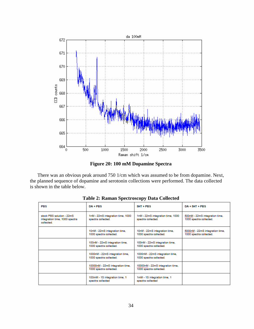
34
Figure 20: 100 mM Dopamine Spectra
There was an obvious peak around 750 1/cm which was assumed to be from dopamine. Next,
the planned sequence of dopamine and serotonin collections were performed. The data collected
is shown in the table below.
Table 2: Raman Spectroscopy Data Collected

35
The data was taken back for analysis. An integration period of 22 ms was used, and 1000 of
these integration periods were collected for each sample. Because of the particular Raman
spectrometer used, over a 22 ms integration period the intensity at each wavelength was a whole
number and corresponded to the “counts” value of the CCD. The CCD counts value represents
the number of electrons produced by the incoming photons. The amount of noise made it
impossible to see any spectra with such low concentration ranges and short integration periods.
Figure 21: A Comparison of the Data from One Integration Period (Top), and Data
Integrated over 1000 of these Periods (Bottom)
After averaging over all 1000 collection periods, some peaks become visible above the noise
floor. The reason that the noise floor shrinks as the number of periods averaged over increase can
be explained as follows. There are 1024 spectral bins 𝑏1, 𝑏2, … , 𝑏1024. Call the CCD count over
one collection period at time 𝑡 for bin 𝑏𝑖 𝑐𝑖𝑡. Call the mean of 𝑐𝑖𝑡 as 𝑡 varies 𝜇𝑖 and the standard
deviation 𝜎𝑖. The central limit theorem tells us that if
𝐶𝑖 ≝1
𝑇∑ 𝑐𝑖𝑡
𝑇
𝑡=1
Then 𝐶𝑖 approaches a normal distribution with mean 𝜇𝑖 and standard deviation 𝜎𝑖
√𝑇. The plot
below shows that the variance of a particular bin can vary wildly.
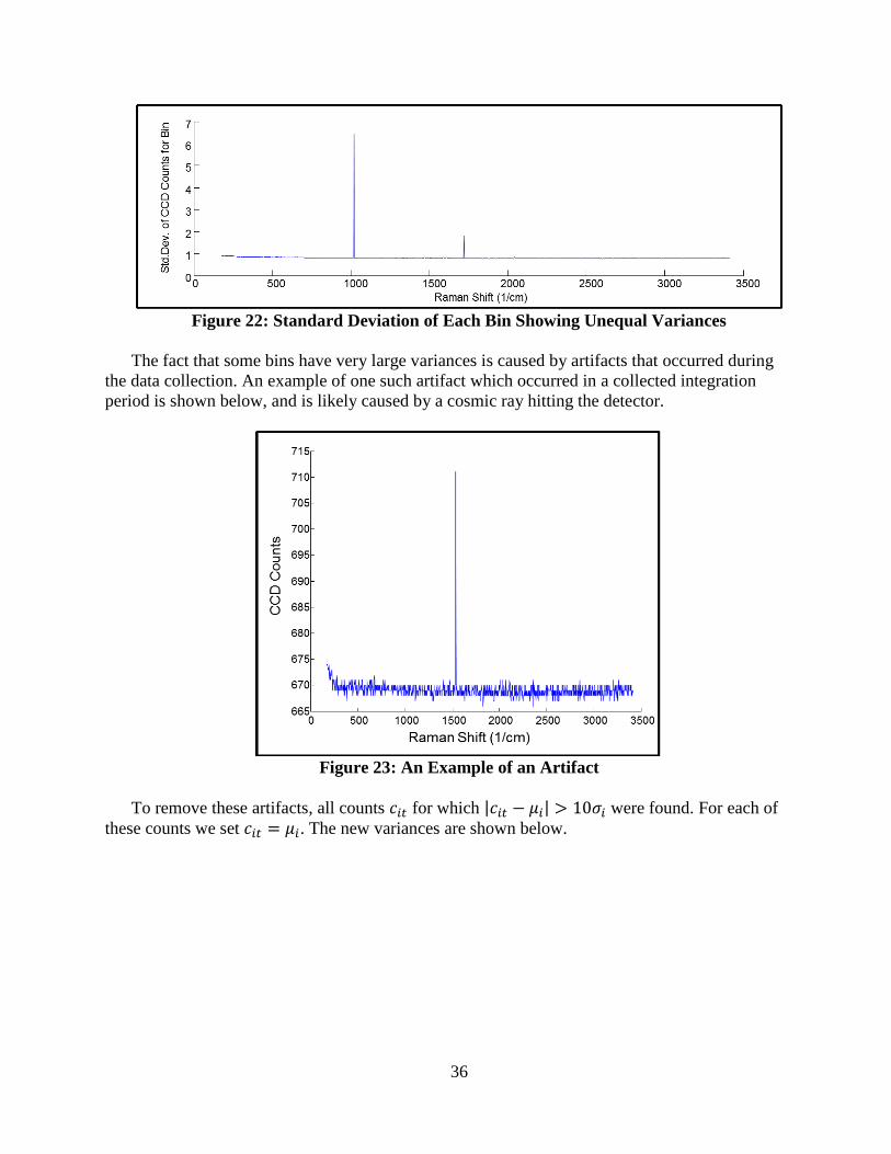
36
Figure 22: Standard Deviation of Each Bin Showing Unequal Variances
The fact that some bins have very large variances is caused by artifacts that occurred during
the data collection. An example of one such artifact which occurred in a collected integration
period is shown below, and is likely caused by a cosmic ray hitting the detector.
Figure 23: An Example of an Artifact
To remove these artifacts, all counts 𝑐𝑖𝑡 for which |𝑐𝑖𝑡 − 𝜇𝑖| > 10𝜎𝑖 were found. For each of
these counts we set 𝑐𝑖𝑡 = 𝜇𝑖. The new variances are shown below.

37
Figure 24: Standard Deviation of Bins after Artifact Removal
It is evident that after the removal of these infrequent artifacts, the variance is practically
constant over all wavelengths of the spectrometer. All of the means were then recalculated 𝜇𝑖 for
this artifact corrected spectra. These post correction 𝜇𝑖’s are plotted below.
Figure 25: Spectra of PBS after Artifact Correction
This gives us a very accurate picture of what the actual Raman spectra of PBS looks like.
You can see a number of distinct peaks caused by molecular resonances. There were no
additional peaks in the Raman spectra observed in data collected for samples containing

38
dopamine or serotonin. The reason that no additional peaks were observed on samples containing
dopamine or serotonin is likely because the signal was too small and not visible above the noise
floor. A concentration of 100 mM dopamine only produced a peak approximately 3 counts above
the background. The next highest concentration collected was 10 uM, meaning that we would
expect this peak to be only 3*10^-4 = 0.0003 counts above the background if the peak height
scales linearly with the concentration of the chemical present.
It was decided that more data collections should be made using even higher concentrations of
dopamine in an attempt to clearly see the spectra of dopamine. Also, it was discovered that the
background of the spectra measured slowly increased over the course of the experiment as if the
equipment was “warming up”. Thus in a second data collection process, the concentrations were
collected in a random order to account for this time varying property of the background. Five
collection sets were acquired, 0-200 nM, 0-1.1 uM, 0-2454.5 uM, and only 2454.5 uM. It was
thought that these concentration ranges would produce clearly visible peaks (0.073635 counts
above the background at 2454.5 uM). However, as will be shown in the results section, no peaks
were visible.
Chapter 4: Results
We sought to test and compare the performance of a univariate model (which actually
consists of two models, a model which only predicts dopamine and a model which only predicts
serotonin) and a multivariate model (consisting of one model which predicts both
neurotransmitters simultaneously) in predicting solutions of dopamine and serotonin.
4.1 Cross Validation
The data was collected on five probes. For each of these five probes there were 81
concentrations of dopamine collected, 81 concentrations of serotonin, 6 pH ranges, and 41
collections with a random mixture of dopamine and serotonin with a random pH level, for a total
of 209 trials for each probe.
A technique known as cross-validation was used to assess the performance of each model
type. To perform cross-validation the dataset was partitioned into three sets, training, validation,
and testing. Three probes were placed into the training set and used to generate the models. One
of the remaining two probes not used for training was used for validation. The alpha and lambda
parameters of the model were varied to produce the minimum prediction error on the validation
probe. Finally, the model along with the alpha and lambda value were used to make predictions
on the test probe and see how well the model performed. This method of cross validation does a
good job of predicting how well the models will perform on new data because the test probe was
not used create the model.
With 5 probes there are 20 ways the data can be partitioned into training, validation, and
testing. For each of the 5 probes chosen as the test probe, there are 4 remaining probes that can
be chosen for the validation probe. We evaluated the performance of the univariate and
multivariate models over all 20 partitions and calculate the average performance of each type of
model.
4.2 Univariate Model

39
The univariate models are actually two models (one for dopamine and one for serotonin).
Each model was trained over a grid of alpha values (0 to 1 in increments of 0.1) and lambda
values (0 to 100 in increments of 1). For each of the training probes (starting with 1 in Figure 26)
we show the predictions of dopamine and serotonin as well as the beta vector generated for each
of the 4 possible validation probes. In the figure showing predictions you can see how the probe
chosen to validate on affected the predictions. Also, two plots which show how the models
confused dopamine and serotonin are shown. The first of these confusion plots shows what
dopamine predictions look like for solutions in which there was no dopamine, only an increasing
amount of serotonin. The second confusion plot shows the same thing, but for serotonin
predictions.
Testing on Probe 1
Average Alpha: 0.675
Average Lambda: 53.5
Variance Alpha: 0.188
Variance Lambda: 2558.8
In Figure 26 you can see how the univariate models did at predicting probe 1. The dopamine
predictions have a positive offset of around 1000-2000 nM, and both dopamine and serotonin
predictions appear to have a smaller slope than the actual slope of the prepared concentrations. In
Figure 27 you can see that the beta vectors are all fairly similar, and they are also quite sparse.
Figure 26: Probe 1 Predictions

40
Figure 27: Betas used for Probe 1 Predictions
In Figure 28 you can see that most of the models seem to interpret an increase in serotonin
levels as a decrease in dopamine levels. Also, in Figure 29 you can see that an increase in
dopamine is causes an increase in serotonin predictions at low dopamine concentrations and a
decrease in serotonin predictions at high dopamine concentrations.
Figure 28: Increasing Serotonin Confusion Plot

41
Figure 29: Increasing Dopamine Confusion Plot
Testing on Probe 2
Average Alpha: 0.85
Average Lambda: 75.75
Variance Alpha: 0.212
Variance Lambda: 2911.8
In Figure 30 it is evident that the vertical offset is much lower than for probe 1. Also, most of the
predictions appear to be very accurate, though there is a lot of variation. For both dopamine and
serotonin, validating on probe 1 seemed to produce the worst predictions. In Figure 31 you can
see that the beta vector produced by validating on probe 1 has many more nonzero entries than
the other beta vectors.

42
Figure 30: Probe 2 Predictions
Figure 31: Betas used for Probe 2 Predictions
Confusion plots for dopamine predictions (Figure 32) and serotonin predictions (Figure 33)
on probe 2 show that as the alternate chemical varies concentration, the predicted chemical
varies little. This means that these predictions are less likely to confuse a change in dopamine for
a change in serotonin and vice versa.

43
Figure 32: Increasing Serotonin Confusion Plot
Figure 33: Increasing Dopamine Confusion Plot
Testing on Probe 3
Average Alpha: 0.55
Average Lambda: 62
Variance Alpha: 0.173
Variance Lambda: 2336.3
Testing on probe 3 produced very poor results. You can see that the dopamine predictions
hardly changed at all as the actual concentration varied in Figure 34. The serotonin predictions

44
varied more, but there was a large offset error. The betas in Figure 35 are also very noisy, with
many nonzero entries.
Figure 34: Probe 3 Predictions
Figure 35: Betas used to Predict Probe 3
The confusion plots in Figure 36 and Figure 37 indicate the models do not confuse the
chemicals easily, but this is just because the output of the models is always very close to 0
regardless of the actual concentration.

45
Figure 36: Increasing Serotonin Confusion Plot
Figure 37: Increasing Dopamine Confusion Plot
Testing on Probe 4
Average Alpha: 0.925
Average Lambda: 49.5
Variance Alpha: 0.1880
Variance Lambda: 1666.3
The predictions on probe 4 are extremely good. In Figure 38 there is almost no vertical offset
error, and the slope is very close to the true concentration slope. The beta vectors in Figure 39 all

46
look very similar, with peaks corresponding the oxidation and reduction regions of the
voltammagram.
Figure 38: Probe 4 Predictions
Figure 39: Betas used to Predict Probe 4
The confusion plots in Figure 40 and in Figure 41 also show the near ideal behavior of this
mode. There is a clear distinction between the two chemicals.

47
Figure 40: Increasing Serotonin Confusion Plot
Figure 41: Increasing Dopamine Confusion Plot
Testing on Probe 5
Average Alpha: 0.575
Average Lambda: 64.75
Variance Alpha: 0.1092
Variance Lambda: 2236.9
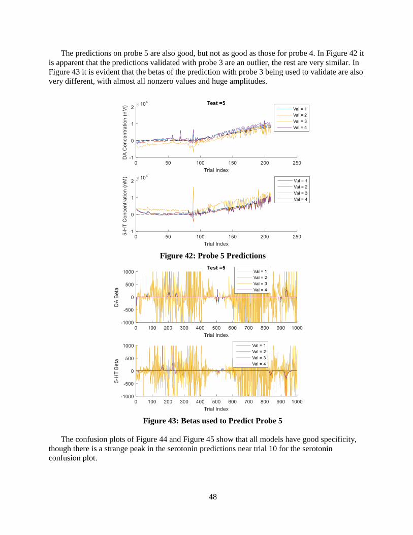
48
The predictions on probe 5 are also good, but not as good as those for probe 4. In Figure 42 it
is apparent that the predictions validated with probe 3 are an outlier, the rest are very similar. In
Figure 43 it is evident that the betas of the prediction with probe 3 being used to validate are also
very different, with almost all nonzero values and huge amplitudes.
Figure 42: Probe 5 Predictions
Figure 43: Betas used to Predict Probe 5
The confusion plots of Figure 44 and Figure 45 show that all models have good specificity,
though there is a strange peak in the serotonin predictions near trial 10 for the serotonin
confusion plot.
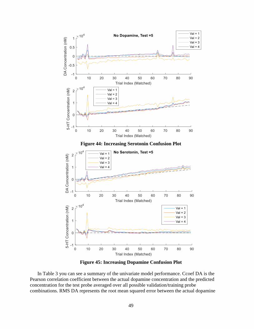
49
Figure 44: Increasing Serotonin Confusion Plot
Figure 45: Increasing Dopamine Confusion Plot
In Table 3 you can see a summary of the univariate model performance. Ccoef DA is the
Pearson correlation coefficient between the actual dopamine concentration and the predicted
concentration for the test probe averaged over all possible validation/training probe
combinations. RMS DA represents the root mean squared error between the actual dopamine
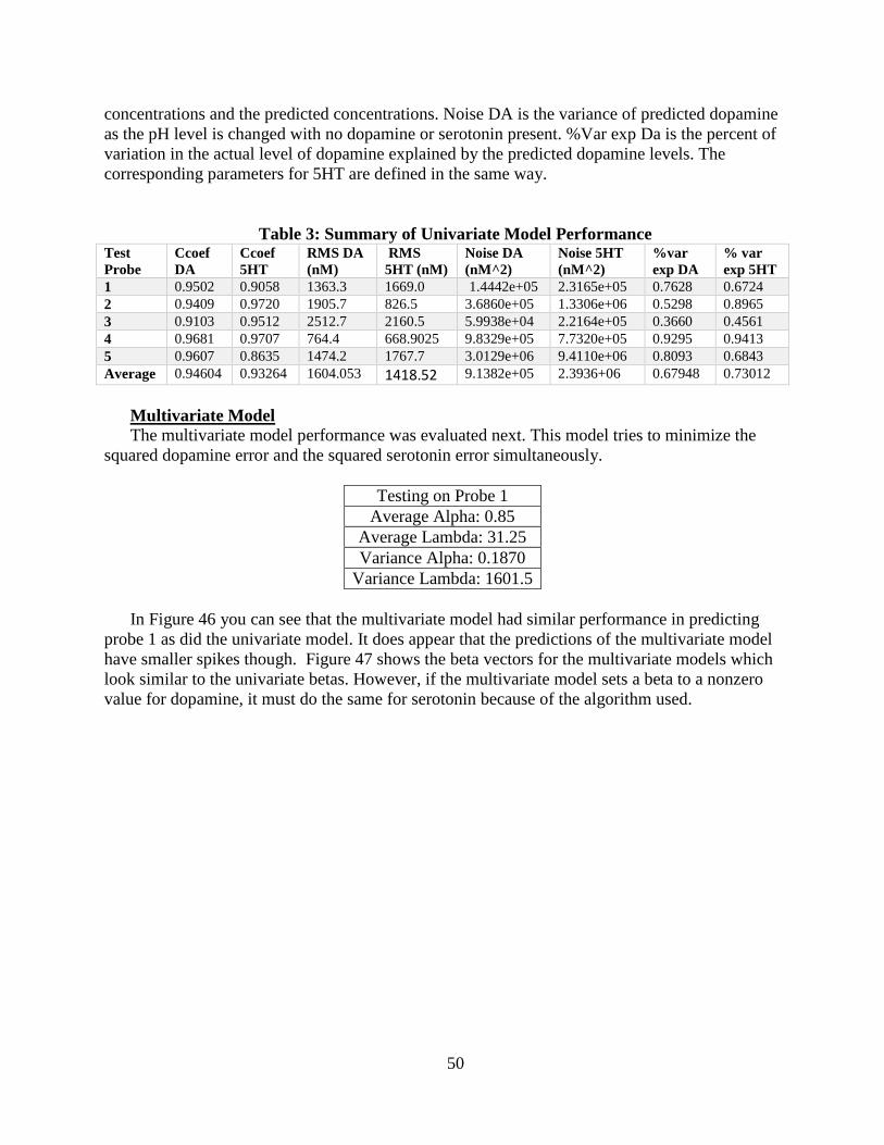
50
concentrations and the predicted concentrations. Noise DA is the variance of predicted dopamine
as the pH level is changed with no dopamine or serotonin present. %Var exp Da is the percent of
variation in the actual level of dopamine explained by the predicted dopamine levels. The
corresponding parameters for 5HT are defined in the same way.
Table 3: Summary of Univariate Model Performance Test
Probe
Ccoef
DA
Ccoef
5HT
RMS DA
(nM)
RMS
5HT (nM)
Noise DA
(nM^2)
Noise 5HT
(nM^2)
%var
exp DA
% var
exp 5HT
1 0.9502 0.9058 1363.3 1669.0 1.4442e+05 2.3165e+05 0.7628 0.6724
2 0.9409 0.9720 1905.7 826.5 3.6860e+05 1.3306e+06 0.5298 0.8965
3 0.9103 0.9512 2512.7 2160.5 5.9938e+04 2.2164e+05 0.3660 0.4561
4 0.9681 0.9707 764.4 668.9025 9.8329e+05 7.7320e+05 0.9295 0.9413
5 0.9607 0.8635 1474.2 1767.7 3.0129e+06 9.4110e+06 0.8093 0.6843
Average 0.94604 0.93264 1604.053 1418.52 9.1382e+05 2.3936+06 0.67948 0.73012
Multivariate Model
The multivariate model performance was evaluated next. This model tries to minimize the
squared dopamine error and the squared serotonin error simultaneously.
Testing on Probe 1
Average Alpha: 0.85
Average Lambda: 31.25
Variance Alpha: 0.1870
Variance Lambda: 1601.5
In Figure 46 you can see that the multivariate model had similar performance in predicting
probe 1 as did the univariate model. It does appear that the predictions of the multivariate model
have smaller spikes though. Figure 47 shows the beta vectors for the multivariate models which
look similar to the univariate betas. However, if the multivariate model sets a beta to a nonzero
value for dopamine, it must do the same for serotonin because of the algorithm used.

51
Figure 46: Probe 1 Predictions
Figure 47: Betas used to Predict Probe 1
In Figure 48 and Figure 49 you can see that the confusion plots for the multivariate model are
almost identical to the univariate model confusion plots for probe 1.
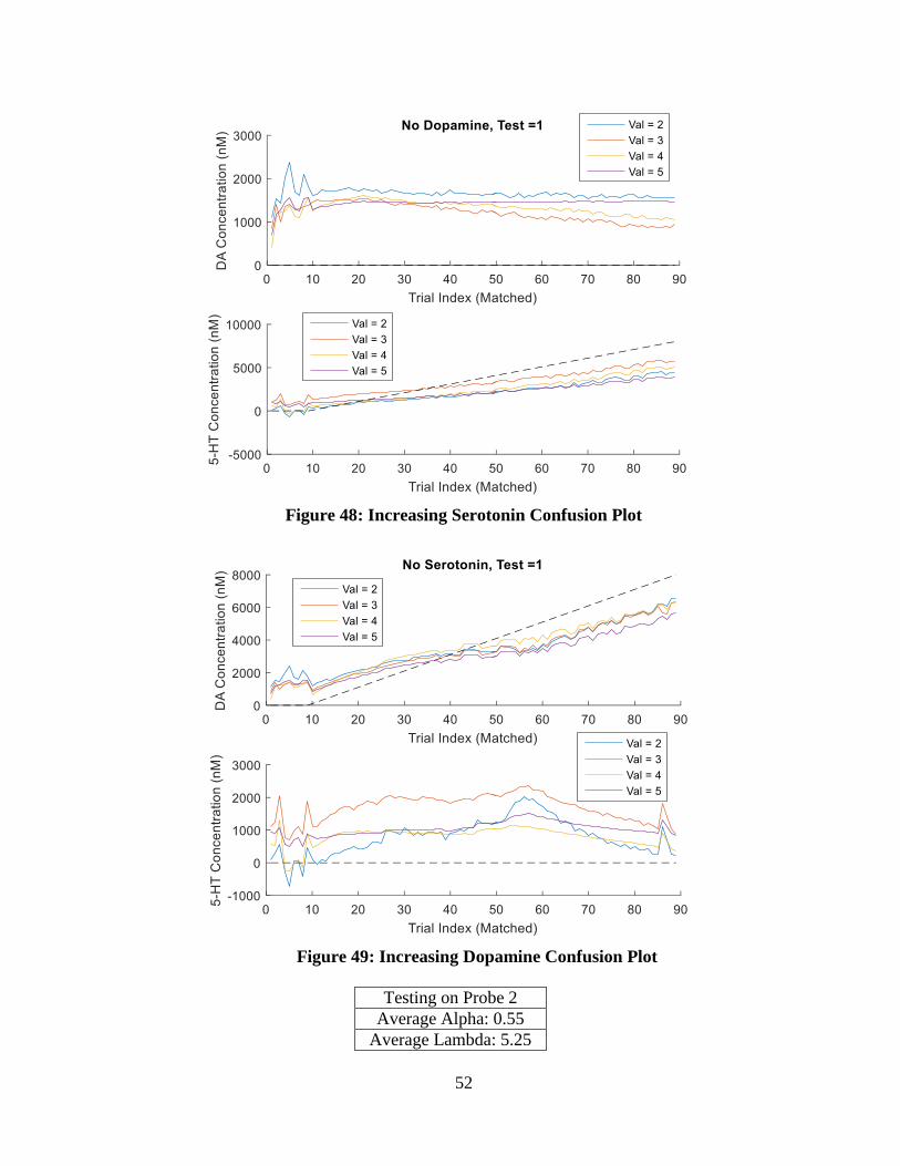
52
Figure 48: Increasing Serotonin Confusion Plot
Figure 49: Increasing Dopamine Confusion Plot
Testing on Probe 2
Average Alpha: 0.55
Average Lambda: 5.25

53
Variance Alpha: 0.2230
Variance Lambda: 19.70
The predictions for probe 2 are better than the predictions for probe 1, except when
validation probe 1 is used as shown in Figure 50. The betas shown in Figure 51 have a very
smooth appearance that is not very sparse except for the betas for validation on probe 1 which
are very spiky looking.
Figure 50: Probe 2 Predictions
Figure 51: Betas used to Predict Probe 2

54
The confusion plots in Figure 52 and Figure 53 show that at low concentrations the models
have poor specificity, but the specificity improves as the concentration of the chemical of interest
increases.
Figure 52: Increasing Serotonin Confusion Plot
Figure 53: Increasing Dopamine Confusion Plot
Testing on Probe 3

55
Average Alpha: 0.9
Average Lambda: 42
Variance Alpha: 0.1920
Variance Lambda: 2046.3
The predictions for probe 3 are very poor, as they are for the univariate model. Figure 54
shows the poor sensitivity of dopamine predictions and the offset of the serotonin predictions.
Figure 55 shows that the betas are also quite noisy looking in the sense that the location of
nonzero elements appear to be somewhat random.
Figure 54: Probe 3 predictions
Figure 55: Betas used to Predict Probe 3

56
The dopamine predictions have a slightly negative slope as the serotonin concentrations
increase as can be seen in Figure 56. The serotonin predictions in Figure 57 are fairly flat, but
have a vertical offset.
Figure 56: Increasing Serotonin Confusion Plot

57
Figure 57: Increasing Dopamine Confusion Plot
Testing on Probe 4
Average Alpha: 0.675
Average Lambda: 46.25
Variance Alpha: 0.2580
Variance Lambda: 2431.5

58
The predictions on probe 4 are very good for the multivariate model as can be seen Figure
58. The betas are also very clean looking as can be seen in Figure 59. It appears that there are
two large positive peaks in the first half of the waveform for serotonin and only one for
dopamine.
Figure 58: Probe 4 Predictions
Figure 59: Betas used to Predict Probe 4

59
The confusion plots in Figure 60 and Figure 61 show that despite a few horizontal offsets, the
dopamine predictions are not heavily affected by the serotonin concentrations and the serotonin
concentrations are not heavily affected by the dopamine concentrations.
Figure 60: Increasing Serotonin Confusion Plot
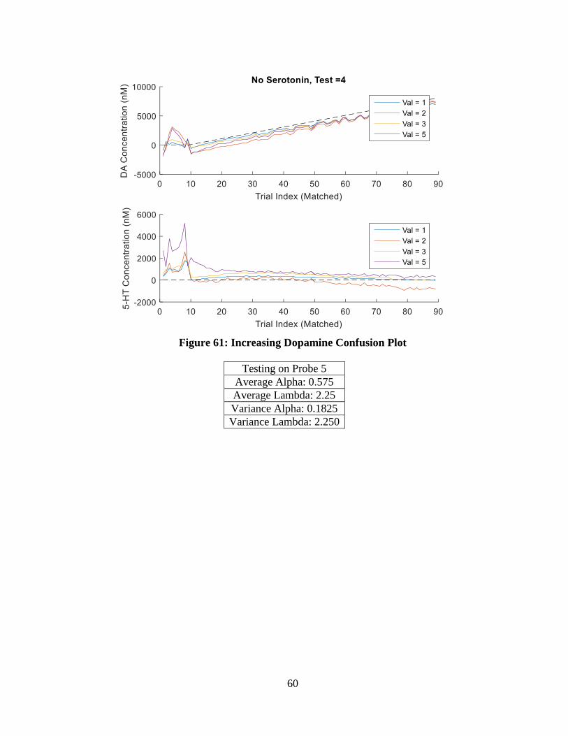
60
Figure 61: Increasing Dopamine Confusion Plot
Testing on Probe 5
Average Alpha: 0.575
Average Lambda: 2.25
Variance Alpha: 0.1825
Variance Lambda: 2.250

61
The predictions for probe 5 are shown in Figure 62 and the betas are shown in Figure 63. The
predictions look fairly accurate, as well as the betas except for when probe 3 is used for
validation.
Figure 62: Probe 5 Predictions
Figure 63: Betas used to Predict Probe 5
The confusion plots shown in Figure 64 and Figure 65 show that all models have good
specificity. Even the predictions when validating on probe 3 are have fairly good specificity.

62
Figure 64: Increasing Serotonin Confusion Plot
Figure 65: Increasing Dopamine Confusion Plot
In Table 4 we have listed the summary of the multivariate model performance. These are the
same parameters are reported for the univariate model performance.

63
Table 4: Summary of Multivariate Model Performance Test
Probe
Ccoef
DA
Ccoef
5HT
RMS DA
(nM)
RMS 5HT
(nM)
Noise DA
(nM^2)
Noise 5HT
(nM^2)
%var
exp DA
% var
exp 5HT
1 0.9673 0.9244 1369.4 1659.2 9.2155e+04 1.8704e+05 0.7471 0.6500
2 0.9445 0.9734 18043 1012.3 4.3936e+05 5.1064e+05 0.5607 0.8708
3 0.9191 0.9437 2395.1 2176.4 2.4672e+04 2.6905e+05 0.3615 0.4414
4 0.9702 0.9725 754.9904 699.0870 1.3479e+06 5.7749e+05 0.9313 0.9379
5 0.9611 0.8689 1467.3 2266.6 1.5914e+06 1.4071e+06 0.7205 0.6779
Average 0.95244 0.93658 1558.218 15627.2 6.9909e+05 5.9026e+05 0.66422 0.7156
Looking at the predictions of the multivariate and univariate models we can see that the
performance of the two is almost identical in our test with the multivariate model having a higher
linear correlation coefficient and the univariate model explaining a slightly higher percentage of
the variance. Interestingly though, the noise of the multivariate model calculated on the pH only
trials is much lower than the univariate model. This is really what sets the two models apart. The
multivariate model seems to be less affected by noise factors such as pH as shown in Figure 66.
Figure 66: Comparison of Noise
Model Sensitivity Analysis
The next analysis performed was intended to determine the relative sensitivity of the
univariate and multivariate models. To determine this 10%, 50%, and then 90% of the betas were
zeroed and then used to make predictions. It was also desired to see how the sensitivity of these
models varied as a function of the concentration of chemical present. Therefore, the
concentration ranges were divided into low (where concentrations of dopamine or serotonin were

64
from 100 to 1000 uM), medium (where concentrations of dopamine or serotonin were from 1100
to 4000 uM), and high (where concentrations of dopamine or serotonin are at least 4100 uM).
Univariate Model Performance
10% zeroed Ccoef DA Ccoef 5-HT
Low (100-1000 uM) 0.1116 0.1917
Medium (1100-4000 uM) 0.9220 0.3354
High (4100-8000 uM) 0.5769 0.5160
RMS DA RMS 5-HT
Low (100-1000 uM) 7.3402e+03 2.0802e+04
Medium (1100-4000 uM) 7.3019e+03 2.2392e+04
High (4100-8000 uM) 7.7071e+03 2.2701e+04
50% zeroed Ccoef DA Ccoef 5-HT
Low (100-1000 uM) 0.2349 0.0676
Medium (1100-4000 uM) 0.7088 0.6050
High (4100-8000 uM) 0.2794 0.8359
RMS DA RMS 5-HT
Low (100-1000 uM) 3.4374e+04 1.6591e+04
Medium (1100-4000 uM) 3.4292e+04 1.7342e+04
High (4100-8000 uM) 3.2731e+04 1.8377e+04
90% zeroed Ccoef DA Ccoef 5-HT
Low (100-1000 uM) -0.0051 -0.1646
Medium (1100-4000 uM) 0.7171 -0.2188
High (4100-8000 uM) 0.7588 -0.5498
RMS DA RMS 5-HT
Low (100-1000 uM) 9.0627e+03 2.1827e+04
Medium (1100-4000 uM) 7.9866e+03 2.4450e+04
High (4100-8000 uM) 6.3909e+03 2.8570e+04
Multivariate Model Performance
10% zeroed Ccoef DA Ccoef 5-HT
Low (100-1000 uM) -0.0156 0.1516
Medium (1100-4000 uM) 0.9570 0.2101
High (4100-8000 uM) 0.6487 0.5377
RMS DA RMS 5-HT
Low (100-1000 uM) 4.0006e+03 1.8082e+03

65
Medium (1100-4000 uM) 4.2635e+03 1.6867e+03
High (4100-8000 uM) 4.6434e+03 2.4955e+03
50% zeroed Ccoef DA Ccoef 5-HT
Low (100-1000 uM) 0.0431 0.1541
Medium (1100-4000 uM) 0.8294 0.2112
High (4100-8000 uM) 0.6507 0.5089
RMS DA RMS 5-HT
Low (100-1000 uM) 1.5237e+03 1.5720e+03
Medium (1100-4000 uM) 856.0890 2.5633e+03
High (4100-8000 uM) 2.6414e+03 4.7556e+03
90% zeroed Ccoef DA Ccoef 5-HT
Low (100-1000 uM) 0.1555 -0.1513
Medium (1100-4000 uM) 0.4631 0.1210
High (4100-8000 uM) 0.4792 0.2779
RMS DA RMS 5-HT
Low (100-1000 uM) 1.0789e+04 1.1540e+04
Medium (1100-4000 uM) 9.1572e+03 1.3702e+04
High (4100-8000 uM) 6.1737e+03 1.6890e+04
The preceding sensitivity analysis revealed that at some point zeroing more of the betas does
not further increase the RMS error. This is because the mean offset of the model is not included
in the betas which can be zeroed. When all of the other betas are zeroed the predictions will just
be a constant equal to the mean of the training data. Figure 67 shows that the RMS error
decreased for the univariate DA and the multivariate 5HT when the percentage was increased
from 50% zeroed to 90%.

66
Figure 67: RMS Error as Function of Percent of Beta Zeroed
Simulated Raman Spectroscopy Data
As stated before, there was no visible signal from dopamine or serotonin the data collected. It
is unclear why this occurred, as the highest concentrations data was collected on should have in
theory produced visible peaks. In the paper titled “Detection and Monitoring of
Neurotransmitters - a Spectroscopic Analysis” [38] Raman spectroscopy is performed on
dopamine, serotonin, and adenosine. An excitation wavelength of 532 nm was used. 100 μM
concentrations were prepared of each. There are several peaks visible in the measured spectra of
each chemical from this study. Even taking into account the fact that signals are approximately
4.7 times greater at 532 nm than they are at 785 nm, it would seem that there should be peaks
seen at the high concentration ranges our data was collected at as well.
It is unlikely that the wrong concentration was mixed and placed into the quartz flow cell. A
more likely cause is that either the focal plane of the microscope wasn’t aligned with the interior
of the flow cell causing the spectra of the quartz flow cell to be seen instead of the spectra of the
solution inside of the flow cell, or that the Raman scattering was weaker at this wavelength than
expected from theory.
Whatever the cause, no data allowing the spectra of dopamine or serotonin to be determined
was obtained from the Raman data collection at Virginia Tech. Therefore, in order to try out the
elastic net algorithm on Raman spectroscopy data, it was necessary to make simulated Raman
spectra. To make these simulated Raman spectra, a model very similar to that of the generative
model made for FSCV data was used. It was assumed that the total observed spectra was equal to
the background spectra, the AWGN noise, and the spectra from dopamine and serotonin. The
spectra from dopamine and serotonin was assumed to be proportional to the concentration of
each.

67
Figure 68: Components of Simulated Raman Spectra
There were a few important differences however between the two models. For one, the
background current was not assumed to vary for the Raman model as it was with the FSCV
model. This assumption appears to be fairly accurate based on the Raman data collected. There is
a horizontal shift in the background which slowly varied during the course of the experiment, but
the actual shape of the background spectra does not appear to vary. The height of the peaks was
based off the results presented by Manciu et al. [38]. The spectral contribution of 1uM dopamine
is shown in Figure 69 and the contribution of 1uM serotonin is shown in Figure 70.
Figure 69: Spectral Contribution of 1uM Dopamine

68
Figure 70: Spectral Contribution of 1uM Serotonin
Using the above spectra for dopamine and serotonin, the simulated data was generated in
three concentration ranges spanning 3 orders of magnitude.
Low – 0, 0.05uM, 0.25uM, and 0.5uM
Medium – 0, 0.5uM, 2.5uM, and 5uM
High – 0, 5uM, 25uM, and 50uM
In the following set of figures you can see what a simulated spectra for the low, medium, and
high concentration ranges would look like (i.e. no visible peaks). The dopamine and serotonin
spectra are scaled according to the amount of each present and then noise and the background
PBC spectra are added in.
Low (dopamine on top, serotonin on bottom) - 0.5uM spectra

69
Figure 71: 0.5uM Dopamine Spectra
Figure 72: 0.5uM Serotonin Spectra
Medium (dopamine on left, serotonin on right) - 5uM spectra
Figure 73: 5uM Dopamine Spectra

70
Figure 74: 5uM Serotonin Spectra
High (dopamine on left, serotonin on right) - 50uM spectra
Figure 75: 50uM Dopamine Spectra
Figure 76: 50uM Serotonin Spectra
Now we use these simulated Raman spectra to train univariate models and multivariate models
and see how they perform at low, medium, and high concentration ranges.
Univariate Model

71
The univariate model was trained first. You can see the performance of this model both by
examining the betas and the table.
Low – 0, 0.05uM, 0.25uM, and 0.5uM
The best alpha was found to be 0 (corresponding to a pure 𝑙1 norm penalty) through cross
validation and the best lambda was found to be 1.927. At these low concentration ranges, the
model fails to identify any of the Raman peaks at all is thus unable to predict concentrations at
these low ranges.
Figure 77: Low Concentration Dopamine Beta
Figure 78: Low Concentration Serotonin Beta
Medium - 0, 0.5uM, 2.5uM, and 5uM
The best alpha was found to be 0.4 through cross validation and the best lambda was found to be
0.1549. At these concentration ranges the model appears to find more than half of the Raman
spectral peaks present in the signal.

72
Figure 79: Medium Concentration Dopamine Beta
Figure 80: Medium Concentraiton Serotonin Beta
High - 0, 5uM, 25uM, and 50uM
The best alpha was found to be 0 and the best lambda was found to be 37.479. At this highest
range the model is able to detect practically all of the Raman spectral peaks.

73
Figure 81: High Concentration Dopamine Beta
Figure 82: High Concentration Serotonin Beta
The univariate performance results are summarized in the following tables. These tables
describe the same Ccoef and RMS parameters as were used with the fast-scan cyclic
voltammetry section. The cross correlation coefficient is also reported, with Cross Correlation
Coefficient DA/5-HT representing the correlation between dopamine predictions and the actual
value of serotonin. The Cross Correlation Coefficient 5-HT/DA represents the correlation
between serotonin predictions and the actual value of dopamine present.
Ccoef DA Ccoef 5-HT
Low -0.5639 -0.0226 Medium 0.8808 0.9536 High 0.9993 0.9998
Cross Correlation Coefficient
DA/5-HT
Cross Correlation Coefficient 5-
HT/DA
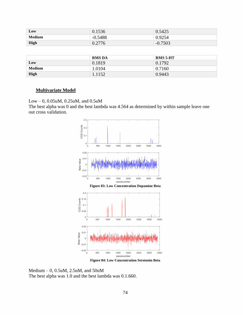
74
Low 0.1536 0.5425 Medium -0.5488 0.9254 High 0.2776 -0.7503
RMS DA RMS 5-HT
Low 0.1819 0.1792 Medium 1.0104 0.7160 High 1.1152 0.9443
Multivariate Model
Low – 0, 0.05uM, 0.25uM, and 0.5uM
The best alpha was 0 and the best lambda was 4.564 as determined by within sample leave one
out cross validation.
Figure 83: Low Concentration Dopamine Beta
Figure 84: Low Concentration Serotonin Beta
Medium – 0, 0.5uM, 2.5uM, and 50uM
The best alpha was 1.0 and the best lambda was 0.1.660.

75
Figure 85: Medium Concentration Dopamine Beta
Figure 86: Medium Concentration Serotonin Beta
High – 0, 0.5uM, 2.5uM, and 50uM
The best alpha was 0.8 and the best lambda was 0.381.
Figure 87: High Concentration Dopamine Beta

76
Figure 88: High Concentration Serotonin Beta
Ccoef DA Ccoef 5-HT
Low -0.0157 -0.0889 Medium 0.8997 0.9659 High 0.9996 0.9990
Cross Correlation Coefficient
DA/5-HT
Cross Correlation Coefficient 5-
HT/DA
Low 0.6932 -0.5110 Medium -0.8784 0.2156 High -0.5086 0.3331
RMS DA RMS 5-HT
Low 0.1833 0.1842 Medium 0.8047 0.4745 High 0.7017 0.8434
As can be seen in Figure 89, the univariate and multivariate models again have similar
performance characteristics. It seems that especially with this simulated Raman spectroscopy
data the transition from a readable signal to one too corrupted by noise is very fast.

77
Figure 89: Correlation Coefficient vs. Concentration
Chapter 5: Conclusion
This work extends the work on fast-scan cyclic voltammetry by testing whether mixtures of
two substances with similar oxidation and reduction profiles can be recovered using a supervised
learning approach. Previous studies only reported relative changes in dopamine by observing a
qualitative shift in the oxidation and reduction curves. I have shown that it is possible to obtain
quantitative concentrations of dopamine and serotonin at the same time with only one
measurement with certain error tolerances.
5.1 Summary of work
Monoamine neurotransmitters such as dopamine and serotonin have been extensively studied
in animals and humans, however their exact role and function is still poorly understood. For the
first time, fast scan cyclic voltammetry measurements have been recorded from the striatum of
human patients who were playing a probabilistic decision making task. These measurements
contain information about the release of neurotransmitters including dopamine and serotonin that
have never been studied with such high time resolution in humans. I developed, advanced signal
processing and machine learning techniques to test whether this sort of patient data could be
interrogated for concentration transients of both dopamine and serotonin.
Confocal Raman spectroscopy data was collected on prepared samples of dopamine and
serotonin in vitro. This data revealed that very high concentrations of both are necessary to be
detected with standard Raman spectroscopy. Also, the same elastic net signal reconstruction and
regression techniques that were applied to the FSCV data were applied to the Raman data. With

78
simulated data, it was shown that these techniques are able to determine individual Raman
spectra from a noisy mixture of sources and convert a Raman spectrum into concentrations of
each mixture component present.
The most commonly chosen value of alpha was 1.0 for both fast-scan cyclic voltammetry
data as well as Raman spectroscopy data as determined by cross validation. This corresponds to
the Lasso regression analysis method. A few alphas were found to be lower values, but most
were still near 1.0. This is likely caused by the fact that both signals are sparse and alpha values
close to 1.0 force more of the beta elements to be 0.
The performance of the univariate and multivariate models was very similar on the fast-scan
cyclic voltammetry data. However, the multivariate model appeared to reduce the signal noise
caused by pH changes.
5.2 Future Directions
In the article Fourier transform Raman spectroscopy [42] published in 1986, the author states
that one of the biggest problem with the routine application of Raman spectroscopy is the
interference caused by fluorescence of impurities or of the sample itself. One solution is to use
long-wavelength near-infrared lasers such as a Nd/YAG laser operating at 1.064 um. The longer
wavelength means that fluorescence is drastically reduced. However, two new problems arise.
First, the Raman signal at this longer wavelength is approximately 1/16 of the signal present at
514.5 nm because it decreases in proportion to the fourth power of the wavelength. Also,
available detectors in this region are much noisier than photomultipliers. Eight years later
Mizuno et al. [43] used Fourier transform Raman spectroscopy to obtain high quality Raman
spectra of human brain tissues and several kinds of brain tumors. The authors mention that
Raman spectroscopy is one the most powerful non-invasive probes for investigating biological
materials at the molecular level. They mention two major disadvantages of Raman spectroscopy,
interference by fluorescence of the tissue (mentioned in the 1986 article above) and the
decomposition of biological materials caused by the heating of the laser beam. They decide to
use Fourier transform Raman spectroscopy because it overcomes the mentioned two
disadvantages. Acceptable spectra were obtained in the range of 400-2970 cm^-1. In the article
by Katz et al. [44], a method known as compressed sensing i applied to Fourier-transform Raman
spectroscopy. The compressed sensing techniques they apply allow for a considerable reduction
in the acquisition time. They demonstrate the technique on coherent anti-Stokes Raman
scattering spectroscopy and show that it is possible to resolve sparse vibrational spectra using
<25% of the Nyquist rate samples in single pulse CARS experiments. They say that in FT
spectroscopy, a set of N equally spaced time-domain measurements are made. Raman spectra are
sparse, which means that compressed sensing techniques can be applied to reduce the number of
samples necessary. The CARS data they looked at was composed of N=281 equally spaced
measurements. They chose M<N points at random and used them as the input for a CS
reconstruction algorithm. They found that M~>60 samples was all that was needed to accurately
resolve the Raman lines. Therefore, it is proposed that compressed sensing and Fourier transform
Raman spectroscopy be combined to make a probe capable of measuring neurochemical levels in
vivo. The probe would operate in the infrared region of 1.064 um allowing for the fluorescence
of brain tissue to be almost completely eliminated. Because detectors are difficult to manufacture
which are sensitive to this long wavelength, Fourier transform Raman could be used to allow a
single element detector to be used instead of the detector arrays and CCD arrays needed for
traditional spectrometers. To reduce collection time to sub-second timescales, compressed

79
sensing techniques would be used to sample the Raman spectra over a small subset of randomly
spaced Fourier coefficients. L1-norm reconstruction techniques could then be used to recreate
the Raman spectra from a very small number of Fourier components. Raman spectra are perfect
for compressed sensing strategies because the spectra are very sparse. Except for shifts at a few
discrete molecular resonances, the Raman spectra are zero at most wavenumbers.
References
[
1]
K. Kishida, S. Sandberg, T. Lohrenz, Y. Comair, I. Sáez and e. al., "Sub-Second
Dopamine Detection in Human Striatum," PLoS ONE, 2011.
[
2]
P. Cranefield, "Action potentials, afterpotentials, and arrhythmias," Circulation
Research, pp. 415-423, 1977.
[
3]
S. Robinson, "Firing properties of dopamine neurons in freely moving dopamine-
deficient mice: effects of dopamine receptor activation and anesthesis.".
[
4]
US National Institutes of Health, Chemical synapse schema cropped, 2009.
[
5]
"Neuroscience web page," [Online]. Available:
http://ai.ato.ms/MITECS/Front/neuroscience.html.
[
6]
D. Pelvig, "Neocortical glial cell numbers in human brains," Neurobiology of aging, p.
1754, 2008.
[
7]
National Institutes of Health, Dopamine pathways, 2012.
[
8]
P. Calabresi, "DIrect and indirect pathways of basal ganglia. a critical reappraisal,"
Nature Neuroscience, p. 1022, 2014.
[
9]
W. Schultz, "A neural substrate of prediction and reward," Science, p. 1593, 1997.
[
10]
R. Goldstein, "Drug addiction and its underlying neurobiological basis: Neuroimaging
evidence for the involvement of the frontal cortex," The Americal journal of psychiatry, p.
1642, 2002.
[
11]
I. Tork, "Anatomy of the serotonergic system," Annals of the New York Academy of
Sciences, p. 600, 1990.
[
12]
National Institutes of Health, equitativa hormonal, 2015.
[
13]
P. Dayan, "Serotonin in Affective Control," Annual review of neuroscience, p. 95, 2009.
[
14]
D. Hoyer, D. E. Clarke, J. R. Fozard, P. R. Hartig, G. R. Martin, E. J. Mylecharane, P.
R. Saxena and P. P. Humphrey, "International Union of Pharmacology classification of
receptors for 5-hydroxytryptamine (Serotonin)," Pharmacological reviews, pp. 157-203,
1994.
[
15]
D. Sibley, "Molecular biology of dopamine receptors," Trends in pharmacological
sciences, p. 61, 1992.
[
16]
M. Asberg, ""Serotonin depression"-- a biochemical subgroup within the affective
disorders?," Science, p. 478, 1976.

80
[
17]
D. P. Huys, "Serotonin, Inhibition, and Negative Mood.," PLos Comput Biol, 2008.
[
18]
J. Deakin and F. Graeff, "5-HT and mechanisms of defence," Psychopharmacol, pp.
305-316, 1991.
[
19]
D. Nathaniel, "Opponent interactions between serotonin and dopamine," Neural
Networks, p. 603, 2002.
[
20]
"Hyperphysics," [Online]. Available: hyperphysics.phy-
astr.gsu.edu/hbase/nucene/nucmed.html.
[
21]
J. Maus, PET-schema, 2003.
[
22]
F. Cicchetti, ": Neuroinflammation of the nigrostriatal pathway during progressive 6-
OHDA dopamine degeneration in rats monitored by immunohistochemistry and PET
imaging," The European journal of neuroscience, p. 991, 2002.
[
23]
B. Le Foll, D. Payer and P. Di Ciano, "Occupancy of Dopamine D3 and D2 Receptors
by Busiprone: A [11C]-(+)-PHNO PET study in humans," Neuropsychopharmacology, pp.
529-537, 2016.
[
24]
"What is fMRI," [Online]. Available: http://fmri.ucsd.edu/Research/whatisfmri.html.
[
25]
K. S. Wang, D. V. Smith and M. R. Delgado, "Using fMRI to Study Reward Processing
in Humans: Past, Present, and Future," Journal of neurophysiology, p. 333, 2016.
[
26]
G. de Hollander, M. C. Keuken and B. U. Forstmann, "The Subcortical Cocktail
Problem; Mixed Signals from the Subthalamic Nucleus and Substantia Nigra.," PloS one, p.
18, 2015.
[
27]
Y. C. I. Chen, W. R. Galpern, A. L. Brownell, R. T. Matthews, M. Bogdanov, O.
Isacson and B. G. Jenkins, "Detection of dopaminergic neurotransmitter activity using
pharmacologic MRI: correlation with PET, microdialysis, and behavioral data.," Magnetic
Resonance in Medicine, pp. 389-398, 1997.
[
28]
M. G. Shapiro, G. G. Westmeyer, P. A. Romero, J. O. Szablowski, B. Küster, A. Shah
and A. Jasanoff, "Directed evolution of a magnetic resonance imaging contrast agent for
noninvasive imaging of dopamine.," Nature biotechnology, pp. 264-270, 2010.
[
29]
R. B. Rutledge, M. Dean, A. Caplin and P. W. Glimcher, "Testing the reward prediction
error hypothesis with an axiomatic model.," The Journal of Neuroscience, pp. 13525-13536,
2010.
[
30]
A. Caplin and M. Dean, "Axiomatic methods, dopamine and reward prediction error,"
Current opinion in neurobiology, pp. 197-202, 2008.
[
31]
F. Blandini and M. T. Armentero, "Animal models of Parkinson’s disease," FEBS
Journal, pp. 1156-1166, 2012.
[
32]
W. R. Gibb and A. J. Lees, "The relevance of the Lewy body to the pathogenesis of
idiopathic Parkinson's disease.," Journal of Neurology, Neurosurgery & Psychiatry, pp.
745-752, 1988.
[
33]
I. Morales, A. Sanchez, C. Rodriguez-Sabate and M. Rodriguez, "The degeneration of
dopaminergic synapses in Parkinson's disease: A selective animal model.," Behavioural
brain research, pp. 19-28, 2015.

81
[
34]
H. A. Laitinen and I. M. Kolthoff, "Voltammetry with Stationary Microelectrodes of
Platinum Wire," The Journal of Physical Chemistry, vol. 45, pp. 1061-1079, 1941.
[
35]
A. Michael and L. Borland, Electrochemical Methods for Neuroscience, Boca Raton:
CRC Press/Taylor & Francis, 2007.
[
36]
A. S. R. R. B. G. P. W. &. P. P. E. Hart, " Phasic dopamine release in the rat nucleus
accumbens symmetrically encodes a reward prediction error term," The Journal of
Neuroscience, vol. 34, no. 3, pp. 698-704, 2014.
[
37]
K. T. Kishida, I. Saez, T. Lohrenz, M. R. Witcher, A. W. Laxton, S. B. Tatter and P. R.
Montague, "Subsecond dopamine fluctuations in human striatum encode superposed error
signals about actual and counterfactual reward," Proceedings of the National Academy of
Sciences, vol. 113, pp. 200-205, 2016.
[
38]
F. Manciu, K. Lee, W. Durrer and K. Bennet, "Detection and Monitoring of
Neurotransmitters - a Spectroscopic Analysis," Neuromodulation : journal of the
International Neuromodulation Society, vol. 16, pp. 192-199, 2013.
[
39]
O. A. C. Stevens, J. Hutchings, W. Gray and J. C. Day, "A low background Raman
probe for optical biopsy of brain tissue," Proc. SPIE 8939, Biomedical Vibrational
Spectroscopy VI: Advances in Research and Industry, 89390W , no. 89390W, 2014.
[
40]
H. &. H. T. Zou, "Regularization and variable selection via the elastic net.," Journal of
the Royal Statistical Society: Series B (Statistical Methodology), vol. 67(2), pp. 301-320,
2005.
[
41]
N. F. J. H. T. &. T. R. Simon, "A sparse-group lasso.," Journal of Computational and
Graphical Statistics, vol. 22(2), pp. 231-245, 2013.
[
42]
D. B. Chase, "Fourier transform Raman spectroscopy," Journal of the American
Chemical Society, vol. 108, pp. 7485-7488, 1986.
[
43]
A. K. H. K. K. M. S. &. O. Y. Mizuno, "Near-Infrared Fourier Transform Raman,"
Journal of Raman spectroscopy, no. 25, pp. 25-29, 1994.
[
44]
O. L. J. M. &. S. Y. Katz, "Compressive Fourier Transform Spectroscopy," Frontiers in
Optics, 2010.
[
45]
M. S. Placzek, W. Zhao, H. Y. Wey, T. M. Morin and J. M. Hooker, "PET
neurochemical imaging modes," Seminars in nuclear medicine, pp. 20-27, 2016.
[
46]
N. D. Volkow, J. S. Fowler, G. J. Wang, S. L. Dewey, D. Schlyer, R. MacGregor and R.
Hitzemann, "Reproducibility of repeated measures of carbon-11-raclopride binding in the
human brain," Journal of nuclear medicine: official publication, Society of Nuclear
Medicine, pp. 609-613, 1993.
[
47]
R. Baraniuk, "Compressive sensing," IEEE signal processing magazine , no. 24, 2007.