
IMPROVEMENTS IN DESIGN AND FITNESS EVALUATION OF …
284
IMPROVEMENTS IN DESIGN AND FITNESS EVALUATION OF ABOVE GROUND STEEL STORAGE TANKS by © Sridhar Sathyanarayanan A Thesis submitted to the School of Graduate Studies in partial fulfillment of the requirement for the degree of Doctor of Philosophy in Engineering Faculty of Engineering and Applied Science Memorial University of Newfoundland May, 2014 St. John’s Newfoundland and Labrador
Transcript of IMPROVEMENTS IN DESIGN AND FITNESS EVALUATION OF …

IMPROVEMENTS IN DESIGN AND FITNESS
EVALUATION OF
ABOVE GROUND STEEL STORAGE TANKS
by
© Sridhar Sathyanarayanan
A Thesis submitted to the
School of Graduate Studies
in partial fulfillment of the requirement for the degree of
Doctor of Philosophy in Engineering
Faculty of Engineering and Applied Science
Memorial University of Newfoundland
May, 2014
St. John’s Newfoundland and Labrador

ii
ABSTRACT
Above ground steel storage tanks are widely used to store liquids in a variety of
industries. The design and fitness for service procedures for such tanks are a concern for
international standards and need to be continually improved upon to ensure better safety
and serviceability. Several important aspects about tank design and assessment are
studied in this thesis.
The bottom plate material near the shell to bottom joint in the tank is generally in
plastic range. It is a critical failure point in many modes of tank failure. The effect of
increasing the bottom plate projection length at this joint for tanks with rigid ring wall
foundations is studied both theoretically and numerically. A theoretical beam model is
validated using finite element analysis (FEA) and extended to determine the length of
bottom plate projection needed for maximum effect. The formation of plastic hinges in
the bottom plate on the inside and outside of this joint is discussed in detail using FEA.
Tanks operating at elevated temperatures (200F to 500F) need to consider
additional stresses due to thermal expansions and restraints from the tank shell and
bottom plate interactions. The frictional forces from the foundation cause significant
stresses at the tank bottom. The design guidelines by API 650 standard address this issue
using a factor named ‘C’ that defines the ratio of actual expansion against free expansion
of the tank bottom. At present, an empirical range of ‘C’ values (0.25 – 1.0) is allowed
without clear guidelines for selecting a suitable value. This thesis evaluates the current
procedure and suggests an alternate method by incorporating the friction coefficient

iii
directly in the stress equations, instead of the C-factor. The fill/draw down cycle of the
stored liquid could lead to low cycle fatigue near shell to bottom joint. The peak
alternating stress (strain) at this location determines the fatigue life of the tank. The
widely used API 650 procedure employs beam on elastic foundation theory to determine
the fatigue life for all tanks. The thesis shows that this is incorrect for tanks on concrete
ring wall. The appropriateness of using this theory is studied and an alternative beam
model is proposed. It is verified using FEA.
Damage due to corrosion in the form of local thin area (LTA) is a widespread
problem in storage tanks. Fitness for service (FFS) methods are quantitative engineering
evaluations used to demonstrate the structural integrity of an in-service tank containing
damage like LTA and make run, repair or replace decisions. The m-tangent method is a
simplified limit load procedure that can be used for such FFS evaluations. This thesis
uses a modified reference volume for m-tangent method applied to tanks and reports
initial results for FFS evaluations. The study also finds that for large cylinders like tanks
with very high R/t ratio, the circumferential decay lengths will be smaller than those
previously reported ( 2.5 Rt rather than 6.3 Rt ).

iv
ACKNOWLEDGEMENTS
I would like to express my sincere gratitude to my supervisor, Dr. Seshu M. R.
Adluri for his intellectual guidance, support and valuable discussions during the course of
my Doctoral program. I also wish to express my gratitude to Dr. R. Seshadri for all his
supervision, generous support and patience.
I would also like to thank Dr. A. S. J. Swamidas and Dr. Katna Munaswamy for
all their help and support.
The financial support provided by the School of Graduate Studies and the Faculty
of Engineering and Applied Science, Memorial University is gratefully acknowledged. I
also thank Dr. Leonard Lye, Associate Dean of Graduate Studies, Ms. Moya Crocker and
Ms. Mahoney Colleen at the Office of Associate Dean, for all the administrative support
during the course of my program. I also wish to thank the computing services at the
engineering faculty for their continuous assistance throughout my program.
I would like to thank all my friends for their support and encouragement. I also
wish to thank my friend Dr. Geeta Iyer for her motivation and support during difficult
times. I owe my deepest thanks to my wife, Hemalatha, for her unconditional love,
constant encouragement, sacrifice and understanding during all these years. I also express
my heartfelt gratitude to my beloved parents and sister for their love, support and
encouragement at all times.
Lastly, I profoundly thank the almighty for giving me the strength and
perseverance to pursue and complete this program successfully.

v
TABLE OF CONTENTS
ABSTRACT ............................................................................................................................................ II
ACKNOWLEDGEMENTS ................................................................................................................... IV
TABLE OF CONTENTS ........................................................................................................................ V
LIST OF TABLES ............................................................................................................................... VIII
LIST OF APPENDICES ...................................................................................................................... XIV
LIST OF SYMBOLS AND ABBREVIATIONS .................................................................................. XV
CHAPTER 1 INTRODUCTION ............................................................................................................ 1
1.0 BACKGROUND ................................................................................................................................... 1 1.1 NEED FOR RESEARCH ......................................................................................................................... 4 1.2 OBJECTIVES OF RESEARCH ................................................................................................................. 7 1.3 SCOPE OF THE STUDY ........................................................................................................................ 7 1.4 STRUCTURE OF THE THESIS ............................................................................................................... 8
CHAPTER 2 LITERATURE REVIEW............................................................................................... 11
2.0 THEORIES OF FAILURE ......................................................................................................................... 11 2.0.1 Maximum Shear Stress Criterion ................................................................................................. 12 2.0.2 Distortional Energy Density Criterion .......................................................................................... 13
2.1 SHELL THEORY ..................................................................................................................................... 14 2.2 BEAM-ON-ELASTIC FOUNDATION ....................................................................................................... 18 2.3 SHAKEDOWN ANALYSIS ...................................................................................................................... 21 2.4 LOW CYCLE FATIGUE ........................................................................................................................... 22 2.5 TANK RESEARCH .................................................................................................................................. 24 2.6 FITNESS FOR SERVICE .......................................................................................................................... 29
2.6.1 Levels of FFS Assessment ............................................................................................................ 30 2.6.2 FFS Procedures for Local Thin Areas ........................................................................................... 32
2.6.2.1 Limit Load Analysis ......................................................................................................................... 34 2.6.2.2 The mα- Tangent Method ............................................................................................................... 35 2.6.2.3 Remaining Strength Factor Method .............................................................................................. 36
2.6.3 API 579-1/ASME FFS-1 Metal Loss Assessment Procedure ......................................................... 37 2.6.3.1 Data Requirements for Characterizing Metal Loss ..................................................................... 38
2.6.4 FFS Research for Locally Thinned Areas ...................................................................................... 41 2.7 SUMMARY........................................................................................................................................... 48
CHAPTER 3 FINITE ELEMENT MODELING ................................................................................. 50
3.0 BASIC ASSUMPTIONS .......................................................................................................................... 50 3.1 MODELING USING PLANE AXISYMMETRIC ELEMENTS ........................................................................ 52 3.2 MODELING USING SHELL ELEMENTS ................................................................................................... 55 3.3 CONTACT ELEMENTS ........................................................................................................................... 59
3.3.1 Contact Algorithm ....................................................................................................................... 61 3.4 ISSUES IN FEM MODELING .................................................................................................................. 64
3.4.1 Mesh Convergence Study ............................................................................................................ 66 3.5 DIMENSIONS OF TANKS USED IN THE ANALYSIS ................................................................................. 72

vi
3.6 SUMMARY........................................................................................................................................... 77
CHAPTER 4 ISSUES WITH BOTTOM PLATE PROJECTION AT SHELL-TO-BOTTOM
JOINT ................................................................................................................................................... 78
4.0 SHELL-TO-BOTTOM JOINT ................................................................................................................... 78 4.1 ANNULAR PLATE ................................................................................................................................. 80 4.2 PLASTIC HINGES .................................................................................................................................. 83 4.3 TEMPERATURE EFFECTS ...................................................................................................................... 85 4.4 ANALYTICAL MODEL AS PROPOSED BY DENHAM ET AL. ..................................................................... 86 4.5 VERIFICATION OF DENHAM’S MODEL USING FEA ............................................................................... 92 4.6 EFFECT OF PROJECTION OF ANNULAR PLATE BEYOND SHELL ............................................................. 95 4.7 DETERMINATION OF FULL PROJECTION LENGTH ................................................................................ 98
4.7.1 Ratio of Lengths “b” and “a” ..................................................................................................... 100 4.8 RELATIONSHIP BETWEEN MOMENTS MO AND MFX FOR FULL PROJECTION LENGTH ......................... 102
4.8.1 Influence of the Term (1-1/𝛃H) ................................................................................................. 105 4.9 VERIFICATION OF THEORETICAL RESULTS WITH FEA ........................................................................ 109 4.10 EFFECT OF SELF-WEIGHT ON STRESSES (COMPARISON USING FEA) ............................................... 113 4.11 CLOSURE ......................................................................................................................................... 117
CHAPTER 5 INCORPORATION OF FRICTION COEFFICIENT IN ELEVATED
TEMPERATURE TANK DESIGN .................................................................................................... 118
5.0 BACKGROUND ................................................................................................................................... 119 5.1 CURRENT PRACTICE .......................................................................................................................... 122
5.1.1 Stresses in Shell (Tank Wall) ...................................................................................................... 123 5.1.2 Stresses in Annular Plate ........................................................................................................... 125
5.2 INCORPORATION OF FRICTION COEFFICIENT IN DESIGN EXPRESSIONS ............................................ 129 5.2.1 Incorporation of Friction Coefficient in Shell Equations ............................................................ 133 5.2.2 Thermal Stresses in Cylinders .................................................................................................... 135
5.3 RESULTS AND DISCUSSION ................................................................................................................ 139 5.3.1 Influence of Friction on Fatigue Life .......................................................................................... 151 5.3.2 Influence of Filling Procedure .................................................................................................... 152
5.4 CONCLUSIONS ................................................................................................................................... 153
CHAPTER 6 FATIGUE ANALYSIS OF SHELL TO BOTTOM JOINT OF TANKS ................... 155
6.0 INTRODUCTION ................................................................................................................................. 156 6.1 FATIGUE AT SHELL TO BOTTOM JOINT .......................................................................................... 157 6.2 DESIGN FOR FATIGUE ........................................................................................................................ 158 6.3 ISSUES IN EXISTING PROCEDURE ....................................................................................................... 160
6.3.1 Necessity of the Condition in Eq.6.2 .......................................................................................... 160 6.3.2 Use of Beam-on-elastic Foundation Theory .............................................................................. 162
6.4 PROPOSED CHANGES IN THE DETERMINATION OF PEAK ALTERNATING STRESS .............................. 164 6.5 RESULTS AND DISCUSSION ................................................................................................................ 167 6.6 INFLUENCE OF PLASTIC HINGES ........................................................................................................ 173 6.7 CONCLUSION .................................................................................................................................... 176
CHAPTER 7 LOCALLY THINNED AREAS ................................................................................... 177
7.0 CURRENT PRACTICE .......................................................................................................................... 178 7.1 CONCEPT OF DECAY LENGTH AND REFERENCE VOLUME .................................................................. 182 7.2 CIRCUMFERENTIAL DECAY LENGTH FOR TANKS ............................................................................... 184 7.3 DETERMINATION OF RSF USING M-TANGENT METHOD .................................................................. 188

vii
7.3.1 RSF using Analytical Approach .................................................................................................. 189 7.3.1.1 RSF Based on Upper Bound Multiplier ...................................................................................... 191 7.3.1.2 RSF Based on the mα-Tangent Multiplier .................................................................................. 191 7.3.1.3 RSF Based on Classical Lower Bound Multiplier ..................................................................... 192
7.3.2 RSF Based on Non Linear Finite Element Analysis (NLFEA) ....................................................... 192 7.4 REFERENCE VOLUME FOR LTA IN TANKS ........................................................................................... 193 7.5 MODIFIED REFERENCE VOLUME APPROACH .................................................................................... 196 7.6 ILLUSTRATIVE EXAMPLE .................................................................................................................... 202 7.7 RSF USING ANALYTICAL APPROACH .................................................................................................. 207 7.8 RESULTS AND DISCUSSION ................................................................................................................ 207
7.8.1 Results from m-Tangent Method Using LEFEA ....................................................................... 208
7.8.2 Results from m-Tangent Method Using Analytical Approach ................................................. 210
7.8.3 Influence of Hydrostatic vs. Uniform Pressure Loading on RSF from m-Tangent Method ...... 211 7.9 SUMMARY......................................................................................................................................... 215
CHAPTER 8 CONCLUSIONS AND RECOMMENDATIONS ....................................................... 217
8.0 SUMMARY......................................................................................................................................... 217 8.1 CONCLUSIONS ................................................................................................................................... 220
8.1.1 Guidelines for Designers ........................................................................................................... 223 8.1.2 Recommendations for Future Study .......................................................................................... 224
REFERENCES ................................................................................................................................... 227
BIBLIOGRAPHY ............................................................................................................................... 238
APPENDIX A .................................................................................................................................... 243
APPENDIX B ..................................................................................................................................... 252
APPENDIX C .................................................................................................................................... 262

viii
LIST OF TABLES
Table 3.1 Element Types used in Finite Element Method ................................................ 63
Table 4.1 Annular Plate Thickness in millimetres [API 650, Cl.5.5.3] ............................ 84
Table 4.2 Design Details for Several Typical Tank Sizes .............................................. 103
Table 4.3 Variation of (1-1/H) with Radius and Height ............................................... 106
Table 4.4 Variation of Mfx/Mo with (1-1/H) Value ..................................................... 106
Table 4.5 Comparison of Theoretical and FEA Results for Uplift Lengths ‘a’ and ‘b’ . 110
Table 4.6 Effect of Self-Weight on Parameters ‘a’ and ‘b’ ............................................ 111
Table 5.1 Implied Coefficient of Friction for Fixed Values of C-Factor........................ 148
Table 5.2 Implied C-Factor for Fixed Values of Coefficient of Friction ........................ 150
Table 7.1 RSF Values from Nonlinear FEA and m-Tangent Method Using xc = 2.5 Rt
......................................................................................................................................... 208
Table 7.2 Comparison of RSF Values from m-Tangent Method (xc= 6.3 Rt & 2.5 Rt )
......................................................................................................................................... 209
Table 7.3 RSF Values from m-Tangent Method Considering Entire Volume as
Reference Volume [Ahmad, et al., 2010] ....................................................................... 210
Table 7.4 RSF from m-Tangent Method using Analytical Approach ........................... 211
Table 7.5 Comparison of RSF Values for Hydrostaic Pressure and Uniform Pressure
Loading ........................................................................................................................... 212

ix
LIST OF FIGURES
Fig. 1.1 Tank with Annular Plate ....................................................................................... 5
Fig. 2.1 Yield Criteria in σ1 - σ2 plane: (a) Tresca Criterion, (b) von-Mises Criterion .. 14
Fig. 2.2 Forces and Moments Acting on a Cylindrical Shell Element ............................ 15
Fig. 2.3 Deflections of Elastic Foundations under Uniform Pressure ............................. 19
Fig. 2.4 Beam-on-Elastic Foundation .............................................................................. 19
Fig. 2.5 Manson-Coffin Strain – Life relation for AISI 304 Stainless Steel [Manson &
Halford, 2006] .................................................................................................... 23
Fig. 2.6 Pseudo Elastic Tank Model ................................................................................ 27
Fig. 2.7 Critical Thickness Profile [API 579-1/ASME FFS-1, 2010] ............................. 40
Fig. 3.1 Elastic - Plastic Material Model for Steel ............................................................ 52
Fig. 3.2 Axisymmetric Tank Model (Not to Scale) .......................................................... 53
Fig. 3.3 Element Geometry for 8 Noded Plane Element (PLANE 183) ........................... 55
Fig. 3.4 Geometry of Axisymmetric Shell Element (SHELL 209) .................................. 56
Fig. 3.5 Deformation Profile of a Tank Modeled Using Shell Elements .......................... 57
Fig. 3.6 Eight Noded Shell Element (SHELL 281) ......................................................... 58
Fig. 3.7 Target Element Geometry [ANSYS Reference Manual, 2009] .......................... 60
Fig. 3.8 Contact Element Geometry [ANSYS Reference Manual, 2009] ........................ 61
Fig. 3.9 Localised Deformation at the Bottom Corner of Bottom Plate ........................... 67
Fig. 3.10 Deformation in the Bottom Plate (with Extra Projection) ................................. 68
Fig. 3.11 Zones Specifying Different Mesh Densities ...................................................... 68

x
Fig. 3.12 Typical Mesh at Shell to Bottom Joint .............................................................. 69
Fig. 3.13 Stress Distribution for Partial Plasticity ............................................................ 69
Fig. 3.14 Stress Distribution at Limit Load ...................................................................... 70
Fig. 3.15 Deformation Profile of Tank with LTA ............................................................ 70
Fig. 3.16 Stress Profile of Tank with LTA ....................................................................... 71
Fig. 3.17 LTA of Tank at Failure ...................................................................................... 71
Fig. 3.18 Dimensions of Tank (Case 1) ............................................................................ 73
Fig. 3.19 Dimensions of Tank (Case 2) ............................................................................ 75
Fig. 3.20 Dimensions of Tank (Case 3) ............................................................................ 76
Fig. 4.1 Shell to Bottom Joint in the Tank ........................................................................ 80
Fig. 4.2 (a) Annular Plate on Concrete ring wall (b) Plastic Hinges at the Shell to Bottom
Joint [Jones and Seshadri, 1989] ........................................................................ 84
Fig. 4.3 Denham’s Model of Shell to Bottom Joint .......................................................... 87
Fig. 4.4 Freebody Diagram of Shell.................................................................................. 89
Fig. 4.5 Moment vs. Slope Graph to Find Uplift Length .................................................. 91
Fig. 4.6 Uplift in the Bottom Plate .................................................................................... 94
Fig. 4.7 Bending Stress on the Bottom Side of Bottom Plate ........................................... 95
Fig. 4.8 Bending Stress in the Bottom Side of Bottom Plate for 100mm Projection Length
............................................................................................................................ 96
Fig. 4.9 Bending Stress in Bottom Plate for 71mm Projection ......................................... 97
Fig. 4.10 Bending Stress in Bottom Plate for 50mm and 71mm Projection ..................... 98
Fig. 4.11 Beam Model of Shell to Bottom Joint for “Full” Projection ............................. 99

xi
Fig. 4.12 Bottom Moment for Thickness Ratio ............................................................. 108
Fig. 4.13 Mfx/Mo vs. ts/tp for Different Values of (1-1/H)............................................. 107
Fig. 4.14 Bending Stresses in Bottom Plate from FEA .................................................. 109
Fig. 4.15 Bending Stress in the Bottom Plate of Elevated Temperature Tank ............... 113
Fig. 4.16 Bending Stress in Bottom Plate (Bottom Side) – With and Without Self-weight
.......................................................................................................................... 114
Fig. 4.17 Bending Stress in Bottom Plate – With and Without Self wt. – Expanded View
Near Tank Wall ............................................................................................................... 115
Fig. 4.18 von Mises Stress in Shell Wall – With and Without Self-weight Consideration
......................................................................................................................................... 116
Fig. 5.1 Meridional Moment in the tank [Karcher, 1978a] ............................................. 127
Fig. 5.2 Annular Plate Bending Stress Caused by Hydrostatic and Thermal Loads
[Karcher, 1978a] ............................................................................................... 128
Fig. 5.3 Friction Forces Below Bottom Plate ................................................................. 130
Fig. 5.4 Forces in Tank ................................................................................................... 134
Fig. 5.5 Expansion of Tank ............................................................................................. 135
Fig. 5.6 Deflection in the Tank Wall Including the Effect of Friction (=0.3) .............. 140
Fig. 5.7 Bending Stress (Sx) in Tank Wall Including Friction Effects (=0.3) .............. 141
Fig. 5.8 Hoop Stress in Tank Wall Including Friction Effects (=0.3) .......................... 141
Fig. 5.9 Bending Stress in the Tank Wall Including Friction Effects – (Elastic-Plastic
FEA) ................................................................................................................. 143
Fig. 5.10 Tank Wall Bending Stress for Various Values of ‘C’ and ........................... 144

xii
Fig. 5.11 Tank Wall Hoop Stress for Various Values of ‘C’ and ................................ 144
Fig. 5.12 Tank Wall Bending Stress at Different Temperatures for = 0.7 .................. 145
Fig. 5.13 Temperature Influence on C-Factor ................................................................ 147
Fig. 5.14 Influence of C-Factor on Fatigue Life ............................................................. 151
Fig. 6.1 Shell to Bottom Joint in the Tank on a Rigid Base ........................................... 157
Fig. 6.2 Free Body Diagram of Shell .............................................................................. 160
Fig. 6.3 Uplift at Shell to Bottom Joint of a Tank on Concrete Ring Wall .................... 162
Fig. 6.4 Uplift of Bottom Plate from FE Model with 2D Axisymmetric Elements ........ 163
Fig. 6.5 Idealized Beam Model ....................................................................................... 166
Fig. 6.6 Uplift Deformation of Bottom Plate .................................................................. 168
Fig. 6.7 Uplift Deformation from FE Model with Shell Elements ................................. 169
Fig. 6.8 Stress Sx in Bottom Plate near Shell Joint ........................................................ 169
Fig. 6.9 Bending and von Mises Stress in 6mm Thick Bottom Plate (On the Inside) .... 171
Fig. 6.10 Bending Stress in 6mm Bottom Plate (on the Outside) ................................... 172
Fig. 6.11 Bending and von Mises Stress in 8 mm Thick Bottom Plate .......................... 173
Fig. 6.12 Bending of Bottom Plate in Shell to Bottom Joint [Zick and McGrath, 1968] 174
Fig. 6.13 Influence of Bottom Moment on Tank Wall Bending Stresses ....................... 175
Fig. 7.1 Critical Point ...................................................................................................... 181
Fig. 7.2 Reference Volume and ‘Dead Volume’ ............................................................ 184
Fig. 7.3 Hoop Stress Variation with Height of LTA ....................................................... 186
Fig. 7.4 Hoop Stress Variation with Width of LTA ....................................................... 187
Fig. 7.5 Tank with Locally Thinned Area [Ahmad, et al., 2010] ................................... 194

xiii
Fig. 7.6 Tank with LTA and Reference Volume as used by Ahmad et al.,[2010] ......... 195
Fig. 7.7 RSF using Analytical approach -Ahmad [2010] ............................................... 196
Fig. 7.8 mα-Tangent Value for Tank with Hydrostatic Pressure ..................................... 198
Fig.7.9 mα-tangent value for tank with hydrostatic and uniform pressure ...................... 199
Fig.7.10 Reference Zone for LTA .................................................................................. 201
Fig.7.11 Modified Reference Volume (Decay Lengths Smaller than Flaw) ................. 201
Fig.7.12 Modified Reference Volume (Decay Lengths Larger than Flaw) .................... 202
Fig.7.13 Evaluation of Hydrostatic Equivalent Pressure ................................................ 205
Fig.7.14 RSF Values for Hydrostatic and Uniform Pressure Loadings .......................... 212
Fig.7.15 RSF Using Proposed Reference Volume Approach ......................................... 213
Fig.7.16 RSF Using Three Different Approaches for Reference Volume ...................... 215

xiv
LIST OF APPENDICES
Appendix A : ANSYS APDL Input for performing EPFEA of Example Tank- CASE1
Appendix B : ANSYS APDL Input for performing EPFEA of Example Tank- CASE2
Appendix C : ANSYS APDL Macro incorporating m-tangent method

xv
LIST OF SYMBOLS AND ABBREVIATIONS
Symbols
a Projection of bottom plate outside the tank wall
b Length of bottom plate inside the tank wall
C Reduction factor to account for the partial expansion of tank bottom due to
temperature change
D Diameter of tank
Ds Flexural Rigidity of tank wall
E Young’s Modulus
G Specific gravity of liquid
Gm Shear modulus
EIP Flexural rigidity of bottom plate/unit width
H Tank filling height
K Foundation modulus
Ka Width of annular plate
Kc Stress concentration factor at shell to bottom joint
L Total uplift length of the bottom plate
Lmsd Shortest distance between the edge of corrosion area and any closest structural
discontinuity
M Folia’s factor
MT Moment due to thermal loading at bottom joint

xvi
Mb Moment due to pressure loading at bottom joint
Mx Long moment at a distance ‘x’ from tank bottom
Mbp Inelastic moment in the bottom plate
Mo Moment at the bottom of the shell
MP Plastic moment capacity of the bottom/annular plate
m0 Upper-bound limit load multiplier
mL Lower-bound limit load multiplier
mT m-tangent multiplier
N Number of load cycles estimated for the design life capacity of tank
Nx Membrane Force Per unit length in the meridional direction
N Circumferential (hoop) Force per unit length in tank wall
P Load
Pf Failure load (pressure) of damaged component
Pfo Failure load (pressure) of undamaged component
qo Uniform internal pressure
q Uniformly distributed load (Pressure)
Qo Shear force at bottom of tank wall
Qxs Shear force in the tank wall at distance ‘x’ from bottom
QT Shear force due to thermal loading at bottom joint
R Nominal (mean) radius of tank wall at bottom
r Radial distance from the centre of the tank
S Alternating stress range in the bottom plate near shell to bottom joint (Sb/2)

xvii
s Length of flaw in height direction ( = 2b)
Sb Pseudo elastic bending stress (strain range) in the bottom plate near shell to
bottom joint
Sx Stress in bottom plate in the radial direction
SY Specified minimum yield strength at the design temperature
SY Yield Strength
Sf Flow stress
Statically admissible deviatoric stress for impending plastic flow
T Shell self weight
t Nominal thickness of the tank wall
ts Thickness of the tank bottom shell course
ta Annular plate thickness (is equal to tb if not given exclusively)
tb Thickness of bottom plate
tp Bottom plate thickness (assuming uniform thickness and friction coefficient for
the entire tank; same as tb unless specifically noted)
tmm Minimum measured remaining wall thickness
tc Corroded thickness of the tank wall
tmin Minimum required wall thickness
u Radial displacement of any point in bottom plate
ux Displacement in the xs direction of shell
UD Distortional energy density
Uo Strain energy density
0
ijs

xviii
w Hydrostatic pressure at tank bottom
x Distance from the tank shell towards center of the tank
xs Distance from the tank bottom along the height of tank
Xc Decay length in the circumferential direction
Xl Decay length in the longitudinal direction
y Deformation/Deformation in annular plate
ys Radial deformation of tank shell
Z Pressure acting normal to shell surface
Coefficient of thermal expansion
β Shell parameter
Strain
a Applied strain
p Plastic strain
y Yield strain
Principal strains
T Change in temperature (C)
TL Limiting temperature (C)
δ Final radial displacement of tank wall bottom
0 Point function
γ Unit weight of stored liquid
Coefficient of friction

xix
L Limiting Coefficient of friction
0 Flow parameter
ν Poisson’s ratio (0.3 for carbon steel)
Stress/Normal stress
Principal stress
e von Mises equivalent stress
y Yield strength of the material
τ Shear stress
τmax Maximum shear stress
Ψ Moment ratio (Mfx/Mo)
s Slope of the shell at the bottom
2a Width of LTA
2b Height of LTA
Abbreviations
2-D Two dimensional
3-D Three dimensional
APDL ANSYS parametric design language
API American petroleum institute
ASME American society of mechanical Engineers
BKIN Bilinear kinematic hardening
CTP Critical thickness profile
COV Coefficient of variation

xx
DOF Degree of freedom
EPFEA Elastic-Plastic finite element analysis
FCA Future corrosion allowance
FEA Finite element analysis
FFS Fitness for service
LEFEA Linear elastic finite element analysis
LF Load factor
LTA Locally thinned area
LTAH LTA height
LTAW LTA width
MAWP Maximum allowable working pressure
MAWPr Reduced maximum allowable working pressure
MFH Maximum fill height
MPC Multi point constraint
PTR Point thickness reading
RSF Remaining strength factor
RSFa Allowable remaining strength factor

1
CHAPTER 1
INTRODUCTION
1.0 BACKGROUND
Storage tanks are part of many industries. Tanks are used for storing petroleum
products or any fluids/gases at ambient/elevated/low temperatures. Tanks could be either
above ground or below ground. Above ground storage tanks (AST) are constructed just
above the ground or at a higher elevation using structural supports. In an industrial setup,
both above and below ground tanks are widely used to store water, petroleum or other
chemical fluids. Generally tanks above ground have much higher capacity than below
ground tanks. The above ground steel tanks can either be vertical or horizontal. Most
large ASTs are generally vertical cylindrical vessels which are built with flat bottoms that
rest directly on prepared subgrades or concrete ring wall with suitable infill. Ambient
temperature tanks store and operate the infill liquid at atmospheric temperature whereas
elevated temperature tanks have arrangements to heat the liquid while in storage. In
petroleum industries, tanks are extensively used to hold liquids like asphalt, residuum,
high pour point hydrocarbons, etc., at higher temperature than the ambient. In the U.S
alone it is estimated that over 700 million gallons of petroleum is consumed daily. The
number of ASTs in the US is in the range of 950,000 to 1,100,000. In Canada there could
be another 100,000. Among these, shop built ASTs account for approximately 85% and
the remaining 15% are field erected. For ease of definition, shop-built ASTs are

2
generally considered to be available in capacities less than 1000 barrels (42,000 gallons)
and less than 15 feet in diameter [Digrado and Thorp, 2004]. Tanks of larger capacity are
fabricated at site. Design life and failure of such storage tanks has a major impact on the
process cycle and the environment. The design and fitness-for-service procedures are a
concern for many international standards and are continually improved upon to ensure
better safety and serviceability. This thesis focuses on the design and fitness for service
issues of above ground cylindrical (vertical) steel tanks used in petroleum and other
industries.
The analysis and design of such tanks in North America is generally based on
American Petroleum Institute standard API 650 [2012]. This standard is also used or
referenced to extensively in other countries and is sometimes seen as “de facto”
international standard. It governs the design, erection and testing requirements of above
ground storage tanks operating at ambient atmospheric pressure or slightly higher
pressures. The wall of such a tank can have a single thickness throughout its height or
several shell courses with varying thicknesses. The design principle is based on small
deflection theory of thin walled cylindrical shells. The wall is predominantly designed for
the hoop stresses due to the tank liquid, with some considerations for discontinuity
stresses at joints. The bottom of the tank is a thin plate generally considered to be a
membrane without any structural requirements. However this thin plate is subjected to
very high bending near the shell joint due to shell rotation and can cause failure.
Although API 650 has been in use for a long time, just like any other design standard, it
needs periodic evaluation to examine or re-examine its provisions. The present thesis is

3
aimed at this objective. Some of the current technical issues in tanks are briefly discussed
below.
The bottom plate of the tank extends to a small length outside the shell wall. This
projection length is generally prescribed for welding requirements. It influences the
stresses in the tank wall/ bottom plate. Hence a detailed study is needed for selecting this
projection length and examining relevant issues. At present there are no detailed studies
on this issue. In many situations, tanks are used at operating temperatures ranging from
ambient to 500 F (260 C). Such ‘elevated temperature tanks’ have significant thermal
stresses especially near the shell to bottom discontinuity. The magnitude of thermal stress
occurring in the tank wall and the bottom plate is influenced by the amount of radial
restraint, which in turn depends upon factors like liquid pressure, friction between the
bottom plate and the foundation and differential settlement, if any. It is reported that this
zone undergoes low cycle fatigue [Karcher, 1978a, b] and hence needs to be analyzed in
detail for such situations. API 650 only provides minimum guidelines for elevated
temperature tanks and hence the designer needs to do a rigorous analysis if the conditions
are critical.
Like any other process equipment, damage due to erosion/corrosion is a common
problem in the tanks. Localized corrosion damages and thermal hot spots are typical of
damage that occurs in ageing pressure vessels, piping or storage tanks. In the case of
above ground storage tanks, an average size tank may cost around one-half million
dollars to construct/replace and substantial portion would go for repair and rehabilitation,
if required [Andreani, et al., 1995]. In addition to the cost, issues concerning logistics, the

4
effect on the process cycle due to out of service tanks, safety permits, etc., cause huge
losses in resources and time that cannot be exactly accounted for. Hence, periodic
inspection of the tanks for structural health and safety is part of the engineer’s duties. The
engineer or tank operator is expected to periodically monitor the structural health and
integrity, asses the degradation and take decisions regarding repairs/replacement. Fitness
for service assessments are the primary tools adopted to carry out this task. They are
quantitative and qualitative engineering evaluations performed to determine the structural
integrity of an in-service component containing damage and estimate the remaining life
of degraded components and to make run/repair/replace decisions. They can be applied to
storage tanks, pressure vessels, boilers, piping systems and pipelines, etc. American
Petroleum Institute (API) standards API 579 & 653 provide a general procedure for
assessing fitness for service in tanks. Based on the problem, different levels of fitness for
service need to be employed to ensure the safety and serviceability of tank. Practitioners
usually proceed sequentially from Level 1 to Level 3 analysis (unless otherwise directed
by the assessment techniques). Level 1 is the most conservative, but is easiest to use. The
engineer proceeds to the next level, if the current assessment level does not provide an
acceptable result or a clear course of action cannot be determined.
1.1 NEED FOR RESEARCH
As mentioned above, the shell to bottom joint in tanks is an important location
where the discontinuity stresses are very high and tanks have historically failed at this
location [Cornell and Baker, 2002]. In large tanks, the bottom plate near this joint is
usually thickened for a small width (Fig.1.1), whereas in small tanks the same thickness

5
is provided throughout. The thickened portion of bottom plate is termed as “annular
plate”.
Fig. 1.1 Tank with Annular Plate
The designer needs to determine the width of the annular plate from the inner
surface of the shell towards the tank centre (Ka), the thickness of the plate (ta) and the
projection length of the plate outside the shell (a).
Wu and Liu [2000], report that codes and standards in many countries do not have
equations to design the annular plate. Denham, et al., [1968 a, b] proposed a model for
ts
a tb ta
Radius (R)
Hydro static Pressure
Ka
Annular Plate
Tank Shell
Bottom plate
Hei
ght
(H)

6
finding the elastic stresses near the shell to bottom joint. This model, based on beam and
shell theory, was developed for a fixed annular plate projection length (3”) and the
theoretical results were compared with strain gage measurements. In case of shell, the
measured stresses confirmed the validity of the theoretical approach. For annular plate,
the field results indicated that it could reach yield close to the shell, and hence a low
cycle fatigue situation could be expected near this joint. The study indicated that the
projection could influences the stresses, but the effect of changing the projection length
and its upper limit on the stresses was not studied.
In case of elevated temperature tanks, the thermal stresses induced due to partial
expansion of the tank was studied by Karcher [1978a]. The restraint causing partial
expansion at the bottom was addressed using an expansion factor called ‘C’. However,
there are no clear guidelines to choose a particular value for this factor for a given
situation. Hence the influence of ‘C’ on tank stresses and fatigue life has to be clearly
understood and explicit guidelines are needed to choose a value for this factor. It can be
shown that ‘C’ is directly related to coefficient of friction between tank bottom and the
foundation. At present this is not explored in any systematic manner. Another significant
issue in the current practice is the use of beam-on-elastic foundation theory with tanks
resting on concrete ring walls. The design community has largely ignored this
discrepancy. This needs closer examination.
As mentioned earlier, locally thinned areas (LTA) due to corrosion is a common
occurrence in pressure vessels and tanks. Application of simplified limit load methods in
fitness for service (FFS) evaluation of LTA is still in the initial stages and can be

7
explored further to improve the accuracy of the results. Moreover in the current practice,
the FFS procedures are mainly calibrated for pipes and merely used for tanks without
much verification. It would be good to develop procedures specifically for large tanks
and their special type of geometry and loading. This is especially so since the R/t ratios
of tank could well exceed 1000 whereas most pipes fall in the range of 20~100.
1.2 OBJECTIVES OF RESEARCH
The following objectives have been selected for the current research:
1. Study the influence of annular plate on the internal moment at the shell to
bottom joint of tanks and determine the upper design limit of the annular plate
projection length outside tank wall.
2. Study the influence of friction forces below the tank bottom and propose a more
rational procedure to determine the value of the expansion factor.
3. Improve the existing procedure for fatigue design of tanks on concrete ring wall
foundation vis-à-vis the use of beam-on-elastic foundation theory.
4. Explore the use of simplified fitness for service methods for tanks with LTA
using the mα-tangent multiplier.
1.3 SCOPE OF THE STUDY
This study applies to tanks in non-refrigerated service with internal pressures
approximating atmospheric pressure. The analyzes of the tanks are carried out for
hydrostatic test condition, i.e., the infill liquid is assumed to be water for finding relevant
stresses. However the treatment is also valid for any other liquid. For elevated

8
temperature tanks the temperature range is considered between 200F (93C) and 500F
(260C). The foundation of the tank is assumed to have concrete ring wall with well
compacted infill. In the finite element analysis, the tank is modeled using elastic-plastic
ductile material which is able to absorb significant deformation beyond the elastic limit
without the danger of fracture. Strain hardening is assumed to be small.
For the study of locally thinned areas, the flaw area is considered with the
remaining thickness ratio (defined as the ratio of the corroded wall thickness to the
nominal thickness) not less than 0.5. The discontinuity of corrosion damage is assumed to
be tapered down smoothly and corrosion damage is considered as blunt patch (non-crack
like flaw). For ease of analysis, the shape of the flaw is assumed to be rectangular with
different aspect ratios. The location of the flaw is assumed to be remote from other major
structural discontinuities, such as nozzles, or geometry changes. The tanks studied in the
current work are assumed to be designed and constructed in accordance with a
recognized code or standard such as API 650.
1.4 STRUCTURE OF THE THESIS
This thesis is organized in eight Chapters. The first Chapter introduces the
background to the problem, the need for research, objectives and scope of the study.
The second Chapter presents a general review of literature. It briefly reviews the basic
theories associated with tank analysis and design. The tanks are designed similar to any
mechanical component or pressure vessel, and hence a short summary of different failure
theories of material is provided. Even though the tank bottom is not designed for

9
structural loads, the zone near the shell should safely carry the localized bending stresses
and be checked for fatigue due to cyclic loading. The local bending at the shell to bottom
joint, causes yielding and shakedown in the bottom plate. The formulas used for this
evaluation are obtained considering the bottom plate as a beam-on-elastic foundation and
hence the basics of beam-on-elastic foundation are included. The tank wall is a thin shell
structure and all the design and analysis is carried out using shell theory and therefore
basic shell theory is reviewed. The concept of fitness for service and its application to
AST is introduced. Finally the survey of previously reported research works relevant to
the scope of the current research is included.
In Chapter 3 finite element modeling details of the present study including
geometry, constraints, material models and samples of typical mesh are provided. Details
about the friction model used for interaction between bottom plate and foundation are
explained. The problems encountered during modeling and the solution techniques
adopted are discussed briefly.
Chapter 4 introduces the basic tank design procedures and describes the behavior
of shell to bottom joint, the purpose of annular plate and its design basis. The mechanism
of formation of plastic hinges near the shell to bottom joint is explained. The influence
of the annular plate projection length on tank stresses is studied. The procedure to
determine the length of the annular plate projection (required to minimize the stresses in
the shell) is provided and the theoretical results are compared with the finite element
Model results.

10
Chapter 5 discusses the friction interaction between bottom plate and foundation.
The procedure by Karcher that uses a factor called ‘C’ to account for the partial
expansion of the tank is explained. A more rational alternative procedure using friction
coefficient instead of C factor is proposed. Theoretical results are validated using finite
element analysis.
Chapter 6 presents the procedure for fatigue evaluation of shell to bottom joint
in tanks. It discusses about the suitability of using beam-on-elastic foundation theory for
determining the peak stress values in tanks on concrete ring walls. The current procedure
is modified by replacing the beam-on-elastic foundation theory with beam theory to
reflect the bottom plate uplift near this zone. The results of the modified procedure are
compared with the existing procedure and finite element analysis.
Chapter 7 discusses a modified reference volume scheme for determination of
remaining strength factor (RSF) in tanks using the mα-tangent method. The RSF
determined using modified reference volume is compared with the API procedure and the
elastic-plastic FEA results. The circumferential decay length for large tanks with high R/t
ratio is studied using FEA and a suitable value is recommended.
Chapter 8 summarizes the current work and gives conclusions and
recommendations for future work.

11
CHAPTER 2
LITERATURE REVIEW
This Chapter reviews briefly the basic theories associated with tank analysis and
design. Since tanks are basically thin cylindrical shells, the basic shell theory is presented
here. A brief summary of failure theories, basics of beam-on-elastic foundation theory
and concepts of shakedown analysis are presented. Pertinent concepts about fitness for
service procedures and their application to storage tanks are introduced. The concept of
limit analysis, limit load multipliers and the estimation of remaining strength factor of
damaged tanks using limit analysis are also explained. A survey of previously reported
research works relevant to the scope of current research is included.
2.0 THEORIES OF FAILURE
Structural members subjected to loads may fail to perform their intended function
in various ways. Depending on the loading, geometry and material properties they may
fail because of excessive deformation, material yielding, fracture, instability, etc.
Yielding of the material is an important mode of failure in many components. For
unidirectional stress field, the yield strength obtained from a standard uniaxial test can be
the criterion. But for multi-axial state of stress, the yielding is governed by some quantity
representing the state of strain, stress, components of strain energy, etc. Hence, the yield
criterion is usually expressed in mathematical form by means of a yield function ƒ(σij,

12
σy,), where σij is the state of stress and σy is the uniaxial yield strength. ƒ(σij, σy) = 0
implies that yield boundary has been reached and ƒ(σij, σy) < 0 indicates that the stress
state is elastic. The yield function is developed such that the components of multi-axial
stress can be combined in to a single quantity and termed as effective stress σe. The
effective stress is then compared with the yield strength σy (obtained from uniaxial test),
in some appropriate form, to determine if yield has occurred. The following are some of
the yield criteria that are often used in engineering practice. The following is a simple
summary of the material found in solid mechanics text books.
2.0.1 Maximum Shear Stress Criterion
The maximum shear-stress criterion, also known as the Tresca criterion, states
that yielding begins when the maximum shear stress at a point in the structure equals the
maximum shear stress at yield in uniaxial tension (or compression). The maximum shear
stress (τmax) is given by half of the difference between maximum and minimum principal
stress components.
e max = (σ1- σ3)/2 (2.1)
ƒ = (τmax – σy/2) (2.2)
In ductile metals, the crystals have slip planes along which the resistance to shear
force is the weakest. Hence yield criterion based on shear stress is more appropriate for
ductile metals. The Tresca criterion generally gives conservative results for metals.
Because it is simple to use, many engineers and codes (e.g., ASME B&PV) prefer it for

13
metal structures. The yield surface for this criterion is a regular hexagon in 2D principal
stress space as shown in Fig. 2.1(a).
2.0.2 Distortional Energy Density Criterion
This criterion, also referred as von Mises criterion or octahedral shear stress
criterion states that yielding begins when the distortional strain energy density at a point
in the structure equals the distortional strain energy density at yield in uniaxial tension (or
compression). This criterion assumes that the energy associated with volume change has
negligible effect on yielding and the energy associated with distortion alone is
responsible for the yielding of material. The distortional energy density UD is expressed
as
2 2 2
D 1 2 2 3 3 1
m
1U ( ) ( ) ( )
12G
(2.3)
where, Gm is the shear modulus. Using this, the effective (von Mises stress) is given by
2 2 2
e 1 2 2 3 3 1
1( ) ( ) ( )
2
(2.4)
The yield function then becomes
ƒ= 2 2e y
(2.5)

14
1
y
2
y
y
y
1
y
2
y
y
y
(a) (b)
Fig. 2.1 Yield Criteria in σ1 - σ2 plane: (a) Tresca Criterion, (b) von-Mises Criterion
The von Mises or Tresca criteria are more suitable for ductile metals and predict
the initiation of yielding quite well and are the most popular and hence are presented
here. However the von Mises criterion is slightly more accurate than Tresca criterion and
has a smooth profile unlike the Tresca function. Since the von Mises yield function is
continuously differentiable, it is preferred in computational plasticity studies in which
plastic flow and strain hardening are considered. Similarly there are many other theories
of failure suitable for different types of materials. The current work uses von Mises
exclusively.
2.1 SHELL THEORY
In the present research, Above Ground Storage Tanks (AST) of cylindrical shape
are studied. The theory of cylindrical shells is used in the analysis and design of AST.
Hence a brief summary of this theory is presented here. Detailed analysis of this theory is
presented by many authors e.g., Timoshenko and Woinowsky-Kreiger [1959].
2 2
1 y 1
2
4 3
2
2 = 1 - y
1 = y
2 = y

15
.
Fig. 2.2 Forces and Moments Acting on a Cylindrical Shell Element
Consider the equilibrium of an element of the shell as shown in Fig. 2.2. The term
xN indicates membrane force in the plane perpendicular to ‘xs’ axis and in the direction
of φ. Because of axi-symmetry, the membrane shearing forces x xN & N vanish and
hence the hoop force N is constant along the circumference. Similarly, because of
symmetry the twisting moments x xM & M vanish and M remains constant along the
circumference. Assuming that the external forces consist only of pressure (Z) normal to
the surface, the following equilibrium equations are obtained
xs
s
dNR dx d 0
dx (2.6)
xs s s
s
dQR dx d N dx d Z R dx d 0
dx (2.7)
R
dxs
N
M
xN
M
N
s
s
xx
dNN dx
dx
s
s
xx
dQQ dx
dx
s
s
xx
dMM dx
dx
d
xs
ys
z
xM

16
xs x s
s
dMR dx d Q R dx d 0
dx (2.8)
Eq. 2.6 indicates that force Nx is constant. It can be taken as zero if the self-weight
and stress due to forces applied axially on the cylinder is neglected. If they are
significant, they can be superimposed on top of other stresses appropriately. Equations
2.7 and 2.8 give, respectively,
x
s
dQ 1N Z
dx R (2.9)
xx
s
dMQ 0
dx (2.10)
Since the problem is axisymmetric, the displacement along the circumferential
direction is zero. Hence, only the displacements ux and ys in the xs and y directions,
respectively, exist.
Using Hooke’s law,
s s sxx x y2 2
s
Et Et yduN ( ) ( ) 0
1 1 dx R
(2.11)
s s s xx2 2
s
Et Et y duN ( ) ( )
1 1 R dx
(2.12)
where ts is the thickness of the shell. From Eq. 2.11 and 2.12,
s sEt yN
R (2.13)

17
Since there is no change in curvature in the circumferential direction, the
curvature in the xs-direction is equal to2
s
2
s
d y
dx
. Hence
2
sx 2
s
d yM D ,
dx
xM M , where, Ds = 3
s
2
Et
12(1 ) (2.14)
Using Eqns. (2.8) and (2.9) and eliminating Qx,
22
s ss s2 2 2
s s
d y Etd(D ) y Z
dx dx R . (2.15)
If Ds doesn’t vary along xs,
44s
s4
s s
d y Z4 y
dx D , where,
24
2 2
s
3(1 )
R t
(2.16)
This equation is similar to that of a beam-on-elastic foundation, as explained in
the next section. The general solution of Eq. 2.16 is given by
sx x
s 1 s 2 s 3 s 4 s sy e (C cos x C sin x ) e (C cos x C sin x ) f (x )
(2.17)
where, f(xs) is the particular solution and C1 to C4 are constants of integration. These
constants have to be determined from the boundary conditions of the shell. For
cylindrical tanks with uniform wall thickness, the pressure acting normal to the shell
surface is the hydrostatic load Z = s(H x ) , where, is the specific weight of the
liquid and H is the height of the liquid. Eq. 2.16 can be written as
44s s
s4
s s
d y (H x )4 y
dx D
(2.18)

18
The particular solution for the above equation will be
2
s ss 4
s s
(H x ) (H x )Ry .
4 D Et
This expression represents the radial expansion of the cylindrical shell with free edge
under the action of hoop stresses. The constants C1 and C2 are zero if the shell is long.
Hence Eq. 2.17 can be written as
s
2x s
s 3 s 4 s
s
(H x )Ry e (C cos x C sin x )
Et
(2.19)
The constants C3 and C4 can be obtained from the boundary condition at the bottom of the
tank.
2.2 BEAM-ON-ELASTIC FOUNDATION
Beam-on-elastic foundation theory is used to analyze structures that can be
idealized as a beam of relatively low stiffness placed on a flexible foundation and loads
are applied on the beam. This theory finds applications in a variety of practical
engineering problems like a rail road placed on soil subgrade, floor systems with beams
(as used in ships), buildings, bridges and components made of thin shells of revolution
like tank walls, boilers, etc. In ASTs, this theory is also used to determine the minimum
length of the annular plate [Karcher, 1978b], the fatigue life of the shell to bottom joint of
tanks, etc.
The theory is based on the assumption that the reaction forces of the foundation
are proportional at every point to the deflection of the beam at that point. This assumption
was first introduced by Winkler in 1867. The vertical deformation characteristics of the
foundation are defined by means of identical, independent, closely spaced, discrete and

19
linearly elastic springs. The constant of proportionality of these springs is known as the
modulus of sub grade reaction (K). The Winkler model, which has been originally
developed for the analysis of railroad tracks, is very simple and does not accurately
represent the characteristics of many practical foundations. One of the most important
deficiencies of the Winkler model is that a displacement discontinuity appears between
the loaded and the unloaded part of the foundation surface. In reality, the soil surface
does not show any discontinuity as shown in Fig. 2.3(b).
(a) Winkler Foundation (b) Practical Soil Foundations
Fig. 2.3 Deflections of Elastic Foundations under Uniform Pressure
Fig. 2.4 Beam-on-Elastic Foundation
q(x)x
x M V M+M
M
V+V
(k w)x

20
Various models have been proposed by researchers [Wang, 2005] to overcome
this deficiency in Winkler’s model by introducing the interactions between the individual
springs using interconnecting elements like beams or plates. In the model proposed by
Hetényi [1947], interaction between the independent spring elements is accomplished by
incorporating an elastic beam (2-D) or an elastic plate (3-D), that can deform only in
bending.
Considering the equilibrium of an infinitesimal element of the beam-on-elastic
foundation as shown in Fig. 2.4, the vertical equilibrium leads to
dV=Ky- q(x)
dx (2.20)
Similarly, moment equilibrium leads to
dMV
dx
(2.21)
From the small deflection beam theory, the moment curvature relationship is
2
2
d yM EI
dx (2.22)
Hence
44
4
d y q4 y
dx EI where 4
4
K
EI
(2.23)
The general solution of the equation is given by
x x
1 2 3 4y e (C cos x C sin x) e (C cos x C sin x) w(q) (2.24)

21
where, y(q) is the particular solution associated with the applied load q(x), and disappears
when q = 0. It can be seen that both the beam-on-elastic foundation theory and the shell
theory gives the same governing equation. The beam on elastic foundation theory will be
used later for discussing annular plate behavior of tanks.
2.3 SHAKEDOWN ANALYSIS
In studies on tanks, researchers [Karcher, 1981a, Long, 2004] have assumed that
shakedown occurs at the shell to bottom plate joint. A brief review of shakedown in
general is given here.
Shakedown is a phenomenon, that can occur in structures/components (of ductile
material) when they are subjected to repetitive loads. Apart from the regular modes of
failure that are expected in static loading conditions, failure due to fatigue, alternate
plasticity or ratcheting can occur due to such repetitive loads. When the cyclic loads
cause stresses beyond the yield strength, some sort of re-adjustment of stress distributions
can happen through limited plastic flow which results in residual stresses that will
minimize the plastic fatigue strains in subsequent cycles [Calladine, 2000]. Hence the
study of shakedown performance of the structure is needed for design considerations.
For example, if a load ‘q’ causes the structure to begin yielding, and if the load is
further increased to 1.25q and brought down to zero load to complete the first load cycle,
then the residual stresses set up in the structure will enable the structure to respond to the
second load cycle by purely elastic action completely up to the load of 1.25q. The stress
distributions tend to adjust themselves under cyclic loading, to an elastic state whenever

22
possible, since for a given amount of external work performed by the applied loading, the
internal strain energy will be a minimum when the stress distribution is linearly elastic.
Hence the structure ‘shakes down’ to elastic behavior.
The shakedown limit, i.e., the load up to which the structure will shakedown to
elastic behavior depends upon the material, the structure geometry and the loading
pattern. Similar limits exist for alternate plasticity and ratcheting. Generally in pressure
components, the plasticity/shakedown occurs near the discontinuities because of the
secondary stress effects. Since the secondary stresses are self-equilibrating stresses, the
shakedown limit can be found using elastic analysis. During the initial loading of the
structure, if the stresses computed on elastic basis are everywhere less than twice yield
stress, then it can be ensured that the structure will shake down [Burgreen, 1975].
2.4 LOW CYCLE FATIGUE
Fatigue is a progressive and localized structural damage that occurs when a
material is subjected to cyclic loading. The nominal stress values that cause such damage
need not necessarily be equal to the yield/ultimate strength of the material. Fatigue is
classified as High cycle (HCF) and Low cycle fatigue (LCF). Failure in HCF is caused by
lower amplitude of stress level and higher number of load cycles (>104) whereas in LCF,
it is higher amplitude of stress level (generally higher than yield strength) and lower
number of load cycles (<104). For the LCF case, when the plastic deformation occurs, the
accounting of the loading in terms of stress is less useful and hence the strain in the

23
material offers a simpler and more accurate description. Low-cycle fatigue is usually
characterized by the Manson-Coffin relation as given below [Wiki, 2013]:
' 22
pf fN
(2.25)
where, Δεp /2 is the plastic strain amplitude; εf' is an empirical constant known as the
fatigue ductility coefficient, the failure strain for a single reversal; 2Nf is the number of
reversals to failure (Nf cycles), η is an empirical constant known as the fatigue ductility
exponent, commonly ranging from -0.5 to -0.7 for metals.
Fig. 2.5 Manson-Coffin Strain – Life relation for AISI 304 Stainless Steel [Manson &
Halford, 2006]
The above relationship was obtained by Manson and Coffin independently in the
1950s from the results of experiments which suggested that a logarithmically linear
relation between plastic range and fatigue life exists as shown in Fig. 2.5. Since
determination of plastic strain alone was difficult for practical engineering problems, the

24
plastic strain was later replaced by the total strain appropriately [Manson & Halford,
2006]. This work gave the fundamental insight that fatigue life as a function of plastic
strain reversal and formed the basis of all the future work in fatigue. Langer [1962]
proposed the following expression relating the total alternating strain and the fatigue life.
εa = A1(N)-n1
+ A2 (2.26)
where, Δεa is the applied strain amplitude, N is the fatigue life and
A1, A2,n1 are coefficients of the model. The Equation 2.26 can also be expressed in
terms of stress amplitude Sa as
100
1004a
ES In B
AN
(2.27)
where E is the elastic modulus, A and B are constants related to reduction in area in a
tensile test and endurance limit of the material at 107 cycles. The strain amplitude is
converted to stress amplitude using material modulus i.e. Sa = E εa.
The ASME fatigue design curves were obtained by strain controlled experiments
based on Langer’s expression. The design curves have been developed as the best fit
curves to the experimental data [Chopra, K., and Shack, W. J., 2003].
2.5 TANK RESEARCH
A number of researchers have worked on various aspects of tank design and
analysis. The current section discusses the works that are relevant to the proposed
research.
Zick and McGrath [1968] carried out detailed theoretical studies to understand
the stresses in the shell wall of cylindrical storage tanks and proposed the variable design

25
point method of shell design which was adopted by the API. In their study, they also
considered the effect of bottom plate on shell stresses and concluded that both the
restraining/resisting moment (offered by the bottom plate) and radial growth at the joint
reduce the circumferential stresses in the shell near the bottom, but to a small degree.
This implies that the higher the restraining moment, the (slightly) lower the stresses in the
shell. Regarding the plastic hinges in the bottom plate, Zick and McGrath [1968] say
“where the resisting moment of the tank bottom is to be evaluated, a reasonable
approach would be to use the full yielding moment in the bottom plate on one side for an
earth grade foundation and to use two moments (one on each side) for a ring wall
foundation.”
In their analysis, for the bottom boundary condition of the shell, they assumed a
restraining moment equal to one yielding moment (MP) of a bottom plate thickness
(supposedly standard thickness, although the details were not specified) without any
radial growth. This assumption will be conservative since occurrence of the second hinge
will further reduce the stresses in the shell for the most part, which will be explained later
in this report.
Denham, et al. [1968a, b], proposed a method to determine the restraining
moment at the shell to bottom joint and the stresses in shell and bottom plate, when the
stresses are elastic. The method is based on beam and shell theory and the derivation is
based on the concept of establishing slope compatibility for the shell and bottom plate at
the shell to bottom joint. The authors compared their theoretical data with actual strain
measurements from an instrumented tank and stated that measured shell stresses

26
confirmed the validity of theoretical approach. In the annular plates, the theoretical
calculations indicated that the stresses would reach yield close to the shell and this was
also confirmed from the field data. But for locations away from the shell to bottom joint,
the field data showed considerable variation. The theoretical model was not verified with
numerical models like FEA.
Karcher (1978a, 1981a) proposed a method to find the stresses in the shell and the
bottom plate for elevated temperature tanks. The method is based on the elastic shell
theory for the tank wall and beam-on-elastic foundation theory for the bottom plate. It
assumes that complete plastic hinges are formed in the bottom plate near the shell to
bottom joint and that the shell stresses are elastic. This is justified since the tanks are
constructed such that bottom plate is very thin compared to shell wall and, it is assumed
that during loading the bottom plate completely yields and forms plastic hinge before the
shell wall yields. The equations as given by Timoshenko [1959] for cylindrical tanks with
clamped end conditions were suitably modified to have the plastic moment at bottom as
the boundary condition instead of the clamped condition. The plastic hinge condition was
adopted from the work by Zick and McGrath [1968]. A single plastic hinge is assumed
for earthen foundation, whereas two hinges are assumed to form in case of concrete ring
wall foundation. The recommendations by Karcher are included in API 650 [2012],
Appendix M “Requirements of Tanks Operating at Elevated Temperatures” for
evaluating the design cyclic life of tanks.
Jones and Seshadri [1989] studied the validity of Karcher’s equations using linear
finite element method and found them to be satisfactory in predicting the stresses in shell.

27
They concluded that Karcher’s analysis based on a single plastic hinge is conservative for
deflection and fatigue life estimates. The authors opined that, to properly assess the
formation of plastic hinges in the annular-plate, a pseudo-elastic analysis be carried out
by modeling the subgrade. The authors have used a pseudo elastic tank wall model to
compare the stresses with Karcher’s theory, i.e., plastic moments are applied at the tank
bottom as shown in Fig.2.6 Though this will give a good understanding of the wall
stresses for a given bottom moment, it may not reflect the exact way in which the hinges,
if any, are formed in bottom plate and loads are distributed in the actual tank.
Fig. 2.6 Pseudo Elastic Tank Model
Wu [1996 and 2000] proposed a method similar to Denham’s method but had
taken into account the effect of elastic foundation beneath the bottom plate near the joint.
The inside part of the annular plate towards the tank centre was considered as a semi-
infinite plate flexibly supported by the foundation. The reaction force of the subgrade was
assumed to be linear with the annular plate vertical displacement. He also compared the
MP MP

28
theoretical results with field data. The author also commented that, based on the proposed
method and Denham’s model, the wider the width of the bottom plate that projects
beyond the outer surface of the shell, the smaller is the maximum stress in the annular
plate. However, guidelines to find the maximum projection length were not given. The
other important aspect mentioned by the study was that in practice the shell is assumed to
coincide with the centre line of the ring wall and hence the load from the shell acts on the
centre line of the wall, but in actually the load gets applied at the peripheral point of the
annular plate causing eccentricity in load application. This was also confirmed from field
data on the soil pressure beneath the ring wall. The study did not report any numerical
analysis to compare with the field data and the proposed theory.
Kim, et al., [2009] studied failure of oil storage tank due to crack in the fillet
weldment between the reactor shell and annular plates. Failure studies such as
fractography, tensile test, hardness test, corrosion test and chemical analysis were
performed. They conclude that although cracks were initiated by corrosion, failure was
generated by propagation of crack caused by stress concentration. It was recommended
that the local stresses be reduced by improved weld toe geometry and reinforcement be
used to reduce the stress concentration.
Chen, et al., [2007] proposed a simplified long-short shell method to determine
the stresses in multiple layer shell wall. The classical short shell method as proposed by
Timoshenko and others is cumbersome when the number of layers are more, while the
long shell method is simple but the results are erroneous near the joints. Hence the
authors have proposed a model in such a way that, the first shell is regarded as a short

29
shell while the others are long cylindrical shells. The authors support the results by
comparing the field measured strain data from a 150,000 m3 oil tank during its hydro
static test.
2.6 FITNESS FOR SERVICE
In the case of above ground storage tanks, a typical tank may cost in the millions
of dollars to construct/replace and a substantial portion of that would be needed for repair
and rehabilitation [Andreani, et al., 1995]. In addition to the cost, issues concerning
logistics, environmental impact, effect on the process cycle due to out of service tanks,
safety permits, etc., cause huge losses in resources and time that cannot be exactly
accounted for. If the tank fails by flooding, explosion, etc., it creates a severe impact on
the environment and the surrounding community. It sets in a series of crisis like situations
at multiple levels adversely affecting the lives of the population [Comfort, et al., 1989].
Hence, periodic inspection of the tanks for structural health and safety is a part of the
engineering duties. The engineer is expected to periodically monitor the structural health
and integrity, asses the degradation and take decisions regarding repairs/replacement.
Fitness for service assessments are the primary methods to do the task. They are
quantitative and qualitative engineering evaluations performed to demonstrate the
structural integrity of an in-service component containing damage, determine the
remaining life of degraded components and make run/repair/replace decisions.
Common reasons for assessing the fitness for service of equipment include the
discovery of a flaw such as a locally thin area or crack or corrosion, settlements, failure to

30
meet current design standards, and plans for operating under more severe conditions than
originally expected. Fitness for service assessment applies analytical methods to evaluate
flaws, damage, and material aging. The analytical methods are based on stress analysis,
but they also require information on equipment operations, nondestructive examination
(NDE), and material properties. Stress analysis can be performed using standard
handbook or design code formulas or by means of finite element analysis (FEA), which is
increasingly becoming more common. The main results of the assessment are (1) a
decision to run, alter, repair, monitor, or replace the equipment and (2) guidance on
inspection interval for the equipment. Engineers and tank users can take decisions based
on engineering inputs, whether to carry out repairs immediately or at a later time or go
for immediate replacement. Fitness for service assessment requires both knowledge of
past operating conditions and a forecast of future operating conditions. American
Petroleum Institute (API) codes of practice API 579-1/ASME FFS-1/653 provide a
detailed procedure for assessing fitness for service in tanks.
2.6.1 Levels of FFS Assessment
Three Levels of assessment are provided in API 579-1/ASME FFS-1 [2009]
standard. In general, each assessment level provides a balance between conservatism, the
amount of information required for the evaluation, the skill of the personnel performing
the assessment, and the complexity of analysis being performed. Level 1 is the most
conservative, but is easiest to use. Practitioners usually proceed sequentially from a
Level 1 to a Level 3 analysis (unless otherwise directed by the assessment techniques) if

31
the current assessment level does not provide a clear result, or a course of action cannot
be determined.
Level 1 Assessment
The assessment procedures included in this level are intended to provide
conservative screening criteria that can be utilized with a minimum amount of inspection
or component information. A Level 1 assessment may be performed either by plant
inspectors or engineering personnel. The only load considered is internal pressure, and a
single thickness with one or two surface area dimensions are used to characterize the
local metal loss. Level 1 assessments are limited to components covered by a recognized
code or standard which have a design equation that specifically relates pressure (or liquid
fill height for tanks) to a required wall thickness. Hence it is not applicable for complex
loading or damage conditions.
Level 2 Assessment
The assessment procedures included in this level are intended to provide a more
detailed evaluation that produces results that are more precise than those from a Level 1
assessment. In a Level 2 assessment, inspection information similar to that required for a
Level 1 assessment is needed; however, more detailed calculations are used in the
evaluation.. More general loading is considered (e.g., net-section bending moments on a
cylindrical shell), and rules are provided for the evaluation of local metal loss at a nozzle
connection. Level 2 assessments would typically be conducted by plant engineers, or
engineering specialists experienced and knowledgeable in performing FFS assessments.

32
The Level 2 assessment rules provide a better estimate of the structural integrity of a
component when significant variations in the thickness profile occur within the region of
metal loss. Hence a component that fails to be fit for service from Level 1 assessment can
pass from a detailed Level 2. However, the Level 2 procedures still have some limitations
regarding the component type, location of damage, loading and damage type that can be
assessed.
Level 3 Assessment
The assessment procedures included in this level are intended to provide the most
detailed evaluation which produces results that are more precise than those from a
Level 2 assessment. In a Level 3 assessment, the most detailed inspection and component
information is typically required, and the recommended analysis is based on numerical
techniques such as the finite element method or physical testing when appropriate.
Level 3 assessment rules are intended to evaluate components with complex geometries,
regions of localized metal loss and/or components with details where only limited design
rules are provided in the original construction code or standard. A Level 3 assessment is
primarily intended for use by engineering specialists experienced and knowledgeable in
performing FFS assessments. Since advanced numerical procedures are used for stress
analysis, the limitations of level 1 or level 2 procedures are surpassed in this level.
2.6.2 FFS Procedures for Local Thin Areas
Damages due to corrosion/erosion in the form of blunt metal loss are a
widespread problem in pressure vessels. Elaborate research had been carried out to

33
address the FFS issues due to locally thinned areas. These LTA damages can be global
(over the entire area) or local (at certain locations). These damages are progressive and
may or may not adversely affect the safety of the equipment at a particular instant. Hence
FFS assessments are periodically carried out to evaluate the damages and ensure the
required safety and serviceability of the equipment. The fitness for service procedures for
wall thinning or metal loss is generally divided in to three categories:
1. General Metal Loss (GML)
2. Local Metal Loss (also referred to as local thin area or LTA)
3. Pitting
The objective of performing FFS assessment is to check for rupture, bulging and leakage.
The procedures ensure that the corroded (or eroded) component has sufficient strength to
resist applied loads and is sufficiently thick to prevent pinhole leaks. The rupture
prevention is based on the concept of metal reinforcement, i.e., the weak thin metal area
is reinforced by surrounding sound metal provided the thin metal area is not too large and
leak prevention is ensured by keeping the remaining wall thickness above a minimum
threshold.
The principal failure mode for a pressure vessel (including tanks) with LTA
subject to constant internal pressure is plastic collapse [WRC 465, 2001]. Plastic collapse
may be evaluated using elastic stress analysis, limit load analysis, plastic collapse
analysis or using the concept of remaining strength factor. The remaining strength factor
method has been adopted in API 579-1/ASME FFS-1 standard. It has proven to be

34
effective in several applications [WRC 505, 2005]. The method using limit analysis and
remaining strength factor are reviewed below.
2.6.2.1 Limit Load Analysis
Limit analysis is a design philosophy used for designing mechanical components
and engineering structures. The method is based on maintaining equilibrium of the
structure at all stages of loading and thereby determining the safe load called the limit
load just prior to plastic failure (unconstrained plastic flow) of the structure/component. It
is the load, that triggers overall structural instability or plastic collapse, corresponding to
a point in the load-displacement curve at which the rate of external work of applied load
does not balance the rate of plastic dissipation [WRC 505]. Limit analysis offers a more
realistic and economical design than the methods based purely on elastic analysis.
The limit load can be determined using analytical methods, detailed numerical
procedures or simplified methods. The analytical procedures use the bounding theorems
of limit analysis, while the numerical procedures employ the widely used finite element
analysis (or similar methods) to determine the limit load. The analytical procedure will
not be feasible for complicated structures and is restricted to simple geometry and
loading. Hence, nonlinear FEA is a widely adopted and recognised procedure for detailed
limit analysis. However, performing nonlinear FEA involves huge computing resources,
time and expertise. Simplified methods derived from the basic limit theorems and
variational plasticity concepts might be able to predict limit load using the much simpler

35
linear FEA. Limit analysis using simplified procedures can also be used in the fitness for
service procedures for pressure vessels and tanks [Seshadri, 2004 & 2005].
2.6.2.2 The mα- Tangent Method
Among numerous simplified procedures for estimation of limit load, this thesis
adopted the mα-tangent method developed by Seshadri and co-workers [e.g., Seshadri and
Hossain, 2008]. The procedure is briefly reviewed here. Detailed explanation is provided
in Chapter 7. The method is based on variational principles in plasticity and makes use of
a statically admissible stress field based on linear elastic analysis. Limit load multiplier is
a factor that scales the applied load proportionately to obtain the limit load. The mα -
tangent multiplier is a limit load multiplier that depends on the upper bound multiplier mo
and the lower bound multiplier mL and can be expressed as
0
1 0.2929 ( 1)
T mm
where Lm
m 0
The mo depends on the ‘reference volume’ of the structure whereas the mL is
based on the magnitude of maximum stress in the structure. The reference volume is the
part of the entire volume that actually participates in the plastic failure of the structure or
component. Recently, Ahmad and Seshadri [2010] demonstrated the use of this
simplified limit analysis procedure in FFS methods for damages in above ground tanks.
The detailed review of the procedure is given in Chapter 7.
(2.28)

36
2.6.2.3 Remaining Strength Factor Method
The use of remaining strength factor (RSF) for the assessment of LTA in pressure
vessels and tanks was proposed by Sims, et al., [1992]. The RSF factor is defined as:
CollapseLoadof DamagedComponentRSF =
CollapseLoadof UndamagedComponent
In API standards, the RSF is used to define the acceptability of a damaged
component for continued service. The acceptability criteria can be quantitatively
established in terms of plastic collapse load using RSF in combination with closed form
solutions, limit analysis or elastic-plastic analysis depending on the complexity of the
assessment. The RSF can be used to estimate the failure pressure at the plastic collapse or
the reduced (or rerated) working pressure called the Maximum Allowable Working
Pressure (MAWP) of damaged components. The failure pressure of the damaged
component (Pf) is given by:
Pf = Pfo (RSF) (2.29)
where, Pfo is the failure pressure of the undamaged component. Similarly, the reduced
Maximum Allowable Working Pressure (MAWPr) can be calculated as follows:
r
a
RSFMAWP MAWP
RSF
for RSF < RSFa (2.30)
MAWPr = MAWP for RSF RSFa (2.31)
where RSFa is the allowable Remaining Strength Factor. It is a function of the allowable
stress and the design criteria used in the original construction code. The API recommends

37
an RSFa value of 0.9 for equipment in process services. If conservative design procedure
with lower allowable stresses were used in the vessel construction, then a lower RSFa
value can be used.
2.6.3 API 579-1/ASME FFS-1 Metal Loss Assessment Procedure
Before any standardized procedures were introduced, regions of metal loss were
assessed using thickness averaging techniques. In these methods, since the flaw depth is
generally irregular and varies over the entire area, it is averaged over the flaw length (or
width) and a uniform depth is assumed for that length of LTA. Assessment techniques
were developed by Texas Eastern Transmission Corporation and AGA Pipeline research
committee in the late 1960s and later incorporated in the ASME codes as B31.G method.
Though the averaging technique is not accurate for complex damage profiles, it gives the
most conservative results of all the proposed methods [Janelle, 2005]. This method forms
the foundation for most of the local thin area assessments that are currently in use.
API Standard “Fitness for Service - API 579-1/ASME FFS-1, 2012” is a
compendium of consensus methods for reliable assessment of the structural integrity of
equipment containing identified flaws or damage. It provides standardised and
technically sound consensus approaches. It is written as a Recommended Practice rather
than as a mandatory standard or code and is to be used in conjunction with the refining
and petrochemical industry’s existing codes for pressure vessels, piping and aboveground
storage tanks (API 510, API 570 and API653).

38
API 579-1/ASME FFS-1 uses modified thickness averaging rules as well as
specific problem based procedures. This assessment method has two main classifications
namely the Local Metal Loss and Global Metal Loss. The procedure has three levels of
assessment as mentioned in Section 2.5.1
2.6.3.1 Data Requirements for Characterizing Metal Loss
Several non-destructive techniques are available to inspect the extent of the metal
loss/leakage in tanks and pressure vessels. The choice depends upon the material, type of
flaw, access to surface, availability, cost, etc. Some of the inspection techniques used in
the process industry are visual examination, magnetic particle testing, radiographic
testing, ultrasonic testing, acoustic emission testing and thermography.
Fitness for service assessments for wall thinning cannot be performed from
thickness measurement at a single sample point. Usually ultrasonic thickness readings are
measured in a grid with a minimum spacing equal to twice the nominal wall thickness of
the vessel [Antaki, 2005]. The region of metal loss can be characterised by two thickness
measurement techniques, namely point thickness reading (PTR) and critical thickness
profile (CTP). PTR is random sampling of thickness measurement that can be used only
if the variation in thickness readings is statistically small. The variation in the thickness
reading is expressed using Coefficient of Variation (COV), which is defined as the
standard deviation of a sample divided by the mean of the sample. If the COV of the
thickness reading population minus the Future Corrosion Allowance (FCA) is less than
10%, then the metal loss can be considered as uniform over the area and hence the

39
average thickness value calculated directly from the population can be used for FFS
calculations. If COV is not less than 10%, then critical thickness profiles are required to
determine the average thickness value [API 579-1/ASME FFS-1, 2012].
The CTP is established using thickness reading from a measurement grid (Fig.2.7)
with suitable interval to allow for accurate characterisation of the metal loss. In Fig.2.7.,
gridlines M1-M5 and C1-C7 represent the meriodional and circumferential inspection
planes respectively. For most of the pressure vessels and pipe lines, the CTP should be
established in both the meridional (longitudinal) and circumferential directions. But for
atmospheric tanks, only the CTP along the meriodinal direction is required by the
standard and hence the meriodional inspection planes are sufficient. The circumferential
inspection planes are not required because the stress in the direction normal to the hoop is
considered negligible and does not govern the design thickness calculation [API 579,
2012, pp.4-26]. After obtaining the thickness readings of individual locations in the grid,
the CTP in the meriodional direction is established by projecting the minimum thickness
point at each interval along the M1-M5 inspection planes on to a common plane. The
detailed procedure to establish the CTP is given in API 579-1/ASME FFS-1 Cl.4.3.3.3. In
Fig.2.7(b), tc represents uniform wall thickness (after general metal loss resulting from
corrosion, erosion, or both) away from the local metal loss, to be used in FFS assessment
procedures and tmm represents minimum measured wall thickness in the LTA.

40
(a) Inspection Planes and the Critical Thickness Profile
(b) Critical Thickness Profile (CTP) - Longitudinal Plane (Projection of Line M)
(c) Critical Thickness Profile (CTP) - Circumferential Plane (Projection of Line C)
Fig. 2.7 Critical Thickness Profile [API 579-1/ASME FFS-1, 2010]

41
After establishing the CTP, FFS procedures are used for three different levels of
assessment. A detailed description of the LTA assessment is given in Chapter 7.
2.6.4 FFS Research for Locally Thinned Areas
Determination of fitness for service condition of damaged equipment is not yet an
exact science [Janelle, 2005]. Researchers have continuously improved the safety and
reliability of the FFS procedures using full scale burst tests, finite element analysis and
statistical methods. The following is a brief list of research by various authors.
Folias, [1969, 1999] formulated detailed analytical expression to correlate stress
field in flat and curved plates with finite crack. He extended the study and proposed
analytical expressions to determine the state of stress near the crack tip in a
spherical/cylindrical shell. Modified versions of the expression proposed by him are now
widely used as “Folias factor” or “Folias bulging factor” in many fitness for service
procedures involving LTA or crack like flaw. His theory is probably the most influential
of the many available ideas.
Kiefner, et al.,[1973, 1989, 1990] has published a series of papers on LTA
assessment in pipes. His work forms the basis of many FFS procedures that are in
practice. He has reported experimental data from a large number of burst tests on pipes
with LTA. He has made important contribution to the development of the widely used
ASME B31.G, RSTRENG FFS criterion.
Kanninen, et al., [1991 and 1994] developed a theoretical model based on elastic
shell theory to address the LTA assessment in pipes. The objective of the work is to

42
provide a theoretical basis to include combined loading cases which are not usually
addressed by the empirical procedures used in practice. The authors expect that this
approach provides the flexibility to reduce excess conservatism that is known to exist in
B31.G guidelines.
Sims, et al., [1992] proposed the use of RSF factor for LTA in pressure vessels
and tanks. The authors developed an empirical equation to conservatively estimate the
remaining strength of spherical and cylindrical shells with LTAs by curve fitting the
results obtained from elastic-plastic FEA. Additional criteria for acceptance of LTA were
also presented. The results were compared with ASME B31G method prevalent at that
time.
Stephens, et al., [1997] presented an overview, comparison and evaluation of
acceptability criteria for LTA in cylindrical pressure vessels and pipes. Eleven different
models were compared and evaluated against experimental database from the literature.
The authors comment that although all the models have adequate safety, there is
variability in predicting the failure and hence additional work is recommended to reduce
the conservatism. The study also suggests which criteria are most desirable based upon
adequate levels of safely and minimum levels of variability.
Chen, et al., [2000] proposed an empirical formula for obtaining the load carrying
capacity of pressure vessels with two part-through defects. The article discusses the
effects of the distance between the two defects on the load carrying capacity of pressure
vessels. The authors conclude that their numerical results confirm the applicability of the
simplified numerical method.

43
Janelle, et al., [2005, 2007] presented an extensive review on the technical basis
of FFS procedures for global and local metal loss. Most of the existing procedures were
compiled and statistically compared with burst test data to arrive at the most accurate
method. A new method is proposed and guidelines were provided for standardizing the
margin on calculated MAWP against failure pressure. The authors have recommended
best practices to be included in API 579-1/ASME FFS-1 standard. The study is reported
as welding research council bulletin [WRC 505].
Konusu [2009] proposed an assessment procedure for multiple volumetric flaws
(locally thin areas). He comments that in the current practice as prescribed in ASME
BPVC, BS 7910, API 579 and similar standards, multiple flaws are characterized as a
single larger flaw enveloping the individual smaller flaws, which may provide unrealistic
assessment in some cases. Hence a new assessment procedure is proposed in this article,
which is based on the interaction between differently sized flaws.
Mukaimachi [2009] proposed a simplified evaluation procedure for locally
thinned areas under plastic condition in cylinders. It is based on the IBARAKI FFS
procedure where the internal pressure and external bending moment are considered
simultaneously in the cylinder using the pressure and moment interaction diagram to
predict the plastic collapse. But, since this method has limitation with respect to flaw
depth, it cannot be applied to deep flaws. This paper proposes a solution to include deep
flaws. The author validated his work by comparing it with nonlinear FEA results.
Seshadri [2004] used shell equations to obtain decay length in circumferential
direction and proposed a Level 2 FFS assessment for hot spots based on elastic analysis

44
and the mα – method. The localized effect of discontinuities on the cylindrical shell is
discussed and the concept of reference volume is introduced as the “kinematically active”
portion that participates in plastic action. The reference volume is defined by using a
characteristic length called “decay length” for local load effects on the cylinder. In order
to verify the evaluation assessment, inelastic finite element analyzes were carried out on
the basis that the maximum strain is limited to 1%.
Indermohan and Seshadri [2004] proposed a Level 2 FFS methodology for
evaluating corrosion in cylindrical shells. Thin cylindrical shells with radius to thickness
ratio of about 50 subject to internal corrosion of various sizes were studied. The
remaining thickness ratios were taken as 0.9, 0.8, and 0.6. The results were compared
with inelastic finite element analysis results. It was concluded that the RSF obtained were
conservative and compared to nonlinear FEA results. The work was later extended by
Ramkumar and Seshadri [2005] to a thicker cylindrical shell with radius to thickness ratio
of around 30 with either internal or external corrosion.
Tantichattanont, et al., [2006a, 2006b, 2007a, 2007b, and 2009] presented three
methods of Level 2 FFS assessment for thermal hot spots and corrosion damages in
cylindrical/spherical pressure components. They were based on variational principles in
plasticity, the m method, reference volume and the concept of decay lengths in shells.
The study proposes decay lengths for cylindrical shells subject to local forces, in terms of
shell geometric properties. The decay length in circumferential direction was different
from the earlier studies. The extent of “local” damage in cylindrical shells and
interactions of damage effects in longitudinal and circumferential directions of the shells

45
were investigated based on these decay lengths. The stretching and bulging effects due to
damage were studied.
Seshadri and Hossain [2008] developed the m-tangent method, an extension of
the m-method, to predict the limit load for a general class of mechanical components and
structures. Based on the m-tangent method they have also presented a Level 2 FFS
procedure (as per API 579-1/ASME FFS-1) to evaluate thermal hot spot and corrosion
damage in pressure vessels and piping systems [Hossain, 2009]. The authors report that
the proposed procedure provides reasonably accurate estimate of the remaining strength
of ageing pressure components. It was compared to the results obtained Level 3 inelastic
FEM based FFS procedures.
Ahmad and Seshadri [2010] proposed a level 2 FFS procedure for structural
integrity assessment of storage tank with LTAs in tank wall. The authors proposed two
methods based on mα-tangent multiplier to determine the RSF, the first one was an
analytical method involving limit load multipliers and the second one was based on
elastic finite element analysis. The study is an initial step in the use of mα type methods
for tanks. Even though the article claims the applicability of the method; the results were
comparatively limited to small LTAs in smaller tanks. Also the entire volume was taken
as the reference volume for the method using LEFEA. It is further discussed in Chapter 7.
Peng, et al., [2011] studied about multiple wall thinning defects in pipes. The
interaction of multiple LTAs under different geometric arrangements, loading conditions

46
and depth ratios were studied. An index based on the limit load from twice elastic slope
procedure was presented to define the interaction effects quantitatively.
American Petroleum Institute’s Standard - API 650 is the premier standard for
tank design in North America. The standard establishes minimum requirements for
material, design, fabrication, erection, and testing for vertical, cylindrical, aboveground,
closed and open-top, welded storage tanks in various sizes and capacities for internal
pressures approximating atmospheric pressure. This standard applies only to tanks whose
entire bottom is uniformly supported and to tanks in non-refrigerated service that have a
maximum design temperature of 93 C (200 F) or less. Separate guidelines are given as an
Appendix if the tank has to be designed for higher temperature of pressure. This standard
provides procedures for design of tank shell (wall), annular plate, bottom plate, roof,
nozzles, stiffeners, wind girders etc., Most of the work in the current thesis is geared
towards evaluation of design procedures of this standard with a view to provide
additional insights and improve the guidelines.
The European Standard EN 14015-2004 is the construction standard equivalent to
API 650 with a similar scope. The applicability of this standard with respect to internal
pressure and metal temperature is specified as 20 to 500 mbar and -40 to 300 C. This
standard restricts the maximum design strength of tank material to be 260 MPa. Unlike
API, this standard does not have any explicit equations or guidelines regarding design of
elevated temperature tanks.
API Standard “Tank Inspection, Repair, Alteration and Reconstruction - API 653”
[2009], is a post construction standard that provides minimum requirements for

47
maintaining the integrity of tanks after they have been placed in service and addresses
inspection, repair, alteration, relocation, and reconstruction issues. This standard covers
steel storage tanks built in accordance to API 650 (or its predecessor API 12C). It
recognizes fitness-for-service assessment concepts for evaluating in-service degradation
of tanks in a limited way. But API 579-1/ASME FFS-1, Fitness-For-Service standard
[2012], provides detailed assessment procedures or acceptance criteria for specific types
of degradation referenced in API 653 standard. When API 653 standard does not provide
specific evaluation procedures or acceptance criteria for a particular type of degradation,
API 579-1/ASME FFS-1 may be used to supplement or augment the FFS requirements in
API 653.
The British standard BS 7910 "Guide to methods for assessing the acceptability of
flaws in metallic structures" is equivalent to API 579-1/ASME FFS-1 addressing similar
issues. For assessment of single LTA flaws, the BS 7910 provides general guidelines to
assess remaining strength factor (similar to Residual Strength factor of API) based on the
work by Batte, et al., [1997] and Fu and Kirkwood [1995]. The remaining strength factor
is determined based on the strength of the remaining ligament in the LTA portion to
prevent plastic collapse due to bulging. Since the guidelines provided are not exhaustive,
it refers to the work by Sims, et al., [1992] for further details. It should be noted that Sims
was responsible for developing the RSF acceptability criterion adopted in API 579 as
well.
The literature review about FFS procedures given in this section gives the global
picture of the research carried out in developing the general procedure for determination

48
of RSF in corroded pressure vessels. The objective of this thesis work is to improve the
FFS procedure using mα-tangent multiplier method. This approach is different from most
of the earlier research works in this area. The use of mα-tangent multiplier for FFS
evaluations was proposed by Seshadri and coworkers. An attempt was made recently by
Ahmad et al [2010] to use this technique for LTAs in tanks. Hence only the publications
using this approach are critically reviewed here and others are presented to give an
overall idea about the development of general FFS methods.
2.7 SUMMARY
The basic theories of mechanics pertaining to the area of this research work are
briefly presented. The current thesis aims to re-evaluate and improve specific design aspects
researched mainly by Karcher, Denham, Zick & McGrath, Seshadri, and Tantichattanont.
Publications by these authors are critically reviewed. Even though, Zick and McGrath [1968]
did a seminal work in tank design, their research is focussed on shell stresses and has limited
results regarding bottom plate behaviour. Denham [1968] studied the bottom plate stresses
without the influence of temperature or friction. His work had a fixed projection length of
bottom plate beyond the tank wall. He did not consider the effect of changing this projection
length. There could be beneficial aspects for such a study. Karcher [1978a, 1981a] was the
first person to consider elevated temperature tanks systematically. He accounted for the
restrained expansion using a reduction factor without clear guidelines for predicting its value.
However friction forces were not directly considered by Karcher. This needs to be re-

49
evaluated to determine if friction can be included directly and if so, whether it will be easier
than the current approach for estimating the expansion factor.
The fitness for service of pressure vessels and pipelines is a well-researched area for
past several decades. The salient articles in the development of this area are briefly reviewed.
Most of the assessment procedures till now are empirical in nature and hence there is a
continuous attempt to improve the accuracy of these models. The widely used FFS standard
API 579-1/ASME FFS-1 still has several limitations in its methods regarding the
applicability to the type of component, damage, location, and loading conditions. Using
LEFEA and simplified limit load procedures for Level 2 FFS procedures is a recent
development in this area. The interest in this thesis work is to study the improvements in
using mα-tangent multiplier method with LEFEA for FFS assessments of tanks with blunt
corroded patches.

50
CHAPTER 3
FINITE ELEMENT MODELING
This Chapter describes the Finite Element Model used to analyze the tank. A brief
description of the material model, type of the elements used and their properties is
provided. A summary of the contact algorithms used for modeling the friction interaction
between the tank bottom plate and foundation is presented. Assumptions used in
modeling and the solution control parameters for nonlinear analyzes are specified. The
convergence issues faced and the solution procedure adopted are also described.
3.0 BASIC ASSUMPTIONS
For the studies described in this thesis, the finite element modeling was carried
out using ANSYS software (ANSYS version 12, SASIP Inc., 2011). ANSYS is a
multipurpose, commercially available finite element analysis software with inbuilt
pre/post processors. The tank is modeled as an axisymmetric structure (Fig. 3.2) for cases
when the overall behavior of the tank is studied, like the shell to bottom joint behavior or
friction interaction at tank bottom. Tanks with quarter/half symmetry or no symmetry are
modeled as 3D components when localized behavior is studied for LTAs. The foundation
is generally assumed to be a concrete ring wall with suitable infill. The interface between
the tank bottom and the foundation is modeled using contact elements to understand the
influence of friction forces. The contact model has the capability to stick, separate, and

51
slide over the contact surfaces depending upon the forces developed. The friction
coefficient between the tank bottom and the subgrade depends upon the characteristics of
the sand used, level of compaction, presence of moisture and other factors. Friction
coefficient values ranging from 0.3 – 1.0 are used in this thesis to check for worst case
scenarios depending upon the type of analysis. In general, a coefficient of 0.3 is used
unless mentioned otherwise. It is to be noted that the aim of this thesis is not to establish
a proper friction coefficient value at the tank bottom. More importantly the findings from
this research work are independent of the actual value of friction coefficient. The friction
coefficient of 0.3 is only used as an example value to evaluate and compare the results
from mathematical procedures with the numerical models.
The tank material is assumed to be A841M grade steel with Young’s modulus of
200,000 MPa and Poisson’s ratio of 0.3. The yield strength is 345 MPa with a product
design stress of 194 MPa for operating pressure. For hydrostatic test, the value is
208MPa. For the nonlinear analysis, the constitutive relationship is taken as bilinear
kinematic hardening (BKIN). This option as used in ANSYS assumes that the total stress
range is equal to twice the yield stress, so that the Bauschinger effect is included. BKIN
may be used for materials that obey von Mises yield criterion. The material behavior is
described by a bilinear stress - strain curve starting at the origin and with positive stress
and strain values. The initial slope of the curve is taken as the elastic modulus of the
material. At the specified yield stress, the curve continues along the second slope defined
by a tangent modulus. Elastic-perfectly plastic material model (Fig.3.1) is used for most
of the analyzes except for cases where the material model is changed with a post yield

52
plastic modulus of 1000 MPa. SI units are used throughout the thesis. The stress and
deformation data shown in ANSYS plots have units of MPa and mm.
For tanks with locally thinned area for FFS studies, plastic failure of the tank is
assumed to have occurred when equilibrium (primary) plastic strain is 1%. In addition,
5% peak plastic strain condition is imposed as recommended by API. The peak stress is
the highest stress produced locally in a region due to stress concentration caused by any
structural discontinuity or some form of thermal stresses. The associated strain in that
region is the peak strain. This approach is conservative and is consistent with the work
reported by earlier researchers on FFS assessment of thermal hot spots and corrosion
damage [Seshadri, 2004; Tantichattanont et al., 2008].
Fig. 3.1 Elastic - Plastic Material Model for Steel
3.1 MODELING USING PLANE AXISYMMETRIC ELEMENTS
Quadrilateral elements with four corner nodes with 2x2 integration points
(PLANE 182) were used for the tank wall and bottom plate with axisymmetric option.
Elastic Perfectly Plastic Material
345 MPa
σ
E = 200 000 MPa
Post Yield Modulus 1000 MPa

53
The bottom plate is modeled using flexible contact elements (Fig. 3.2), wherever
applicable, concrete foundation is assumed to be rigid. The blue and red lines indicate the
target and contact modules of the interacting friction model. There is no physical gap
between the elements and the surfaces of bottom plate and the top of the foundation.
Fig. 3.2 Axisymmetric Tank Model (Not to Scale)
On performing the analysis with these assumptions, it was found that the solution
does not converge easily. For the examples studied, the solution was found to converge
without much difficulty if thicker bottom plates (say, 8 mm and above) were used (where
Contact
Elements
H
ts
tp
Projection
Length R
Hydrostatic
Pressure
SYMM
Concrete
Ring Wall Highly Compacted Sand/Gravel
Wall

54
localized bending strain was reduced). For thinner plates (e.g., 6 mm), using four-node
plane elements subjected to very high bending near the shell-to-bottom joint could result
in shear/volumetric locking Volumetric locking is an overly stiff behavior that is due to
incompressibility of plastic material. This occurs when plastic deformation is dominant.
Shear locking causes the elements to be too stiff in bending (also known as parasitic
shear), especially in thin members, or in elements with large aspect ratios. Shear strains
(the change in the element angle at a node) for pure bending loads should be zero.
Because a lower-order element can only have straight edges, the element angle at each
node cannot be maintained when the nodes deform, inducing an artificial strain.
Increasing the mesh density significantly and using higher order elements would reduce
the problem. In order to compare the efficiency, some plane element models were solved
with different conditions and element types. However such trials could not be used for
the bulk of analyzes, since they took far too long to be completed.
Because the bottom plate tends to be very thin, to avoid shear locking a higher
order 8 noded quadrilateral element (PLANE 183) with Mixed U-P option was used
(Fig.3.3). The solution with this element converged well although it still took long to
complete the analysis. The Mixed U-P (also called Hybrid, or Hermann) formulation
solves the problem of incompressible material behavior by solving the hydrostatic stress
(volumetric) as an additional degree of freedom. The stiffness matrix is broken up into
displacement and pressure terms, and instead of solving just for the displacements,
ANSYS also solves for pressure degrees of freedom for each element. Because the
hydrostatic pressure in the element is a separate DOF, it is no longer dependent on

55
Poisson’s ratio. The element has quadratic displacement behavior and is defined by 8
nodes having two degrees of freedom at each node: translations in the nodal x and y
directions for axisymmetric models. Using these elements and fine tuning the friction
model parameters, convergence was achieved even with 6 mm thick bottom plate.
Fig. 3.3 Element Geometry for 8-Node Plane Element (PLANE 183)
The element may be used as a general plane element (plane stress, plane strain
and generalized plane strain) or as an axisymmetric element. This element has plasticity,
hyper elasticity, creep, stress stiffening, large deflection, and large strain capabilities.
3.2 MODELING USING SHELL ELEMENTS
Because of the inordinate amount of run time and other modeling issues
associated with plane elements, modeling options using shell elements were considered
for repeat analyzes (whereas detailed analyzes with plane 183 elements were reserved for
typical cases and special problems). For the present problem with all types of nonlinearity
and very high bending strain in a small portion, the element SHELL 209 was found
suitable. It can be used for analyzing thin to moderately thick axisymmetric shell
structures. It is a 3-node element with 3 DOFs at each node: translations in the X, Y
direction (radial and axial direction), and a rotation about the Z-axis. A fourth

56
translational degree of freedom in Z direction can be included to model uniform torsion.
When membrane option is used, the rotational degree of freedom is excluded. This
element is well suited for linear, large rotation, and/or large strain nonlinear applications.
Fig. 3.4 shows the geometry, node locations (I, J, K), and element coordinate system for
this element. For material property labels, the local x-direction corresponds to the
meridional direction of the shell element. The local y-direction is the circumferential
direction. The local z-direction corresponds to the through-the-thickness direction.
As a first step, the tank wall was assumed with fixed boundary condition and
modeled with shell elements. The results were verified using a similar model with
PLANE 183 elements and found to be matching. Later, the tank wall was modeled using
a hinged joint with a moment equal to the plastic moment of the bottom plate. This
exercise was done to verify the validity of Karcher’s model [Karcher, 1978a, 1981a]
without changing any of the assumptions involved. The results from these analyzes are
discussed in Chapter4.
Fig. 3.4 Geometry of Axisymmetric Shell Element (SHELL 209)
Local
Coordinates Global Coordinates

57
The tank bottom was modeled using the contact elements between the bottom
plate and the foundation. Figure 3.5 shows the deflection profile of a tank modeled using
shell elements and subjected to both temperature change and hydro static load.
When elastic-perfectly plastic material models were used for the material, there
were convergence issues due to localised yielding near the shell to bottom joint which
was overcome by increasing the mesh size and number of layers in the element. In
general the analysis was carried out using up to 7 integration points across each layer.
Multiple layers were used along the thickness when needed. A macro was developed in
ANSYS to incorporate decay lengths in the post processing analyzes and extract stress
values from different layers of the shell element, if needed.
Fig. 3.5 Deformation Profile of a Tank Modeled Using Shell Elements
Original
Geometry
Deflected
Geometry

58
For fitness for service studies, quarter or half symmetric models were used with
SHELL 281 element (Fig.3.6). It was suitable for analyzing thin to moderately-thick
shell structures. The element has eight nodes with six degrees of freedom at each node:
translations in the X, Y, and Z axes, and rotations about the X, Y, and Z-axes.
Fig. 3.6 Eight-Node Shell Element (SHELL 281)
Even though the PLANE elements took more computational time, the main
advantage of using them (rather than SHELL elements) is that the model clearly shows
the yielding behavior, formation of plastic hinges and stress/strain profile across the plate
thickness. The results for stresses are straigthforward to interpret. Shell elements need
much less computation effort and have less convergence problems compared to plane
elements. However, shell models need a fair bit of post processing in order to interpret
the results.

59
3.3 CONTACT ELEMENTS
Contact problems are highly nonlinear and require significant computer
resources. They present two significant difficulties. Firstly, in general the regions of
contact are not known until the problem is analyzed. Depending on the loads, material,
boundary conditions and other factors, surfaces can come into and go out of contact with
each other in a largely unpredictable manner. Secondly, most contact problems need to
account for friction. There are several friction laws and models to choose from and all are
nonlinear. Frictional response sometimes becomes chaotic, making solution convergence
difficult. In addition to these two difficulties, many contact problems must also address
multi-field effects, such as the conductance of heat, etc. [Ansys Contact Technology
Guide, 2009]
Contact elements can be grouped into four general categories based on increasing
levels of sophistication or complexity: Point-to-point gap elements, Point-to-line (or
slide-line) contact elements, Point-to-surface contact elements, Surface-to-surface contact
elements. For the present work, surface to surface element CONTA172 is used as the
contact source element and TARGE169 is used as the contact target element.
TARGE169 (Fig. 3.7) is an element used to represent various 2-D "target"
surfaces for the associated contact elements. The contact elements themselves overlay the
underlying solid/shell elements describing the boundary of a deformable body and are
potentially in contact with the target surface. This target surface is discretized by a set of
target segment elements (TARGE169) and is paired with its associated contact surface

60
via a shared real constant set. Any translational or rotational displacement constraint can
be imposed on the target segment element, if required.
CONTA172 (Fig. 3.8) is used to represent contact and sliding between 2-D
target surfaces (TARGE169) and a deformable surface. The element is applicable to 2-D
structural and coupled field contact analyzes. This element is located on the surfaces of 2-
D solid elements or shell elements with mid side nodes that can be used with a specific
set of elements that includes PLANE183 and SHELL 209, both of which are used for
modeling the tank wall and base plate. The contact element has the same geometric
characteristics as the solid/shell element face with which it is connected. Contact occurs
when the element surface penetrates one of the target segment elements (TARGE169) on
a specified target surface. Coulomb and shear stress friction is allowed. This element also
allows separation of bonded contact to simulate interface delamination.
Fig. 3.7 Target Element Geometry [ANSYS Reference Manual, 2009]

61
Fig. 3.8 Contact Element Geometry [ANSYS Reference Manual, 2009]
Figure 3.7 show that the normals ‘n’ of the contact and target surface should
meet each other for the contact to happen. Hence the numbering of nodes and positioning
of the normal should be appropriate for the contact to occur. The nodes must be ordered
such that the target must lie to the right side of the contact element when moving from
the first contact element node to the second contact element node. The 2-D contact
surface elements are associated with the 2-D target segment elements (TARGE169) via a
shared real constant set. ANSYS looks for contact only between surfaces with the same
real constant set. For either rigid-flexible or flexible-flexible contact, one of the
deformable surfaces must be represented by a contact surface. This element supports
various 2-D stress states, including plane stress, plane strain, and axisymmetric
conditions. The stress state is automatically detected according to the state of the
underlying element.
3.3.1 Contact Algorithm
For surface-to-surface contact elements, ANSYS offers several different contact
algorithms: Penalty method, Augmented lagrangian, Lagrange multiplier on contact

62
normal and penalty on tangent, Pure Lagrange multiplier on contact normal and tangent,
Internal multipoint constraint. The details about these models can be found in any
ANSYS reference manual. [ANSYS reference manual, 2009]
Initially many trial runs were performed with different types of contact algorithms
and it was found that the augmented Lagrangian type is suitable. By default ANSYS uses
the material property of the underlying elements to calculate appropriate contact stiffness
and these values need to be tuned for proper convergence. Many guidelines and
theoretical descriptions are provided by ANSYS and other sources for properly selecting
the contact algorithms and contact parameters, reviewing all the literature is beyond the
scope of current report. In the augmented Lagrangian method which is used here, the
factors for the normal and tangential stiffness are required to be specified. The amount of
penetration between the contact and target surfaces depends upon the normal stiffness,
while the amount of sliding depends upon the tangential stiffness. Higher stiffness values
decrease the amount of penetration or slip, but can lead to ill-conditioning of global
stiffness matrix and hence cause convergence difficulties. Lower stiffness value can lead
to greater amount of penetration and slip and hence the results may be erroneous. Even
though ANSYS uses default values, some experimentation is necessary to determine an
optimum stiffness and tolerance factors. In general, a low contact stiffness value is used
in the beginning and the analysis is carried out with the fraction of the total load. Based
on the resulting contact penetration/slip and the number of equilibrium equations, the
normal/tangential stiffness is adjusted till penetration/slip is less the tolerance levels.
Using this procedure, the appropriate stiffness and tolerance values for the tank were

63
determined after several trials. The Penetration Tolerance Factor (FTOLN) is kept at -
0.02 and the Normal Penetration Stiffness Factor (FKN) value is kept at 1 for most cases
and as 10 for a few situations. Table 3.1 gives the gist of element types used in this study
and their associated characteristics.
Table 3.1 Element Types used in Finite Element Method
These solution control values are extremely important in determining if an
analysis will succeed or fail. If there are too few sub steps, the contact nodes may be
driven through the target elements before ANSYS "realizes" it has happened. In this case
the solution will resemble that of an analysis that didn't have contact elements defined at
all. Therefore it is important to choose a relatively large number of sub steps initially to
ensure the model is defined properly. The time step size must be small enough to capture
the proper contact zone. The smooth transfer of contact forces is disrupted if the time step
size is too large. Once everything is working, the number of sub-steps can be reduced to
optimize the computational time. Also, if the maximum number of sub steps or iterations
FE Model Element
type Element
Name Analysis type Objective of analysis
2D -Axisymmetric
model Shell SHELL 209
Nonlinear Analysis with friction interaction at tank
bottom
To study effect of friction, projection length and fatigue
2D -Axisymmetric
model Plane
PLANE 182/PLANE
183
Nonlinear Analysis with friction interaction at tank
bottom To study plastic hinge
formations
3D- Half or quarter
symmetry problem
Shell SHELL 209
Nonlinear Analysis without friction interaction -i.e bottom fixed boundary
condition
To study LTAs

64
is left too low, ANSYS may stop the analysis before it has a chance to converge to a
solution.
3.4 ISSUES IN FEM MODELING
In the present work, modeling the problem includes material, geometric and
contact nonlinearity. As modeled, it may take 3 to 4 days (in a dual core 2.4Ghz
processor) with for a single detailed nonlinear analysis run. After several trials, many of
the solution parameters were finalised. It was observed that the plane element model may
need more than 1500 sub-steps for convergence to happen. Also, the storage space
required for a single analysis was more than 30 Giga Bytes. Refining the meshes near the
discontinuity increased the size of the problem. With the same condition of geometry and
loading, for cyclic load conditions, it took almost a week to complete a single run. In case
of tanks with both water and temperature load applied in a cyclic manner, it takes longer
to complete the analysis. It should be noted that, separate thermal analysis is not
necessary for the thermal stress case since the rise in temperature is uniform across the
wall thickness and full depth of liquid. The assumption of uniform temperature rise is
appropriate and it is explained in Chapter 6.
Since the tank wall, for the most part is predominantly a membrane structure
governed only by hoop forces, the size of the mesh can be increased as the height
increases from bottom. Similarly in the bottom plate, the portion away from the shell to
bottom joint is not subjected to bending and hence doesn’t need a refined mesh. It is not
necessary to model the entire width of bottom plate from the centre to periphery; a major

65
portion of the bottom plate except for the small length near the shell is subjected to
uniform pressure and is fully supported by the foundation. Hence there is very low stress
in this region. This portion can be curtailed in the model which will considerably reduce
the size of the problem. Studies were performed using models with full width and
curtailed width of bottom plate and it was found that there was no significant difference
in using this assumption, for the hydraulic load alone. However, in case of tank with
thermal loading, the full length of the radius has to be modeled since the thermal
expansion (RT) is the product of radius.
The other important issue observed was modeling the tip/periphery of the bottom
plate using plane elements. As mentioned earlier, when the tank (with the standard 50
mm bottom plate projection) is loaded, the portion of the bottom plate below the shell
lifts up, and the outer edge of the tank is supported by the foundation only at a single
point. The concentrated application of reaction force locally at this point, results in very
high strains and distorts the element shape (Fig. 3.9). The FE analysis sometimes fails to
converge because of this reason. The alternatives used are (i) increasing the mesh density
(ii) increasing the projection length and (iii) increasing the strength of the material near
the tip. Increasing the mesh density helps to an extent, but the same problem arises at a
higher load. Increasing the strength (Young’s modulus) locally is not very effective,
while increasing the projection length proved to be very effective (Fig.3.10). Apart from
the above issues, modeling contact behavior as explained in the previous section is a
laborious task that needs fine tuning several parameters.

66
The shell to bottom joint as shown in Fig. 3.10 is not modeled with weld details.
The residual stress and the change in material property after welding are not included in
the analysis. The residual stress effects are self-equilibrating and hence can only alter the
load at which yielding starts, but not the final load at which the plastic hinges are fully
formed. Ignoring the weld size increases the lever arm for moments slightly. This is
conservative. Also, ignoring the slight increase in material strength due to the weld is
likely to be conservative. On the other hand, welding would have an increase in stress
concentration effect. This is addressed separately by API 650 in the fatigue evaluation
equation (see Chapter 6).
3.4.1 Mesh Convergence Study
In order to reduce the size of the problem, different mesh sizes are adopted at
appropriate locations. Seven different areas are used as shown in Fig. 3.11 which
included areas for smoother transition of mesh size from fine to coarse or vice versa.
Figure 3.12 shows typical areas where different mesh densities are adopted. The stress
distribution plots at the shell to bottom joint for the hydrostatic load are shown in
Fig.3.13 and 3.14. Limit load analysis is carried out by proportionately increasing the
loading till material failure stops further increase.
For tanks with locally thinned areas, the LTA and the surrounding area is finely
meshed while the element size is increased in the remaining area since hoop is the
predominant force away from the LTA (Fig. 3.15). The von Mises stress contours of a
typical tank with LTA are shown in Fig. 3.16. The von Mises stress at the time of failure
(1% plastic strain) of LTA is shown in Fig. 3.17. If quarter model of a tank is used to

67
study the LTA, it must be ensured that the decay length [6.3 ] should be less than
one fourth of the circumferential length as explained in Chapter 7.
Fig. 3.9 Localized Deformation at the Bottom Corner of Bottom Plate
Tip of the projected portion
of the bottom plate with
excessive stress and
deformation

68
Fig. 3.10 Deformation in the Bottom Plate (with Extra Projection)
Fig. 3.11 Zones Specifying Different Mesh Densities
Inner side
of tank
the tank
Outer side
of tank

69
Fig. 3.12 Typical Mesh at Shell to Bottom Joint
Fig. 3.13 Stress Distribution for Partial Plasticity
(a) Shell to Bottom Joint
(b) Tip of Bottom Plate Projection

70
Fig. 3.14 von Mises Stress Distribution at Limit Load
Fig. 3.15 Deformation Profile of Tank with LTA

71
Fig. 3.16 von Mises Stress Profile of Tank with LTA
Fig. 3.17 LTA of Tank at Failure

72
3.5 DIMENSIONS OF TANKS USED IN THE ANALYSIS
The following details describe some of the different cases of tanks used in the
present study. The dimensions of the tanks (Figures 3.18-3.20) are chosen such that they
represent lower, middle and upper end of the design range for typical ASTs.
Case 1
Geometric Data:
Diameter : 60,000 mm
Height : 12,000 mm
Thickness of shell wall : 18 mm
Thickness of Bottom plate : 6 mm
Projection of Bottom plate : 50 mm (Beyond shell)
Material Data:
Young’s Modulus : 200,000 MPa
Yield Strength : 345 MPa
Product Design Stress : 194 MPa
Hydro Static Test Stress : 208 MPa
Density of liquid (water) : 9.81 kN/m3
Density of steel : 77.1 kN/m3
Poisson’s ratio of steel : 0.3
The required shell thickness is determined using 1-foot method as 18 mm (as prescribed
in Clause 5.6.3.2 of API 650 [2012].

73
Fig. 3.18 Dimensions of Tank (Case 1)
Case 2
Geometric Data:
Diameter : 90,000 mm
Height : 16,800 mm
Required thicknesses of shell wall :
t1 t2 t3 t4 t5 t6 t7 33.98
mm
31.33
mm
22.82
mm
18.46
mm 13.46 mm 10 mm 10 mm
The suffixes of “t” represent the successive shell courses from bottom.
Thickness of Annular plate : 14 mm
6 mm
18mm 50 mm R =30,000 mm
HYDRO STATIC PRESSURE
SYMM
H =12,000 mm

74
Width of Annular plate : 735 mm
Thickness of Bottom plate : 6 mm
Projection of Annular plate : 50 mm (Beyond shell)
Material Data : Similar to Case 1
The thicknesses of the tank wall obtained above are the values at the end of design run as
described in Clause 5.6.4 of API 650 (variable design point method). It is not rounded off
nor is the corrosion allowance added to it.

75
Fig. 3.19 Dimensions of Tank (Case 2)
t1
t2
t3
t4
t5
t6
t7
HYDRO STATIC PRESSURE
6mm
14mm
735mm
H=16800mm
R = 45000mm
SYMM Centre line
50mm

76
Case 3
Fig. 3.20 Dimensions of Tank (Case 3)
Diameter : 36,000 mm
Height : 7200 mm
Thickness of shell wall : 10 mm
Thickness of Bottom plate : 8 mm
Projection of Bottom plate : 50 mm beyond shell (also with variable
projection lengths as explained in Chapter4)
Young’s Modulus : 200,000 MPa
Density of liquid (water) : 9.81 kN/m3
Density of Steel : 77.1 kN/m3
Steel Poisson’s ratio : 0.3
8mm
10mm 50 mm R =18,000 mm
HYDRO STATIC PRESSURE
SYMM
H = 7200 mm

77
This tank is designed using the “Appendix A Optional Design Basis for small tanks” with
an allowable stress of 145 MPa and joint efficiency factor 0.85.
3.6 SUMMARY
In the present Chapter, the finite element modeling of tanks is discussed. The
details regarding elements used and the problems encountered during the analysis are
given. A review of contact elements and the contact algorithms applicable to the present
problem is provided. The details of finite element analysis and the interpretation of the
results are given in the following Chapters. Typical tank dimensions, material and
loading data used in the present research are included.
The FE model of the tank is initially checked with shell equations with fixed
boundary conditions at the bottom. Later the friction interaction at bottom is introduced
and the restraint friction deformation is compared with mathematical model developed in
this thesis. In order to establish the validity of using axisymmetric model, comparisons
were also made with half symmetry models. In order to achieve convergence, different
types of contact algorithms and their modelling parameters were tried before finalising
the model. For study of locally thinned areas the limits loads of damaged tanks from FEA
and their corresponding RSF values were checked against the empirical RSF procedures
prescribed by API 579 standard. The measures taken to optimise the mesh by zoning the
cross-section are also presented. It is also ensured that local changes in the model for the
sake of numerical stability do not affect the global behaviour of the tank.

78
CHAPTER 4
ISSUES WITH BOTTOM PLATE PROJECTION AT
SHELL-TO-BOTTOM JOINT
This Chapter describes the importance of shell to bottom joint in tanks and studies
the effect of bottom plate projection length at this joint. The beam model used by
Denham, et al., [1968] to analyze the bottom plate is introduced and the FEM results to
validate this model are presented. The effect of increasing the bottom plate projection
length is studied both theoretically and numerically. The beam model is modified to
determine the length of bottom plate projection needed for maximum effect. Nonlinear
failure behavior of the tank, specifically near the bottom is studied using FEA. The
formation of plastic hinges in the bottom plate on the inside and outside of this joint is
discussed in detail.
4.0 SHELL-TO-BOTTOM JOINT
The cylindrical shell of the tank is designed for hoop stress while the bottom plate
for the most part is a membrane without any structural function other than to act as a
barrier between liquid and foundation. However, the shell to bottom joint is a critical
location in many failure modes of the tank since the bending stresses in the bottom plate

79
are close to yield in most practical cases. The radial growth of the shell at the bottom is
restricted because of the bottom plate. This induces discontinuity stresses near this joint.
Even though the tank is basically designed for hoop stress, the bottom portion of the shell
(approximately till a height of (D ts) 0.5
, where, D is the diameter and ts is the thickness
of the shell) is influenced by the bending stresses and the free radial expansion of the tank
wall is realized only after this height [Long and Garner, 2004].
When the tank is filled with the liquid, the shell tends to rotate as shown in Fig.
4.1. The welded joint is constructed as a rigid joint (fillet weld on both sides with the
requirements as specified in Cl.5.1.5.7 of API 650, 2010). Hence the bottom plate rotates
to the same amount as the shell at the joint. This rotation could cause the bottom plate to
lift off the foundation over a distance L as shown in Fig. 4.1, until the liquid pressure
acting on the plate is sufficient enough to balance the uplift. The internal moment (Mo)
causing the rotation in the plate is balanced by that in the shell. The magnitude of this
moment depends upon the parameters R, H, ts, tb and the specific gravity of the liquid
(G). In addition to these factors, the type of foundation directly beneath the tank shell and
the temperature of the stored liquid influence the magnitude of this moment. The plate
separation (uplift) from the foundation is especially significant for concrete ring walls
and slabs. Because of this, the present Chapter assumes that the tank wall is resting on a
foundation of high rigidity. Knowing the value of the bottom moment will help to
determine the stresses in the shell and bottom plate.
The stresses in the shell to bottom zone are also influenced to some extent by the
type of weld used (double fillet/full penetration). In the case of double fillet weld

80
(Fig.4.1), the stresses in the bottom plate will be high near the toe of the weld, whereas in
full penetration weld the stresses will be high at the face of the shell. It is assumed that
the latter case is slightly conservative because of the small increase in the lever arm.
Hence it is adopted for the current work.
Fig. 4.1 Shell to Bottom Joint in the Tank
4.1 ANNULAR PLATE
As the bottom plate is subjected to very high bending stresses near the shell joint,
in practice, the bottom plate close to the joint is made slightly thicker than the rest of the
(a) Full view (b) Expanded view
Uplift Length (L)
Mo
Hydro static
Pressure
Bottom Plate
Annular Plate
Ka
H
tb

81
plate and is sometimes called as annular plate (Fig.4.1). API 650 recommends the annular
plate only if the local stresses near this joint will be substantial, otherwise the same
bottom plate which is used elsewhere will be extended below the shell wall. Similarly,
the width of the annular plate (Ka) as shown in Fig. 4.1, should be chosen such that it
would be sufficient to assure that all bending stresses by the moment have damped out.
This is based on the consideration that it is desirable to avoid bending in the conventional
lap welded tank bottom construction [Karcher 1978 a, 1978 b, 1981a].
Various aspects of storage tank analysis and design with regard to tank wall and
bottom plate had been studied by Zick and McGrath [1968], Denham et al.[1968a, b],
Karcher [1978, 1981a, b], Jones and Seshadri [1989], Wu and Liu [1996, 2000], etc.
Among them, Wu and Liu [1996, 2000] and Denham, et al. [1968a, b] proposed models
to predict the stresses in the annular plate near the shell to bottom joint.
API 650 recommends the following formula for the minimum width of annular plate:
Ka = 215 tb/(G H)0.5
(4.1)
The minimum width formula recommended by API can be established by
assuming that the annular plate behaves like a cantilever beam subjected to vertical
hydrostatic pressure and determining the length required to form a plastic hinge at the
shell-to-bottom joint [Jawad and Farr 1984].
M = w (Ka)2/2 ; SY = 4M/tb
2 (4.2)

82
where, M is the moment at the shell to bottom joint (by assuming the annular plate as a
cantilever beam), w is the liquid pressure acting above the annular plate, SY is the yield
strength, tb is the bottom plate thickness and G is the specific gravity. Rearranging Eq.4.2
0.52
Y bS tK
a GH
(4.3)
In Eq. 4.3 ‘γ’ represents the specific weight of water. From Eq. 4.3, by using a
suitable SY and a factor of safety, Eq. 4.1 can be arrived at. For example if SY = 345 MPa,
the constant coefficient from Eq. 4.3 will be 187.5 compared to 215 from Eq.4.1. Since
the coefficient of ‘215’ is given in Eq.4.1 without any parameter for the yield strength,
the factor of safety will change with respect to the SY value of the plate used. Plates with
higher yield strengths will have lower factor of safety and vice–versa. It is unclear if this
done deliberately by API 650. However, it will be good to change this practice and make
the margin of safety uniform for all plate materials.
Apart from the recommendation for thickness and width, API 650 specifies that
the annular plate must extend at least 50 mm from the shell surface or 13mm beyond the
toe of fillet weld whichever is greater. This minimum projection seems to have been
advised for providing a proper fillet weld on the outer side of the shell. API is silent about
providing extra projection length beyond this requirement and its effects on shell or
bottom plate stresses. The effects of providing higher projection length on the stresses in
this zone, or the theory to determine the maximum projection length are not well known
to many practitioners. In this Chapter the effect of increased projection length is studied
both theoretically and numerically.

83
4.2 PLASTIC HINGES
Even though the bottom plate is subjected to bending to a distance L (uplift
length), this length is small compared to the radius of the tank. Hence, except for this
length, the bottom plates are simple membranes (without any bending stresses) used to
hold the tank liquid, fully supported by the subgrade underneath. The design procedure
implicitly allows the bottom plate to yield completely to form a plastic hinge near the
shell to bottom joint. The formation of plastic hinge here will not disturb the functions of
the tank or render it unsafe. A typical joint can have plastic hinge on the inside, outside or
both sides of the shell as shown in Fig. 4.2. This again depends on the thickness ratio
between the shell and bottom plate and the type of foundation beneath the shell, i.e.,
earthen foundation without ring wall, or earthen foundation with crushed stone/concrete
ring wall, or concrete slab foundation.
API 650 lists the minimum thickness of annular plate based on the hoop stress at
the lowest layer of shell (Table 4.1). Using FEA, it can be shown that the minimum
recommended dimensions are such that the bottom plate stresses are at or close to yield
near the joint when the tank is filled fully. It should be noted that API recommends only
the minimum required thickness. The designer has no restriction on adopting a thickness
higher than the prescribed minimum. In such a situation, the stresses in the annular plate
could be fully elastic.

84
Fig. 4.2 (a) Annular Plate on Concrete ring wall (b) Plastic Hinges at the Shell to Bottom
Joint [Jones and Seshadri, 1989]
Table 4.1 Annular Plate Thickness in millimetres [API 650, Cl.5.5.3]
Plate Thickness of First Shell Course
ts, mm (mm)
Stress in First Shell Course (MPa)
σ 190 σ 210 σ220 σ250
ts 19 6 6 7 9
19 < t 6 7 10 11
t 6 9 12 14
t 40 8 11 14 17
t 45 9 13 16 19
When the tank is filled to a height less than the design height or the specific
gravity of the liquid used is less than the design specific gravity of the liquid and in other
similar situations, the stresses in the bottom plate could be completely elastic.
Annular
plate
(a) (b)
Bottom
plate

85
Proper understanding of hinge formation in this area is necessary for the design
and analysis of tanks, as the moments at this joint essentially form the boundary
condition for the shell analysis. Also, the shell stresses close to the bottom are important
since most of the fixtures, nozzles, openings, etc., are located in the lower portion of the
shell close to the bottom. In order to understand the stress distribution in shell and the
bottom plate, the following issues have to be studied.
1. The internal moment at the joint for operating loads, if the plastic hinge has not
formed
2. The load at which the hinge will be formed completely
3. If the plastic hinge is formed, then the number of hinges - one/two, if one hinge
– then is it inside or outside or if two hinges, do they form simultaneously
4. If one hinge is formed either inside or outside, then the moment from the other
side of the shell
5. Will the shell remain completely elastic till the plastic hinges are formed
completely?
4.3 TEMPERATURE EFFECTS
In many situations, storage tanks are required to hold liquids like asphalt,
residuum, high pour point hydrocarbons, etc., at higher temperature than the ambient and
such tanks are called as Elevated Temperature tanks. The temperature loading gives rise
to thermal stresses in the tank, especially near the shell to bottom joint. For tanks

86
operating at elevated temperatures (200F to 500F), in addition to the factors considered
for ambient temperature tanks, the stresses in the shell to bottom zone depend upon the
radial expansion of the tank bottom and the frictional forces acting in between the bottom
plate and the subgrade. In addition to the induced thermal stresses in the tank, the cyclic
loading due to continual filling and emptying of the tank is reported to cause low cycle
fatigue in the shell to bottom joint. Karcher [1978a, b] proposed a theoretical model to
determine the stresses in the bottom plate and tank wall and the safe design cycle life for
elevated temperature tanks. The details of this model and further information about the
elevated temperature tanks are provided in Chapter 5 and 6.
4.4 ANALYTICAL MODEL AS PROPOSED BY DENHAM ET AL.
In order to analyze the bottom plate, Denham, et al., [1968a] proposed a beam
model as shown in Fig. 4.3 that is compatible with the shell rotation at the shell to bottom
junction. They assumed a projection length as a fixed value of 3” while the uplift length
inside the tank is a variable that changes depending on the applied forces and stiffness of
the shell and plate. This elastic method was also compared with field measured data. The
strain gage data confirmed that the annular plate would reach yield close to shell and
hence a high stress low cycle fatigue situation can be expected at this joint. The field data
from the remaining portion of the annular plate showed considerable variation from the
theoretical results. The authors ascertained that the probable cause could be the annular
plates being uplifted from the foundation for a distance exceeding uplift length L before
water filling. There wasn’t any comparison with numerical models like FEM reported in

87
x
y
the article. In the current work, the model as proposed by Denham, et al., is verified with
FE model and is further extended.
Fig. 4.3 Denham’s Model of Shell to Bottom Joint
Denham used the shell theory for the tank wall and beam theory for the annular
plate with the following assumptions:
1. The annular plate lifts clear off the foundation for some distance L
2. Support points A & B do not yield (no settlement)
3. The deflection and moment are zero at the outer support (A)
4. The deflection, moment and also the slope are zero at the inside support (B)
5. The slope of the shell and the slope of the annular plate, at the shell to bottom
joint (C) are same, i.e., slope compatibility is assumed at the joint
6. There is no radial deformation of the shell at the bottom
B A
Mo
RA RB
water pressure ‘w’/unit length
T (shell self wt)
C a (= 3”) b
L
Deflection
Pattern

88
The procedure is to first consider a beam of unit width with hydrostatic load and
self-weight of shell wall acting on it as shown in Fig. 4.3. Because of the rigid joint at the
shell to bottom junction, an internal moment Mo from the tank wall will be applied. Its
value depends on the uplift length, weight of liquid and other parameters of geometry.
Hence, as a first step an arbitrary value for the uplift length L is assumed and the moment
and slope at the shell to bottom joint location are determined. For an assumed uplift
length L, the beam model is a determinate problem, hence the moment and slope can be
found using equilibrium conditions.
The slope of the shell bottom for this assumed moment (Fig.4.4) must be
compatible with the slope that was calculated from the beam model at this location. The
assumed uplift length is suitably changed to satisfy this condition. This will be a trial and
error procedure and was solved graphically by Denham, et al. [1968a]. The equations for
shell and annular plate are as given below:
Shell equations:
2
1 2
( )[ cos( ) sin( )]
sx
ss s s
s
H x R ey c x c x
Et E
(4.4)
where, 2
42 2
3(1 )
sR t
(4.5)
2
2 1 2 1[( )cos( ) ( )sin( )]sx
ss s
s s
dy R ec c x c c x
dx Et E
(4.6)

89
where, ys is the radial deflection of shell wall and xs is the height of the location in the
shell wall from bottom, ts is the thickness of the shell and γ is the specific weight of the
liquid infill.
Fig. 4.4 Freebody Diagram of Shell
Annular plate equations:
Case (i): when x ≥ a
2 2
2
( )( )
2
B
d y w L xEI R L x
dx (4.7)
2 3( ) ( )
2 6
BR L xdy w L x
EIdx
(4.8)
T
xs
ys Mo
γH
C Membrane forces
T
H

90
3 4( ) ( )
6 24
BR L x w L x
EIy (4.9)
The integrations constants in Eq.4.8 and 4.9 are eliminated using the boundary conditions
of zero slope and deflection at x = L
It should be noted that the parameter ‘y’ in the equations above is the vertical
deflection of the tank bottom plate, whereas ‘ys’ denotes the radial deformation of the
tank shell. Similarly ‘x’ is the horizontal distance from the outer edge of the
bottom/annular plate to a point under consideration in the bottom plate and ‘xs’ is the
vertical distance of any point in the shell wall from bottom.
Case (ii): when x ≤ a
2 2 2
2
( ) ( )( ) ( )
2 2
B o
d y w L x w a xEI R L x T a x M
dx (4.10)
2 3 2 3( ) ( ) ( ) ( )( ) ( )
2 6 2 6
B
o o
R L xdy w L x T a x w a xEI M x M a
dx (4.11)
3 4 3 4 2 2( ) ( ) ( ) ( )( ) ( ) ( )
6 24 6 24 2 2
B
o o o
R L x w L x T a x w a x x aEIy M M ax M
(4.12)
The integration constants in Eq.4.11 and 4.12 are eliminated using compatibility
conditions of slope and deflection at x = ‘a’ from Eq.4.8 & 4.11 and from Eq.4.9 & 4.12.
Taking a moment of all forces about point A,
2 2( )2
oB
Mw TaR L a
L L L (4.13)

91
Similarly using the boundary condition of zero deflection at the outer edge of the bottom
plate (x=0, y =0), in Eq.4.12,
23 4
3 3 33
4 4 o
B
a MwL Ta w aR
L L L (4.14)
Subsequently the Moment Mo can be found explicitly using Eq. 4.13 & 4.14.
2 2
2 2
0 2 23 4
L a wM L a T a
L a
(4.15)
Fig. 4.5 Moment vs. Slope Graph to Find Uplift Length
Finally, the iterative procedure can include a typical graph as shown in Fig.4.5.
The solid line indicates the slope values at the shell to bottom joint calculated for
different values of Mo from annular plate slope equation (Eq.4.8). Similarly the dashed
line is the slope from shell equation (Eq.4.6). For slope compatibility, a particular
Slo
pe
Moment, kN-m Moment, kN-m

92
moment value should produce same slope in both the annular plate and the shell wall.
This is determined graphically by Denham as shown in Fig.4.5. Though the slope to
moment relation is nonlinear, the graph seems to be fairely linear. This could be because
only a small portion of the lines near the intersection is plotted.
Denham, et al., [1968a], compared the theoretical results with actual strain
measurements from an instrumented tank. The theoretical calculations indicated that
stresses in the annular plate would reach yield close to the shell. This was confirmed from
the field data. However for locations away from the shell to bottom joint, the field data
showed considerable variation. The probable reason stated is that, the annular plate would
have been uplifted from the foundation for a distance exceeding the uplift length L prior
to water filling.
4.5 VERIFICATION OF DENHAM’S MODEL USING FEA
As mentioned above, Denham, et al. [1968a], in their paper, compared the
theoretical model with field data and found that the annular plate stresses are not
predicted satisfactorily for location away from the shell joint. Hence, in the present work,
a finite element model is used for verification of the theoretical model.
The dimensions of the tank are as per Case 3 Model as described in Section 3.5.
A detailed description of the Finite element modeling is also provided in Chapter 3. The
FEA was carried out using an axisymmetric model with plane elements (8 node
PLANE183 elements with u-p capabilities) and material nonlinearity. The bottom support
is modeled with contact elements resting on a rigid surface capable of

93
sliding/sticking/separation. The loading is the pressure due to fully filled tank. The
accuracy of modeling the tank using this type of finite element mesh was examined by
comparing the results for a fixed bottom tank with those obtained from using
Timoshenko and Woinowsky-Kreiger [1959]. For the example tank (H= 16.8m, ts =
30mm, R = 45m), maximum deflections differed by less than 0.05%. Similarly maximum
bending stress in the shell differed by less than 0.3%. The yield strength of the material is
taken as 345 MPa. The meshes are appropriately sized at different parts of the tank. The
outer tip of the bottom plate and the area near the shell to bottom joint is very finely
meshed to account for the local stress concentration and formation of plastic hinges,
respectively. Based on the importance of the location and convergence issues, several
trials were performed before the mesh sizes were finalised.
Fig. 4.6 and 4.7 compare the theoretical and numerical results for the bending
stress and the uplift in the bottom plate. The friction coefficient between the bottom plate
and the subgrade is assumed as 0.2. This value is used only for demonstration purpose;
the actual friction coefficient varies depending on the site conditions. The value of
friction coefficient does not play a significant role for the current problem since the tank
shell expansion at the bottom due to hydrostatic loading is negligible due to the presence
of membrane action of the bottom plate (due to high axial stiffness). The friction
coefficient will be of much greater significance if temperature expansion is fully or partly
curtailed due to frictional forces at the bottom. This issue is studied in detail in the next
Chapter.

94
From the stress plots, it is shown that theoretical model and FEA results are in
reasonable agreement. The small difference in the peak stress locations can be
ascertained mainly because of the fact that, in the theoretical model the shell is idealized
as a single concentrated point and hence it causes two different stresses (the positive
maximum and the negative maximum) at the same ‘x’ location, whereas in the FE model
the tank wall has thickness and hence the positive and negative peaks are not in the same
‘x’ location. Although the beam model is simple looking, the results of FEA show that it
is reasonably good in predicting the stresses.
Fig. 4.6 Uplift in the Bottom Plate

95
Fig. 4.7 Bending Stress on the Bottom Side of Bottom Plate with 50mm Projection
Length
4.6 EFFECT OF PROJECTION OF ANNULAR PLATE BEYOND
SHELL
From the theoretical model, it can be observed that, the projected length of the
plate ‘a’ influences the peak bending stresses occurring on either side of the shell to
bottom joint. Figures 4.6 and 4.7 are for a fixed length of 3” projection as used by
Denham, et al. [1968a]. On further analysis it was found that, increasing the projected
length till a particular value, increases the bending stress on the outside face and hence
moves the maximum bending stress location from the inner side of the joint to the outer
side of the joint. Any further increase in the projection length will not alter the location
nor the value of the bending stresses. Figure 4.8 shows the bending stress from FEA for
Location of Tank
Wall

96
the same tank described previously, but with 100 mm projection beyond the shell. Unlike
the previous plot (Fig. 4.7), it can be seen here that the maximum stress lies on the outer
side of the bottom joint.
Fig. 4.8 Bending Stress in the Bottom Side of Bottom Plate for 100mm Projection Length
In Fig. 4.8, Point A’ is the outer end of the plate and C is the junction where shell
joins the plate. It can be observed that the bending stress becomes zero in the portion A’A
where the uplift is zero. Similarly the portion of the bottom plate after point B lies on the
foundation and is not subjected to bending or uplift. Hence, it can be concluded that the
length of projection on the outer side, beyond a certain distance (AC in this case) will not
be of practical use and hence can be curtailed. It is of interest to determine the length AC
and CB as a function of tank geometry and material property.
134 MPa
-118 MPa
A’ C A B

97
From the FEM results it was found that the length of AC was approximately
71 mm for the example tank. Using this, the theoretical stresses are calculated. The
following graph (Fig. 4.9) shows the FEA and theoretical stresses for 71mm projection.
Fig. 4.9 Bending Stress in Bottom Plate for 71mm Projection
As expected, it can be seen from the plot above that the theoretical stresses match
reasonably with the FEA results. The following graph (Fig. 4.10) shows the theoretical
stresses for the same tank with 50mm and 71mm projection.

98
Fig. 4.10 Bending Stress in Bottom Plate for 50mm and 71mm Projection
It can be seen that because of the increased projection from 50mm to 71mm, the
maximum stress location which was occurring at the inner face (for 50mm) of the shell to
bottom joint has moved to the outer face (for 71mm). Hence within the elastic limit,
providing longer projection helps in moving the maximum stress location to outside the
tank shell.
4.7 DETERMINATION OF FULL PROJECTION LENGTH
It is easy to see that for a sufficiently wide outer plate (dimension “a” in
Fig. 4.11), the slope of the plate on the outer edge will be zero, just as the case at the end

99
of dimension “b”. Consider this to be “full” projection width, since a larger value of “a”
has no additional impact.
Fig. 4.11 Beam Model of Shell to Bottom Joint for “Full” Projection
It should be noted that even though the slopes are zero at supports A and B, it
does not imply that there are fixed end moments at A and B. Proceeding as before and
setting A = 0,
2 22 2 2 2 21
[4 (2 6 3 ) 4 ( ) (2 )] 024 6
A o
L bM L aL a Tb wb L b
DL DL
(4.16)
2 2 2 2 2
2 2
4 ( ) (2 )
4(2 6 3 )
o
Tb L b wb L bM
L aL a (4.17)
Similarly for B =0,
2 2 2 2 2 21[4 (3 ) 4 ( ) ( )] 0
24 B oM a L Ta L a w L a
DL
(4.18)
Deflection,
Moment and
slope are Zero
Slope of shell
and plate must
be compatible
Deflection,
Moment and
slope are Zero
B A
Mo
Ra Rb
water pressure w/unit length
T (Tank self wt)
C a b
L

100
This gives,
2 2 2 2 2
2 2
4 ( ) ( )
4(3 )
o
Ta L a w L aM
a L (4.19)
As before,
2
( ) ( 1)2
oc
s s
MRshell H
Et D
(4.20)
2 2 2 22 22 2 2( ) )
( ) [3 3 ] [2 6 ]3 6 2 24
o
c
M Tb L b Tba wbplate a L aL L b a
DL DL DL DL
(4.21)
2 2 2 2 222 2
2 2
1 ( 3 )( 1) [2 6 ]
6 243 3 1
3 2
o
s
R Tb L b a wbM H L b a
Et DL DLa L aL
DL Ds
(4.22)
Equating the Moment (Mo) expressions (4.17) & (4.19) and equations (4.19) &
(4.22) results in a nonlinear equation of 6th
degree which is not explicitly solvable. The
value of Mo, ‘a’, and ‘b’ should satisfy equations 4.17, 4.19 & 4.22.
4.7.1 Ratio of Lengths “b” and “a”
Let = b/a and assuming T is negligible compared to the liquid weight acting at
the tank bottom, from Eq.4.17,
2 2 2
2
(2 )
4 (2 2 )
o
waM
(4.23)

101
Similarly from Eq.4.19,
2 2 2
2
(2 4 )
4 (2 2 1)o
waM
(4.24)
Equating the Eq. 4.23 and 4.24 and simplifying
1 333.372
2
(4.25)
If the shell self-weight T is assumed negligible and the relation b = a is used,
then a simple relation between the unknowns Mo and a can be obtained. The effect of
self-weight on the bending stresses is discussed later in section 4.11.
Using the relation 1 33
2
in Eq. 4.16 gives:
2 42 2 ( )
( ) 02 6 24
o a
o
M R L w L aa L M a
L L (4.26)
Slope at B is zero gives:
2 3 42 2 ( ) ( )
( ) 02 3 6 24
o a
o
M R L w L a w L aa L M L
L L (4.27)
Simplifying the above equations,
25.091( )Mo wa (4.28)
Note that the above equation needs to be used in conjunction with the value of “a”
obtained by solving equations 4.17, 4.19 and 4.22.

102
4.8 RELATIONSHIP BETWEEN MOMENTS Mo AND Mfx FOR FULL
PROJECTION LENGTH
It has been observed that the moment created in the shell bottom for fixed
boundary condition (Mfx) will have some relation to the moment (Mo) from the previous
section. From shell theory, the fixed end moment Mfx at the bottom of shell is expressed
as [Timoshenko and Woinowsky-Krieger, 1959]:
2
1(1 )
12(1 )
sfx
RHtM
H
(4.29)
Let / fxMo M
Using Eq. 4.22 and 4.29 and assuming 0.3 , the following relationship between
moment ratio (ψ )and thickness ratio (ts/ta) can be obtained
36 2
11
2.2 1 035.97 0.83
s
a
H t
t
(4.30)
This is a cubic equation in terms of the Mo/Mfx ratio, which can be solved for a given
ratio of ts/ta and the value of βH.
Table 4.2 presents a range of tank dimensions obtained from the standard design
procedure as per API 650 [2012]. The table includes elastic analysis results for Mo and
Mfx for each tank. It must be pointed out that these Mo values are for ‘full projection
length’ of bottom plate outside the tank wall (not the standard minimum of 50 mm
projection length).

103
Table 4.2 Design Details for Several Typical Tank Sizes
Group All. Design
Stress, MPa
Radius R,
mm
Height H,
mm
Shell
Thickness
ts, mm
Ann.Plate
thickness
ta, mm
Moment
Mo,
N-mm
Moment
Mfx,
N-mm
Mfx /Mo ts/ta
I 159 30000 12000 22 6 4675 22273 4.76 3.67
37500 12000 27 6 4994 33716 6.75 4.50
40000 12000 28 6 5165 37161 7.20 4.67
57500 12000 38 8 9561 70379 7.36 4.75
27500 14400 24 6 4874 26976 5.53 4.00
37500 14400 32 6 5251 48262 9.19 5.33
45000 14400 38 8 9153 67936 7.42 4.75
25000 16800 26 6 4897 31207 6.37 4.33
32500 16800 33 8 8737 50924 5.83 4.13
38500 16800 39 9 11151 70635 6.33 4.33
25000 19200 30 6 5010 41248 8.23 5.00
31250 19200 37 8 8832 63032 7.14 4.63
II 208 37500 12000 21 7 7661 26440 3.45 3.00
52500 12000 29 12 19796 49898 2.52 2.42
60000 12000 31 12 21941 60402 2.75 2.58

104
Group All. Design
Stress, MPa
Radius R,
mm
Height H,
mm
Shell
Thickness
ts, mm
Ann.Plate
thickness
ta, mm
Moment
Mo,
N-mm
Moment
Mfx,
N-mm
Mfx /Mo ts/ta
32500 14400 22 7 7840 29169 3.72 3.14
50000 14400 32 12 22026 63723 2.89 2.67
60000 14400 37 14 30642 87262 2.85 2.64
30000 16800 24 7 8057 34498 4.28 3.43
45000 16800 34 14 28202 71935 2.55 2.43
60000 16800 44 16 40341 121759 3.02 2.75
32500 19200 29 12 20280 51607 2.54 2.42
42500 19200 38 16 35204 87312 2.48 2.38
50500 19200 44 16 39276 119000 3.03 2.75
III 236 32500 14400 20 10 13174 26576 2.02 2.00
50500 14400 30 14 27810 60457 2.17 2.14
60000 14400 33 18 42757 78207 1.83 1.83
30000 16800 21 11 15759 30265 1.92 1.91
42500 16800 29 14 27821 58309 2.10 2.07
60000 16800 39 22 61209 108436 1.77 1.77
30000 19200 24 11 17717 39628 2.24 2.18

105
Group All. Design
Stress, MPa
Radius R,
mm
Height H,
mm
Shell
Thickness
ts, mm
Ann.Plate
thickness
ta, mm
Moment
Mo,
N-mm
Moment
Mfx,
N-mm
Mfx /Mo ts/ta
45000 19200 35 17 40936 85207 2.08 2.06
55000 19200 42 19 54683 123557 2.26 2.21
IV 145 3000 14400 5 5 511 637 1.25 1.00
1500 9600 5 5 170 212 1.25 1.00
7500 19200 9 6 2458 3807 1.55 1.50
13500 14400 12 6 3344 6775 2.03 2.00
33000 4800 10 6 2557 4265 1.67 1.67
12000 16800 12 6 3480 7056 2.03 2.00
Notes for Table 4.2
Tank dimensions are based on Tables 3.1, K1, K2, K3 of API 650 [2012]
The thickness values are rounded to next higher mm
In determining the annular plate thickness, for the few cases where the
hydrostatic stress values were beyond the limits in Table 3.1 of API 650 [2012],
the thickness were suitably assumed
The last row of the table is not taken from API 650. The appropriate design
values are added for completeness of design range
4.8.1 Influence of the Term (1-1/𝛃H)
In Eq.4.30, the only variable other than thickness ratio and moment ratio is the
term (1-1/H). This term is a function of H and R (since the shell thickness ts, present in
the shell parameter β is also a function of R). Table 4.3 shows the variation of (1-1/H)
for the minimum and maximum values of R and H specified in API 650 tank data:

106
Table 4.3 Variation of (1-1/H) with Radius and Height
R H (1-1/H)
1500 4800 0.9965
60000 16800 0.9225
1500 16800 0.9981
60000 4800 0.8584
It can be seen that only the case where the radius is extremely large and height is
relatively very small has the (1-1/H) value less than the 0.91-0.99 range. For practical
applications this is a rare situation.
To study the influence of (1-1/H) on Mfx/Mo ratio (for full projection length), an
example tank with the following geometry is considered. The geometry is chosen such
that it has a high moment ratio (assuming the higher moment ratio will be influenced
more by the (1-1/H) variation). Let R = 37500 mm, H = 14400 mm, ts = 32mm, tb =
6mm. Table 4.4 gives Mfx/Mo values for three different assumed values of (1-1/H) for
this tank using Eq.4.30.
Table 4.4 Variation of Mfx/Mo with (1-1/H) Value
(1-1/H) Mfx/Mo
0.999 9.362
0.900 9.068
0.858 8.936

107
The variation of (1-1/H) produces a variation of 4.6% between the extreme Mfx/Mo
values. For the dimensions given, the actual (1-1/H) = 0.9408 and Mfx/Mo = 9.1912.
The deviation of the extreme value from the actual Mfx/Mo is only 1.86%.
Fig. 4.12 Mfx/Mo vs. ts/tp for Different Values of (1-1/H)
Extending the analysis to the entire design data as given in Table 4.2, the above
graph (Fig.4.12) is plotted. Figure 4.12 shows the plots of Mfx/Mo ratio for a constant
value of (1-1/H) as 0.92, 0.945, and 0.98. It can be seen that, all these three cases
coincide very closely with the actual Mfx/Mo values.
Assuming an average value of 0.945 for the (1-1/H) term, Eq.4.30 can be
expressed as

108
6
3 245.86 83.74 38.06 0s
a
t
t
(4.31)
Equation 4.31 can be used to find the value of the elastic moment that will be
induced in the shell to bottom joint. This moment could form the boundary condition to
find the stresses in the shell and bottom plate provided that plastic hinge formation does
not limit the bottom moment. It should be noted that the compression due to wall weight
is not included in this analysis but can be done if needed.
Fig. 4.13 Bottom Moment for Thickness Ratio
The values from Table 4.2 are plotted again in Fig. 4.13. Although Eqs. 4.31 and
4.32 are cubic, the figure shows that Mfx/Mo and ts/ta have a simple quadratic relationship.
It can be obtained from curve fitting the graph in Fig. 4.13 as follows:

109
2
0.3138 0.1429 1.0514s s
a a
t t
t t
(4.31a)
It is to be noted that even though this relationship is deduced from design data (Table 4.2)
using minimum required thickness for the annular plate, it works for other cases when the
annular plate thickness used is greater than the minimum required.
4.9 VERIFICATION OF THEORETICAL RESULTS WITH FEA
A typical tank Model, (Case 1 as described in Chapter 3) is used for study. Figure
4.14 shows the bending stress in the bottom plate due to hydrostatic loading. Due to
higher allowable stresses and larger tank size, the maximum stress values for this
example are higher than those for the previous example considered.
Fig. 4.14 Bending Stresses in Bottom Plate from FEA
The values of dimensions “a” and “b” (as per Fig.4.11) from FEA and theory are
compared as given below:

110
Table 4.5 Comparison of Theoretical and FEA Results for Uplift Lengths ‘a’ and ‘b’
FEA Theory
a, mm 96 94
b, mm 332 317
The values are in good agreement with each other. The minor difference can be
due to the fact that in theoretical model the tank wall is idealized as a single concentrated
point, whereas in FE Model (PLANE element Model), thickness of tank wall is
considered. In the calculations above, the self-weight has been ignored both in FEA and
theoretical calculations. If the self-weight of the tank is included, the proposed theoretical
approach with increased projection gives a slightly lower value for the parameters, ‘a’
and ‘b’ and a slightly higher value for the moment at the shell to bottom junction.
In practical applications, the shell wall for this height will have different course
thicknesses along the height (Fig.3.19). The multiple thicknesses have two effects, viz.,
reduction in self-weight and reduction in stiffness along the height. From the theoretical
analysis it is found that reduction in self-weight alone will increase the value of ‘a’ & ‘b’
parameters and reduce the internal moment, while reduction in stiffness will increase the
value of ‘a’ and ‘b’ parameters and also increase the internal moment. Hence, ignoring
the self-weight will have conservative effect in majority of the cases.
In order to support the above statement, the influence of considering or ignoring
the self-weight and assuming uniform wall thickness (even in case of tanks with multiple
wall thicknesses) on the parameters ‘a’ & ‘b’ and the stresses on the inner and outer side
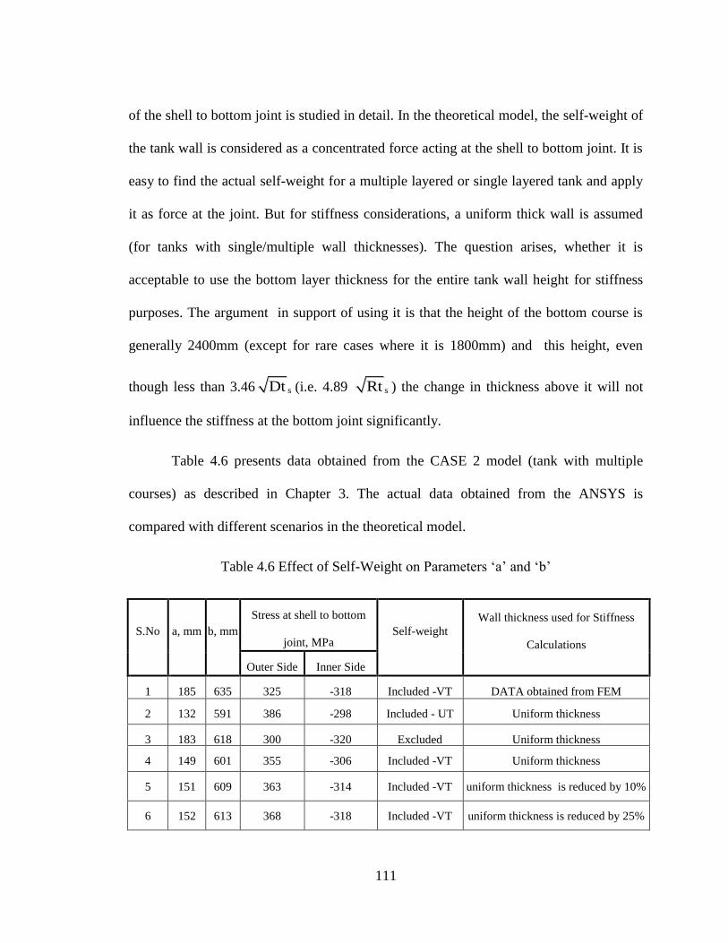
111
of the shell to bottom joint is studied in detail. In the theoretical model, the self-weight of
the tank wall is considered as a concentrated force acting at the shell to bottom joint. It is
easy to find the actual self-weight for a multiple layered or single layered tank and apply
it as force at the joint. But for stiffness considerations, a uniform thick wall is assumed
(for tanks with single/multiple wall thicknesses). The question arises, whether it is
acceptable to use the bottom layer thickness for the entire tank wall height for stiffness
purposes. The argument in support of using it is that the height of the bottom course is
generally 2400mm (except for rare cases where it is 1800mm) and this height, even
though less than 3.46 sDt (i.e. 4.89 sRt ) the change in thickness above it will not
influence the stiffness at the bottom joint significantly.
Table 4.6 presents data obtained from the CASE 2 model (tank with multiple
courses) as described in Chapter 3. The actual data obtained from the ANSYS is
compared with different scenarios in the theoretical model.
Table 4.6 Effect of Self-Weight on Parameters ‘a’ and ‘b’
S.No a, mm b, mm
Stress at shell to bottom
joint, MPa Self-weight
Wall thickness used for Stiffness
Calculations
Outer Side Inner Side
1 185 635 325 -318 Included -VT DATA obtained from FEM
2 132 591 386 -298 Included - UT Uniform thickness
3 183 618 300 -320 Excluded Uniform thickness
4 149 601 355 -306 Included -VT Uniform thickness
5 151 609 363 -314 Included -VT uniform thickness is reduced by 10%
6 152 613 368 -318 Included -VT uniform thickness is reduced by 25%

112
Notes:
VT: Variable Thickness, - the self-weight is calculated for the tank with
multiple layers
UT: Uniform Thickness - the self-weight is calculated for the tank assuming
that the entire height of tank wall has same thickness as that of the bottom layer
“uniform thickness” in the stiffness calculations indicate that the thickness of
the entire wall is assumed same as bottom layer thickness
From examining the data in Table 4.6, it can be seen that, for finding the required
projection length of the bottom plate and the corresponding stress values on either side of
the joint, excluding the self-weight and assuming the bottom layer thickness for the entire
wall for stiffness is appropriate. This assumption will give a slightly lower value of
bending stress on the outer side of joint. Since it is a location outside the tank, and
yielding and plastic hinge are allowed in this zone, this can be ignored. Similar to the
case with ambient temperature tanks, providing extra projection length in elevated
temperature tanks reduces the plate stress on the inner side of the shell to bottom joint
and increases the stresses on the outer side. Apart from the joint, the stresses are also
generally reduced in the inner portion of the bottom plate as shown in Fig. 4.15.

113
Fig. 4.15 Bending Stress in the Bottom Plate of Elevated Temperature Tank
The figure refers to a tank with 30m radius, 12m height, 18mm shell thickness
and 6mm bottom plate subjected to a uniform temperature rise of 347F (175C).
Axisymmetric shell elements are used to model the tank wall and bottom plate with
contact elements for bottom plate - subgrade interaction.
4.10 EFFECT OF SELF-WEIGHT ON STRESSES (COMPARISON
USING FEA)
This section discusses the effect of self-weight on the stresses in the tank wall and
bottom plate. A tank with multiple wall thicknesses (CASE 2 - described in Chapter 3) is
considered. It is a fairly big tank in the upper end of the design range. Two FE models
with and without the self-weight effect are used for the study
A

114
Fig. 4.16 Bending Stress in Bottom Plate (Bottom Side) – With and Without Self-weight
. Figures 4.16 and 4.17 show the bending stress in the bottom plate for three
different load factors (0.7, 1, and 1.4). “LF” indicates Load Factor; a value of 1 indicates
that the tank is filled fully with a liquid of specific gravity 1. Fig 4.17 is the same as
Fig.4.16 but zoomed and expanded near the shell-to-bottom joint.

115
Fig. 4.17 Bending Stress in Bottom Plate – With and Without Self wt. – Expanded View
Near Tank Wall
From the plots above it can be seen that the self-weight affects the bending stress
of the bottom plate only in a small portion on the outer side of the shell to bottom joint.
Inner side, the stresses are not significantly affected by the self-weight. For the LF=1
case, the maximum difference occurs close to the joint (3mm from the shell on the outer
side). The stresses increase from 133 MPa to 152 MPa with the inclusion of self-weight
effect (14.3% increase). For small tanks or for lower loads, it can be expected that the
percentage change will be much less. However, it should be noted that this zone is
outside the tank and yielding is permissible in this region. Hence ignoring the self-weight
may not have adverse effects.
Wall Thickness

116
Fig. 4.18 von Mises Stress in Shell Wall – With and Without Self-weight Consideration
Figure 4.18 shows the stresses in the tank wall. As expected, shell stresses are not
significantly affected by the self-weight. The maximum difference in stress for load case
LF=1 is only 3 MPa higher with self-weight. The zones marked as ‘D’ in the stress plot
for each load case are due to discontinuity resulting from change in tank wall thickness.
In case of openings at tank bottom, it can be qualitatively said that there will not
be uplift of the bottom plate directly below the opening and hence the projection length
determined using the proposed analysis will be conservative. However, the uplift length
may be larger near the edges of opening because of the extra moments transmitted from
the shell. This may cause the strains in the bottom plate to slightly increase on the inner
side. The nozzle loads may increase or decrease the corresponding bottom plate stresses
slightly based on the direction of the nozzle load.
D

117
4.11 CLOSURE
The shell to bottom joint is an important high stress location in the tank where the
material is close to yield or in plastic range. This joint is a critical failure zone for tank
failure. Hence proper evaluation of stresses in this zone is very important. Denham’s
beam model (where the projection length is assumed to be fixed as 3”) is reviewed and
validated using FEA. The model is extended to any arbitrary projection length. Using this
theoretical approach and FEA, the effect of bottom plate projection beyond the shell wall
has been studied for tanks on rigid ring wall foundations. It is found that the length of
projection changes the stresses in the shell as well as the bottom plate near the shell to
bottom joint. Increasing the length is beneficial. The stresses will not alter if the length is
increased beyond a certain limit, which is being termed as ‘full projection length’. An
extension to Denham’s model is proposed to determine this ‘full projection length’. The
theoretical results are validated using FEA. The effect of assuming a uniform thickness
for a variable thickness tank wall for the sake of determining the ‘full projection length’
is studied and found to be acceptable. Similarly the results of including or excluding the
self-weight of the tanks are compared. The self-weight of tank does not increase the
stresses in the tank wall or the bottom plate on the inner side of the shell to bottom joint,
whereas it may increase the stresses marginally on the outer side of the joint.
An expression for the tank wall bottom moment has been presented for ambient
temperature tanks. Using the expression the designer can readily find the moment at the
shell to bottom joint and hence the stresses in that zone. This equation is based on a fully
elastic model and may be used to find the stresses near the shell to bottom joint.

118
CHAPTER 5
INCORPORATION OF FRICTION COEFFICIENT IN
ELEVATED TEMPERATURE TANK DESIGN
Storage tanks operating at elevated temperatures (200F to 500F) need to
consider stresses due to thermal expansions and restraints to the expansion in addition to
the design requirements for ambient temperature tanks. Appendix M of API Standard 650
provides additional requirements and guidelines for the design of tanks operating at
elevated temperatures. These are based on Karcher’s method [Karcher, 1978a, b] which
gives a simplified procedure for determining the stresses in the tank wall and bottom
plate. During temperature cycle, the tank will expand radially at the bottom. This
expansion is partially or fully restrained by friction between the tank bottom and
foundation components. A factor named ‘C’ is used for defining the ratio of actual
expansion to free expansion of the tank. Such partial expansion causes significant thermal
stresses. API uses these stresses to estimate the low cycle fatigue life of the tanks. At
present, a range of ‘C’ values (0.25–1.0) is allowed by API without clear guidelines for
selecting a suitable value. If no other choice is available, API 650 specifies that ‘C’ be
taken as 0.85. API 650 does not provide any guidelines to determine the ‘C’ factor. The
present study is aimed at systematic estimation of the ‘C’ factor by relating it to the
friction coefficient. This Chapter evaluates the current procedure and suggests an

119
alternate method by incorporating the friction coefficient directly in the stress equations,
instead of the ‘C’ factor.
5.0 BACKGROUND
In many industries, storage tanks are needed to hold liquids like asphalt,
residuum, high pour point hydrocarbons, etc., at higher temperature than the ambient.
This gives rise to thermal stresses in the tank, especially near the shell-to-bottom joint.
The magnitude of thermal stress occurring in the tank wall and the bottom plate is
influenced by the amount of radial restraint, which in turn depends upon factors like
liquid pressure, friction between the bottom plate and the foundation, piping connections
and differential settlement. In addition, from low cycle fatigue point of view, the cyclic
loading due to continual filling and draw down is reported [Long and Garner, 2004] to be
more severe for elevated temperature tanks compared to that for ambient temperature
tanks.
The general basis of the tank wall design for tanks operating at ambient
temperature (any temperature less than 200F or 93C) is to limit the hoop stress to the
allowable limits using either the 1-Foot Method or the more accurate Variable-Design-
Point Method. American Petroleum Institute Standard, API 650 [2012] adopted these
design procedures which were originally proposed by Zick and McGrath [1986]. In the
case of elevated temperature tanks, API 650 provides guidelines in Appendix M
“Additional Requirements for Tanks Operating at Elevated Temperatures.” This gives
requirements for operation of large storage tanks at temperatures up to 500 F (260 C). It

120
is recommended that, for designing the tank wall, the same procedure as that of ambient
temperature tanks shall be used with modified allowable stress limits based on strength
reduction factors for the design temperature. This Appendix provides design
considerations for limiting the loadings and strains resulting from thermal effects, such as
differential thermal expansion, tank bottom plate buckling and thermal cycling.
A typical complete thermal cycle for an elevated temperature tank can be
described as follows [Jones and Seshadri, 1989]:
Gasoil is pumped in to the storage tank and then heated to a specified
temperature
The Gasoil is heated slowly to allow any excess water to be removed by
drainage or blow off. This step will also allow gradual thermal expansion of the tank
and shell
The tank is filled with a high pour point hydrocarbon. When there is a demand
for stored fluid, the tank is drawn down to a specified level and the procedure is
repeated as needed.
For tanks with maximum design temperature greater than 93C (200°F), particular
consideration should be given to the following thermal effects [API 650]:
Temperature differences between the tank bottom and the lower portion of the
shell. Such thermal differences may result from factors such as the method and
sequence of filling and heating or cooling, the degree of internal circulation, and
heat losses to the foundation and from the shell to the atmosphere. With such

121
temperature differences, it may be necessary to provide for increased piping
flexibility, an improved bottom-to-shell joint, and a thicker annular ring or bottom
sketch plates to compensate for increased rotation of the bottom-to-shell joint.
The ability of the bottom to expand thermally, which may be limited by the
method of filling and heating. With such a condition, it may be necessary to
provide improved bottom welding in addition to the details suggested above.
Temperature differences or gradients between members, such as the shell and
the roof or stairways, the shell and stiffeners, the roof or shell and the roof
supports, and locations with insulation discontinuities.
Whether or not the contents are allowed to solidify and are later reheated to a
liquid, including the effect on columns, beams, and rafters. The possible build-up
of solids on these components and the potential for plugging of the vent system
should also be considered.
The number and magnitude of temperature cycles the tank is expected to
undergo during its design life.
The shell-to-bottom joint is a critical location vulnerable in many modes of
failure. Denham, et al. [1968a, b], Wu and Liu [2000] and Sathyanarayanan and Adluri
[2011] have proposed methods to determine the stresses in the bottom plate near this joint
for ambient temperature tanks. As mentioned above, this joint is subjected to low cycle
fatigue due to cyclic loading of the stored liquid (fill–draw down cycle) or the fluctuation
in the temperature of the stored liquid or both. Karcher [1978a, 1978 b, 1981a, 1981b]
carried out a ground breaking and very useful study on elevated temperature tanks. He

122
provided stress equations based on an assumed plastic hinge boundary condition at the
shell-to-bottom joint. Based on these, he proposed a simplified procedure to find the
fatigue design life of the tank considering the maximum stress developed at the shell-to-
bottom joint and a relevant stress concentration factor. API 650 has adopted Karcher’s
procedure for determining the design cyclic life of the tank.
5.1 CURRENT PRACTICE
The current practice assumes uniform temperature increase in the tank, i.e.,
without any temperature gradient across the thickness of the shell wall. This is a
reasonable assumption since the shell wall thickness is relatively thin and carbon steel is
a conductive material. At steady state, the difference in temperature should not be
significant. In addition to these, the temperature difference (if any) between the bottom
region of the shell and the bottom plate that might be caused by heat loss is ignored. The
stresses are determined using shell theory for tank wall while beam-on-elastic foundation
theory is used for the bottom plate. It is assumed that complete plastic hinges are formed
in the bottom plate near the shell-to-bottom joint [Karcher 1978 a, 1978b, 1981a, 1981b],
while the shell stresses are assumed to be elastic. Essentially the equations as given by
Timoshenko and Woinowsky-Kreiger [1959] for cylindrical tanks with clamped end
conditions are suitably modified to have the plastic moment at the bottom as the
boundary condition. The hydrostatic stresses caused by liquid infill are combined with
the stresses that may be induced due to heating of the filled liquid. Two plastic hinges are

123
assumed at the bottom plate for a rigid foundation (such as concrete ring wall or pile cap)
while one hinge is used for flexible subgrade below the tank wall.
5.1.1 Stresses in Shell (Tank Wall)
Based on the shell theory [Timoshenko and Woinowsky-Kreiger, 1959], the
following equations were given by Karcher [1981a, b] with an assumption of a single
plastic hinge at the shell bottom (applicable for the earthen foundation case),
The radial deflection of the tank wall (ys) is given by
s
22xs s o
s s s s
s
TEt C TEt 2 MRy H x e H cos x sin x
Et R R
(5.1)
where, is the coefficient of thermal expansion, T is the uniform temperature rise, C is
the reduction factor for T to account for the friction restraint, Mo is the moment at the
shell to bottom joint and ‘xs’ is the height of a point along the tank wall at which the
deflection is calculated.
The bending moment, hoop force and shear force of the tank wall at a distance
‘xs’ from the tank bottom are given by
s
s
2x s o
x s s2
C TEt 2 MM e H sin x cos x
R2
(5.2)
s
2x s o
s s s
C TEt 2 MN R H x e H cos x sin x
R
(5.3)
s
s
2x s o
x s s s s
C TEt 2 MQ e H cos x sin x sin x cos x
2 R
(5.4)

124
If T in the equations above is assumed to be zero, then these equations reduce to
those for a cylindrical shell loaded by hydrostatic pressure as given by Timoshenko and
Woinowsky-Kreiger [1959]. These equations can be used to find maximum stress
intensities in the shell and hence fatigue evaluation can be carried out, if required, for the
loading cycles that are expected during the design life of the tank.
All the above equations were developed based on the assumption that the boundary
condition at the shell to bottom joint is represented by a moment Mo and zero radial
deflection. Both of these assumptions (with Mo replaced by a single plastic hinge) were
first used by Zick and McGrath [1968] for finding the stresses in the shell wall for an
ambient temperature tank. The basis of these assumptions is given in their report to the
API. The validity of the first assumption will be discussed in Chapter 6. Regarding the
second assumption, Karcher [1978a, 1978 b] explains that even though the assumption of
zero deflection seems to be open to question, in actual practice, an elevated temperature
tank is usually filled initially to a level of several meters with only partially heated or
cold product. Then internal heaters and mixers are used to increase and maintain product
temperature. This start up procedure (with a smaller liquid head being heated to full
temperature) results in the tank bottom expanding more freely than the case where the
full liquid head is heated from ambient temperature. This results in lower frictional
resistance between tank bottom and the foundation. Preliminary observations on several
tanks indicate that the annular plate expands radially by about one half of the calculated
value of RT. Therefore assuming that the annular plate expansion is between zero and

125
half of RT is a reasonable approximation with the former being more conservative
[Karcher, 1981a].
Karcher accounted for the partial radial expansion of bottom plate by employing a
reduction factor (‘C’) in the equations above. A ‘C’ value of 1 assumes a fully restrained
bottom to shell junction (0% radial expansion) and a value of zero assumes free (100%)
radial expansion. The bottom will have free expansion (equal to RT) if there is
essentially no friction. But in reality, there are friction forces under the tank
bottom/annular plate (including backing plates, etc.) and hence the plate expands partially
(0.25≤C≤1.0). The magnitude of friction forces also depends on the liquid head in the
tank available at the time of heating.
5.1.2 Stresses in Annular Plate
The shell-to-bottom joint location is a region of high strains and plastic hinges are
assumed to form in the bottom plate near this location. The stress created here can be
classified as secondary bending stress and hence should be limited to twice the yield
strength of the annular plate material to assure shakedown to an elastic action. The
pseudo bending stress representing the strain range that occurs in the tank annular plate at
the shell-to-bottom joint is obtained by the following procedure [Karcher, 1978a]:
From Eq. 5.1, assuming a fully plastic annular plate moment at the shell bottom
(i.e., Mo = Mp), the slope at the bottom of the tank wall is determined as
3 22
0
1- -2
s
s s Y bS
s sx
dy C TEt S tRH
dx Et R
(5.5)

126
In order to find the strain range in the annular plate at the shell-to-bottom
junction, it is assumed that annular plate reacts like a beam-on-elastic foundation.
Following Hetenyi [1971], the moment in the plate is M = K/43, where, Ω = 4
3
3
bEt
K
and K is the modulus of the subgrade.
The value of slope as obtained from Eq. 5.5 is used in M = K/43 resulting in
γ
tSβ
γR
TEtCαH
E
Kt
t
RS bYsb
sb
21
658.023
4
2
(5.6)
where, Sb is the pseudo bending stress representing the strain range at the bottom
plate
Equation 5.6 is valid only if the following condition is true.
2
23bYs tSβ
R
TEtCαH
(5.7)
This condition ensures that the tank is loaded thermally or hydrostatically such that a
single plastic hinge forms in the bottom plate near the shell-to-bottom joint. The safe
design cycle life, N, is given by,
44.29700
SKN
c (5.8)

127
where, S is the alternating stress range in MPa (=Sb/2), Kc is the stress concentration
factor. This procedure to ensure the safe cyclic life of tank can be avoided if a significant
head of heated liquid (close to design temperature) is maintained in the tank between
cycles. A significant liquid head can be defined as being equal to or greater than
0.4(Dts)0.5
ft, where, diameter D is in feet and ts is in inches [API 650].
Fig. 5.1 Meridional Moment in the tank [Karcher, 1978a]
Figures 5.1 and 5.2 demonstrate the effect of temperature rise on moments and
equivalent stresses (strain range) in the tank wall and the bottom plate. The results show
that these stresses can be significant on the lower shell courses and annular plate regions
close to shell bottom. Equations 5.5 – 5.8 depends on the C factor and hence using a
proper C value becomes important.

128
Fig. 5.2 Annular Plate Bending Stress Caused by Hydrostatic and Thermal Loads
[Karcher, 1978a]
Equations 5.1-5.4 are valid for ambient and elevated temperature tanks. The basic
assumptions involved in these equations regarding radial growth characteristics and the
bottom moment of the tank wall have significant influence on the stresses in the tank
wall. Regarding the radial deformation, as mentioned earlier, it is obvious that bottom
plate can expand anywhere between zero to full radial growth (RT). No guidelines for
selecting the actual value (within the allowable range) are available either from API or
other sources. Although the current practice has not been publicly reported to have
resulted in field failures and hence can be construed to be safe, use of a set value of C for
all situations is not appropriate as discussed later in the Chapter. An equivalent but
considerably less problematic approach using friction coefficient is discussed below.

129
5.2 INCORPORATION OF FRICTION COEFFICIENT IN DESIGN
EXPRESSIONS
If the tank foundation does not restrain the expansion due to temperature (at least
partially), then the thermal stresses will be minimal. However the foundation generally
offers significant frictional resistance that restrict the free radial expansion of elevated
temperature tanks which in turn induces additional thermal stresses in the tank wall. The
following model obtains the partial radial expansion by first finding the effective
contraction due to the friction forces and subtracting it from the free thermal expansion.
The treatment is similar to that of a disc subjected to centrifugal forces. Considering the
equilibrium of an infinitesimal element in the bottom plate of the tank as shown in Fig.
5.3 (a).
Hdrdrtdrd
tdrtddrrd pprrprrrr
22)( (5.9)
where, σrr and σ are the stress components in the radial and circumferential directions,
is the coefficient of friction between the bottom plate and the foundation as appropriate
to the given conditions. It is generally assumed that the tank bottom is resting on well
compacted dry sand/gravel. The equation assumes that the friction forces are
predominantly in the membrane direction of the bottom plate [Sathyanarayanan and
Adluri, 2013c].
Neglecting higher order terms in Eq.5.9,
p
rrrr
t
H
rdr
d
1 (5.10)

130
Fig. 5.3 Friction Forces Below Bottom Plate
For axisymmetric plates the stress displacement relationships are given by [Boresi and
Schmidt, 1993]
Tank wall
Mo
Hydrostatic
Pressure
Bottom
Plate
R
r
dr
d
σrr + d σrr
(b) σ
σ
σrr
(c)
(a)
xs
Friction Forces Annular Plate
Qo H Tank weight

131
r
u
dr
duErr
21 (5.11)
r
u
dr
duE
21
(5.12)
where, u is the radial displacement at any point in the bottom plate due to friction forces.
The negative sign in Eq. 5.10 indicates the contraction of the plate.
Substituting (5.11) and (5.12) in (5.10)
pt
H
r
u
dr
du
rdr
udE
22
2
2
1
1 (5.13)
Solving Eq.5.13,
2 2
2
1
1
3p
H r Cu C r
E t r
where, C1 and C2 are constants of integration. Using appropriate boundary conditions for
the given loading,
2
3
1r
t
H
Eu
p
(5.14)
It must be pointed out that in addition to the above, there will be other effects
due to shear at the bottom, self-weight of bottom plate and tank wall stiffness (in relation
to that of the bottom plate). These can be shown [Adluri, 2012] to have only a small
influence. Other effects such as those due to local loss of contact with the foundation,
local bending of bottom plate due to bulging (or buckling), bottom plate lap welds, weld

132
reinforcements, backing strips, horizontal soil pressure due to uneven bottom surface of
the plate, etc., have also been omitted in the present treatment. Although the bottom plate
is treated with a single thickness here, multiple thickness plate along with other effects
omitted above can be incorporated. In a recent report, Adluri [2012] extended the
treatment given in the present chapter and discussed these issues at length along with the
effects of non-uniform friction below the bottom due to soil shearing under parts of the
bottom plate. The treatment in the present thesis is a general approach that can be used
with a single equivalent value for for the entire bottom plate.
Hence for any tank subjected to uniform temperature increase T, the partial
radial expansion of the tank bottom after filling the liquid to a height H and heating it to
the required temperature, will be given by
pt
RH
ETR
2
3
1
(5.15)
Note that H indicates the actual liquid height and not the constructed height of the tank
wall. The ‘C’ factor as used currently can be interpreted to represent the ratio between
the restraint deformation due to friction forces and the free expansion of the bottom plate.
Hence,
Tt
RH
EC
p
3
1 (5.16)

133
The ‘C’ value will be 1.0 when the restraint deformation as calculated is equal to or more
than the free thermal expansion. The C-factor will be zero if the restraint deformation is
zero.
5.2.1 Incorporation of Friction Coefficient in Shell Equations
The governing equation for circular cylindrical shell (Fig.5.4) loaded
symmetrically with respect to its axis [Timoshenko and Woinowsky-Kreiger, 1959] is as
follows
44
44s
sss
d y wy
Ddx (5.17)
where, ys is the radial deflection, w is the liquid pressure acting inside the cylinder, β and
Ds are shell parameters, where
3
212 1
ss
EtD
The general solution for the above equation is
1 2 3 4cos sin cos sin ( )sx xs s s s s sy e c x c x e c x c x f x
(5.18)
For circular tanks with uniform wall thickness, Eq. 5.17 is modified as
(5.19)
A particular solution of Eq.5.19 is
2s
ss
H x Ry
Et
(5.20)
The complete solution of Eq. 5.19 is
2
1 2 3 4cos sin cos sins s sx xs s s s s
s
H x Ry e c x c x e c x c x
Et
(5.21)
44
44
sss
ss
H xd yy
Ddx

134
Considering the shell as infinitely long; c1 = c2 = 0
Fig. 5.4 Forces in Tank
Using the boundary condition that there is no radial expansion at the bottom of the
tank (for hydraulic loading only) and the moment at the tank bottom is Mo, Eq. 5.22 is
obtained. The moment (Mo) at the tank bottom can be a maximum of one/two times the
plastic moment capacity of the bottom plate. It is denoted by Mb.
In case of earthen foundation, with a single plastic hinge on the
inside
2
4
y pb
S tM and in case of concrete ring wall foundation, with a plastic hinge on
either side of shell
2
2
y pb
S tM . This gives,
(5.22)
22
2cos sin
2
s sx bs s s
s ss
H x RMHRy e x x
Et EtD
ys (outward
positive)
R
H
xs
Mo
w
Qo

135
(5.23)
…….. (5.24)
5.2.2 Thermal Stresses in Cylinders
Fig. 5.5 Schematic Expansion of Tank
In Fig. 5.5, δ is the free expansion of cylinder for a uniform temperature increase
of T. If friction is present, δ is the expansion at the bottom of the cylinder (and the
bottom plate) for a uniform temperature increase. From Eq.5.17 & 5.18 and considering
the shell as infinitely long with only temperature loading, Eq.5.25 can be obtained. The
term f(xs) representing the particular solution in Eq.5.18 becomes zero since there is no
pressure loading for pure temperature loading (which can be added to the separate
solution obtained for hydrostatic loading).
2 2
2cos sin cos sin
2
sxs bs s s s
s s ss
dy M HR Re x x x x
dx Et EtD
2 22
2 22 sin cos
2
sxs bs s
ss s
d y MHRe x x
Etdx D
δ = RT
(b) Thermal Expansion of Tank with
Frictional Forces
(a) Free Radial Expansion of Tank
under Temperature Change
QT
δ = 21
3p
H r
E t
QT
MT MT
δ = RT

136
3 4cos sinsxs s sy e c x c x
2
23 42
2 sin cossxss s
s
d ye c x c x
dx
3
33 3 4 43
2 cos sin sin cossxss s s s
s
d ye c x c x c x c x
dx
(5.25)
. (5.26)
... (5.27)
… (5.28)
Let MT and QT be the moment and shear force induced at the bottom due to thermal
loading,
2
20ss
sx s T
xs
d yM D M
dx
(5.29)
3
300 0
s
ss
s
x sx s
xs sx x
dM d yQ D
dx dx
(5.30)
From Eq. 5.29 and Eq. 5.27
4 22
T
s
Mc
D (5.31)
From Eq. 5.30 and Eq. 5.28
3 3
1
2t T
s
c Q MD
(5.32)
Substituting the constants,
-4 3cos -sin - cos sinsxs
s s s ss
dye c x x c x x
dx

137
-
cos -sin - cos sin2
sxs T T
T s s s ss s
dy Q MeM x x x x
dx D
- 2
2
1cos -sin - cos sin
32
sxs Ts s s s
s ps
dy Me x x R H x x
dx t ED
2- 2 2
2 2
12 sin cos
3 2
sxs Ts s
ps s
d y Me R H x x
t Edx D
3 2
cos sin2 2
ss xxT
s T T s s
s s
e Mey Q M x x
D D
(5.33)
(5.34)
Considering the boundary condition as shown in Fig. 5.5 (b),
2
0
1
3ss xp
y R Ht E
(5.35)
Equating Eq. 5.33 and Eq. 5.35 at xs = 0
2
3
11
32T T
p
Q M R Ht ED
(5.36)
Using Eq. 5.36 in Eq. 5.33
2
2
1cos sin
3 2
ss
xx T
s s sp s
e My e R H x x
t E D
(5.37)
(5.38)
(5.39)
Using the principle of superposition, displacement (w), moment (Mx) and shear
(Qx) due to the liquid infill and the temperature rise is given by
22
2
11cos sin
3 2
s T b sxs s s
s p ss
M M H x RR Hy e x x
t t E E tD
(5.40)

138
2 2
2
cos sin2
11cos sin
3
s
T bs s
sβxs
s ss s
s p
M Mx x
Ddy R e
dx E tR Hx x
t t E
..(5.41)
222
2 2
cos2
211
sin3
s
s
T bs
sβxsx s s
ss
s p
M Mx
Dd yM D D e
dx R Hx
t t E
(5.42)
2
33
3
2
11cos sin
32
sin cos2
s
s
s ss pβxs
x s s
s T bs s
s
R Hx x
t t Ed yQ D D e
dx M Mx x
D
(5.43)
2
2
11cos
3
sin2
ssβx
s pss
T bs
s
R Hx
t t Ee EtN H x R
R M Mx
D
(5.44)
where, MT and Mb represent the moment induced at the bottom due to thermal and
hydrostatic loadings. The sum of these moments cannot exceed 2Mp for rigid foundations
and Mp for flexible foundations. These equations (Eq. 5.40- 5.44) are similar to Eq. 5.1 -
5.4, where, C is replaced with the expression from Eq. 5.16. Equations 5.40 – 5.44 are
valid only if ‘δ’ from Eq.5.15 is greater than zero i.e. the thermal expansion of bottom
plate is not less than the restraint offered by the frictional forces at the tank bottom. If this
is not so, it implies that the bottom of the tank does not expand at all because of high

139
amount of frictional resistance. For this case, replace the term (1-)/3tp with ET/RH
in the eq. 5.40-5.44.
With respect to stresses in the tank wall, Karcher’s equations will yield the same
results as those of the proposed model provided an exact C-factor is used. The value of
‘C’ has a significant influence on tank wall stresses. Predicting this factor during the
design stage or even during operation without any field measurements is a difficult task.
Hence using standard friction coefficients between known materials and determining the
stresses using Eq. 5.40 - 5.44 will be an appropriate choice.
5.3 RESULTS AND DISCUSSION
Finite element analyzes were carried out using ANSYS to explore the effect of
friction and validate the theory above. The foundation is assumed to be a concrete ring
wall with highly compacted infill. Axisymmetric SHELL elements were used for
modeling the tank wall and bottom plate. Both elastic and elastic-perfectly plastic
material models were used as described in Chapter3.
The example tank (CASE 1) from Chapter3 with T = 347F (175C) and = 0.3
is considered for the study. Figure 5.6 shows theoretical deflection in tank wall with a
double hinge condition for bottom plate as specified by Zick and McGrath [1968] and
Karcher [1978 a,b,1981 a,b]. The shell stresses from nonlinear FEA (which does not rely
on the double hinge assumption) match well with theoretical stresses. This implicitly

140
confirms the formation of two plastic hinges in the bottom plate near shell bottom in the
FE model. The bending and hoop stresses for this analysis are shown in Figs.5.7 and 5.8.
It is to be noted that eventhough the bottom plate can reach plastic stage, the shell
stresses are designed to be within elastic limits for operational loads.
Fig. 5.6 Deflection in the Tank Wall Including the Effect of Friction (=0.3)

141
Fig. 5.7 Bending Stress (Sx) in Tank Wall Including Friction Effects (=0.3)
Fig. 5.8 Hoop Stress in Tank Wall Including Friction Effects (=0.3)

142
The same tank with = 0.5 is analyzed using elastic-plastic FE model. Figure 5.9
compares the FEA results and the theoretical values. The theoretical radial displacement
(horizontal movement) at the outer edge of the annular plate (Eq. 5.15) is 52.7 mm. The
corresponding radial displacement as obtained from FEA (including friction effects) is
53.4 mm. If there were no friction forces, the expansion would be RT=63mm (with
=12x106). For this example the value of C can be calculated as 0.15 (=[63-53.4]/63). It
can be seen that this value is far smaller than the value of 0.85 recommended by API 650.
Even though, the analysis indicates that two plastic hinges form at the bottom
plate for this case, a complete double hinge may not always form at the bottom for
general tanks. For the tank considered, two full hinges will not form if either the friction
coefficient or the temperature is less than the values used above. Hence using two plastic
hinges as boundary condition for lower temperature tanks or those with smaller friction
coefficient will underestimate the maximum stresses in the tank wall.

143
Fig. 5.9 Bending Stress in the Tank Wall Including Friction Effects – (Elastic-Plastic
FEA)
Hoop and Bending stress values are obtained for a tank with the same dimensions
as before but with different values of and C. The comparisons are shown in Fig. 5.10
and 5.11. From the figures it can be seen that the bending stress in tank wall for even a
friction coefficient as high as 1.0 is considerably less than the stress obtained using a C
value of 0.5. Hoop stress in the tank wall also shows a similar trend. Hence for the
example tank dimensions, using a C-factor of more than 0.5 is excessively conservative.
115 MPa

144
Fig. 5.10 Tank Wall Bending Stress for Various Values of ‘C’ and
Fig. 5.11 Tank Wall Hoop Stress for Various Values of ‘C’ and

145
For a value of in the range 0.30.5 the difference will be even more
pronounced. Figure 5.12 shows the variation of shell stresses as temperature increases
with friction being constant (for a friction coefficient of = 0.7).
Fig. 5.12 Tank Wall Bending Stress at Different Temperatures for = 0.7
For a given tank, the bending stress caused by friction will be maximum when
u=RT or C =1. Hence from Eq. 5.14, for a particular friction coefficient
1
3L
p
H RT
E t
(5.45)
where, TL is the limiting temperature beyond which increase in temperature will not
increase the stresses. Conversely, the limiting friction coefficient can also be obtained as
below.

146
3
1
pL
T tE
H R
(5.46)
where, L is the friction coefficient that will cause maximum stresses for a particular
temperature. If a friction coefficient value is chosen higher than L, there will be no
further increase in the stresses. In other words, this is the ‘’ at which the C becomes 1.
For any greater than this value, C continues to be 1 as it represents zero expansion
condition.
For the example tank used earlier, TL is 40C, it can be seen from Fig. 5.12 that
the stresses (from FEA) in the tank wall do not increase when the temperature is
increased beyond this limit. Basically, if the restraint deformation due to friction is equal
to or greater than the free radial expansion due to temperature, the stresses in the tank
wall will reach a maximum and further increase in temperature does not have any impact.
For the same tank as above but with a friction coefficient of 0.7, the C-factor
changes with temperature as shown in Fig. 5.13. The plot indicates that C value is 1.0 till
the temperature is 40C, which is the temperature limit TL for this tank. The stresses in
the tank bottom increase till the temperature reaches the limit TL and remain constant
after this limit. Hence after TL, the C value reduces inversely with temperature such
that the state of stress at TL is maintained throughout. It should be noted that though C
value reduces, the product of T and C will remain constant. This is a unique value for
each tank and is directly proportional to the friction coefficient. The pattern for C-factor
as shown in Fig. 5.13 holds good for any typical tank. The tank dimensions will only alter

147
the value of TL limit. This observation implies that the present recommendation of
C=0.85 [API 650] for any tank may or may not be conservative (although no failures are
reported to the best of the author’s knowledge in general literature). If the temperature is
relatively low and the friction coefficient of the tank is high, then its C value could
sometimes be in the region A-B of Fig. 5.13 (before TL limit) and hence C = 1. For this
case, using C < 1 is unconservative. On the other hand, stresses predicted using C = 0.85
for temperatures at the end of region B-C will be very highly conservative.
Fig. 5.13 Temperature Influence on C-Factor
Using a flat value for the C-factor (be it 0.5 or 0.85) gives inconsistent results. At
present there are no clear guidelines on choosing a value of C other than 0.85. The
margin of safety varies with operating temperature and could result in slightly
unconservative estimates temperature ranges less than TL and grossly conservative
predictions at higher temperatures. This is further illustrated in Table 5.1 which shows
C = 0.85

148
the implied coefficient of friction for fixed values of C equal to 0.5 and 0.85 for typical
elevated temperature tanks.
Table 5.1 Implied Coefficient of Friction for Fixed Values of C-Factor
H D tb T Implied
m m mm oC
C =
0.5
11 16 6 93 3.32
11 16 6 260 9.29
11 90 7 93 0.69
11 90 7 260 1.93
19.2 16 8 93 2.54
19.2 16 8 260 7.10
19.2 61 8 93 0.67
19.2 61 8 260 1.86
C =
0.8
5
11 16 6 90 5.47
11 16 6 250 15.19
11 90 7 90 1.13
11 90 7 250 3.15
19.2 16 8 90 4.18
19.2 16 8 250 11.60
19.2 61 9 90 1.23
19.2 90 11 90 1.02
19.2 61 9 250 3.42
The implied coefficient of friction in Table 5.1 is calculated using Eq. 5.16. As
can be seen, except for very large tanks at relatively low temperatures, the implied values
of are unacceptable if the C-factor is fixed as 0.5. It is reported that C = 0.5 was based
on anecdotal observations on some tanks [Karcher, 1978a]. No Data regarding those
tanks is available. It is possible that they were very large tanks at temperatures in the 200
- 250F range. For these tanks, a C-factor of 0.5 may sometimes be acceptable. However,

149
as can be seen from the table, for other ranges of H, R and T, the implied values of
(for C = 0.5) are too high. API 650 recommends a value of C = 0.85 in case other
information is not available. This is generally assumed to be a conservative
recommendation. However for most tanks, the implied values of for this value of C are
even larger than those for C=0.5. Acceptable vales of are implied only for large
diameter tanks with low temperatures. Therefore, instead of using a seemingly
conservative value for the C-factor, it may be preferable to use a conservative estimate
for the friction coefficient . The actual value depends upon the type of subgrade and
can be obtained from established literature or other means. Adluri [2012] provided
extensive discussion on this issue.
It should also be understood that friction resistance depends on liquid heights,
foundation and bottom plate/annular plate characteristics. The value of the friction
coefficient is not likely to alter significantly within the temperature range being
considered (unlike the change in yield strength based on temperature change as given in
Table M-1 of API 650). Because of this, thermal effects do not necessarily increase
linearly with temperature. The extraordinary values for implied in Table 5.1 can be
understood by examining Eq. 5.15. Free thermal expansion is proportional to R and T
whereas the restraining displacement due to friction is proportional to R2 and H (and does
not depend significantly on T).
For smaller tanks in the Table, the friction resistance is not sufficient to provide
appreciable restraint against thermal expansion. As liquid height increases, friction

150
resistance proportionately increases while free thermal expansion (RT) stays the same.
When the radius increases, this effect is compounded. Hence as the tank size increases in
radius and height, the total friction force builds up and the restraining displacement starts
to approach the free thermal expansion. The opposite happens with increasing
temperature. These points can be further illustrated through Table 5.2 which lists the
implied C-factor for a fixed value of = 0.85. For smaller tanks, the implied C-factor is
quite small. Only for large tanks with relatively low temperature increase, the implied
C-factor approaches the values currently being used. At the outer edge of the range of
parameters, the implied C-factor can become slightly unconservative if a lower C value is
chosen for design. Hence, it is more rational to choose a conservative estimate for the
coefficient of friction than for the C-factor.
Table 5.2 Implied C-Factor for Fixed Values of Coefficient of Friction
H D tb T Implied
m m mm oC C-factor
=
0.8
5
11 16 6 90 0.13
11 16 6 250 0.05
11 90 7 90 0.64
11 90 7 250 0.23
19.2 16 8 90 0.17
19.2 16 8 250 0.06
19.2 61 9 90 0.59
19.2 90 11 90 0.71
19.2 61 9 250 0.21

151
5.3.1 Influence of Friction on Fatigue Life
In the current practice, the alternating stress required for fatigue life estimation of
tank (number of fill/draw cycles the tank can safely withstand) is determined by Eq. 5.6.
In this equation, the friction forces are indirectly represented by the C-factor. For the tank
example considered earlier, Fig. 5.14 shows the influence of C-factor on the fatigue life
of the tank (for T = 175C). The fatigue life reduces drastically if the C-factor is
increased.
Fig. 5.14 Influence of C-Factor on Fatigue Life
As per API 650, the tank has to safely withstand at least 1300 fill/draw cycles. If C is
assumed to be 0.85 (and K=2) as recommended by the API, the tank fails by a significant
margin (N=369). If the same tank is considered with a (most likely conservative) friction
coefficient estimate, say, 0.85, the number of design life cycles (N) that the tank can
1300 cycles

152
withstand becomes 1896 (which is well above the required limit). This is a case where the
API recommendation is overly conservative. If the tank is larger and is operating at
temperatures below 100 oC, using a smaller C value could sometimes be slightly
unconservative.
5.3.2 Influence of Filling Procedure
API 650 recognises (in Clause M.4.2) that the tank filling procedure influences
the amount of radial expansion and hence the stresses and fatigue life. Generally if the
tank is initially filled to a low height (at least 0.3(Dt)0.5
, where, D is in ft and t is in
inches, [API 650] and heated to the required temperature as a first step, the tank will
radially expand almost to its full expansion and hence the thermal shell stresses induced
will not be very significant. However it must be noted that it may be difficult to guarantee
that this will always be followed when the tank is likely to be in operation for many
decades. On the other hand if the tank is heated with a significant liquid head, it induces
thermal stresses due to the friction forces. These stresses have been explored throughout
the paper. In order to verify the API recommendation of preheating the tank with low
liquid head, a finite element analysis was carried out. Using Eq. 5.15 for the example
tank used in finite element analysis, the radial expansion is 62 mm for a 2 m liquid head
heated to 175C. FEA results give 62.2 mm confirming the theoretical prediction. The
corresponding free expansion (RT) is 63 mm (with =12x106). The results show that
with very low liquid head, the radial expansion of the bottom is almost the same as that of
free radial expansion. The stresses for this analysis are very close to those of the same

153
tank at ambient temperature thus indicating that the thermal stresses can be neglected if
the above procedure for liquid filling and heating is used.
5.4 CONCLUSIONS
This present study examines the influence of bottom plate friction forces on the
stresses in the wall of elevated temperature tanks. Karcher’s equations used for finding
the stresses in the tank wall are verified using a finite element model with contact
elements. The equations use a value called as C-factor to include the effect of partial
expansion due to temperature change. It is observed that the equations give correct results
if the exact C-factor is used. Since the C-factor is highly sensitive in influencing the tank
wall stresses, the designer needs expertise and judgement in deciding on the factor during
the design stage. The current practice does not have clear guidelines for selecting a C
value. In the absence of such guidelines, a set value (like 0.85) for the C-factor is being
used irrespective of the tank dimensions and temperature change. The present study
shows that this approach is grossly conservative for most of the range of design
parameters (H, R & T). On the other hand, for very large tanks at relatively low
temperature changes, this could become slightly unconservative. This study shows that
the C-factor is directly related to the friction coefficient () and tank parameters.
Appropriate equations for stresses and by extension, fatigue life are presented. It is shown
that for a given tank with a particular friction coefficient, there is a limiting temperature
(TL) beyond which any further increase in temperature will not increase the tank wall

154
stresses. Similarly for a given temperature increase in a tank, the stresses will not increase
further even if the friction coefficient is higher than a particular value (L). Several
related issues are discussed. The results are verified using finite element analysis
incorporating friction forces through contact elements between foundation and tank
bottom plate. The study shows that it is much more rational to use a conservative
estimate for the coefficient of friction than for the C-factor.

155
CHAPTER 6
FATIGUE ANALYSIS OF SHELL TO BOTTOM JOINT OF
TANKS
Shell to bottom joint of hydrocarbon storage tanks is a critical failure location
which needs careful evaluation especially in the case of elevated temperature tanks. The
fill/draw down cycle of the stored liquid causes low cycle fatigue near this joint and
hence a fatigue evaluation is recommended as explained in previous Chapters. The peak
alternating stress at this location, used to enter the fatigue curves is currently determined
using a pseudo elastic stress that represents strain range due to inelastic deformations. For
this, API 650 employs beam-on-elastic foundation theory. This theory is being used for
tanks resting fully on earthen foundation as well as those on concrete ring wall. This
Chapter studies the validity of using this theory for tanks with concrete ring wall
foundation which are much more rigid compared to earthen foundations. Some of the
difficulties in the current practice are highlighted. An alternative to the current model is
proposed to determine the peak stress at the shell to bottom joint of tanks resting on
concrete ring wall. The results are validated using finite element analysis.

156
6.0 INTRODUCTION
The shell (tank wall) to bottom joint of storage tank is subjected to low cycle
fatigue due to fill/draw down cycle and the temperature fluctuation of the stored liquid.
The storage tank standards API 650 and 653 consider this aspect in detail and provide
guidelines for determining the safe cyclic life of the tank based on the fatigue analysis of
this joint.
For the elevated temperature tanks, API 650 provides guidelines to determine the
appropriate thicknesses of structural members and determine the design cycle life of the
tank (based on the fatigue evaluation of the shell to bottom joint). As per API 650, it is
expected that the tank withstands at least 1300 load cycles in its lifetime. In Appendix M
of API 650, the peak alternating stress to be used for fatigue analysis of this joint is
determined using the original work by Karcher [1978, 1981 a, b]. He proposed a set of
design equations to determine the tank wall stress and the fatigue life of elevated
temperature tanks as given in Chapter 5. Jones and Seshadri [1989] studied the validity of
Karcher’s model using elastic finite element analysis of the shell with an assumed hinge
condition at the bottom.
In the current practice, the bottom plate is analyzed using beam-on-elastic
foundation theory. The resulting equations were derived basically for tanks on earthen
foundation by Karcher [1981a]. The same are applied to concrete ring wall foundations
except that two plastic hinges are assumed in the bottom plate (or annular plate) instead
of one plastic hinge in the case of earthen foundation. However, it must be noted that the

157
bottom plate resting on concrete wall loses contact in the immediate vicinity of the inside
face of the tank wall. This was recognized by the previous research works [Denham,
1968; Wu, 2000; Sathyanarayanan and Adluri, 2011] as well as the seminal work by Zick
and McGrath [1968]. The uplift, although small, is sufficient to cause clear separation of
bottom plate from the top of the concrete ring wall on the inside. Hence the stresses in
this region are not directly governed by beam-on-elastic foundation model.
6.1 FATIGUE AT SHELL TO BOTTOM JOINT
Figure 6.1 shows the rotation of shell to bottom joint of a tank resting on a rigid
base. As explained in Chapter 4, this rotation causes the bottom plate to lift off the
ground over a small distance (say, uplift length L). Beyond this, the downward liquid
pressure acting on the plate is sufficient to make the plate fully rest on the foundation.
Fig. 6.1 Shell to Bottom Joint in the Tank on a Rigid Base
Mo
s
Uplift Length

158
The internal moment that forces the rotation is caused by the hydrostatic
pressure on the wall and is balanced by the moments (on either side of the wall) in the
bottom plate. Because of this bottom moment, the bottom plate on the inner and outer
side of the shell is subjected to high bending stresses in the radial direction. The thickness
ratios of the shell and bottom plates are such that in most of the tanks the bottom plates
undergo substantial yielding near this joint. The fatigue strength of this joint has to be
evaluated in order to determine the number of load cycles the tank can safely withstand.
6.2 DESIGN FOR FATIGUE
For short projection lengths (such as the minimum prescribed value of 50mm), the
bending moment in the bottom plate on the inside will be larger than that on the outside.
The inside portion of the shell to bottom joint needs to be evaluated for fatigue. Since the
material yields due to high stress in the bottom plate, strain range analysis (pseudo stress)
is used for fatigue evaluation. The rotation of the shell as shown in Fig.6.1 induces the
bending strain. The magnitude depends upon the tank parameters R, H, ts, tb and the
specific gravity of the stored liquid (G). In addition to these factors, the type of
foundation directly beneath the tank shell and the type of weld used (double fillet/full
penetration) will influence the fatigue evaluation.
The design cycle evaluation procedure of the elevated temperature tank as
described by the API 650 assumes uniform temperature increase in the tank, i.e., without
any temperature gradient across the thickness of the shell wall. This is a reasonable
assumption since the shell wall thickness is quite small. At steady state, the difference in

159
temperature between inner and outer surfaces of the wall may not be significant. The
same is adopted in this study. The current procedure [API 650] is outlined briefly below:
Using the Eq.5.6 from Chapter 5 and substituting the following coefficients [Karcher
1981a] used by API 650, the peak alternating stress (S) can be obtained as:
γ = G x 9.81 x10⁻⁶
N/mm3; E = 190986 MPa; K = 0.2715 N/mm
2/mm; = 11.7 x 10
-6/C;
1.285
500s
Dt ;
2 0.25 0.5 2
0.5 1.51.5
0.028 26.2 4.858
2
b b s Y b
s s s
S D t C Tt BS tHGS G
t DDt Dt
(6.1)
where, S is one-half of the maximum stress range (Sb) that occurs in the annular plate at
the shell to bottom junction, in MPa. The dimensions of D & H are in metres whereas the
dimensions of ts and tb are in mm.
Similarly using the above coefficients in the Eq.5.7, the following (Eq. 6.2)
inequality condition can be obtained. Equation 6.1 is valid only if this condition is true.
0.5 2
0.5 1.51.5
58 26.2 4.8s Y b
s s
HG C Tt BS tG
DDt Dt
(6.2)
As stated earlier, this condition is prescribed to ensure that the tank is loaded such that
boundary conditions (plastic hinge) assumed for developing these equations are valid.

160
The stress created at the shell to bottom joint can be classified as secondary
bending stress (as per ASME section VIII DIV 2) and hence should be limited to twice
the yield strength of the annular plate material to assure shakedown to an elastic action.
The shell theory used in this method basically assumes that the influence of the radial
expansion of bottom plate due to the hydrostatic load is negligible.
6.3 ISSUES IN EXISTING PROCEDURE
6.3.1 Necessity of the Condition in Eq.6.2
Karcher [1978,b] has mentioned that the current practice is applicable only when
Eq.6.2 is valid. This can be interpreted that Eq.6.2 is specified as a necessary condition
for the assumed plastic hinges to form. Satisfying Eq.6.2 ensures that the stress
determined from Eq.6.1 is not negative. Essentially it determines whether the slope of the
shell at the bottom, after the application of load, is inward or outward. Although API 650
does not say so, satisfying Eq.6.2 is not a sufficient condition to confirm the formation of
two complete hinges at the bottom [Sathyanarayanan and Adluri, 2012a, 2013a]
Fig. 6.2 Free Body Diagram of Shell
(c)
+S
(b) (a)
-S
M
o
x
w

161
The sign of stress S is determined by the sign of the term
0.5 2
0.5 1.51.5
26.2 4.858s Y b
s s
C Tt BS tHGG
DDt Dt
in Eq. 6.1. Figure 6.2 (a) represents free body
diagram of the tank wall. Fig. 6.2 (b) represents positive value for the stress S from
Eq.6.1 while Fig. 6.2 (c) represents negative value for the stress. The condition from
Eq.6.2 can be rearranged in non-dimensional terms as
23
11 0
2
Y Y b
Y s
s s
HH S E C T S tH H
H HR H S H t
t t
(6.3)
where, 0.25
23 1s
H HH
R t
and d
s
H S H
t H R
The validity of this condition for various situations can be easily examined. The
following ranges of parameters are considered:
6
0.3 0.8, 550 800, 0.3 6,
1300 7300, 0.25 1,
12 10 / , 93 260
b
s Y
Y
t E H
t S R
SC
H
C C T C
A simple calculation shows that the condition is satisfied for practical ranges of
variables. The only exception seems to be tanks where the design thickness of tank wall
comes to be less than what the minimum thickness rule prescribes. For all other tanks,
this rule need not be checked.

162
6.3.2 Use of Beam-on-elastic Foundation Theory
The existing procedure assumes that beam-on-elastic foundation theory is valid
for the immediate vicinity of tank wall bottom. In the current practice, the same
procedure is used for tanks on earthen foundation and concrete ring wall foundation
except that in the former case, a single plastic hinge is used and in later case two plastic
hinges are used as the shell bottom moment. It is clearly applicable to tanks on earthen
foundation with appropriate conditions. However, it is not suitable for concrete ring wall
foundation as explained below:
If the shell to bottom joint is supported on a rigid concrete ring wall, the internal
moment (Mo) lifts the bottom plate slightly thereby loosing contact with the foundation
(Fig. 6.3). This uplift is present even after accounting for the effect of liquid (hydrostatic)
head, self-weight of plate and compression from the wall (including roofing weight, wind
girder, etc.).
Fig. 6.3 Uplift at Shell to Bottom Joint of a Tank on Concrete Ring Wall
Concrete Ring
Wall
F
Compacted
Sand/Gravel
s
Uplift Length

163
The uplift length has been studied variously by Denham,et al [1968],
Sathyanarayanan and Adluri [2011], among others [Long and Garner, 2004]. Typical
uplift lengths range from 150 – 400mm. Annular Plates (Cl.5.5.2 of API 650) has lengths
typically larger than this. In addition to theory, a detailed finite element analysis of a tank
(as described in Chapter3 – Case1 with 8 mm bottom plate), along with roof load has
been carried out. Fig. 6.4 shows the uplift and von Mises stress profiles at the shell to
bottom joint from the nonlinear FEA. The figure is captured at the end of a time step
analysis performed with factored loads to see formation of plastic hinges.
Fig. 6.4 Uplift of Bottom Plate from FE Model with 2D Axisymmetric Elements
Outside
Projection
Uplift Region
Tank Wall
Region

164
The region (Point F in Fig.6.3) in which the peak alternating stress is determined
for fatigue calculation is not in direct contact with the earthen subgrade. Hence the beam-
on-elastic foundation theory as used in the present method is not directly applicable. The
direction of the internal moment Mo is such that it uplifts the bottom plate at point ‘F’
since the moment cannot push the projection part in to the concrete ring wall. Because of
this, the deflection of the plate is not significantly influenced by the foundation modulus.
Only if there is a significant uneven settlement, the foundation modulus might have some
influence on tanks resting on concrete ring wall. This is not the objective of the present
investigation. Since the uplift zone is supported only at the ends, a regular beam model is
more appropriate than beam-on-elastic foundation model.
6.4 PROPOSED CHANGES IN THE DETERMINATION OF PEAK
ALTERNATING STRESS
The safe cyclic life (number of safe load cycles) is determined from the strain
range of the bottom plate at point ‘F’. The stress (Sb) in the existing procedure is only a
pseudo stress used to quantify the strain range. The rotation of the shell to bottom joint
during the cyclic loading determines the strain range at ‘F’, which in turn controls the
fatigue life of the joint. The calculation of this rotation depends on the loading, geometry
of the tank and the double plastic hinge assumption used in the model. It should be noted
that, for a given geometry and loading, a single plastic hinge in bottom plate will cause
more rotation and hence shorter fatigue life estimation than the assumption of double
plastic hinge. However, the current practice is to use two plastic hinges (one on the inside
and another on the outside) for the estimation of peak alternating stress. This is retained

165
in the current study and follows the recommendation by Karcher [1981a, b] and Zick and
McGrath [1968]. The bottom plate near the shell can be idealized as a beam shown in
Fig. 6.5. Using beam theory and shell theory, the uplift length (L) and the moment (Mbp)
in the bottom plate near the shell can be determined as follows:
2
4bp
qLM (6.4)
324 sPEI
Lq
(6.5)
The basic idea of the procedure is that the strain in the bottom plate is governed
by the rotation of the shell bottom, and the maximum rotation of shell bottom occurs at
the limiting condition of a double plastic hinge of the bottom plate. Following on the
same lines as the current practice except for the equations above, the peak alternating
pseudo-elastic stress is given by
2/32/3 3 22
2
3 21
2 1
s Y bb
s
Et S tRS H H C T
Ht R
(6.6)
This equation generally gives higher stress than that predicted by Eq.6.1 because
this equation does not have the benefit offered by the elastic subgrade.
The safe design cycle life, N, is then given by [API 650],

166
2.44
9700
c
NK S
(6.7)
where, S is the alternating stress range (Sb/2), Kc is the stress concentration factor which
can be conservatively taken as 4.0 for lap welded bottom plates/ butt-welded annular
plate (examined as per API 650 Specification). In case of butt welded annular plate with
100% surface examination and blend grinding, Kc = 2.0 [Karcher, 1981b].
Fig. 6.5 Idealized Beam Model
(b)
(a)
s
Uplift Length
Plastic Hinge with
Moment of 2Mp
T (shell self wt)
UDL water pres. q/unit length
Mbp
L
Rb Ra
Mbp

167
6.5 RESULTS AND DISCUSSION
As shown in Fig. 6.3, finite element analyzes were carried out assuming the
foundation to be a concrete ring wall with highly compacted infill. In addition,
axisymmetric SHELL elements were also used for modeling the tank wall and bottom
plate. Both elastic and elastic-perfectly-plastic material models were examined. The
advantage of using plane elements is that, the elasto-plastic stress/strain profiles and the
formation of plastic hinges can be explicitly viewed, whereas in shell models which are
line elements, the through the thickness stress profile cannot be seen. Unless otherwise
mentioned, the example tank – Case 1 as given in Chapter 3 with 6mm bottom plate and a
friction coefficient of 0.8 is used for all the finite element analysis.
For the same tank operating at an elevated temperature of 175C (T), Fig.6.6
shows the uplift deformation of the bottom plate and Fig.6.7 shows deformation pattern
at the shell to bottom joint as shown by FE shell model. It is the expanded view of
deformation profile at the shell to bottom joint.

168
Fig. 6.6 Uplift Deformation of Bottom Plate
Figure 6.8 shows the radial direction stress (Sx) of the bottom plate at the joint. It
must be noted that stress (Sx) can exceed yield as long as the equivalent von Mises stress
is within the yield limit. The bending stress (Sx in the radial direction) and von Mises
stress in the bottom plate near the shell are plotted in Fig.6.9 for two complete loading
cycles. As can be seen, even though the yield strength of the material is 345 MPa, Sx
reached 400 MPa indicating the effect of multi-axial stress field. The combined effect of
all the stresses at that point represented by von Mises equivalent stress is within the yield
limit. The tank is gradually loaded to full height, unloaded gradually and the cycle is
repeated one more time.
Tank
Wall
Location

169
Fig. 6.7 Uplift Deformation from FE Model with Shell Elements
Fig. 6.8 Stress Sx in Bottom Plate near Shell Joint
Tank
Outside
Bottom Plate Projection
Tank centre
Shell to Bottom Joint
Bottom Plate
Tank Wall
Tank Inside

170
Each loading or unloading is considered to be one load cycle stage. Therefore,
stage 4 ends when the tank is fully loaded and unloaded twice. As can be seen, the first
stage of full loading ends with the bottom plate (on the inside) yielding. At the end of
stage 2, the tank is unloaded where the bottom plate shows residual stresses. The next
cycle (shown by stages 3 & 4) is fully elastic indicating shake down behavior. The radial
direction stress SX varies from -219 to 398 MPa and hence the range from FEA is 617
MPa, whereas the predicted stress range using API (Eq.6.1) is 419 MPa. For the same
tank Eq.6.6 gives a stress range of 612 MPa. The partial radial expansion from FEA is 47
mm (against the free expansion of 63 mm with =12x106) and hence the C factor is
computed as 0.25. The von Mises stress values show the yield limit of 345 MPa at load
stage 1 and the formation of residual stress at stage 2. Fig.6.10 shows the stress Sx in the
bottom plate near the outer face of shell to bottom joint.
Similarly for the same tank, but with 8mm bottom plate the bending stress (Sx)
and von Mises Stress (on the inside) are plotted in Fig.6.11. The stress Sx varies from -75
to 398 MPa. Hence the range of Sx from FEA is 473 MPa. The stress range predicted
using current API (Eq.6.1) is 305 MPa. The stress range obtained by the proposed
equation (Eq.6.6) is 470 MPa

171
Fig. 6.9 Bending and von Mises Stress in 6mm Thick Bottom Plate (On the Inside)
The partial radial expansion of bottom plate due to temperature from the FEA
results is 51 mm against the free expansion of 63 mm (with =12x106) and hence the C
factor can be computed as 0.19 which is used with both API and beam equations. The
idea that the strain and hence the stress range of the bottom plate is controlled by the shell
rotation is appropriate for concrete ring wall foundations as well as earthen foundations.
However, since the bottom plate uplifts near the joint for the concrete ring wall, the
beam-on-elastic foundation theory could be under predicting the stresses. As can be seen
from the results, the beam model used in the current research predicts stress results quite
close to FEA results.
Yielding
Stage

172
Fig. 6.10 Bending Stress in 6mm Bottom Plate (on the Outside)
It is to be noted that the stress range computed in FEA is indicative of the elastic
strain range during all the shakedown load cycles after the first cycle. These results
indicate that the model used in the present work is more appropriate for concrete ring
walls than that of the current API 650. However, the proposed model predicts higher
stresses than those given by API 650 and hence a smaller fatigue life cycle estimate. It
must be pointed out that, the API procedure, originally developed by Karcher has been in
practice for about 30 years. To the best of our knowledge, no major failures due to fatigue
have been reported in public domain. This is likely because no failures actually occurred
or because failures were not recognised to be due to this issue or due to the embedded
margin of safety.

173
Fig. 6.11 Bending and von Mises Stress in 8 mm Thick Bottom Plate
The current procedure although not reported (publicly) to be problematic in the
field is not very rational in comparison to the model presented here. On the other hand,
the model presented here seems to reduce the life cycle estimates from current levels. In
view of this, the current procedures as well as the model developed in this thesis must be
looked at thoroughly by relevant API committees to arrive at a rational, safe and
economical procedure.
6.6 INFLUENCE OF PLASTIC HINGES
Apart from the influence of the foundation, the other important factor that
contributes to the fatigue design is the assumption of single/double hinge boundary

174
condition at the shell bottom. Figure 6.12 shows the locations where high bending
moments are induced due to the liquid infill.
Fig. 6.12 Bending of Bottom Plate in Shell to Bottom Joint [Zick and McGrath, 1968]
Zick and McGrath [1968] suggested that “where the resisting moment of the tank
bottom is to be evaluated, a reasonable approach would be to use the full yielding
moment in the bottom plate on one side (inner side) for an earth foundation and to use
two moments (one on each side) for concrete ring wall foundation.” The influence of the
(a) In Concrete Ring Wall FOUNDATION
(b) In Earthen Foundation

175
assumed bottom moment on tank wall bending stress is shown in Fig.6.13 for the
example tank from earlier. For a concrete ring wall foundation, two plastic hinges
assumption is used. But in actual field conditions, two complete hinges may or may not
form at the bottom because the loading and geometry do not necessarily allow it to
happen. The smaller the bottom moment, greater is the rotation of the shell due to
hydrostatic load. All other factors being same, the maximum bending stress is less if the
bottom moment is more and vice – versa. Hence, if an assumed bottom moment is used,
it is more conservative to assume smaller than the “exact” moment as opposed to a larger
than “exact” moment. This issue also needs to be looked at more thoroughly by relevant
API committees.
Fig. 6.13 Influence of Bottom Moment on Tank Wall Bending Stresses

176
6.7 CONCLUSION
The Chapter traces the development of the current API 650 procedure for life
cycle evaluation of elevated temperature steel storage tanks subjected to low cycle
fatigue. The current procedure uses beam-on-elastic foundation model for tanks resting
on earthen foundations as well as those using concrete ring walls. In the vicinity of the
ring wall, the inside portion of the bottom/annular plate looses contact with the
foundation due to the outward rotation of the tank wall at the bottom. Hence, the theory
of beam-on-elastic foundation is not applicable to tanks with concrete ring wall supports
below the wall plate joint. Modifications have been carried out in this study to arrive at
an alternative estimate for pseudo elastic peak alternating stress (strain range) for fatigue
calculations. Detailed finite element analysis using non linear models and friction-contact
elements were carried out. The results show that the alternative model is quite close to
FEA results where as the current procedures under predict the stress. The current
procedure is clearly less rational than that developed in this thesis. However, the current
procedure is long standing without major problems. In light of this, it is recommended
that API committees take a close look at this issue in order to arrive at a rational and yet
acceptably safe decision on the matter. Related issues regarding the inequality condition
and the assumption of two full plastic hinges at the bottom are also discussed.

177
CHAPTER 7
LOCALLY THINNED AREAS
Various types of damages can occur to tanks due to environmental and in-service
factors. The issues dealt in the previous chapters, like the effect of bottom plate friction
and low cycle fatigue at shell to bottom joint were structural integrity considerations
during operation of the tank. Similarly degradation due to wall thinning is an important
and most prevalent structural integrity issue that occurs due to either corrosion or erosion
or both together.
Local thin area (LTA) is type of wall thinning degradation wherein the metal loss
is constrained to patches of local zones in the tank wall. LTAs unattended can cause
local failure by leakage or rupture if the remaining wall thickness is not sufficient to
withstand the liquid pressure [Antaki, 2005]. Also, depending on the geometry and
location, it can also lead to buckling and related issues. As mentioned in Chapter 2,
replacing a slightly damaged tank is not a cost effective option compared to safely
operating the tank and extending its life. This Chapter deals with Fitness for Service
(FFS) assessments for LTAs in tanks. A level 2 procedure is proposed for the purpose of
estimating remaining strength factor (RSF). The use of m-tangent multiplier method
with modified reference volume assessment procedures for determining the RSF is
explored.

178
7.0 CURRENT PRACTICE
Structural integrity assessment is of considerable importance in many industrial
sectors. Fitness for service assessments are periodically performed for in service tanks to
ensure their structural integrity and safety. A number of FFS procedures are available in
practice, e.g., API 579-1/ASME FFS-1(2012), R5 (2003) and R6 (2001), Structural
INTegrity Assessment Procedures for European Industry (SINTAP, 1999), etc. Among
these, the API 579-1/ASME FFS-1 procedure is widely used in the industry. As
explained in Chapter 2, the fitness for service assessments are quantified using remaining
strength factor (Clause 2.4.2.2 of API 579-1/ASME FFS-1),
Limit or Plastic CollapseLoadof DamagedComponentRSF =
Limit or Plastic CollapseLoadof Undamaged Component
The following is a brief description of the Level 1 procedure given by API to
determine the RSF of pressure vessels/tanks/pipes with Locally Thinned Areas (LTAs). It
forms the basis for all other advanced procedures used for complex loading or damage
conditions. Based on the Critical Thickness Profile (CTP), the remaining thickness ratio
(Rt) and the shell parameter () are computed as
min
mmt
t FCAR
t
min
1.285s
Dt
where, tmm is minimum measured remaining wall thickness, FCA is future corrosion
allowance, and tmin is minimum required wall thickness determined in accordance with
(7.1)
(7.2)

179
the original construction code. Similarly ‘s’ is the length of the flaw in the axial direction
of the tank and ‘D’ is the diameter of the tank. Then the RSF and stress at failure of LTA
are computed as
0.9
y
fail
RSF
11 (1 )
t
t
RRSF
R M
where M, is the Folias factor equal to21 0.48 .
The remaining strength factor (RSF) given above is based on a Dugdale
plastic-zone-size model, “Folias” factor and an empirically established flaw depth to wall
thickness relationship [Janelle, 2005]. Folias factor is a stress magnification factor due to
bulging caused by an axial crack in a pressurised cylinder [Folias, 1969]. An empirical
flaw-depth-to-pipe-thickness relationship is used to modify the Folias factor to account
for part-through wall effects based on “effective” cross sectional area. This method
assumes that the flaw fails when the stress in the flaw reaches the flow stress σflow. The
flow stress is assumed to be equal to y/0.9 (= 1.111y) similar to that of ASME B31G.
The procedure also assumes that the region of metal loss is not influenced by any
structural discontinuity, welded joints, change in geometry, etc. To ensure this, API 579-
1/ASME FFS-1 specifies thatmin
1.8msd
L Dt where, Lmsd is the shortest distance
between the edge of corrosion area and the discontinuity. Additionally the remaining
thickness should be such that, tmm - FCA 2.5mm and Rt 0.20. The former condition
(7.3)
(7.4)

180
is to ensure safety against leakage and mechanical damage while the latter can possibly
be due to the absence of validation results for very deep flaws greater than 80% of design
thickness.
The Folias factor or bulging factor is basically a factor that relates stress near the
cracked portion of a flat plate to that of cylindrical plate. The factor is derived from the
following governing differential equations where the pressure is assumed to be uniform.
22
20
EtF
R x
22
2
1 o
s
qF
RD Dx
where 4 is the biharmonic operator, (x,y) is the displacement function, F(x,y) is the
stress function, E the young’s modulus, t the thickness of the vessel, Ds the flexural
rigidity, R the radius and qo the internal pressure.
In the equations above, it can be noted that the pressure qo is assumed to be a
constant (uniform internal pressure). This is obviously the case for most pipes and
pressure vessels. However in the current practice, the same Folias factor is used for
determining the RSF of tanks with hydrostatic pressure as well. The product of the RSF
and the existing pressure or wall thickness will give the rerated pressure or wall
thickness. In case of tanks, since the pressure is varying along the height (axial
dimension), the minimum acceptable thickness and the Maximum Fill Height (MFL) are
(7.5)
(7.6)

181
calculated at one foot above the bottom end of LTA (Clause A.6.1 of API 579-1/ASME
FFS-1).
Fig. 7.1 Critical Point in LTA for a Tank
The concept of considering the pressure one foot above the junction of two
different thicknesses in the tank wall (see Fig.7.1), also known as ‘one foot method’, is a
long standing practice used in design of tanks. The one foot is an approximate location
where the tank stresses are assumed to be maximum in any particular shell course of the
tank wall or LTA in consideration. In lieu of the one foot rule, a more precise location of
maximum stress point can be calculated using the variable design point method given by
Clause 5.6.4 of API 650 [2012]. If the height of the flaw is small, the pressure can be
simply considered at the bottom of the flaw (Clause 4.3.3 of API 653), which will give a
LTA
Tank Wall
1 Foot or Variable
Design Point
Critical Point

182
conservative estimate. A detailed procedure for calculating the minimum thickness and
the actual length of flaw (to be used for determining RSF) are discussed in API 653. To
summarize the current procedure, RSF for tank is determined in exactly the same manner
as that for cylindrical vessel with uniform pressure. Although the tank has hydrostatic
pressure, no special discussion seems to have taken place about applying the uniform
pressure procedure for tanks except that while rerating the tank, the pressure to be used is
taken at one foot above the bottom.
7.1 CONCEPT OF DECAY LENGTH AND REFERENCE VOLUME
The concept of “Decay Length” is widely used in pressure vessel theory. It is a
known fact that the effect of a localized force (such as that due to discontinuities)
dissipates as the distance from the point of application of the force increases. The decay
length of cylinders is the distance required for the effect of a force/moment applied on the
shell to dissipate (decay) to a negligible amount. It is a characteristic length based on the
geometry of the shell and the nature of force and is independent of the magnitude of the
force [Tantichattanont, 2009]. Generally larger decay lengths have larger volume for
energy dissipation and hence indicate higher load carrying capacity. For cylindrical shells
the decay length in the axial direction (xl) is shown by many sources [ex. Gill, S.S., 1970]
as,
2.5lx Rt
(7.7)
where, ‘t’ is the nominal thickness of the cylinder

183
Tantichattanont, et al., [2009] have discussed this in detail and showed the
circumferential decay length of cylindrical shell to be
6.3cx Rt
(7.8)
The above expressions are obtained using shell theory applied to axisymmetric
cylindrical shell subjected to line loads along circumferential or longitudinal directions,
respectively. They are generally applicable for thin shells with R/t ratios in the range of
20 to 100.
When the tank fails by plastic collapse due to an LTA or any other localized
damage in the tank wall, it is well known that only a portion of the tank wall participates
in the plastic action and the remaining regions (Dead Volume) that do not participate in
the plastic action may remain unaffected. The “kinematically active” portion of the
component or structure that participates in plastic action due to the presence of the
damage is termed as “Reference Volume” by Seshadri and coworkers [Adibi-Asl, et al.,
2011]. The total volume of the component is the sum of this reference volume and the
“dead volume” (Fig.7.2). The accuracy of the limit loads predicted by m-tangent method
depends primarily upon the accuracy of the reference volume assumed.

184
Fig. 7.2 Reference Volume and ‘Dead Volume’
7.2 CIRCUMFERENTIAL DECAY LENGTH FOR TANKS
As mentioned earlier, using the expression ( 2.5 Rt ) for decay length in axial
direction of cylinders is a well-established practice. It is shown theoretically and verified
numerically [Tantichattanont, et al., 2009] that the decay length in circumferential
direction is larger than that in the axial direction at 6.3 Rt . The reason for this seems to
be the change in curvature from axial to circumferential direction. However in case of
tanks, because of very large radius compared to pipes and pressure vessels, the curvature
in circumferential direction is substantially smaller (R/t for tanks can be substantially
larger than 1000 as opposed to R/t of around 50 to 100 for typical pressure vessels).
Hence, the circumferential decay lengths could be smaller than 6.3 Rt . In order to

185
study this, the example tank as specified in Chapter 3 (Sec.3.5 Case1) is analyzed using
FEA for varying sizes of LTA.
The finite element modeling was carried out using eight noded shell elements
(SHELL 281 of ANSYS). The element has six degrees of freedom at each node and is
suitable for analysing thin to moderately-thick shell structures. An elastic-perfectly
plastic material model is used and the nonlinear analysis is carried out as per the
guidelines given in Clause B1.2.4.2 of API 579-1/ASME FFS-1 [2012] standard. The
plastic collapse load is taken as the load corresponding to 1% plastic strain at the middle
fiber of any location in the LTA. This approach is consistent with the work reported by
earlier researchers on FFS assessment [Seshadri, et al., 2004, Tantichattamont and
Adluri, 2008]. The analysis is carried out using up to 7 integration points across each
layer. Multiple layers are used across the thickness. For example, an 8mm bottom plate
has 8 layers (with 3 integration points across each layer) and an 18mm shell wall has 3
layers (with 7 integration points across each layer). Since the yielding occurs in the
bottom plate and it is the zone of interest in this research work, the bottom plate is
modeled with more layers than the shell plate. This approach is adopted to optimize the
computational effort and data handling in FEA. A macro is developed in ANSYS to
incorporate decay lengths in the post processing analyses and extract stress values from
different layers of the shell element if needed.
The following stress plots (Fig.7.3 & 7.4) obtained from the analysis show the
hoop stress values at the centre of LTA as the ordinate and the height or width of LTA as

186
the abscissa. The notation LTAW 100% represents LTA width equal to 6.3 Rt and
LTAH 100% represents height equal to 2.5 .Rt Various lines in the plots refer to hoop
stress at the centre of LTAs of different sizes. For example, in Fig.7.3, the series LTAW
60% shows the hoop stress for different heights of LTA with the LTA width being
constant at 60% of 6.3 Rt . From this figure, it can be observed that the hoop stress
increases as height of LTA increases, but the width of LTA doesn’t seem to influence the
hoop stress beyond 40% of 6.3 Rt , which is approximately 2.5 Rt . All the series
from 40% -100% LTAW show the same pattern.
Fig. 7.3 Hoop Stress Variation with Height of LTA

187
Fig. 7.4 Hoop Stress Variation with Width of LTA
Similar observation can be made from Fig.7.4., i.e., no significant change in the
hoop stress when the width is larger than 40% of 6.3 Rt . Hence, in the present study,
for the RSF calculations in tanks, a decay length of 2.5 Rt (≈ 40% of 6.3 Rt ) is used
in the circumferential direction as well as the axial direction. This leads to the
recommendation that 2.5 Rt be used instead of 6.3 Rt as circumferential decay
length for tanks and other vessels that have very large R/t ratio. More shells can be
analyzed to establish the limits of this recommendation for various R/t ratios.

188
7.3 DETERMINATION OF RSF USING m-TANGENT METHOD
As mentioned earlier, the remaining strength factor (RSF) is used as a basis for
the evaluation of locally thinned areas in storage tanks. Detailed discussion about RSF
and the methods for determining it are already presented in Chapter 2. For tankage, the
RSF acceptance criterion is [API 579-1/ASME FFS-1, 2012]:
MFHr=MFH (RSF/RSFa) for RSF< RSFa (7.9)
MFHr=MFH for RSF RSFa (7.10)
where,
MFHr = Reduced permissible maximum fill height of the damaged tank
MFH = Maximum fill height of the undamaged tank
RSF = Remaining Strength Factor of the damaged tank
RSFa = Allowable Remaining Strength Factor
If the calculated RSF is higher than the allowable RSFa, the tank is safe for full
operation. The recommended value for the allowable Remaining Strength Factor is 0.90
for tanks in process services [API 579-1/ASME FFS-1, 2012]. This value can be reduced
based upon the type of loading (e.g., normal operating loads, occasional loads or short-
time upset conditions) and/or the consequence of failure.
The RSF of a structure/component can be determined in different ways as already
mentioned in Chapter 2. The material/geometry/loading conditions of a given problem
can be too complicated to have a closed form solution to determine the RSF. Similarly,
performing ‘nonlinear’ FEA in those situations can also become impractical. For these

189
cases, performing a FFS assessment using linear FEA and simplified limit load
procedures is very useful. Using the simplified methods, the RSF can be estimated to a
reasonable accuracy in a shorter time and with much lesser effort.
The m-tangent multiplier method is a robust simplified limit load procedure, that
can be used for FFS assessments utilizing linear analyzes instead of full scale nonlinear
FEA. The linear analyzes can be done either using shell theory, FEA or any other linear
methods. The only requirement is that the method needs a statically admissible stress
field for the tank being analyzed. Hossain and Seshadri [2009] have used this method for
fitness for service assessments of pipes/pressure vessels with corrosion damages and
thermal hotspots. Recently Ahmad, et al., [2010] have made a preliminary study to use
this procedure for hydrocarbon tanks.
7.3.1 RSF using Analytical Approach
Seshadri, et al., [2005] have shown the use of Mura’s “integral mean of yield
criterion” for determining limit loads of components and hence the RSF of damaged
components.
For incipient plastic flow condition, the integral mean of yield criterion is expressed as
2
0 0 0( ) 0
R
ij
V
f s dV (7.11)
where, 0
ijs is the statically admissible deviatoric stress for impending plastic flow, µ0
is
flow parameter, 0 is a point function which takes in a value of zero if 0
ijs is at yield and

190
remains positive below yield, and VR is the reference volume. The yield criterion can be
expressed as
20 2( ) 0o
ij d e yf s m (7.12)
where, o
dm is the appropriate statically admissible upper bound multiplier for the
damaged component, e is the equivalent stress and y is the yield stress of the material.
For components containing LTAs, the integral mean of yield criterion can be expressed
as [Seshadri, 2005]
0])[(])[( 220220 DyeDdUyeUd VmVm
(7.13)
where, suffix U(or u) refers to the uncorroded region of the reference volume and suffix
D(or d) refers to the corroded (damaged) region, σeU is the equivalent stress in the
original shell and σeD is the equivalent stress in the corroded area of the shell.
Rearranging Eq. 7.13,
DeDUeU
Ry
dVV
Vm
22
2
0
(7.14)
Based on the above multiplier, the following three approaches are used to determine the
RSF of damaged tanks.

191
7.3.1.1 RSF Based on Upper Bound Multiplier
The remaining strength factor RSFU is based on the integral mean of yield
criterion, along with the von Mises failure criterion. The upper bound RSFU is obtained
using 0
dm as
0
0
u
d
Um
mRSF (7.15)
where, eUyum /0 is the upper bound multiplier for the undamaged tank, and 0
dm
(Eq. 7.14) is obtained from the integral mean of yield criterion. Since RSFU is the ratio of
an upper bound multiplier of a damaged tank to that of an undamaged tank, the RSF will
be an upper bound estimate.
7.3.1.2 RSF Based on the mα-Tangent Multiplier
The second RSF is obtained by using the m-tangent multiplier (Tm ), proposed by
Seshadri and Hossain [2009]. The m-tangent multiplier based on Eq. 2.28, can be used
to calculate the RSF as
TT α
Tα
m of damaged componentRSF =
m of undamaged component (7.16)
while using Eq. 2.28 in order to evaluateTRSF , the classical lower bound multiplier can
be obtained as )( eDyLdL mm and the upper bound multiplier 0m as equal to
0
dm
as defined in Eq. 7.14.

192
For mT calculations, the stress distribution is obtained within the reference
volume of a damaged tank either using shell theory or from a linear elastic analysis as
mentioned earlier. The m-tangent multiplier is determined (Eq.2.28) for the reference
volume with and without damage, i.e., for the undamaged case the same reference
volume as that of the damaged case is used but with the undamaged thickness. The value
of mL is calculated from the maximum stress value in the reference volume and m0 is
determined using a macro incorporating Eq.7.14 in the postprocessor of ANSYS. Using
these multipliers, the mT value and RSF can be determined. The same procedure is
repeated for different sizes of LTA.
7.3.1.3 RSF Based on Classical Lower Bound Multiplier
The third remaining strength factor LRSF is based on the classical lower bound
limit load multiplier Lm and is given by,
0
u
Ld
Lm
mRSF (7.17)
where, the classical lower bound multiplier )( eDyLdL mm for corrosion damage.
This RSF gives very conservative estimation of RSF.
7.3.2 RSF Based on Non Linear Finite Element Analysis (NLFEA)
The RSF can be determined more accurately using Nonlinear FEA. In this thesis,
a Level 3 FFS evaluation is performed using full scale elastic-plastic FEA (EPFEA) for
comparison purposes. The RSF is calculated as the ratio of the limit pressure (pressure
corresponding to 1% membrane plastic strain in the LTA) of damaged tank to the

193
corresponding limit pressure of the tank without loss of thickness. The limit pressure of
the tank without LTA is calculated at the same damage location as used in the tank with
LTA. Although the location of maximum plastic strain in the LTA is slightly below the
centre of LTA, it can be approximated to be at the centre for most cases
7.4 REFERENCE VOLUME FOR LTA IN TANKS
The reference volume is computed using the shell decay length and damage
geometry. At present, the m-tangent method considers the reference volume as the full
volume of LTA plus a portion of the undamaged tank bound by the appropriate decay
lengths on all sides of LTA [Seshadri, et al., 2009; Hossain, et al., 2010; Ahmad, et al.,
2010]. Figures 7.5 & 7.6 show the damaged zone and the corresponding reference
volume used by Ahmad, et al., [2010]. The actual LTA profile is generally irregular both
in shape and thickness. However, the existing level 2 practice [API 579, 2012] is to use
representative uniform rectangles with averaged thicknesses across several strips to
evaluate the irregular flaw. The treatment in the present study is a demonstration for one
such rectangular stip. This can be extended in a manner similar to that in the current API
practice. This is in line with earlier work by Tantichattnont, et al. [2008] and others.
For a damaged area of width ‘2a’ in circumferential direction and length ‘2b’ in
the axial/longitudinal direction (Fig.7.5), the volume of damaged zone (VD) is given by
VD = 4abtmm (7.18)

194
where, tmm is the minimum measured remaining wall thickness of the tank in the corroded
area. The adjacent undamaged zone (VU) bounded by the decay lengths and assumed to
be a part of reference volume is given by
VU = 4tc((xc+a)(xl+b)-ab) (7.19)
where, tc is the corroded thickness of the tank wall away from the region of LTA, xl and
xc are the decay lengths in the axial and circumferential direction (Fig.7.6). The reference
volume (VR) is therefore the sum of damaged and undamaged volumes.
VR = VD +VU (7.20)
Fig. 7.5 Tank with Locally Thinned Area [Ahmad, et al., 2010]
LTA
Rectangular
Corrosion

195
Reference Volume
LTA
2a xc xc
2b
xl
xl
Fig. 7.6 Tank with LTA and Reference Volume as used by Ahmad et al. [2010]
As mentioned earlier in Chapter.2, the mα multiplier is a function of mo and mL
where, mo depends upon reference volume. The accuracy of the multipliers depend on the
choice of reference volume. Using the reference volume adopted by Ahmad, et al.,
[2010], RSF for various heights of damage zone sizes are computed using the analytical
approach. These are shown in Fig.7.7. The method is quite conservative for small damage
sizes. However, the results show that the approach is significantly unconservative for
larger damage sizes. Even more importantly, the approach does not taper down to the
bottom limit that the RSF must converge to as the damage becomes large.

196
Fig. 7.7 RSF using Analytical Approach –Ahmad, et al. [2010]
In the above procedure, the centre of the LTA also forms the centroid of the
reference volume, i.e., the reference volume is symmetric in both directions with respect
to the centroidal axes of LTA. The effect of pressure being non-uniform (Hydrostatic) on
the reference volume is not included. Also, the decay lengths used in the procedure are
based on elastic theory. However, it must be noted that the reference volume based on
elastic theory may not exactly be the same as the volume participating in plastic collapse.
7.5 MODIFIED REFERENCE VOLUME APPROACH
Ahmad’s reference volume taken as LTA plus decay length on the outside is
reasonable from the point of view that it must be equal to the kinematically active
volume. However, as outlined above, this approach seems to give inconsistent results that

197
are most likely unacceptable for larger damages. One of the reasons for this could be the
choice of reference volume. A brief explanation is given below. For a simple cylinder,
subject to hydrostatic loading, the limit pressure of the tank is given by
y
Limit
tp
R
(7.21)
20
2
y R
eq
VR
Vm
dv
(7.22)
max
y
Lm
(7.23)
Since the pressure is varying with respect to height,
2
1
2 2
R
h
eq eq
V h
dv tdh (7.24)
Since the tank wall is subjected only to hoop stress
2 2 2
1 1 1
2 22 2
h h h
eq
h h h
RhRtdh tdh h dh
t t
(7.25)
2
1
2 30
3
h
h
R hm
t
(7.26)
Using the tank geometry as given in Chapter2 CASE 2 (H = 12000mm; R =
30000mm; t = 18mm) and employing the mα-tangent method (Eq.7.22 - 7.26), Fig. 7.8
shows the effect of changing reference volume. The actual limit load multiplier for the

198
hydrostatic loading case is 2.29. This is the same as that of the uniform pressure case
since the limit load depends on the highest pressure at the bottom. The true reference
volume for this case is a point at the bottom of the tank wall. Hence, for tanks with
hydrostatic loading, considering a larger volume or the entire volume as reference
volume deviates the mα-tangent values away from the actual limit load values. However,
in case of uniform pressure components such as pipes, even assuming a slightly larger
volume as reference volume has less impact on the mα-tangent values.
Fig. 7.8 mα-Tangent Value for Tank with Hydrostatic Pressure
A more detailed study of a tank (with hydrostatic pressure) whose bottom is fixed
has been carried out with ANSYS [2011]. Some of the results are shown in Fig.7.9. The
deviation from the full scale nonlinear analysis is very pronounced for small reference

199
lengths (less than 2.5 Rt from maximum stress location). The error is quite small at
2.5 Rt beyond which the error increases again. Therefore, a good choice for reference
volume estimate plays a major role in the computation of limit load
Fig.7.9 mα-Tangent Value for Tank with Hydrostatic and Uniform Pressure
From the concepts of decay length, it is obvious that the influence of discontinuity
moments at the bottom of the tank wall becomes insignificant beyond a height of 2.5 Rt .
Hence considering the volume till this height, as reference volume gives results close to
nonlinear FEA. Beyond this limit, the values diverge (increases) because the stress in the
tank wall decreases with height. In case the bottom hydrostatic pressure is applied as a
uniform pressure throughout the height, the mα-tangent value doesn’t change
2.5√(Rt)

200
significantly. Hence for tanks with hydrostatic pressure, considering larger volumes as
reference volume is unconservative.
Earlier Researchers (Seshadri [2005], Tantichattonont [2007]) had considered the
damaged volume and the undamaged volume enclosed by decay lengths outside the
damage as the reference volume. For tanks with hydrostatic pressure, this approach
assumes a relatively large volume to be part of the reference volume and hence the m-
tangent multiplier value was higher than that from non-linear FEA.
In light of the above, in this current study the use of a modified reference volume
estimate has been explored. This assumes that the most active volume is covered by the
zone obtained by overlapping decay lengths from either side of the discontinuity. There
may be some adjacent volume that is also kinematically active to some extent. However,
it is neglected for the purpose of simplicity. This is shown in Fig. 7.10. If the flaw is
large and the decay lengths from the discontinuity do not overlap, the most active volume
is the in-between zone of the highly stressed portion of LTA. It can be shown
theoretically that this is guaranteed to taper down the RSF to its lower limit (tmm/tc) for
large flaws. Hence this zone is considered as reference volume although this idea is not
fully in line with the original thinking behind the reference volume concept. It must be
noted that for small damage, the decay lengths from the edges will spill over on the other
edge of LTA. The reference volume will then include an appropriate undamaged zone as
well.

201
Fig.7.10 Reference Zone for LTA
(a) (b)
Fig.7.11 Modified Reference Volume (Decay Lengths Smaller than Flaw)
Figure 7.11 shows the overlap area obtained by considering the decay lengths in
both longitudinal and circumferential direction for flaw sizes that are larger than decay
2.5√(R
t)
Overlap area
2.5√(R
t)
LTA
2.5√(Rt)
Overlap area
(Reference
Volume)
2.5√(Rt)
2.5√(R
t)
2.5√(R
t)
(a)
2.5√(Rt)
M M 2.5√(Rt)
Highly Stressed
point
(b)
Overlap area
2.5√(Rt)
M M 2.5√(Rt)

202
lengths. In case the decay lengths are larger than the size of the flaw and spill beyond the
flaw (Fig.7.12), the entire volume of the flaw is included in the reference volume.
It must be noted that the failure of the tank with LTA damage happens only in the
region of reduced thickness, except for situations where the flaw is small and located
away from the bottom. In those exceptional situations, the damage does not affect the
limit capacity of the tank and the bending zone above the tank bottom will become
critical even if there is a minor damage elsewhere, as in the case of any undamaged tank.
7.6 ILLUSTRATIVE EXAMPLE
The example tank as given in Sect.3.5 CASE1 with the following specifications is
used for illustration. The tank is analyzed for hydrostatic pressure due to water at ambient
temperature.
2.5√(Rt)
Overlap area
(Reference
Volume)
LTA
2.5√(Rt)
2.5√(R
t)
2.5√(R
t)
Fig.7.12 Modified
Reference Volume (Decay
Lengths Larger than Flaw)

203
Geometric Data:
Diameter : 60,000 mm
Height : 12,000 mm
Thickness of shell wall : 18 mm
Thickness of Bottom plate : 6 mm
Projection of Bottom plate : 50 mm (Beyond shell)
Material Data:
Young’s Modulus : 200,000 MPa
Yield Strength : 345 MPa
Product Design Stress : 194 MPa
Specific weight of liquid (water) : 9.81 kN/m3
Density of Steel : 77.1 kN/m3
Poisson’s ratio : 0.3
The required shell thickness (td) is determined using 1-foot method as prescribed in
5.6.3.2 of API 650
4.9 ( 0.3)d
d
D H Gt
S
= 17.75mm, say t = 18mm
where Sd is the allowable product design stress (Table 5.2 of API 650) and G is the
specific gravity of the liquid.
Axial decay length: 2.5lX Rt = 1837mm
Circumferential decay length: 6.3CX Rt = 4630mm (as per the existing guidelines)

204
2.5CX Rt = 1837mm as per decay length proposed
LTA Dimensions:
For this illustrative calculation the longitudinal dimension (LTAH) of the LTA is
taken as 1.25 times 2.5 Rt (i.e., 2b =2296mm) and the circumferential dimension
(LTAW) is taken as 6.3 Rt (i.e., 2a = 4630 mm). The corroded thickness (tmm) is
assumed to be 9mm (50% corrosion).
Calculation of Reference Volume – Current Procedure [Ahmad, et al., 2010]:
Volume of LTA (VD) = 4abtmm = 95.67 x 106 mm
3
Uncorroded Volume (VU) = [(2XC+2a)(2XL+2b)-4ab]tc = 13.96 x 108 mm
3
Reference Volume (VR) = (VU +VD) = 14.92 x 108 mm
3
Evaluation of Hydrostatic Equivalent Pressure and Corresponding Stresses:
In order to account for the pressure varying hydrostatically over the reference
volume zone, Ahmad, et al. [2010], used the equivalent pressure which be determined by
centroidal calculations of pressure area as shown in Fig.7.13.

205
21
2211
AA
xAxAX G
Fig.7.13 Evaluation of Hydrostatic Equivalent Pressure
Triangular Area of LTA A1 = [(½) γ (H-H1) (2XL +2b)] = 174.832 N/mm
Rectangular Area of LTA A2 =[(γ H1) (2XL +2b)] = 353.15 N/ mm
Equivalent distance = 9344mm
Hydrostatic equivalent pressure on LTA:

206
pavg = ρg = 91.66 kPa
Hoop stress in corroded region:
= (pavg Rc)/tmm = 305.56 MPa
where, Rc is the outer radius of the corroded thickness.
Hoop stress in uncorroded region:
= (pavg R)/tc = 152. 8 MPa
Only hoop stress is considered here as the tank is subjected to only hydrostatic pressure,
without any blanket pressure. Tank blanketing, or padding, refers to applying a cover of
gas (usually nitrogen) over the surface of a stored liquid to prevent it from vaporizing
into the atmosphere. It can maintain the atmosphere above a flammable or combustible
liquid to reduce ignition potential. It can make up the volume caused by cooling of the
tank contents, preventing vacuum and the ingress of atmospheric air. Hence in this
situation the equivalent stress is the same as hoop stress.
Therefore, σeu = 152. 8 MPa ; σec = 305.6 MPa
Evaluation of Multipliers:
Upper bound multiplier for the undamaged tank: eu
y
Um
0 = 2.258
Lower bound multiplier for the damaged tank: ec
y
Ldm
= 1.129
GX

207
Upper bound multiplier for damaged tank:
2
0
2 2
y R
d
eU U eC D
Vm
V V
= 2.068
The mα-tangent multiplier for damaged tank using Eq. 2.28 is
)1(2929.01
0
mmT
= 1.663; where, Ld
d
m
m0
7.7 RSF USING ANALYTICAL APPROACH
Three different RSFs are evaluated here using the aforementioned limit load
multipliers.
Using Eq. 7.15, 0
0
u
d
Um
mRSF = 0.916
Using Eq. 7.16, 0
u
T
T
m
mRSF = 0.736
Using Eq. 7.17, 0
u
Ld
Lm
mRSF = 0.5
All of the above RSF values are determined without using FEA.
7.8 RESULTS AND DISCUSSION
The RSF values from different approaches are compared with those from
nonlinear FEA results. The results are for different damage heights as indicated in the
tables. For all damages, the width is kept as 4630 mm ( 6.3 Rt ). As mentioned earlier,
the stress values required as input for mT calculations can be determined theoretically

208
(using shell theory or any other acceptable method) or from a linear elastic FEA
(LEFEA). The approach using LEFEA is more precise since the variation of stress in the
damage zone and the surrounding reference volume is taken in to account, whereas in a
simplified analytical approach the maximum stress is assumed for the entire damage zone
or the surrounding reference volume.
7.8.1 Results from m-Tangent Method Using LEFEA
In all the following tables, RSF1 indicates remaining strength factor determined
using mT
method with proposed reference volume aproach and LEFEA using 2.5 Rt as
circumferential decay length. RSF2 is similar to RSF1 but the circumferential decay
length is taken as 6.3 Rt . RSF3 results are from LEFEA with the full volume taken as
reference volume in accordance wih Ahmad, et al. [2010].
Table 7.1 RSF Values from Nonlinear FEA and m-Tangent Method Using xc = 2.5 Rt
LTAH
(mm)
mT Method ( )
RSF
(NLFEA) mαT
Damaged
Tank
mαT
Undamaged
Tank
RSF1
735 1.584 2.152 0.736 0.899
1102 1.54 2.22 0.694 0.824
1470 1.55 2.282 0.679 0.752
1837 1.59 2.346 0.678 0.703
2296 1.328 2.408 0.551 0.666
2756 1.255 2.459 0.51 0.649
In Tables 7.1-7.5, the ‘mαT Damaged (or Undamaged) tank’ column shows the
limit load multiplier for the damaged (or undamaged) tank. Table 7.1 compares the RSF

209
value from nonlinear FEA and RSF1. The RSF1 values are conservative compared to the
nonlinear FEA results but follow the same trend.
Table 7.2 compares the RSF values (from mT
method) calculated using two
different circumferential decay lengths of 2.5 Rt (RSF1) and 6.3 Rt (RSF2). The RSF
values from both the cases are similar except for the RSF value corresponding to a
damage height of 1837mm. The LTA height of 1837mm is at the transition zone
(= 2.5 Rt ) for the decay length and a further adjustment in the proposed reference
volume may smooth this transition. The results show that the RSF results from the mT
method do not change significantly if the circumferential decay length is increased from
2.5 Rt to 6.3 Rt . Based on this observation and from the results given in Section 7.3,
it can be said that the decay length for large tanks can be taken as 2.5 Rt instead of
6.3 Rt . This is based on the current flaw sizes only. However, it is reasonable to
assume that this holds for smaller flaw sizes as well.
Table 7.2 Comparison of RSF Values from m-Tangent Method (xc= 6.3 Rt & 2.5 Rt )
LTAH
(mm)
mα -Tangent Method (xc= 6.3 Rt ) RSF1
(xc= 2.5 Rt ) Damaged
Tank
Undamaged
Tank RSF2
735 1.561 2.152 0.726 0.736
1102 1.540 2.220 0.694 0.694
1470 1.550 2.282 0.679 0.679
1837 1.652 1.997 0.827 0.678
2296 1.328 2.408 0.551 0.551
2756 1.255 2.459 0.510 0.510

210
Table 7.3 gives the RSF3 values (using entire volume as reference volume as used
by Ahmed, et al. [2010]) in comparison with elastic plastic FEA results. The results show
that RSF3 approach overpredicts the RSF significantly. The current results show that it is
necessary to use an appropriate reference volume even if LEFEA is used to determine the
stress field for m-tangent method.
Table 7.3 RSF Values from m-Tangent Method Considering Entire Volume as
Reference Volume [Ahmad, et al., 2010]
LTAH
(mm)
m-Tangent considering entire volume
RSF
(NLFEA) mα
T
Damaged
Tank
mαT
Undamaged
Tank
RSF3
735 2.197 2.223 0.988 0.899
1102 2.183 2.443 0.894 0.824
1470 2.101 2.495 0.842 0.752
1837 2.084 2.449 0.851 0.703
2296 2.090 2.424 0.862 0.666
2756 2.102 2.408 0.873 0.649
7.8.2 Results from m-Tangent Method Using Analytical Approach
The RSF values obtained from the analytical approach without using FEA
[Ahmad, et al., 2010] are given in Table 7.4. The RSF-U and RSF-L values represent
RSF based on upper bound and lower bound multipliers whereas RSF-T is based on mαT
multiplier. The results show a very broad range within which the actual RSF value will be
located.

211
Table 7.4 RSF from m-Tangent Method using Analytical Approach
LTAH
(mm) RSF - U RSF - T RSF-L
RSF
(NLFEA)
735 0.961 0.757 0.5 0.899
1102 0.947 0.750 0.5 0.824
1470 0.935 0.745 0.5 0.752
1837 0.926 0.741 0.5 0.703
2296 0.916 0.736 0.5 0.666
2756 0.907 0.733 0.5 0.649
7.8.3 Influence of Hydrostatic vs. Uniform Pressure Loading on RSF from
m-Tangent Method
The m family of methods were initially applied to pressure vessels with uniform
pressure by Tantichattanonot and others where it works reasonably well. A brief study is
carried out in this thesis to understand if there are any significant differences in RSF
obtained from tank loaded with hydrostatic pressure and uniform pressure. The same tank
geometry and LTA dimensions as used previously in this Chapter are considered. RSF1
values (from m-tangent method using LEFEA) of the tank for the two types of loading
are compared in Fig. 7.14 and Table 7.5. The uniform pressure for an LTA is taken as
equivalent to the hydrostatic pressure at the centre of the flaw. As can be seen there is
very little difference in RSF between these two cases.
The results suggest that eventhough there is a stress gradient in the LTA due to
hydrostatic pressure, the average stress in the LTA (i.e., the stress at the centre of LTA) is
the prime factor that governs the RSF obtained using m-tangent method. Hence taking

212
the maximum stress at the centre of LTA (even though in reality it is slightly lower than
the centre) for m-tangent analytical method may be a reasonable assumption.
Table 7.5 Comparison of RSF Values for Hydrostaic Pressure and Uniform Pressure
Loading
LTAH
(mm)
Uniform Pressure Loading RSF1
(Hydrostatic
Pressure)
mαT
Damaged
Tank
mαT
Undamaged
Tank
RSF
(Uniform
Pressure)
735 2.124 1.553 0.731 0.736
1102 2.172 1.491 0.687 0.694
1470 2.214 1.482 0.669 0.679
1837 2.256 1.500 0.665 0.678
2296 2.334 1.265 0.542 0.551
2756 2.334 1.220 0.523 0.510
Fig.7.14 RSF Values for Hydrostatic and Uniform Pressure Loadings

213
0
0.1
0.2
0.3
0.4
0.5
0.6
0.7
0.8
0.9
1
0 500 1000 1500 2000 2500 3000
RSF1
RSF(Elastic Plastic FEA)
RSF - API
LTAH(mm)
R
S
F
Fig.7.15 RSF Using Proposed Reference Volume Approach
Figure 7.15 compares the RSF calculated using nonlinear FEA, mα-tangent
method (RSF1) and API 579-1/ASME FFS-1 procedure. It must be pointed out that
ASME FFS-1 is based on curvefitting adjustments to Folias formula using a massive
number of nonlinear finite element analyses for certain types of flaw geometries in pipe
like structures. The flaw geometry that is used in the current study falls into this
category. Although no special studies have been conducted for tanks in this regard, the
results for pipe like structures have been extended to tank structures by API 579-1 and
API 650. It seems to be a reasonable thing to do in light of the results shown in Table
7.5. This explains the very close agreement between API 579 values and nonlinear FEA
carried out in the current thesis. Such closeness may or may not be present for all

214
geometries. On the basis of assuming nonlinear FEA values to be accurate, the RSF1
values are conservative However, the method is still quite general in its scope and is
applicable for a wide variety of situations and structures.
One of the aims of the present work is to test its applicability for FFS assessment
of LTAs in tanks. An important issue in applying mα-tangent method is the selection of a
good reference volume. The choice employed in the present work seems to be quite
promising in the sense that the results are significantly improved from the previous study
using the mα-tangent method. However, there is also scope for improvement in order to
bring the results close to those from NLFEA. This clearly has the potential to provide an
alternative approach to current FFS methods as well as extend the general applicability of
mα-tangent method.
Figure 7.16 summarizes the full set of RSF results from before. The RSF3 values
obtained by taking the entire volume as reference volume [Ahmad, et al., 2010] are, as
expected, higher than NLFEA values and do not follow the common trend seen in other
methods. Again the RSF1 values from the proposed method relate favourably with
nonlinear FEA. It can be observed that, even though determining the exact reference
volume for the tank is a difficult task, incorporating the proposed approach for reference
volume will improve the results compared to the previous approach. However, some
modification to the reference volume is needed to avoid the transition spike seen when
the decay length overlaps transition from one pattern to another. This could be the
subject of further study [Sathyanarayanan and Adluri, 2013b].

215
Fig.7.16 RSF Using Three Different Approaches for Reference Volume
7.9 SUMMARY
Locally thinned areas in tank wall are analyzed to determine the remaining
strength factor. The `mα-tangent method based on ‘integral mean of yield’ and variational
priciples to determine limit loads has been shown to be very useful for a range of
applications by earlier researchers. The current work adapts this method for RSF
estimates of partially damaged above ground storage tanks and presents preliminary
results. The tanks typically have very large R/t ratio (1000 or more) compared to regular
pipes and other cylindrical pressure vessels with much lower R/t ratios (50 to 100). In
view of this, the applicability of using 6.3 Rt as circumferential decay length is

216
examined. Based on FEA results of tank models, it is observed that the stress levels do
not change significantly beyond a value of 2.5 Rt and hence this value is recommended
as circumferential decay length as well as longitudinal decay length for practical tank
sizes. A modified procedure for reference volume estimate is examined. The RSF results
from mα-tangent method using this modified reference volume are conservative and
compare reasonably well with API 579-1/ASME FFS-1 and full scale nonlinear results.
The modified reference volume seems to be considerably better than that used before.
The present work shows the applicability of mα-tangent method for FFS assessments of
LTAs in tanks. The proposed method can be refined further to improve the performance
near transition zones (of decay length overlaps), and can be extended to include
interaction of two or more flaws.

217
CHAPTER 8
CONCLUSIONS AND RECOMMENDATIONS
8.0 SUMMARY
Large steel storage tanks with flat bottoms placed above ground are part of
several industries. Design and construction of these tanks involves significant
engineering expertise and cost. This thesis examines several issues regarding the design
and evaluation of such tanks with respect to the widely used design standard API 650.
The shell to bottom joint is a critical failure zone in the tanks. The hydrostatic
pressure from the liquid infill (combined with temperature loading in some cases) induces
internal moment at this joint. The high magnitude of this moment results in yielding of
the bottom plate near shell wall in most of the tanks. The fill-draw cycle, especially in
case of tanks operating in elevated temperatures causes low cycle fatigue in this region
which subsequently decides the overall life of the tank. Even though the problem of
plastic yielding and fatigue at this joint are recognized by earlier researchers and the
current design standards, very few works have been directed to study this problem.
Denham, et al., proposed a beam model with a fixed bottom plate projection
length beyond shell wall to analyze the stresses in this zone. In this thesis, Denham’s
model is reviewed and validated using FEA. It is extended to include arbitrary projection
lengths. The effect of increasing projection length beyond the shell wall has been studied

218
for tanks on ring wall foundations.It is found that the projection length influences the
stresses in the shell as well as the bottom plate near the shell to bottom joint. Increasing
the length is beneficial to a certain extent beyond which the stresses will not be altered.
This maximum projection length is termed as ‘full projection length’ and an extension to
Denham’s model is proposed to determine this length.
The influence of bottom plate friction forces on the stresses in the wall of elevated
temperature tanks is studied. The current API 650 procedure based on Karcher’s work
employs a factor called C to represent the bottom plate restraint due to friction forces.
Karcher’s equations used for finding the stresses in elevated temperature tank wall are
verified using a detailed finite element model with contact elements. It is observed that
the equations give correct results if the exact C-factor is used. Since the current practice
does not have clear guidelines for selecting a C value, a set value (like 0.85) is being used
irrespective of the tank dimensions and temperature change. The present study shows that
this approach is grossly conservative for most of the range of design parameters (H, R &
T) and could become slightly unconservative for very large tanks at relatively low
temperature changes. It is shown that the C-factor is directly related to the friction
coefficient () and tank parameters. Using plate theory the frictional restraint to bottom
plate expansion is formulated as function of . Appropriate equations for stresses and by
extension, fatigue life are presented incorporating instead of C.
The bending stress in the shell increases with increasing friction forces. It is found
that for any tank geometry with a defined operating temperature, there is a limiting

219
friction coefficient (L) that will cause maximum stresses in shell. A friction coefficient
value greater than L will not increase the stresses any further. On the other hand,
increase in operating temperature also increases stresses in shell. Similar to limiting
friction coefficient, there exists a limiting temperature (TL) beyond which increase in
temperature will not induce additional stresses. Expressions were formulated to obtain L
and (TL).
As mentioned earlier, the low cycle fatigue at the shell to bottom joint caused by
the fill/draw down cycle of the stored liquid determines the cyclic life of the tank. The
peak alternating stress at this location, used to enter the fatigue curves is currently
determined using a pseudo elastic stress that represents strain range due to inelastic
deformations. The API 650 procedure for life cycle evaluation of elevated temperature
steel storage tanks subjected to low cycle fatigue is reviewed. The current procedure uses
beam-on-elastic foundation model to determine the peak alternating stress. In the current
study, it is observed that this model is not appropriate for tanks resting on concrete ring
walls and hence an alternate approach is recommended based on beam model (instead of
beam on elastic foundation model). The results are validated using finite element
analysis.
Apart from the damage issues at the shell to bottom joint, corrosion damage in the
tank wall as a locally thin area (LTA) is a widespread problem. In this thesis, a modified
reference volume procedure for a Level 2 fitness for service assessment method using mα-
tangent method is proposed for tanks containing LTA. The current method for reference

220
volume determination is modified to improve the accuracy of results. The volume inside
the flaw overlapped by the decay lengths from the edges of the flaw appears to give better
estimates. The circumferential decay length for tanks with very large R/t ratio is
examined and new recommendations are made.
8.1 CONCLUSIONS
The main conclusions from present research are as follows:
1. Increasing the projection length of annular plate outside the tank up to a certain
limit termed as ‘full projection length’ is beneficial to the shell stresses. A model
is proposed to determine this ‘full projection length’. Relevant equations are
presented. Since most of the large tanks are constructed with multiple wall
thicknesses, the effect of assuming a uniform thickness for a variable thickness
tank wall for the sake of determining the ‘full projection length’ is studied and
found to be acceptable.
2. The results of including or excluding the self-weight of the tanks in the procedure
to determine the ‘full projection length’ are compared and found that including
the self-weight does not increase the stresses in the tank wall or on the inner side
of bottom plate significantly, whereas it may increase the stresses marginally on
the outer side of the bottom plate.
3. Based on the slope compatibility at shell to bottom joint, the following new
equation is proposed to determine the elastic moment (Mo) at the bottom when
the bottom plate has ‘full projection length’ outside the shell.

221
3 6
245.86 83.74 38.06 0o s
fx a
M t
M t
4. In the current design procedure for elevated temperature tanks, the friction has not
been considered. This is sometimes quite confusing and leads the designer to
arbitrarily choose a C-factor value. The C-factor from the present practice can be
replaced using the following
Tt
RH
EC
p
3
1
Appropriate equations for stresses and by extension, fatigue life are also
presented.
5. The current practice for shell to bottom joint rotation uses beam-on-elastic
foundation theory. It is shown that this is not valid for concrete ring walls.
Appropriate modifications have been proposed to estimate the peak alternating
stress (strain range) for fatigue design as below
2/32/3 3 22
2
3 21
2 1
s Y bb
s
Et S tRS H H C T
Ht R
Detailed finite element analysis using nonlinear models and friction-contact
elements show that the alternative model is quite close to FEA results whereas the
current procedures under predict the fatigue stress significantly. The current API
procedure is clearly less rational than that developed in the present study. The
study recommends that the relevant API committee take a close look at this
practice.

222
6. The inequality condition in the fatigue design procedure of API 650 is examined
and found that though it is a necessary condition, it is not a sufficient condition to
ensure the formation of plastic hinges. It is also found that this inequality is
satisfied automatically for most of the design range and hence becomes
superficial unless the shell or plate thicknesses are more than the values necessary
from stress point of view.
7. Circumferential decay length for large tanks is studied using FEA and a value of
2.5 Rt is recommended instead of 6.3 Rt for reference volume calculations of
tanks. This reduction is likely the result of very large R/t ratios for tanks.
8. In order to improve the accuracy of fitness for service estimates using the
versatile m-tangent method, a modified reference volume scheme for
determination of remaining strength factor is examined. The RSF determined
using this modified reference volume follows elastic-plastic FEA results much
better compared to the results of previous studies. The reference volume estimate
can be refined to improve the performance further.

223
8.1.1 Guidelines for Designers
The following table gives guidelines for tank designers based on some of the main
results of this thesis work.
Existing Procedure Proposed Procedure
C =0.25 to 1; C=0.85 if no value is given by
purchases
Obtain C from the following expression by
substituting the standard friction coefficient
values
The peak alternating stress range is found
using
3 22
40.658
12
b s Y bb
s
Kt C TEt S tRS H
t E R
Using the proposed beam model the peak
alternating stress is given by
The peak alternating stress equation as given
above can be used only if the following is
true
0.5 2
0.5 1.51.5
58 26.2 4.8s Y b
s s
HG C Tt BS tG
DDt Dt
The condition is superfluous and need not be
checked
Projection length of Annular plate beyond
shell shall be minimum 50 mm.
The projection shall be “full projection
length (a)” given by the following
expressions
5.09
oMa
w where
2
2
10.3138 0.1429 1.0514 1
12 1
s s so
p p
t t RHtM
t t H
2/32/3 3 22
2
3 21
2 1
s Y bb
s
Et S tRS H H C T
Ht R

224
8.1.2 Recommendations for Future Study
1. In this thesis, an elastic beam model with plastic hinge boundary condition is used
to determine the peak alternating stress for fatigue life evaluation. This model can
be improved to elastic-plastic beam model to account for partial plastic hinge
conditions at the shell to bottom joint
2. A field test using instrumented strain gages on an elevated temperature tank can be
performed to confirm the stresses in the tank shell due to bottom plate friction. This
will show the influence of fill/draw cycle on the friction stresses. The influence of
lap joints, backing strips and other constructional joints underneath the bottom plate
on the shell stresses can be studied.
3. In this work, the foundation underneath the bottom plate is assumed to have very
high stiffness. The analysis can be extended to a flexible foundation and the
influence of the foundation deformations on the frictional stresses can be studied.
4. The influence of R/t ratio on the decay length of vessels with larger R/t ratio can be
studied theoretically. Since the decay lengths are used in FFS procedures to assess
plastic collapse, the decay length values obtained from the elastic theory can also be
compared using elastic-plastic analysis.
5. The LTA is assumed to be rectangular with uniform thickness loss. Complex shapes
and varying thickness profiles can be studied. The proposed modifications to the
reference volume can be extended to include interaction effects from multiple
flaws.

225
6. The author has attempted to evaluate and improve specific design issues currently
adopted by the widely used American Petroleum Institute standard – API 650. The
relevant loadings to address these issues have been used. The issues addressed are
specific to the dead, live and thermal loadings only. The tank can obviously be
subjected to other loading types. The standard addresses them in an entirely
different manner and hence they are not examined in this thesis. They could be part
of further study.

226
PUBLICATIONS AND PRESENTATIONS
FROM THE PH.D. PROGRAM 1. Sathyanarayanan, S. and Adluri, Seshu M. R., 2013, “Fatigue Stress Evaluation at
Shell to Bottom Joint in Elevated Temperature Steel Tanks on Concrete Ringwalls,”
ASME Journal of Pressure Vessel Technology, (Provisionally Accepted).
2. Sathyanarayanan, S. and Adluri, Seshu M. R., 2013, “Improvements in Adapting
mα–Tangent Method for Fitness for Service Evaluation of Local Thin Areas in
Storage Tanks,”Proc. of ASME 2013 Pressure Vessels & Piping Division
Conference (PVP2013), Paris, France.
3. Sathyanarayanan, S. and Adluri, Seshu M. R., 2013, “Incorporation of Friction
Coefficient in the Design Equations of Elevated Temperature Tanks,” ASME
Journal of Pressure Vessel Technology, 135(2), March 2013.
4. Sathyanarayanan, S. and Adluri, Seshu M. R., 2012, “Modified Fatigue Stress at
Shell-To-Bottom Joint of Steel Tanks on Ring Walls,” Proc. of ASME 2012
Pressure Vessels & Piping Division Conference (PVP2012), Toronto, Canada.
5. Sathyanarayanan, S. and Adluri, Seshu M. R., 2012, “Locally Thin Areas in Above
Ground Steel Storage Tanks,” Presented at the Aldrich Conference, St. John’s,
Canada.
6. Sathyanarayanan, S., Adluri, Seshu M. R., 2011, “Effect of Annular Plate
Projection Length on the Stresses in the Above Ground Steel Storage Tanks on
Rigid Ring Wall Foundations,” Proceedings of the ASME 2011 Pressure Vessels
& Piping Division Conference (PVP2011), Baltimore, Maryland, USA.

227
REFERENCES
Adibi-Asl, R. and Seshadri, R., 2011, “Thermal Hot Spot and Corrosion Damage in
Conical Pressure Components,” ASME Journal Pressure Vessel Technology, 133.
Adluri, Seshu M. R., 2012, “Effects of Friction on the Bottom Plate of Large Elevated
Temperature Steel Tanks,” Research Report, Faculty of Engineering and Applied
Science, Memorial University of Newfoundland, Canada.
Ahmad, F., Hossain, M. M., and Seshadri, R., 2010, “Fitness for Service Assessment of
Hydrocarbon Storage Tanks,” ASME Journal Pressure Vessel Technology, 132(2).
American Petroleum Institute Standard, 2012, Welded Tanks for Oil Storage –API 650,
Eleventh Ed.
American Petroleum Institute Standard, 2012, Fitness-For-Service API 579-1/ASME
FFS-1, Second Ed.
American Petroleum Institute Standard, 2009, Tank Inspection, Repair, Alteration, and
Reconstruction API 653, Fourth Ed.
American Society of Mechanical Engineers (ASME), 2002, ASME Boiler and Pressure
Vessel Code, Section III and VIII, New York.
Andreani, J. L., Osage, D. A., Parikh, P. D., Horwege, J. A., 1995, “An Evaluation of
Procedures for Determining the Fitness-for-Service of Settled Aboveground Storage

228
Tanks,” Proceedings of the ASME Pressure Vessel and Piping Conference-ASME PVP
1995 , 315, pp.45-66.
ANSYS, 2009, University Research Version 11.0, SASIP Inc.
Ansys Contact Technology Guide, 2009, Release 11.0, SASIP Inc.
Antaki, G., 2005, Fitness-for-Service and Integrity of Piping, Vessels, and Tanks, ASME
CODE SIMPLIFIED, McGraw-Hill Inc., New York.
Batte,A. D., Fu, B., Kirkwood, M.G., and Vu, D., 1997, “Advanced Methods for Integrity
Assessment of Corroded Pipelines,” Pipes and Pipelines International, 42 (1).
Boresi, A. P., and Schmidt, R. J., 1993, Advanced Mechanics of Materials, Fifth Ed.,
John Wiley & Sons, Inc., New York.
Digrado, B. D., and Thorp, G. A., 2004, The Aboveground Steel Storage Tank Handbook,
John Wiley & Sons, Inc., New Jersey.
Burgreen, D., 1975, Design Methods for Power Plant Structures, First Edition, C. P.
Press, Jamaica, New York.
Calladine, C. R., 2000, Plasticity for Engineers: Theory and Application, Horwood
Publishing, Chichester, England.

229
Chen, H. F., and Shu, D. W., 2000, “The Effects of the Distance Between Two Defects
on the Load Carrying Capacity of a Pressure Vessel,” ASME Journal of Pressure Vessel
Technology, 122, pp.198-203.
Chen, Z. P., Duan, Y. Y., Shen, J. M., and Jiang, J. L., 2007, “A Simplified Method for
Calculating the Stress of a Large Storage Tank Wall,” Proceedings of the Institution of
Mechanical Engineers, PART E: Journal of Process Mechanical Engineering, 221(3),
pp.119-127.
Chopra, O. K., Shack, W. J., 2003, “Review of the Margins for ASME Code Fatigue
Design Curve - Effects of Surface Roughness and Material Variability,” Report for U.S.
Nuclear Regulatory Commission, Washington, D.C.,USA (Available online
http://www.nrc.gov/reading-rm/doc-collections/nuregs/contract/cr6815/cr6815.pdf -
excerpted on 19-Dec-2013)
Comfort, L., Abrams, J., Camillus, J., and Ricci, E., 1989, “From Crisis to Community:
the Pittsburgh Oil Spill,” Industrial Crisis Quarterly, 3(1), pp.17-39.
Cornell, J. R., and Baker, M. A., 2002, “Catastrophic Tank Failures: Highlights of Past
Failures along with Proactive Tank Designs,” Proceedings of the US EPA Fourth
Biennial Freshwater Spills Symposium (FSS 2002), Ohio, USA.
Denham, J. B., Russell, J., and Wills, C. M. R., 1968a, “How to Design a 600 000-BBL.
Tank,” Hydrocarbon Processing, 47(5), pp.137-142.

230
Denham, J. B., Russel, J., and Wills, C. M. R., 1968b, “Comparison of Predicted and
Measured Stresses in a Large Storage Tank,” Proceedings of Division of Refining – API,
pp.1034-1074.
European Committee for Standardization, 2004, EN 14015 - Specification for the design
and manufacture of site built, vertical, cylindrical, flat-bottomed, above ground, welded,
steel tanks for the storage of liquids at ambient temperature and above.
Folias, E. S., 1969, “On the Effect of Initial Curvature on Cracked Flat Sheets,”
International Journal of Fracture Mechanics, 5(4), pp. 327-346.
Folias, E. S., 1999, “Failure Correlation between Cylindrical Pressurized Vessels and Flat
Plates,” International Journal of Pressure Vessels and Piping, 76, pp.803–811.
Fu, B., and Kirkwood, M. G., 1995, “Determination of Failure Pressure of Corroded
Pipelines using the Non-Linear Finite Element Method”, Proc. of 2nd
International
Pipeline Technology Conference, Ostend, Belgium.
Gill, S. S., 1970, The Stress Analysis of Pressure Vessels and Pressure Vessel
Components, Pergamon Publishing, London, UK.
Hetenyi, M., 1971, Beams on Elastic Foundation, University of Michigan Press, Ann
Arbor, MI, USA.

231
Indermohan, H., and Seshadri, R., 2004, “Fitness-for-service Methodology based on
Variational Principles in Plasticity,” ASME Pressure Vessels Piping Div Publ PVP 2004,
473, pp. 83-91.
Janelle, J., Osage, D. A., and Burkhart, S. J., 2005, An Overview and Validation of the
Fitness-For-Service Assessment Procedures for Local Thin Areas in API 579, Welding
Research Council (WRC) Bulletin, 505.
Janelle, J. L., and Osage, D. A., 2007, “Validation and Development of Fitness for
Service Procedures for Local Thin Areas in API RP579,” Proceedings of 2007 ASME
Pressure Vessel and Piping Division Conference, 6, pp.809-824.
Jawad, M. H., and Farr, J. R., 1984, Structural Analysis and Design of Process
Equipment, John Wiley & Sons
Jones, R., and Seshadri, R., 1989, “Analysis and Design of High Temperature Storage
Tanks,” Design and Analysis of Pressure Vessels and Components – 1989 (PVP), 175,
pp. 45-52.
Kanninen, M. F., Pagalthivarthi, K. V., and Popelar, C. H., 1991 “A Theoretical Analysis
for the Residual Strength of Corroded Gas and Oil Transmission Pipelines,” Proceedings
of the Symposium on Corrosion forms and Control for Infrastructure, California, USA.
Kanninen, M. F., Roy, S., Couque, H. R. A., Grigory, S. C., and Smith, M. Q., 1994,
“Generalized Guidelines for Determining the Residual Strength of Corroded Oil and Gas

232
Pipelines,” Proceedings of The Energy Transportation, Transfer and Storage Conference,
pp. 391-40.
Karcher, G. G., 1978a, “Thermal Stresses in Tanks Operating at Elevated Temperatures,”
Proceedings - API Division of Refining, American Petroleum Institute, New York, 57,
pp. 515-521.
Karcher, G. G., 1978b, “New Design Calculations for High Temperature Storage Tanks,”
Hydrocarbon Processing, October 1978, pp.137-140.
Karcher, G. G., 1981a, “Simplified Stress Equations for Elevated Storage Tanks,”
Hydrocarbon Processing, July 1981, pp. 515-521.
Karcher, G. G., 1981b, “Stresses at the Shell-To-Bottom Junction of Elevated
Temperature Tanks,” Proceedings - API Division of Refining, American Petroleum
Institute, New York, 60, pp. 154-159.
Kiefner, J. F., Maxey, W. A., Eiber, R. J., and Duffy, A. R., 1973, “Failure Stress Levels
of Flaws in Pressurized Cylinders,” Progress in Flaw Growth and Fracture Toughness,
ASTM STP 536, American Society for Testing and Materials, pp. 461-481.
Kiefner, J. F. and Vieth, P.H., 1989, A Modified Criterion for Evaluating the Remaining
Strength of Corroded Pipe (with RSTRENG), American Gas Association, Catalog No.
L51609, PR3-805.

233
Kiefner, J. F., 1990, “The Remaining Strength of Corroded Pipe,” API Pipeline
Conference, American Petroleum Institute.
Kim, J., An, D., Lee, S., and Lee, B., 2009, “A failure analysis of fillet joint cracking in
an oil storage tank,” Journal of Loss Prevention in the Process Industries, 22, pp. 845-
849.
Konusu, S., Kano, M., Mukaimachi, N., and Kanamaru, S., 2010, “Validity of Assesment
Procedure in p-M method for Multiple Volumetric Flaws,” ASME Journal of Pressure
Vessel Technology, 132, 021402 1-10.
Long, B., and Garner, B., 2004, Guide to Storage tanks and equipments, Professional
Engineering Publishing.
Osage, D. A., Janelle, J., and Henry, P. A., 2000, “Fitness-for-Service Local Metal Loss
Assesment Rules in API 579,” Proceedings of ASME Pressure Vessel and Piping
conference 2000 – Service Experience and Fitness-for-Service in Power and Petroleum
Processing, 411, pp. 143-176.
Osage, D. A., Krishnaswamy, P., Stephens, D. R., Scott, P., Mohan, R., Janelle, J., and
Wilkowski, G. M., 2001, Technologies For The Evaluation Of Non-Crack-Like Flaws In
Pressurized Components - Erosion/Corrosion, Pitting, Blisters, Shell Out-Of-Roundness,
Weld Misalignment, Bulges And Dents, Welding Research Council (WRC) Bulletin, 465.

234
Peng,J., Zhou, C., Xue, J., Dai, Q., and He, X., 2011,"Safety Assessment of Pipes with
Multiple Local Wall Thinning Defects Under Pressure and Bending Moment," Journal of
Nuclear Engineering and Design, 241, pp.2578-2765.
Sathyanarayanan, S. and Adluri, Seshu M. R., 2013a, “Fatigue Stress Evaluation at Shell
to Bottom Joint in Elevated Temperature Steel Tanks on Concrete Ringwalls,” ASME
Journal of Pressure Vessel Technology, (Provisionally Accepted).
Sathyanarayanan, S. and Adluri, Seshu M. R., 2013b, “Improvements in Adapting mα–
Tangent Method for Fitness for Service Evaluation of Local Thin Areas in Storage
Tanks,”Proc. of ASME 2013 Pressure Vessels & Piping Division Conference(PVP2013),
Paris, France.
Sathyanarayanan, S. and Adluri, Seshu M. R., 2013c, “Incorporation of Friction
Coefficient in the Design Equations of Elevated Temperature Tanks,” ASME Journal of
Pressure Vessel Technology, 135(2), March 2013.
Sathyanarayanan, S. and Adluri, Seshu M. R., 2012a, “Modified Fatigue Stress at Shell-
To-Bottom Joint of Steel Tanks on Ring Walls,” Proc. of ASME 2012 Pressure Vessels
& Piping Division Conference (PVP2012), Toronto, Canada.
Sathyanarayanan, S. and Adluri, Seshu M. R., 2011, “Effect of Annular Plate Projection
Length on the Stresses in the Above Ground Steel Storage Tanks on Rigid Ring Wall
Foundations,” Proceedings of the ASME 2011 Pressure Vessels & Piping Division
Conference(PVP2011), Baltimore, Maryland, USA.

235
Seshadri, R., 2004, “Integrity Assessment of Pressure Components with Local Hot
Spots,” Proc. of ASME 2004 Pressure Vessels Piping Division Conference, 480, pp. 177-
185.
Seshadri, R., 2005, “Integrity Assessment of Pressure Components with Local Hot
Spots,” ASME Journal of Pressure Vessel Technology, 127, pp.137-142.
Seshadri, R. and Hossain, M. M., 2008, “Simplified Limit Load Determination Using the
mα-Tangent Method,” Proc. of 2008 ASME Pressure Vessels and Piping Division
Conference, Paper No. PVP2008-61171, July, Chicago, USA.
Sims, J. R., Hantz, B. F., and Kuehn, K. E., 1992, “A Basis for the Fitness for Service
Evaluation of Thin Areas in Pressure Vessels and Storage Tanks,” Proc. of ASME 1992
Pressure Vessels and Piping Division Conference, 233, pp. 51-58.
Tantichattanont, P., 2006, “Fitness-for-Service Assessment for Thermal Hot Spots and
Corrosion in Pressure Vessels”, Ph.D. Thesis, Memorial University of Newfoundland,
Canada.
Tantichattanont, P., Adluri, Seshu M. R., and Seshadri, R., 2006a, “Integrity Assesment
of Spherical Components with Local Corrosion and Hot spots,” Proc. of ASME 2006
Pressure Vessels and Piping/ICPVT-11 Conference, 3, pp.653-662.
Tantichattanont, P., Adluri, Seshu M. R., and Seshadri, R., 2007a, “Fitness for Service
Evaluation of Thermal Hotspots and Corrosion Damage in Cylindrical Pressure
Components,” Proc. of ASME 2007 Pressure Vessel and Piping Conference, 2, pp. 71-82.

236
Tantichattanont, P., Adluri, Seshu M. R., and Seshadri, R., 2007b, “Structural Integrity
Evaluation for Corrosion in Spherical Pressure Vessels,” Int. Journal of Pressure Vessels
& Piping, 84, pp. 749–761.
Tantichattanont, P., Adluri, Seshu M. R., and Seshadri, R., 2007c, “Fitness for Service
Assessment of Spherical Pressure Vessels with Hotspots,” Int. Journal of Pressure
Vessels & Piping, 84, pp. 762-772.
Timoshenko, S., and Woinowsky-Kreiger, S., 1959, Theory of Plates and Shells,
McGraw-Hill, New York, Second Edition.
Wang, Y. H., Tham, L. G., and Cheung, Y. K., 2005, “Beams and Plates on Elastic
Foundation: a Review,” Journal of Progress in Structural Engineering and Materials, 7,
pp. 174-182.
Wiki, 2013, “Fatigue (material),” excerpted from online Wikipedia, the free encyclopedia
on 18- Dec-2013 at: http://en.wikipedia.org/wiki/Fatigue_(material)
Wu, T. Y., and Liu, G. R., 2000, “Comparison of Design Methods for a Tank-Bottom
Annular Plate and Concrete Ring Wall,” Int. Journal of Pressure Vessels and Piping, 77,
pp. 511-517.
Wu, T. Y., 1996, “More Accurate Method Devised for Tank-Bottom Annular Plate
Design,” Oil and Gas Journal, 94(21), pp. 81-83.

237
Zick, L. P. and McGrath, R. V., 1968, “Design of Large Diameter Cylindrical Shells”,
Proceedings - API Division of Refining, American Petroleum Institute, New York, 48, pp.
1114-1140.

238
BIBLIOGRAPHY
The following have been consulted during the research although they have not been
directly referred to in the thesis.
Ahari, M.N., Eshghi, S., and Ashtiany, M.G., 2009, “The Tapered Beam Model for
Bottom Plate Uplift Analysis of Unanchored Cylindrical Steel Storage Tanks,” Journal of
Engineering Structures, 31, 623-632.
American Petroleum Institute Standard,2004, Design and Construction of Large, Welded,
Low-Pressure Storage Tanks, API – 620, Tenth Ed.
Anderson, T. L., and Osage, D. A., 2000, “API 579: a Comprehensive Fitness-for-Service
Guide,” International Journal of Pressure Vessels and Piping, 77, pp. 953-963.
Baltay, P., and Gjelsvik, A., 1990, “Coefficient of Friction for Steel on Concrete at High
Normal Stress,” Journal of Materials in Civil Engineering-ASCE, Vol.2 (1), pp. 46-49.
Berardi, R., and Lancellotta, R., ,2002, “Yielding from Field Behavior and its Influence
on Oil Tank Settlements”, ASCE Journal of Geotechnical and Geo environmental
Engineering, 128 (5), pp. 404-415.
Brownell, L. E., and Young, E. H., 1959, Process Equipment Design, John Wiley & Sons
Inc.

239
Carucci, V. A., and Delahunt, J. F., 2002, “Corrosion Considerations for Aboveground
Atmospheric Storage Tanks,” Proc. of NACE CORROSION/2002, Denver, USA, Paper
No. 02487.
Chen, Z. P., Sun, B., Yu, C. L., and Zeng, M., 2009, “Finite Element Analysis of Liquid
Storage Tank Foundations using Settlement Difference as Boundary Condition,” Proc. of
the Institution of Mechanical Engineers, PART E: Journal of Process Mechanical
Engineering, 223(4), pp. 225-231.
Cinquini, C., Lamblin, D. O., and Guerlement, G., 1984, “Limit Analysis of Circular
Cylindrical Shells under Hydrostatic Pressure,” Journal of Structural Mechanics, 12, pp.
263-278.
Daviea, M., Nolana, P. F., and Hoban, T. W. S., 1994, “Case Histories of Incidents in
Heated Bitumen Storage Tanks,” Journal of Loss Prevention in Process Industries, 7(3),
pp. 212-221.
Gorochov, Y., Muschanov, V., Kulik, A., and Tsyplukhin, A., 2005, “Vertical Cylindrical
Tank with Angular Geometrical Imperfection”, Journal of Civil Engineering and
Management- Lithuania Academy, 11(3), pp. 175-18.
Greiner, R., and Ofner, R., 2003, “Large Cylindrical Flat-Bottom Storage Tanks – Design
Calculations for Seismic Effects,” Proc. of the Conference on Design, Inspection,
Maintenance and Operation of Cylindrical Steel Tanks and Pipelines, Prague.

240
Hamdan, M. N., 2002, “A Simplified Analysis of Edge Settlement of a Large
Aboveground Liquid Storage tank,” Proc. of the 6th
Saudi Engineering Conference,
KFUPM, Dhahran, 3, pp. 19-35.
Hamdan, M. N., Abuzeid, O., and Al-Salaymeh, A., 2007, “Assesment of an Edge type
Settlement of Above Ground Storage tanks using a Simple Beam model,” Journal of
Applied Mathematical Modeling, 31, pp. 2461-2474.
James, R. W., and Raba, G. W., 1991, “Behavior of Welded Steel Water-Storage Tank,”
ASCE - Journal of Structural Engineering, 117, pp. 61-79.
Jaske, C. E., 2001, “Process Equipment Fitness-for-Service Assesments Using API RP
579,” Proc. of the Process and Power Plant Reliability Conference.
Jonaidi, M., and Ansourian, P., 1998, “Harmonic Settlement Effects on Uniform and
Tapered Tank Shells,” Journal of Thin Walled Structures, 31, pp. 237-255.
Jones, R. D, 1991, “Stress Analysis of High Temperature Storage tanks,” Master’s
Thesis, University of Regina, Regina, Saskatchewan, Canada.
Mackerle, J., 2004, “Finite Elements in the Analysis of Pressure Vessel and Piping, an
Addendum: A bibliography (2001-2004),” International Journal of Pressure Vessel and
Piping, 82, pp. 571-592.
Malhotra, P. K., and Veletsos, A. S., 1994, “Uplifting Analysis of Base Plates in
Cylindrical Tanks,” Journal of Structural Engineering, 120 (12), pp. 3489-3505.

241
Malhotra, P. K., 1995, “Base Uplifting Analysis of Flexibly Supported Liquid-Storage
Tanks,” Journal of Earthquake Engineering and Structural Dynamics, 24 (12), pp. 1591-
1607.
Marr, W. A., Ramos, J. A., and Lambe, T. W., 1982, “Criteria for Settlement of Tanks,”
ASCE Journal of Geotechnical Engineering Division, 108, pp. 1017-1039.
May, I. L., 2007, “Structural Integrity and Petrochemical Industry,” Proc. of 9th
International Conference on Engineering Structural Integrity Assesment – ESIA9,
Beijing.
McGrath, R. V., 1963, “Stability of API Standard 650 Tank Shells,” API Division of
Refining Report, 43(3), pp. 458-469.
Melerski, E. S., 1992, “An Efficient Computer Analysis of Cylindrical Liquid Storage
Tanks under conditions of Axial Symmetry,” Journal of Computer and Structures, 45(2),
pp. 281-295.
Myers, P. E, 1997, Aboveground Storage Tanks, McGraw-Hill Inc.
Peek, R., and Jennings, P. C., 1988, “Simplified Analysis of Unanchored Tanks,” Journal
of Earthquake Engineering and Structural Dynamics, 16(7), pp. 1073-1085.
Rabbat, B. G., and Russet, H. G., 1985, “Friction Coefficient of Steel on Concrete or
Grout,” Journal of Structural Engineering – ASCE, 111(3), pp. 505-515.

242
Rasiulis, K., Sapalas, A., Vadluga, R., and Samofalov, M., 2006, “Stress/strain State
Investigations for Extreme Points of Thin Wall Cylindrical Tanks,” Journal of
Constructional Steel Research, 62, pp. 1232-1237.
Slagis, G. C., 2006, “ASME Section III Design by Analysis Criteria Concepts and Stress
Limits,” ASME Journal of Pressure Vessel Technology, 128, pp. 25-32.
Sun, X., Liu, Y., Wang, J., and Cen, Z., 2008, “Stress and Deflection Analyzes of
Floating Roofs Based on Load-Modifying Method,” International Journal of Pressure
Vessels and Piping, 85, pp. 728-738.
Tin-Loi, F., and Pulmano, V. A., 1991, “Limit Loads of Cylindrical Shells under
Hydrostatic Pressure,” Journal of Structural Engineering, 117(3), pp. 643-656.
Trebuna, F., Simcak, F., and Bocko, J., 2009, “Failure Analysis of Storage Tank,”
Journal of Engineering Failure Analysis, 16, pp. 26-38.
Wozniak, R. S., and Mitchell, W. W., 1978, “Basis of Seismic Design Provisions for
Welded Steel Oil Storage Tanks,” API Division of Refining Report – Advances in Storage
Tank Design.
Yoshida, S., 2002, “Behavior of Localised Bottom Bulge in Above Ground Oil Storage
Tanks under Liquid Pressure,” ASME Journal of Pressure Vessel Technology, 124 (1),
pp. 59-65.

243
APPENDIX A
This Appendix gives the ANSYS APDL Macro for performing nonlinear analysis of the
example tank given in Chapter 3-CASE 1. The load is hydrostatic pressure due to water with
material properties specified in Ch.3. Shell elements are used to model the tank wall and
bottom plate. Friction interaction between the tank bottom and the foundation is taken in to
account using friction elements. The information given after exclamatory mark (!) is for
understanding of the user and is not part of the APDL.
/PREP7 ! Enter the Preprocessor module
ET,1,SHELL208 ! Element Type selected (Type 1)- Axisymmetric shell element
KEYOPT,1,8,2 ! This kepoint enables storing top,mid and bottom surface
results for all layers
sect,1,shell,, ! Sectional Properties (Geometry) - Type 1
secdata, 6,1,0.0,7 ! Each layer is 6mm with seven integration points
secdata, 6,1,0.0,7 ! totally three layers, each with 6mm thickness
secdata, 6,1,0.0,7
secoffset,TOP ! the centre line is at the top of thickness
seccontrol,,,, , , ,
sect,2,shell,, ! Sectional Properties - Type 2
secdata, 1,1,0.0,3 ! 8 layers, each 1mm thick with 3 integration points
secdata, 1,1,0.0,3
secdata, 1,1,0.0,3
secdata, 1,1,0.0,3
secdata, 1,1,0.0,3
secdata, 1,1,0.0,3
secdata, 1,1,0.0,3
secdata, 1,1,0.0,3
secoffset,TOP

244
seccontrol,,,, , , ,
MPTEMP,,,,,,,, ! Material Property Table
MPTEMP,1,0
MPDATA,EX,1,,2e5 ! Youngs' Modulus
MPDATA,PRXY,1,,0.3 ! Poisson's Ratio
MP,DENS,1,7.86e-6 ! Density
MP,ALPX,1,12E-6 ! Coefficient of Linear Expansion
MP,KXX,1,60.5 ! Thermal film coefficient - used for thermal analysis
*SET,PM,0 ! PM is the tag used for Plastic modulus; here the value is zero
indication perfectly plastic model
*SET,YS,345 !Define Yield strength
TB,BKIN,1,,,1 !Bilinear Kinematic material model (see the option in Ansys at
Material properties)
TBDATA,,YS,PM !since Plastic modulus has no value it indicates elastic-
perfectly plastic material model
K,1,200,1000 ! Keypoints defining the axisymmetric geometry
K,2,29200,1000
k,3,30009,1000
k,4,30068,1000
k,5,30009,2000
K,6,30009,13000
k,7,200,999.5 ! Keypoints defining the base
k,8,31768,999.5
LSTR, 1, 2 ! constructing straight lines from keypoints
LSTR, 2, 3
LSTR, 3, 4
LSTR, 3, 5
LSTR, 5, 6
LSTR, 7, 8
LESIZE,1,50 ! Assigning element size for lines
LESIZE,2,1
LESIZE,3,1

245
LESIZE,4,0.5
LESIZE,5,100
LSEL, , , ,1 !Selecting Line 1
LATT,1, ,1, , , ,2 !Assigning attributes to Line 1 for meshing here sectional properties -
Type 2 is assigned
LSEL, , , ,2
LATT,1, ,1, , , ,2
LSEL, , , ,3
LATT,1, ,1, , , ,2
LSEL, , , ,4
LATT,1, ,1, , , ,1
LSEL, , , ,5
LATT,1, ,1, , , ,1
allsel
LMESH, 1 ! Meshing Line 1
LMESH, 2
LMESH, 3
LMESH, 4
LMESH, 5
!--------CONTACT MODELING---------------
! creating a entity " source"
NSEL,R,LOC,X,0,32000 ! Selecting the nodes at the bottom of tank that will be in
contact
NSEL,R,LOC,Y,1000,1000.5
CM,source,NODE ! Creating an entity "source" from the selected nodes
Nsel,all
! /COM, CONTACT PAIR CREATION - START
CM,_NODECM,NODE
CM,_ELEMCM,ELEM
CM,_KPCM,KP
CM,_LINECM,LINE

246
CM,_AREACM,AREA
CM,_VOLUCM,VOLU
! /GSAV,cwz,gsav,,temp
MP,MU,1,0.85 !GIVE THE VALUE OF FRICTION HERE MU=0.2 (from greiner paper)
MAT,1
MP,EMIS,1,7.88860905221e-031
R,3
REAL,3
ET,2,169
ET,3,171
R,3,,,1,-.02,0, ! SPECIFY FKN HERE and the tolerance
RMORE,,,1.0E20,0.0,1.0,
RMORE,0.0,0,1.0,,1.0,0.5
RMORE,0,1.0,1.0,0.0,,1.0
KEYOPT,3,3,0
KEYOPT,3,4,0
KEYOPT,3,5,1
KEYOPT,3,6,2
KEYOPT,3,7,0
KEYOPT,3,8,0
KEYOPT,3,9,0
KEYOPT,3,10,2
KEYOPT,3,11,0
KEYOPT,3,12,0
KEYOPT,3,2,0 ! contact algorithm 0 - augmented lagran(default),1-penalty,4-pure
lagrangian
KEYOPT,2,2,0
KEYOPT,2,3,0
! Generate the target surface
LSEL,S,,,6 ! specify the target line here
CM,_TARGET,LINE

247
TYPE,2
LATT,-1,3,2,-1
TYPE,2
LMESH,ALL
! Generate the contact surface
NSEL,S,,,SOURCE ! selecting the entity "source"
CM,_CONTACT,NODE
TYPE,3
ESLN,S,0
ESURF
*SET,_REALID,3
ALLSEL
ESEL,ALL
ESEL,S,TYPE,,2
ESEL,A,TYPE,,3
ESEL,R,REAL,,3
LSEL,S,REAL,,3
! The normals of the contact and the target surface has to meet in order to make the contact.
! Else the normals of contact or target or both has to be reversed based on the situation
!-----------reverse contact elements normals-----------------
CM,_CWZ_EL,ELEM
CM,_CWZ_ND,NODE
CM,_CWZ_KP,KP
CM,_CWZ_LN,LINE
CM,_CWZ_AR,AREA
CM,_CWZ_VL,VOLU
ESEL,NONE
ESEL,A,REAL,,3
ESEL,R,ENAME,,171,177
NSLE
*GET,_z1,ELEM,,NUM,MAX

248
KSLN,S
LSLK,S,1
ASLL,S,1
*CREATE,cwzplot,mac
/COM,
/COM,PLOT CONTACT PAIR(S)
~eui,'::apdl::noprint 1'
~eui,'::apdl::nooutput 1'
/PNUM,REAL,1
/NUM,1
/PSYMB,ESYS,1
EPLOT
/PSYMB,ESYS,0
/NUM,0
/PNUM,TYPE,0
/PNUM,REAL,0
/mrep,cwzplot
~eui,'::apdl::nooutput 0'
~eui,'::apdl::noprint 0'
*END
cwzplot
*SET,_REALID,3
FLST,5,4168,2,ORDE,2
FITEM,5,16170
FITEM,5,-20337
CM,_ELMCM,ELEM
ESEL,S, , ,all
ESURF,,REVERSE
! /REPLOT
CMSEL,S,_ELMCM
CMDELE,_ELMCM

249
CMSEL,S,_CWZ_EL
CMDEL,_CWZ_EL
CMSEL,S,_CWZ_ND
CMDEL,_CWZ_ND
CMSEL,S,_CWZ_KP
CMDEL,_CWZ_KP
CMSEL,S,_CWZ_LN
CMDEL,_CWZ_LN
CMSEL,S,_CWZ_AR
CMDEL,_CWZ_AR
CMSEL,S,_CWZ_VL
CMDEL,_CWZ_VL
! /MREP,EPLOT
!-----------------end of reversing---------------
! /REPLOT
ESEL,ALL
ESEL,S,TYPE,,2
ESEL,A,TYPE,,3
ESEL,R,REAL,,3
LSEL,S,REAL,,3
ESEL,ALL
ESEL,S,TYPE,,2
ESEL,A,TYPE,,3
ESEL,R,REAL,,3
LSEL,S,REAL,,3
CMSEL,A,_NODECM
CMDEL,_NODECM
CMSEL,A,_ELEMCM
CMDEL,_ELEMCM
CMSEL,S,_KPCM
CMDEL,_KPCM

250
CMSEL,S,_LINECM
CMDEL,_LINECM
CMSEL,S,_AREACM
CMDEL,_AREACM
CMSEL,S,_VOLUCM
CMDEL,_VOLUCM
CMDEL,_TARGET
CMDEL,_CONTACT
! /COM, CONTACT PAIR CREATION - END
FINISH
/SOL ! Entering solution phase to adjust contacts
ANTYPE,0 ! Static analysis
ALLSEL
SOLCONTROL, ON, ON, !Specifies to use optimized nonlinear solution defualts and some
enhaced internal solution algorithms
! The time step is adjusted automatically based on the non linearity due to
contact element
CNCHECK,ADJUST ! Adjust the initial status of the contact pair
NEQIT,46 ! Specifies the maximum no. of equilibrium for the nonlinear analysis (
Default is 15-25)
FINISH
/SOL ! Entering solution phase to solve the problem
ANTYPE,0 ! Static analysis
ALLSEL
SOLCONTROL, ON, ON,
NEQIT,96
NROPT,UNSYM
ACEL,,9.81 ! Set the constant for accelaration due to gravity i.e to include self-weight of the
model
RESCONTROL,DEFINE,ALL,-2,2 ! Restart control
TREF,273 ! Reference base temperature for thermal strain calculations

251
DK,1,UX, , , ! DOF of Node 1 constrained in x dirn.
*SET,LF,1 ! Set LF as 1 i.e the load factor(LF) that is used to multiply the loads
! LF is set to 1 for analysis with hydrostatic pressure and set to 5 (or
any suitable value for limit load analysis
!LOAD STEP 1
R,3,,,10,-.3,0,
SFL,1,PRES,0.11772*LF ! Apply pressure on line 1
SFL,2,PRES,0.11772*LF
SFL,4,PRES,0.11772*LF,0.10791*LF
SFL,5,PRES,0.10791*LF,0
BFL,4,TEMP,523 ! Apply temperature to line 4
BFL,1,TEMP,523
BFL,2,TEMP,523
BFL,3,TEMP,523
BFL,5,TEMP,523
OUTRES,ALL,ALL
/OUTPUT,OUT,DAT,,APPEND !APPENDS THE TEXT OUTPUT TO THE EXISTING
OUTPUT FILE
SOLVE ! Solve the routine
SAVE ! save the database with results
!LOAD STEP 2
BFL,4,TEMP,0 ! In the second load step the temp is brought down to zero , hence
apply zero temp
BFL,1,TEMP,0 ! at same locations
BFL,2,TEMP,0
BFL,3,TEMP,0
BFL,5,TEMP,0
OUTRES,ALL,ALL ! write all the solution data for all substeps in the database
/OUTPUT,OUT,DAT,,APPEND !Appends the text output to the existing output file
SOLVE
SAVE

252
APPENDIX B
This Appendix gives the ANSYS APDL Macro for performing nonlinear analysis of the
example tank given in Chapter 3-CASE 2 i.e. the tank with multiple wall thicknesses. The
load is hydrostatic pressure due to water with material properties specified in Ch.3. Plane
elements are used to model the tank wall and bottom plate. Friction interaction between the
tank bottom and the foundation is taken in to account using friction elements. The
information given after exclamatory mark (!) is for understanding of the user and is not part
of the APDL.
/PREP7 ! Enter the Preprocessor Module
ET,1,PLANE183 ! Define Element Type
KEYOPT,1,3,1 ! axisymmetric option
KEYOPT,1,1,0 ! indicates quad & not triangle element type
KEYOPT,1,6,1 ! Mixed U-P Formulation –Refer ANSYS help for more details
*SET,LF,2.0 ! Set a value of 2.0 to variable LF i.e here LF is meant for Load Factor
MP,EX,1,2e5 !Material Property – Youngs Modulus
MP,PRXY,1,.3 !Poissons ratio
MP,DENS,1,7.86e-6 ! Density
*SET,PM,1000 ! PM is the variable used for Plastic Modulus and in this example it is
given a value of 1000 MPa
*SET,YS,345 !Define Yield strength (YS) as 345 MPa
TB,BKIN,1,,,1 !Bilinear(see the option in ANSYS at Material properties)
TBDATA,,YS,PM !Here if Plastic modulus has no value it means elastic perfectly plastic
material model
! Providing key points for shell wall construction
k, 1 , 45016.99 , 0

253
k, 2 , 45000 , 0
k, 3 , 45000 , 2400
k, 4 , 45001.325 , 2400
k, 5 , 45001.325 , 4800
k, 6 , 45005.58000 , 4800
k, 7 , 45005.58 , 7200
k, 8 , 45007.76 , 7200
k, 9 , 45007.76 , 9600
k, 10 , 45010.26 , 9600
k, 11 , 45010.26 , 12000
k, 12 , 45011.99 , 12000
k, 13 , 45011.99 , 14400
k, 14 , 45011.99 , 16800
k, 15 , 45016.99 , 16800
k, 16 , 45021.99 , 16800
k, 17 , 45021.99 , 14400
k, 18 , 45021.99 , 12000
k, 19 , 45023.72 , 12000
k, 20 , 45023.72 , 9600
k, 21 , 45026.22 , 9600
k, 22 , 45026.22 , 7200
k, 23 , 45028.4 , 7200
k, 24 , 45028.4 , 4800
k, 25 , 45032.655 , 4800
k, 26 , 45032.655 , 2400
k, 27 , 45033.98 , 2400
k, 28 , 45033.98 , 0
!ANNULAR PLATE KEY POINTS
K, 29 , 45083.98 , 0
K, 30 , 45083.98 , -14
K, 31 , 40000 , -14

254
K, 32 , 40000 , -8
K, 33 , 44265 , -8
K, 34 , 44265 , 0
! EXTRA KEY POINTS TO DIVIDE AREAS TO OPTIMISE MESH
K, 35 , 43000 , -8
K, 36 , 43000 , -14
K, 37 , 45005.58 , 5000
K, 38 , 45028.4 , 5000
! CREATING LINES FOR SHELL CONSTRUCTION USING KEY POINTS
l, 2 , 3
l, 3 , 4
l, 4 , 5
l, 5 , 6
l, 6 , 7
l, 7 , 8
l, 8 , 9
l, 9 , 10
l, 10 , 11
l, 11 , 12
l, 12 , 13
l, 13 , 14
l, 14 , 15
l, 15 , 16
l, 16 , 17
l, 17 , 18
l, 18 , 19
l, 19 , 20
l, 20 , 21
l, 21 , 22
l, 22 , 23
l, 23 , 24

255
l, 24 , 25
l, 25 , 26
l, 26 , 27
l, 27 , 28
! CREATING BOTTOM & ANNULAR PLATE
l , 28 , 29
l , 29 , 30
l , 30 , 36
l , 31 , 32
l , 32 , 35
l , 33 , 34
l , 34 , 2
!EXTRA LINES
L,2,28
L,6,24
L,35,36
L,36,31
L,35,33
LPLOT
! CREATING AREAS FROM CONSTRUCTED LINES
AL,30,31,36,37 ! area 1
AL,27,28,29,36,38,32,33,34 !area 2
AL,1,2,3,4,35,23,24,25,26,34 !area3
lsel,s,line,,5,22,1 ! Selecting lines for creating area
lsel,a,line,,35
AL,all !area 4
AESIZE,1,2 ! Sizing the area for element formulation
AESIZE,2,1
AESIZE,3,2
AESIZE,4,6
MSHAPE,0,2D ! Instructing to form 2D Trapeziodal Element

256
MSHKEY,2
AMESH,ALL ! Mesh the areas to create Elements
!Creating Contact pair
K, 39 , 40000 , -14.1 ! Creating key points for constructing bottom rigid support
K, 40 , 45084.98 , -14.1
L,39,40 ! Creating Line 4 as bottom rigid support
! creating a entity " source"
NSEL,R,LOC,X,40000,45083.98 ! Node Selection
NSEL,R,LOC,Y,-14
CM,source,NODE ! Creating a module with Selected Nodes
Nsel,all
! /COM, CONTACT PAIR CREATION - START
CM,_NODECM,NODE
CM,_ELEMCM,ELEM
CM,_KPCM,KP
CM,_LINECM,LINE
CM,_AREACM,AREA
CM,_VOLUCM,VOLU
! /GSAV,cwz,gsav,,temp
MP,MU,1,0.2 !The Friction Coefficient is given here are 0.2
MAT,1
MP,EMIS,1,7.88860905221e-031
R,3
REAL,3
ET,2,169 ! Specifying Contact Elements
ET,3,172
R,3,,,10,-.09,0, ! Specify FKN here and the tolerance
RMORE,,,1.0E20,0.0,1.0,
RMORE,0.0,0,1.0,,1.0,0.5
RMORE,0,1.0,1.0,0.0,,1.0
KEYOPT,3,3,0

257
KEYOPT,3,4,0
KEYOPT,3,5,1
KEYOPT,3,6,2
KEYOPT,3,7,0
KEYOPT,3,8,0
KEYOPT,3,9,0
KEYOPT,3,10,2
KEYOPT,3,11,0
KEYOPT,3,12,0
KEYOPT,3,2,0 ! contact algorithm 0 - augmented lagran(default),1-penalty,4-pure
lagrangian
KEYOPT,2,2,0
KEYOPT,2,3,0
! Generate the target surface
LSEL,S,,,39 ! SPECIFY THE TARGET LINE HERE
CM,_TARGET,LINE
TYPE,2
LATT,-1,3,2,-1 ! Providing Line Attributes
TYPE,2
LMESH,ALL ! Meshing the Line for Contact element- Target Elements
! Generate the contact surface
NSEL,S,,,SOURCE
CM,_CONTACT,NODE
TYPE,3
ESLN,S,0
ESURF
*SET,_REALID,3
ALLSEL
ESEL,ALL
ESEL,S,TYPE,,2
ESEL,A,TYPE,,3

258
ESEL,R,REAL,,3
LSEL,S,REAL,,3
! /PSYMB,ESYS,1
! /PNUM,TYPE,1
! /NUM,1
! EPLOT
! Reverse target normals – since the normals of Source and Target contact elements should
meet
CM,_Y,LINE
LSEL,S,,,39 ! SPECIFY THE TARGET LINE HERE
CM,_YEL,ELEM
CM,_YND,NODE
NSLL,S,1
ESLN,S,1
ESEL,R,REAL,,_REALID
ESURF,,REVERSE ! Reversing the surface of elements i.e the normals
CMSEL,S,_Y
CMSEL,S,_YEL
CMSEL,S,_YND
CMDELE,_Y
CMDELE,_YEL
CMDELE,_YND
! /REPLOT
!*
ESEL,ALL
ESEL,S,TYPE,,2
ESEL,A,TYPE,,3
ESEL,R,REAL,,3
LSEL,S,REAL,,3
! /PSYMB,ESYS,1
! /PNUM,TYPE,1

259
! /NUM,1
! EPLOT
ESEL,ALL
ESEL,S,TYPE,,2
ESEL,A,TYPE,,3
ESEL,R,REAL,,3
LSEL,S,REAL,,3
CMSEL,A,_NODECM
CMDEL,_NODECM
CMSEL,A,_ELEMCM
CMDEL,_ELEMCM
CMSEL,S,_KPCM
CMDEL,_KPCM
CMSEL,S,_LINECM
CMDEL,_LINECM
CMSEL,S,_AREACM
CMDEL,_AREACM
CMSEL,S,_VOLUCM
CMDEL,_VOLUCM
! /GRES,cwz,gsav
CMDEL,_TARGET
CMDEL,_CONTACT
! /COM, CONTACT PAIR CREATION - END
! /MREP,EPLOT
FINISH
/SOLUTION
ANTYPE,0 ! Static analysis
NLGEOM,ON ! Include Nonlinear Geometry effect during Analysis i.e include Large
Strain/Rotation effect – See ANSYS help for more details
SOLCONTROL, ON, ON, ! Activate the default solution control techniques in ANSYS to
achieve convergence

260
CNCHECK,ADJUST ! Contact check and adjust for any small gaps
NROPT,FULL ! Emply full Newton Raphson technique to achieve convergence
neqit,35 ! Maximum no. of equilibrium equations to try for convergence is 35
ACEL,,9.81 ! Set gravity constant
DL,30,1,SYMM, ! UX=0 FOR LINE 30 ..LINE AT THE CENTRE OF TANK
!DL,30,1,UY, ! UY=0
LSEL,ALL ! Re-select all lines
! PRESSURE ON SHELL WALL MULTIPLIED BY LOAD FACTOR
SFL, 1 , PRES, 0.164808000*LF , 0.141264000*LF
SFL, 3 , PRES, 0.141264000*LF , 0.117720000*LF
SFL, 5 , PRES, 0.117720000*LF , 0.094176000*LF
SFL, 7 , PRES, 0.094176000*LF , 0.070632000*LF
SFL, 9 , PRES, 0.070632000*LF , 0.047088000*LF
SFL, 11 , PRES, 0.047088000*LF , 0.023544000*LF
SFL, 12 , PRES, 0.023544000*LF , 0.000000000*LF
SFL, 2 , PRES, 0.141264000*LF
SFL, 4 , PRES, 0.117720000*LF
SFL, 6 , PRES, 0.094176000*LF
SFL, 8 , PRES, 0.070632000*LF
SFL, 10 , PRES, 0.047088000*LF
!PRESSURE ON BOTTOM AND ANNULAR PLATE
SFL, 31 , PRES, 0.164886000*LF ,
SFL, 38 , PRES, 0.164808000*LF ,
SFL, 33 , PRES, 0.164808000*LF ,
SFL, 32 , PRES, 0.164886000*LF , 0.164808000*LF
TIME,1 !Time will go to 1 at the end of loading
!AUTOTS,ON ! This command is to instruct ANSYS for automatic time step increase. But
not used in this particular program since the solution is controlled by NSUBST command
NSUBST,5000 !Number of sub steps in total time is 5000
OUTRES,ALL,ALL ! write all results to database
/OUTPUT,OUT,DAT !Creates output files in the directory

261
SOLVE ! solve the model
SAVE ! save the database
FINISH ! close the solution module

262
APPENDIX C
The following is the post processing APDL routine incorporating the m-tangent method.
The routine has to be run after solving the FE model and results are stored in database. The
routine writes the m-tangent multiplier values in a file named “tank_mul” in the same
working directory of ANSYS.
The thickness of the shell element can be divided in to any number of layers (say 5 layers in
this routine) to improve the accuracy of results. Layering especially improves the results
where high bending strain is expected. But layering increases the computational effort and
the volume of results data. In this thesis layering was used in few situations to check the
accuracy of results obtained without layers (i.e., the entire shell thickness is a single layer).
The following routine can also be modified to run for shell elements without any layers by
removing the LAYER commands. Even though, the following macro has worked previously,
it is added here without final checking (using ANSYS), with latest version.
/POST1 ! Enter Postprocessing module
PLDISP,2 ! Plots the displaced structure
SHELL,MID ! choose the Middle plane of the shell layer
*SET,YS,206.8430 !YIELD STRENGTH
ETABLE,Sig,S,EQV !SIG is user given name, S,EQV is VON Misses Equivalent stress
ETABLE,Vol,VOLU !Element volume
!Counting total number of elements
*GET,Emax,ELEM,0,COUNT !Emax = No of total elements will be stored in Emax
!Evaluate total volume (sum of all element volume using do loop)
*SET,Vtot,0 !initial value of volume
*DO,i,1,Emax ! Starting the Do loop with i =1 to Emax with inc. of 1
*GET,Evol,ELEM,i,ETAB,Vol ! Get the volume of Each element inside the do-loop bracket
*SET,Vtot , Vtot + Evol ! summation of individual element volumes
*ENDDO
*SET,NLR,5 ! Enter No. of Layers here

263
!Evaluate the multipliers
*SET,SumRef,0 !initial value of Stress
*DO,j,1,NLR ! FINDING SUMREF FOR ONE LAYER
LAYER,j
*DO,i,1,Emax !i=1;i<=Emax;i++
*GET,SigEq,ELEM,i,ETAB,Sig
*GET,EvoL,ELEM,i,ETAB,Vol
*SET,SumRef , SumRef + ((SigEq*SigEq)*(Evol/5)) ! (SigEq*SigEq) =
(SigEq**2)
*ENDDO
*ENDDO
*SET,SIGref , SQRT(SumRef/Vtot) !Reference stress
*SET,m0_1 , (YS/SIGref)
*SET,m_0,m0_1
*SET,SIGmax,0 !initial value of Max.Stress
*DO,j,1,NLR
LAYER,j
ESORT,ETAB,Sig,0 !Getting max value of Sig from ETABLE
*GET,SMAX,SORT,0,MAX
*IF,SMAX,GT,SIGmax,THEN
*SET,SIGmax,SMAX
*ENDDO
*SET,m_L,(YS/SIGmaX)
*SET,JETA,(m_0/m_L)
*SET,Tan_theta,0.2929 !this is the fixed value shown in the formula of paper

264
*SET,m_tangent , m_0/(1+(Jeta-1)*Tan_theta)
!Open file
*CFOPEN,tank_mul !tank_mul...file created
*CFWRITE,m0,m_0 !write m0=m_0 in the file
*CFWRITE,mL,m_L !write m0=m_0 in the file
*CFWRITE,m_tangent,m_tangent !Write m_tangent = m_tangent in file
*CFCLOS
FINISH


