PROCEEDINGS, Thirty-Sixth Workshop on Geothermal Reservoir Engineering Stanford University, Stanford, California, January 31 - February 2, 2011 SGP-TR-191

IMPROVEMENTS ON THE THERMAL RESPONSE TEST EVALUATION APPLYING THE CYLINDER SOURCE THEORY

Ingo Sass and Clemens Lehr

Technische Universität Darmstadt

Schnittspahnstr. 9 D-64287 Darmstadt, Germany

e-mail: sass@geo.tu-darmstadt.de

INTRODUCTION

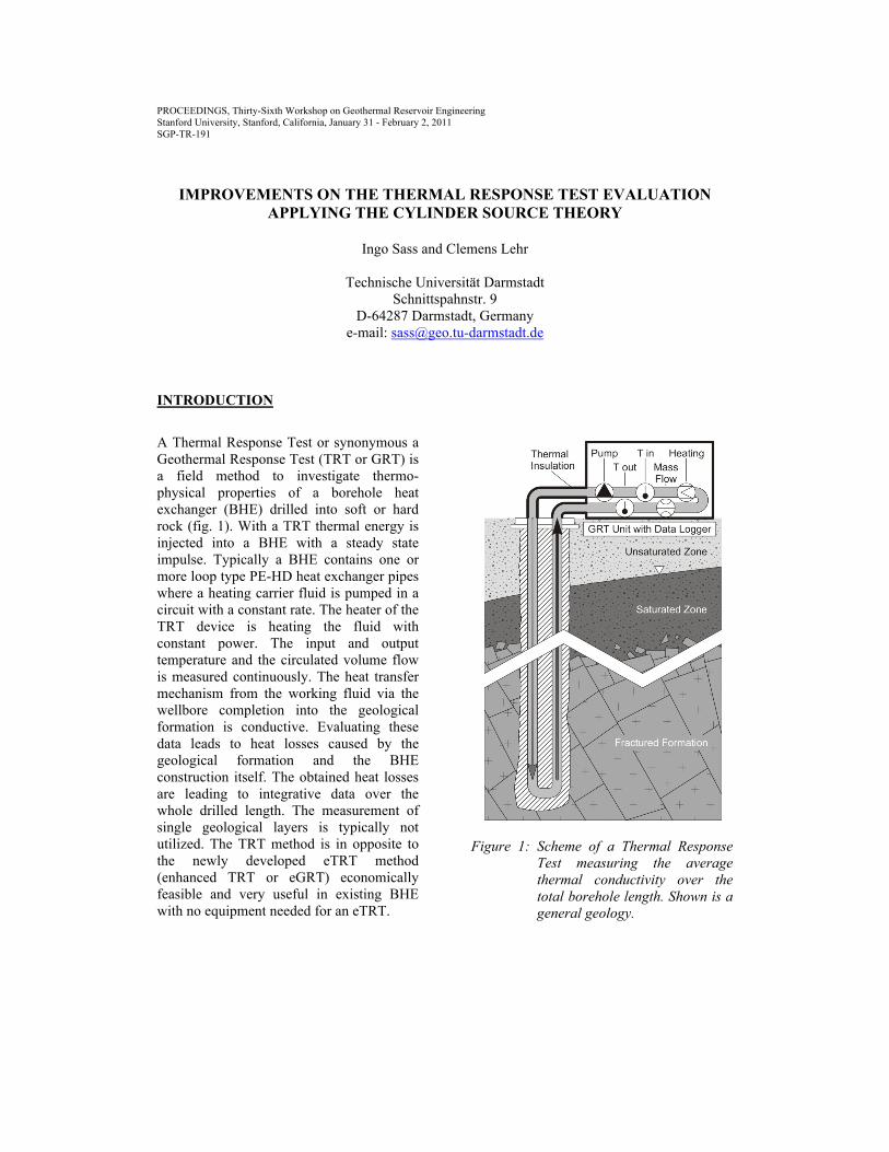
A Thermal Response Test or synonymous a Geothermal Response Test (TRT or GRT) is a field method to investigate thermo-physical properties of a borehole heat exchanger (BHE) drilled into soft or hard rock (fig. 1). With a TRT thermal energy is injected into a BHE with a steady state impulse. Typically a BHE contains one or more loop type PE-HD heat exchanger pipes where a heating carrier fluid is pumped in a circuit with a constant rate. The heater of the TRT device is heating the fluid with constant power. The input and output temperature and the circulated volume flow is measured continuously. The heat transfer mechanism from the working fluid via the wellbore completion into the geological formation is conductive. Evaluating these data leads to heat losses caused by the geological formation and the BHE construction itself. The obtained heat losses are leading to integrative data over the whole drilled length. The measurement of single geological layers is typically not utilized. The TRT method is in opposite to the newly developed eTRT method (enhanced TRT or eGRT) economically feasible and very useful in existing BHE with no equipment needed for an eTRT.

Figure 1: Scheme of a Thermal Response

Test measuring the average thermal conductivity over the total borehole length. Shown is a general geology.

The standard application of a TRT is collecting data for the design and model process of a larger BHE field. Furthermore with a TRT the technical integrity of built BHE can be evaluated. Conventional evaluation (following the line source approach) requires tests durations typically exceeding 50 h to obtain quasi-steady state heat flow conditions. Applying the cylinder source theory enhances the precision of evaluation and reduces the test durations (and therefore cost) because the non-steady state is evaluated. The impact of the GRT-method will increase in the future because real estate business with properties already equipped with borehole heat exchangers need to be valued. The examination of a BHE field in a real estate deal could be a part of a geothermal due diligence. The resulting TRT temperature graph is demonstrating the relation between the injected heat energy and the thermal rock properties. The determination of rock parameters is conventionally done by a line source theory based simplification (Hellström, 1991). Kelvin (1860/61) developed in a theorem of the heat transfer from buried electrical wire lines into the soil his line source concept. Ingersoll & Plass (1948) related Kelvin`s theory to the thermal dynamics for a single U-type borehole heat exchanger and presented a mathematical model. While the mathematical line source model is based on an infinitesimal small line source (Carslaw & Jaeger, 1959). The simplification on the other hand requires a curve fitting regarding the geometry and conditions of a BHE. Those assumptions for the analytical steady state solution of the line source equation with respect to BHE are:

• The resulting subsoil temperature will be replaced by the mean fluid temperature calculated from input and output.

• The undisturbed pre TRT temperature in the geological formation can be obtained from drilling data or is estimated.

• The measuring distance is defined as being equal to the BHE radius.

• The thermal transfer resistance between fluid and borehole wall is introduced

• The effective thermal conductivity is introduced as an average over the total drilled depth as well as the thermal diffusivity.

This line source approach for practical engineering use has some sufficient limitations. Just the overall system thermal conductivity can be obtained from such a TRT evaluation because the substitution of a part of the line source formula the volumetric heat capacity cannot be calculated anymore. Hellström (1991) showed his solution with using a regression equation derived from the input/output temperatures graphs. Therefore the method requires a constant heat input over a sufficient period of time, probably 20 to 100 hours. Else well the data from the starting period of the test have to be excluded from the evaluation due to their non linear unsteady state function (fig. 2).

Figure 2: Typical TRT measurement result.

Shown is the 1st derivation of the data acquisition function a) unsteady state in the initial phase, b) quasi-stationary behavior (straight line phase) and c) the phase where boundary conditions for the heat conduction into the neighbouring formations are changing.

Similar to groundwater pump tests results the early TRT phase behavior shows the level of disturbance of the drilled BHE in detail and requires an evaluation of the unsteady state period. The beginning hours represent influences of the borehole grout, formation damage and convective heat transfer due to water movement driven by the thermal gradients and caused by the reaction heat of the cement based grout. Furthermore the numerical model of BHE fields is becoming more precise if the volumetric heat capacity can be introduced. This paper is showing a quantitative approach to evaluate TRT data with an unsteady state solution following the cylinder source approach (Carslaw & Jaeger, 1956). THEORETICAL BACKGROUND A general solution for the conduction of heat in solids using a source model is introduced by Carslaw & Jaeger (1956). This theory utilizes Green`s function to solve the problems calculating the temperature in any distance from the source of heat. This universal equation [eq. 1] describes the conductive heat transfer from a source with undefined geometry in a homogeneous, isotropic and dry solid:

Based on that equation, solutions for other special source geometries – like point, line or cylinder source – can be derived. A BHE is very long in relation to its small diameter. Ingersoll & Plass (1948) had to follow practical implications to evaluate the performance of the very first BHE. So they had to define some simplifications. This step requires a mono-directional approach: it is not necessary to integrate into x- and y-

direction. This equation is usually written as exponential integral [eq. 2]:

Ingersoll & Plass (1948) were presenting this concept but they could not apply it because there was no explicit solution available. They used an approximate solution [eq. 3]: Recently GRT results are evaluated in using the linear steady state like behaviour (straight line method) which is a simplified derivation from equation 3 [eq. 4]:

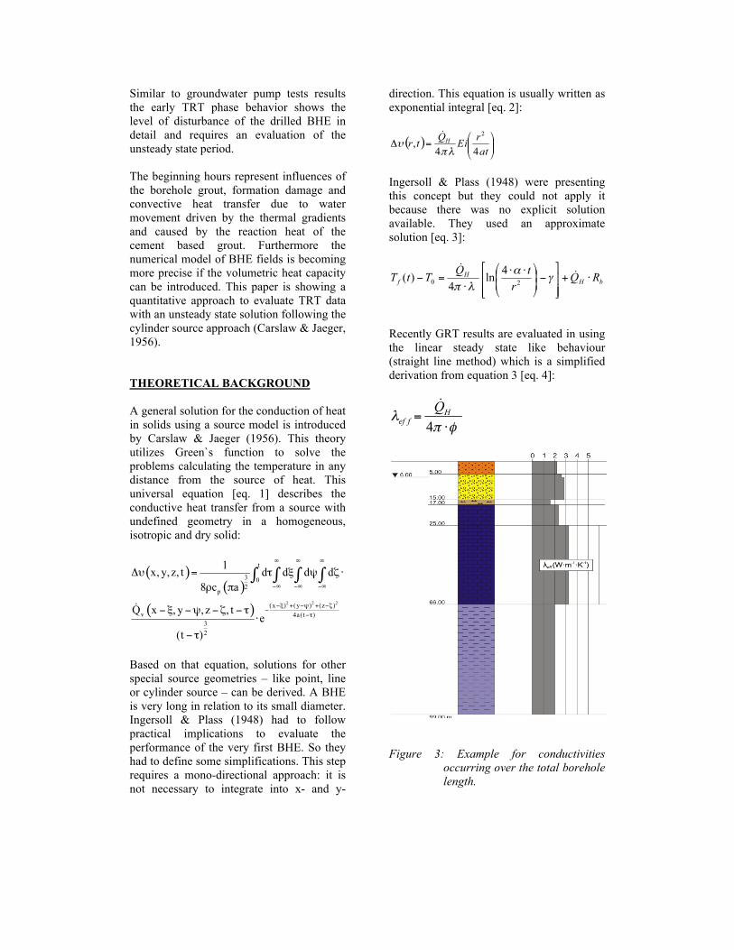
Figure 3: Example for conductivities

occurring over the total borehole length.

Broadly used software solutions like Earth Energy Designer ((most recent EED applies as V3.16) and others. Pre-calculated G-functions (Eskilson, 1984) are used to solve multi but standardized BHE arrays in different geometries with EED to keep the linear analytical solution stable. The apparent result of this evaluation method is the effective thermal conductivity (λeff) which is a time depending integral value over all thermal resistance implemented by a BHE (2.5, fig. 14). The obtained value λeff represents an average of all conductivities occurring over the total borehole length (fig. 3). Systematically this value cannot be used to determine the specific conductivities of single geological layers. As introduced above the volumetric heat capacity then has to be estimated to enter further dimensioning calculations of a BHE array which is not satisfactory for designing purposes. Additionally the thermal transfer resistance of a single BHE can be calculated by the linear approximation [eq. 11] with the straight line data measured by this established method (2.5). Whereas the volumetric heat capacity is only estimated and may vary in a wide range (up to 100% and more), the result for the thermal transfer resistance is fraught with uncertainty. Mogensen (1983) has demonstrated that a mistake of 20% for the estimated heat capacity leads to an error of 10% for the thermal transfer resistance. It may be remarked here, that the value for the thermal transfer resistance got from a TRT is only valid at test conditions. There are dynamic partial resistances (mass flow depending on the heat exchanger fluid and groundwater) which are affecting the thermal transfer resistance in nearly all TRT phases over all [eq. 5]:

To use both methods it is necessary to operate a TRT into a quasi steady state. This

requires long measuring times defined by a minimum time criterion after Eskilson (1987) [eq.6, simplified]:

20 to 100 h test time is reasonable for the most occasions. The practical problem with this criterion is that the high energy consuming TRT with 3 to 12 KW power is becoming very cost intensive and slight changes in the power supply lead to invalid results because the straight line condition will be violated. Also hydrogeological conditions may change (rising/falling piezometric head) within the test period. Another dominant error source is the application of low test powers. The result is that the steady state condition will not be maintained long enough to provide a small experimental error. GENERAL The line source theory is only valid, if the boundary conditions for the top and bottom of the line source are specified adiabatic. Natural conditions of a BHE are far from that. Extreme conditions, like a BHE which is installed under a whole year snow covered area and drilled into a granite which is underlain by an almost impermeable clay would meet the requirements of the line source theory. However the disturbing axial thermal flux which shall not take place in accordance to the line source theory cannot be stopped technically. As a matter of fact it is necessary to consider axial thermal flux evaluating TRT data. The impact of the axial flux depends primarily on the height/width ratio of the BHE itself. Additionally, the boundary conditions given by the geological and hydrogeological conditions surrounding the BHE may influence the axial flux significantly.

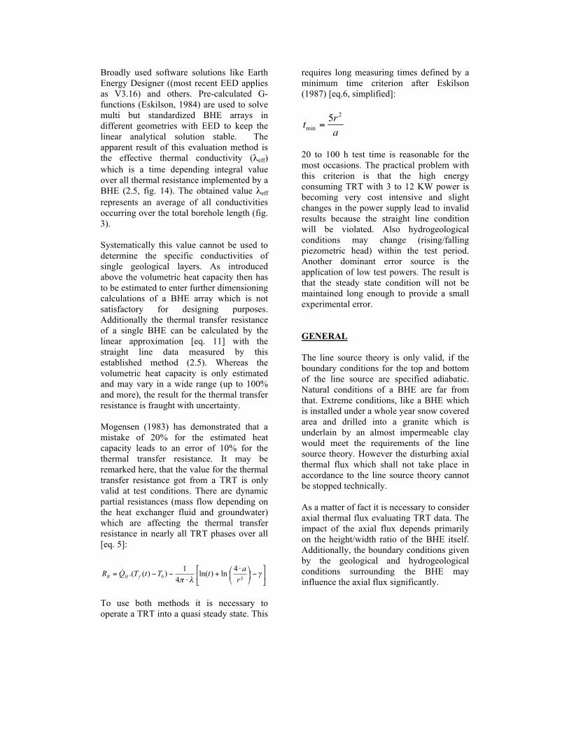
Figure 4: Comparison of line source and

cylinder source approach with constant thermal conductivity, volumetric heat capacity and power input varying the height/width ratio of the BHE (calculated with Numericallnt, Geologik Software).

The cylinder source approach enables to introduce both – radial and axial thermal flux. Figure 4 shows the comparison of line source and cylinder source in a normalized graph. Figure 4 shows that the time-dependence of the curves varies in a wide range if the height/width ratio will be changed. The line source approach is not congruent to the cylinder source approach at all. Only for a width/height ratio greater than 1: 1000 and long runtimes the shape of the line source approach follows close to the cylinder source graph. On one hand it can be demonstrated that the values which are evaluated with a line source approach are afflicted by growing errors with increasing axial flux. On the other the cylinder approach is valid over the whole runtime obviously. Resuming the above mentioned facts the cylinder source

method is a great improvement to evaluate and reproduce (2.3) TRT in any geological and technical (BHE, energy piles, energy baskets, complex grids, etc.) environment. CYLINDER SOURCE APPROACH The line source approach is not matching real test data close to the origin of the curve (unsteady heat flow conditions in the start-up phase of a TRT) This is because the axial thermal flow cannot be denied. If equation 1 is transferred to cylinder coordinates the equation [eq. 7] becomes:

Using the cylinder functions after Bessel the cylinder source term can be simplified as shown with equation 8 and is useable for evaluating TRT data:

For evaluating TRT data the mean fluid temperature between Tin and Tout has to be determined. Since a BHE has a radial symmetry, the logarithmic mean temperature at the half length of the completed depth has to be calculated. The arithmetic mean temperature is only valid for heat transfer at planar elements. The logarithmic mean temperature describes the in-situ conditions in tube bundle heat exchangers (u-tube BHE) very well if radial heat transfer can be considered (Rogers & Mayhew 1967). The logarithmic mean temperature of a TRT can be calculated as follows [eq. 9]:

With the logarithmic mean temperature the effective thermal conductivity and effective volumetric heat capacity can be determined by inverse modelling. The problem can be solved with cylinder source approach. Fitted values for λeff, ρc, Peff and RBeff with known QH have to be applied to match the calculated curve on the measured curve. Fast and precise results are obtained when the fit is computed by algorithms like Nelder-Mead-Method (Nelder & Mead 1965) or similar algorithms. However both, line and cylinder source evaluation as described before, require constant heat power input. Fluctuating heat power input leads to unsteady behaviour of the measured temperature curve throughout the test. Such conditions are often reality at construction sites. Non stable voltage in the test phase is given because many devices are connected to one main power supply. Such influenced measurements can be evaluated by time depending superposition. The principle of superposition leads to equation 10 for the line source approach

which gives equation 11 for the cylinder source approach:

TEST SITE DATA EVALUATION

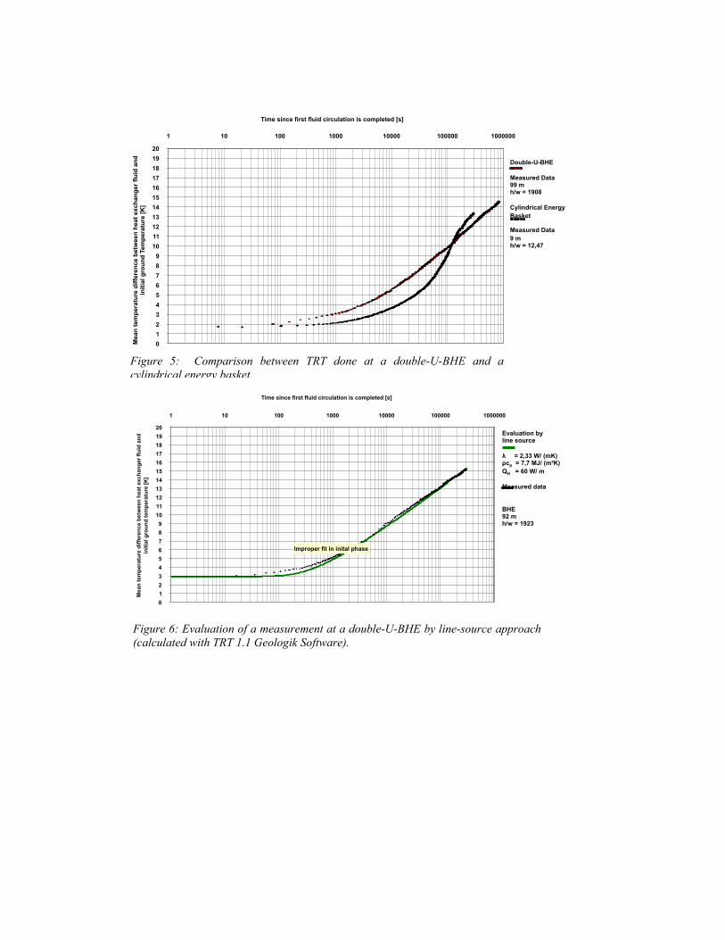
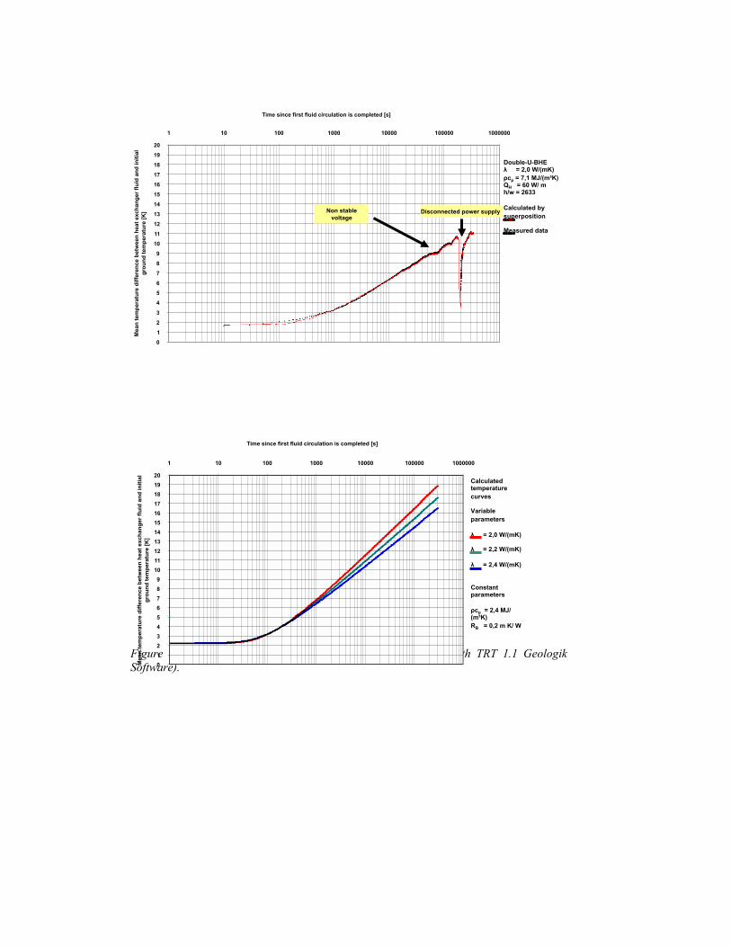
The following figures show measurement data from real BHE tests. Figure 5 shows measurements at a double-U-BHE and a cylindrical energy basket. The measurements at test sites show that the theoretical characteristics as shown in figure 4 match well to these data. Figure 6 and 7 show the difference between the evaluation of a measurement at a double-U-BHE using line source and cylinder source approach. The cylinder source approach fits to the measured data while the line source approach has an improper fit especially in the initial phase of the TRT. Due to the different heat transfer geometries of the line source and the cylinder source approach contradictious achievements will be obtained. As figure 8 shows is the difference of the results between these evaluation methods getting much more significant if the width/height ratio of the heat exchanger gets smaller. The cylinder source approach fits well over the whole runtime while the line source approach is only fitting in a late “quasi-straight-line-phase”. The error by evaluating data from measurements done at heat exchangers with such geometries - like energy baskets or energy piles - by line source approach can be larger than 100%. Figure 9 shows a measurement under problematical test site conditions. Non stable voltage and temporary disconnection of the power supply by workers at the test site led to a discontinuously power input and run of the measured temperature curve. Such data can be evaluated by the principle of time dependent superposition.

0 1 2 3 4 5 6 7 8 9

10 11 12 13 14 15 16 17 18 19 20

1 10 100 1000 10000 100000 1000000 M

ean

tem

pera

ture

diff

eren

ce b

etw

een

heat

exc

hang

er fl

uid

and

initi

al g

roun

d Te

mpe

ratu

re [K

]

Time since first fluid circulation is completed [s]

Double-U-BHE

Measured Data 99 m h/w = 1908

Cylindrical Energy Basket

Measured Data 9 m h/w = 12,47

0 1 2 3 4 5 6 7 8 9

10 11 12 13 14 15 16 17 18 19 20

1 10 100 1000 10000 100000 1000000

Mea

n te

mpe

ratu

re d

iffer

ence

bet

wee

n he

at e

xcha

nger

flui

d an

d in

itial

gro

und

tem

pera

ture

[K]

Time since first fluid circulation is completed [s]

Evaluation by line source

λ = 2,33 W/ (mK) ρcp = 7,7 MJ/ (m³K) QH = 60 W/ m

Measured data

BHE 92 m h/w = 1923

Improper fit in inital phase

Figure 5: Comparison between TRT done at a double-U-BHE and a cylindrical energy basket.

Figure 6: Evaluation of a measurement at a double-U-BHE by line-source approach (calculated with TRT 1.1 Geologik Software).

)

0 1 2 3 4 5 6 7 8 9

10 11 12 13 14 15 16 17 18 19 20

1 10 100 1000 10000 100000 1000000

Mea

n te

mpe

ratu

re d

iffer

ence

bet

wee

n he

at e

xcha

nger

flui

d an

d in

itial

gro

und

tem

pera

ture

[K]

Time since first fluid circulation is completed [s]

Evaluation by line source

λ = 5,5 W/(mK) ρcp = 1,8 MJ/(m³K) QH = 560 W/m

Evaluation by cylinder source

λ = 2,4 W/(mK) ρcp = 3,6 MJ/(m³K) QH = 560 W/m

Measured data

Energy basket h = 9 m

0 1 2 3 4 5 6 7 8 9

10 11 12 13 14 15 16 17 18 19 20

1 10 100 1000 10000 100000 1000000 M

ean

tem

pera

ture

diff

eren

ce b

etw

een

heat

exc

hang

er fl

uid

and

initi

al g

roun

d te

mpe

ratu

re [K

]

Time since first fluid circulation is completed [s]

Evaluation by cylinder source

λ = 2,2 W/(mK) ρcp = 8,9 MJ/(m³K) QH = 60 W/ m

Measured data

BHE 92 m h/w = 1923

Figure 7: Evaluation of a measurement at a double-u-BHE by cylinder source approach (calculated with TRT 1.1 Geologik Software).

Figure 8: Evaluation of a measurement at a cylindrical energy basket by line and cylinder source approach (calculated with TRT 1.1 Geologik Software).

0

1

2

3

4

5

6

7

8

9

10

11

12

13

14

15

16

17

18

19

20

1 10 100 1000 10000 100000 1000000 M

ean

tem

pera

ture

diff

eren

ce b

etw

een

heat

exc

hang

er fl

uid

and

initi

al

grou

nd te

mpe

ratu

re [K

]

Time since first fluid circulation is completed [s]

Double-U-BHE λ = 2,0 W/(mK) ρcp = 7,1 MJ/(m³K) QH = 60 W/ m h/w = 2633

Calculated by superposition

Measured data

Non stable voltage

Disconnected power supply

Figure 9: Evaluation by time based superposition (calculated with TRT 1.1 Geologik Software).

0 1 2 3 4 5 6 7 8 9

10 11 12 13 14 15 16 17 18 19 20

1 10 100 1000 10000 100000 1000000

Mea

n te

mpe

ratu

re d

iffer

ence

bet

wee

n he

at e

xcha

nger

flui

d an

d in

itial

gr

ound

tem

pera

ture

[K]

Time since first fluid circulation is completed [s]

Calculated temperature curves

Variable parameters

λ = 2,0 W/(mK)

λ = 2,2 W/(mK)

λ = 2,4 W/(mK)

Constant parameters

ρcp = 2,4 MJ/(m³K) RB = 0,2 m K/ W QH = 60 W/m

0 1 2 3 4 5 6 7 8 9

10 11 12 13 14 15 16 17 18 19 20

1 10 100 1000 10000 100000 1000000

Mea

n te

mpe

ratu

re d

iffer

ence

bet

wee

n he

at e

xcha

nger

flui

d an

d in

itial

gro

und

tem

pera

ture

[K]

Time since first fluid circulation is completed [s]

Calculated temperature curves

Variable parameters

ρcp = 1,0 MJ/(m³K)

ρcp = 2,0 MJ/(m³K)

ρcp = 3,0 MJ/(m³K)

ρcp = 4,0 MJ/(m³K)

Constant parameters

QH = 60 W/m RB = 0,2 m K/W λ = 2,4 W/mK

BHE

Figure 11: Sensitivity analysis for volumetric heat capacity (calculated with TRT 1.1 Geologik Software).

0

1

2

3

4

5

6

7

8

9

10

11

12

13

14

15

16

17

18

19

20

1 10 100 1000 10000 100000 1000000

Mea

n te

mpe

ratu

re d

iffer

ence

bet

wee

n he

at e

xcha

nger

flui

d an

d in

itial

gro

und

tem

pera

ture

[K]

Time since first fluid circulation is completed [s]

Calculated temperature curves

Variable parameters

QH = 50 W/m

QH = 60 W/m

QH = 70 W/m

Constant parameters

ρcp = 2,4 MJ/(m³K) RB = 0,1 m K/W λ = 2,4 W/mK

BHE 92 m h/w = 1923

Figure 12: Sensitivity analysis for heating power (calculated with TRT 1.1 Geologik Software).

SENSITIVITY AND ERRORS

The following figures show a sensitivity analysis on the parameters which affecting the plot of the temperature curves got from a GRT. As figures 10 to 13 show, affect all four parameters the run of the curve significantly. Only the correct combinations of these parameters lead to a proper fit and evaluation. If the undisturbed temperature of the ground at the start of the measurement (Signorelli 2004), the heating power and the thermal resistivity (eq. 12) are determined properly, there are no multiple solutions given. It has to be considered that the values for the thermal conductivity, the volumetric heat capacity and the thermal resistivity obtained from a TRT are averaged and affected by multi-compartments over the whole borehole length. That is why values got from a TRT should not be used in numerical

calculations which separate in conductive and convective heat transport algorithms.

THERMAL BOREHOLE RESISTIVITY

There are several part-resistances which are affecting the value of the total thermal resistance of a BHE (fig. 14). Resistivity of the material: heat exchanger fluid (R3), polyethylene pipes (R4), borehole grout material (R2). Resistivity by contact: borehole wall (skin zone) – grout (R1), pipes-grout (R4), drilling skin zone (Rs). Dynamic resistance: mass flow of the heat exchanger fluid (laminar, turbulent) and groundwater flow. There are different possibilities to determine the thermal resistivity of a BHE. As mentioned before, the value for the thermal transfer resistance got from a TRT is valid only for the specific test conditions. There are dynamic partial resistances (mass flow depending on the heat exchanger fluid and groundwater) which are affecting the

0

1

2

3

4

5

6

7

8

9

10

11

12

13

14

15

16

17

18

19

20

1 10 100 1000 10000 100000 1000000

Mea

n te

mpe

ratu

re d

iffer

ence

bet

wee

n he

at e

xcha

nger

flui

d an

d

initi

al g

roun

d te

mpe

ratu

re [K

]

Time since first fluid circulation is completed [s]

Calculated temperature curves

Variable parameters

RB = 0,1 mK/W

RB = 0,2 mK/W

RB = 0,3 mK/W

Constant parameters

QH = 60 W/m ρcp = 2,4 MJ/(m³K) λ = 2,4 W/mK

BHE 92 m

Figure 13: Sensitivity analysis for thermal resistance (calculated with TRT 1.1 Geologik Software).

thermal transfer resistance in every all TRT phases over all.

Figure 14: Schematic cross section through

a BHE showing all thermal resistances influencing the horizontal heat transfer (without dynamic resistances).

Equation 12 shows a possibility to determine the value for RBeff using the logarithmic mean temperature in relation to the specific heat input. Performing a GRT all needed input parameters for the calculation will be measured. Energy that is not transmitted to the ground is in relation to the thermal resistance:

The beginning of a TRT shows the thermal resistance occurring by a BHE (fig. 15). The starting phase as shown in figure 15 is typical and occurs in that way in every TRT. The data plot demonstrates each single part-resistance (RB) of the system. The first interaction (fig. 15) between hot and cold rail takes place before the first heat exchanger fluid circulation is completed. This is because the temperature gradient of the heated heat exchanger fluid is affecting the cold rail while the first turnaround is still ongoing. When the first circulation is

completed the resistivity of the BHE including the intern losses can be calculated.

Figure 15: Resistance by a BHE 1)

Resistivity of the pipe (blue), 2) Dynamic resistance including heat losses between hot and cold rail (red), 3) Bulk-resistance including the mass and resistance of the borehole grout (green).

This is the starting point of a TRT. Here the inclination of the upgrading temperature curve is increasing. Within the subsequent test the curve is slightly flattening. The reason for this typical thermal behaviour is that the induced heat flow has to overcome the resistance of the grout and skin zone. The transport of heat into the undisturbed geological formation which follows can be withdrawn from the further temperature development. CONCLUSIONS The comparison between mathematical theory and test site data shows that the cylinder source approach is the more precise evaluation method for Thermal Response Tests in any geological environment. On one hand it can be demonstrated, that the values, which are calculated with a line source approach, are afflicted by growing errors with increasing axial flux. On the other the cylinder approach is valid over the whole runtime obviously. The straight line approach is only acceptable in stationary and radial symmetrical conditions if very simple geological

conditions are considered. A tolerable error level can only be obtained if a heat exchanger length to width ration larger than 1000:1 is postulated. The simplifying derivations which are used in common practice of applying the straight line approach is leading to a complete loss of all information about the BHE and boundary conditions. The cylinder source approach derived and applied in this study allows to evaluate TRT data in the non-steady state and in the quasi-stationary state. It is new that measurements with changing power input can be evaluated by time based superposition. Such data is invalid for the simplified linear line source approach. This may lead to shorter times of measurement in future applications. Furthermore the effective volumetric heat capacity can be determined. The value of this parameter may be much higher than the value obtained from measurements under (pseudo)-static conditions in laboratory (i.e. values shown in VDI, 2001). The groundwater flow is affecting this parameter as well as the thermal conductivity. Due to the physical properties of water (low thermal conductivity, high volumetric heat capacity) the value for the shallow geothermal system`s heat capacity will be affected markedly by groundwater flow. LITERATURE Lord Kelvin 1860/61. On the reduction of observations of underground temperature. Transactions of the Royal Society of Edinburgh Vol. 22. Rogers, G., Mayhew, Y. 1967. Engineering Thermodynamics Work and Heat Transfer, Fourth Edition. Pearson Education Limited, Great Britain. Ingersoll, L.R., Plass H.J. 1948. Theory of Ground Pipe Heat Source for the Heat Pump. ASHVE Transactions 47, 339-348, Chicago.

Hellström, G. 1991. Ground Heat Storage, Thermal Analysis of Duct Storage Systems, I. Theory. 282 p., Dept. Mathematical Physics, University of Lund, Sweden. Mogensen, P. 1983. Fluid to Duct Wall Heat Transfer in Duct System Heat Storages. Proceedings of the International Conference on Subsurface Heat Storage in Theory and Practice. Swedish Council for Building Research. Stockholm, Sweden, June 6-8, 1983, p. 652-657. Nelder, J.A., Mead, R. 1965. A simple Method for Function Minimization. Computer Journal 7(1), 308-313. Sanner, B. et al. 2007. Technology, development status, and routine application of Thermal Response Test. Proceedings European Geothermal Congress 2007. Unterhaching, Germany, 30 May-1 June. Carslaw, H.S., Jaeger, J.C. 1959. Conduction of Heat in Solids, Second Edition, Oxford University Press, Great Britain. Eskilson, P. 1984. Thermal Analysis of Heat Extraction Boreholes. Lund-MPh-87/13. Dept. Of Mathematical Physics, Lund Institute of Technology, Sweden. Gehlin, S. 2002. Thermal response test – Method development and evaluation. Doctoral Thesis 2002:39. Lund Institute of Technology, Sweden. Signorelli, S. 2004. Geoscientific Investigations for the use of Shallow Low-Enthalpy Systems. Doctoral Thesis 2004. Swiss Federal Institute of Technology Zurich, Switzerland. VDI (ed.) 2001. VDI-Guideline 4640: Thermal use of the underground – Ground source heat pump systems. Beuth, Berlin.

LIST OF SYMBOLS

 a Thermal Diffusivity [m2/s] 8cp Volumetric Heat Capacity [MJ/(m³ K)] Erf Gaussian Error Function H Length of BHE [m] Ei Exponential Integral IO(x) Cylinder Function after Bessel l Length of Pipe [m]

Specific Heat Input [W/m] r Effective Radius of the Heat Source [m] r1 Inner Radius of Pipe [m] r2 Outer Radius of Pipe [m] R Radius of Cylinder Source [m] RB Thermal Resistivity [K m/W] RBeff Effective Thermal Resistivity [K m/W] Tf Mean Temperature of the Heat

Exchanger Fluid [°C]

T0   Average undisturbed Temperature of Ground [°C]

t Time [s] x,y,z Cartesian Coordinates Function of Time in Input Temperature of Heat Exchanger Fluid [°C] out Output Temperature of Heat

Exchanger Fluid [°C]

0 Average undisturbed Temperature of Ground [°C]

Difference of Temperature [K]

1 Inner Temperature of Pipe on r1 [°C] 2 Outer Temperature of Pipe on r2 [°C] 6 Pi 3.141…. Temperature [°C] Time dependent Function over Radius ,,5 Time dependent Functions over

x,y,z Direction        

Euler Constant 0.5772.. 2 Thermal Conductivity [W/(mK)] 2Eff Effective Thermal Conductivity [W/(mK)] 2Material Thermal Conductivity of a Material

(i.e. grout, polyethylene) [W/(mK)]

Inclination of Temperature Curve over Logarithmical Time Scale