Improved Sub-pixel Stereo Correspondencesthrough...
7
Improved Sub-pixel Stereo Correspondences through Symmetric Refinement Diego Nehab 1 Szymon Rusinkiewicz 1 James Davis 2 1 Princeton University 2 University of California at Santa Cruz Abstract Most dense stereo correspondence algorithms start by es- tablishing discrete pixel matches and later refine these matches to sub-pixel precision. Traditional sub-pixel refine- ment methods attempt to determine the precise location of points, in the secondary image, that correspond to discrete positions in the reference image. We show that this strategy can lead to a systematic bias associated with the violation of the general symmetry of matching cost functions. This bias produces random or coherent noise in the final reconstruc- tion, but can be avoided by refining both image coordinates simultaneously, in a symmetric way. We demonstrate that the symmetric sub-pixel refinement strategy results in more accurate correspondences by avoiding bias while preserv- ing detail. 1. Introduction The computation of precise sub-pixel stereo correspon- dences is vital to areas such as 3D scanning and image based modeling and rendering. Most dense stereo correspondence algorithms start by determining discrete pixel matches and later refine these matches to sub-pixel precision [11]. The initial set of correspondences is usually computed by mini- mization of a matching cost function that has been laid out as a disparity space image (DSI) [2, 14]. Sub-pixel refinement of correspondences can be per- formed over a finely sampled or continuously reconstructed neighborhood of the DSI around the initial integer match. The continuous reconstruction strategy has the advantage of being simple and efficient. On the other hand, although computationally more expensive, the supersampling alter- native tends to be more accurate. Efforts have been made both to improve the quality of reconstruction-based refine- ment [12, 13] and to improve the efficiency of supersam- pling [6]. In this paper, we identify a new source of bias for reconstruction-based sub-pixel refinement strategies (sec- tion 2). It can be observed when one image is considered as reference and the refinement is performed on the corre- sponding coordinate in the matching image. It arises from the sensitivity of this “traditional” approach to the varying confidence of the matching cost function when evaluated at neighboring pixels. In the final reconstruction, the bias can (a) (b) (c) (d) Figure 1: Examples of matching cost functions. (a) Sum of squared differences. (b) Normalized cross-correlation. (c) Birchfield and Tomasi [1]. (d) Sum of absolute differences. Note the matching ridge and how the functions are symmetric with regard to it. be experienced as random or coherent noise, as the “texture embossing” addressed by Curless and Levoy [4], or as the “striping effect” addressed by Zhang et al. [16]. To avoid bias, our symmetric sub-pixel refinement strat- egy refines both the reference and the matching image co- ordinates simultaneously, in a symmetric way, by looking for the minimum of the matching cost function along a di- rection that is insensitive to its confidence variations (sec- tion 3). We present results on both synthetic data and real scans obtained using active stereo (section 4), which show that this new method significantly reduces bias in high- variance situations. Additionally, we demonstrate that one of its variants avoids the “pixel locking” effect addressed by Shimizu and Okutomi [12]. 2. The Symmetry of Matching Cost Consider two rectified cameras C 1 and C 2 , producing im- ages I 1 and I 2 of an object, such that the scan-lines in each image are corresponding epipolar lines [7]. In this setup, Yang et al. [14] reduced the problem of stereo matching to that of finding a surface in the disparity-space image Ξ(x 1 ,y,d), which measures the cost of matching points (x 1 ,y) in I 1 and (x 1 + d, y) in I 2 . The matching cost is de- fined by a metric M that compares neighborhoods of pixel values, so that Ξ(x 1 ,y,d) ≡ M (I 1 (x 1 ,y),I 2 (x 1 + d, y)). Note that for a given scan-line y, the problem simplifies even further to that of finding a matching ridge, which is the extremum curve in Ξ y (x 1 ,d). Instead of working in disparity space, we prefer to work directly with image coordinates. The concept of disparity implies taking one camera as reference and, as we shall see, this is a source of bias. The direct parameterization F y (x 1 ,x 2 ) ≡ Ξ y (x 1 ,x 2 - x 1 ) is more symmetric and sim- plifies our analysis. Figure 1 shows examples of popular 1
Transcript of Improved Sub-pixel Stereo Correspondencesthrough...

Improved Sub-pixel Stereo Correspondences through Symmetric Refinement
Diego Nehab1 Szymon Rusinkiewicz1 James Davis2
1Princeton University 2University of California at Santa Cruz
Abstract
Most dense stereo correspondence algorithms start by es-
tablishing discrete pixel matches and later refine these
matches to sub-pixel precision. Traditional sub-pixel refine-
ment methods attempt to determine the precise location of
points, in the secondary image, that correspond to discrete
positions in the reference image. We show that this strategy
can lead to a systematic bias associated with the violation of
the general symmetry of matching cost functions. This bias
produces random or coherent noise in the final reconstruc-
tion, but can be avoided by refining both image coordinates
simultaneously, in a symmetric way. We demonstrate that
the symmetric sub-pixel refinement strategy results in more
accurate correspondences by avoiding bias while preserv-
ing detail.
1. Introduction
The computation of precise sub-pixel stereo correspon-
dences is vital to areas such as 3D scanning and image based
modeling and rendering. Most dense stereo correspondence
algorithms start by determining discrete pixel matches and
later refine these matches to sub-pixel precision [11]. The
initial set of correspondences is usually computed by mini-
mization of a matching cost function that has been laid out
as a disparity space image (DSI) [2, 14].
Sub-pixel refinement of correspondences can be per-
formed over a finely sampled or continuously reconstructed
neighborhood of the DSI around the initial integer match.
The continuous reconstruction strategy has the advantage
of being simple and efficient. On the other hand, although
computationally more expensive, the supersampling alter-
native tends to be more accurate. Efforts have been made
both to improve the quality of reconstruction-based refine-
ment [12, 13] and to improve the efficiency of supersam-
pling [6].
In this paper, we identify a new source of bias for
reconstruction-based sub-pixel refinement strategies (sec-
tion 2). It can be observed when one image is considered
as reference and the refinement is performed on the corre-
sponding coordinate in the matching image. It arises from
the sensitivity of this “traditional” approach to the varying
confidence of the matching cost function when evaluated at
neighboring pixels. In the final reconstruction, the bias can
(a) (b) (c) (d)
Figure 1: Examples of matching cost functions. (a) Sum of squareddifferences. (b) Normalized cross-correlation. (c) Birchfield andTomasi [1]. (d) Sum of absolute differences. Note the matchingridge and how the functions are symmetric with regard to it.
be experienced as random or coherent noise, as the “texture
embossing” addressed by Curless and Levoy [4], or as the
“striping effect” addressed by Zhang et al. [16].
To avoid bias, our symmetric sub-pixel refinement strat-
egy refines both the reference and the matching image co-
ordinates simultaneously, in a symmetric way, by looking
for the minimum of the matching cost function along a di-
rection that is insensitive to its confidence variations (sec-
tion 3). We present results on both synthetic data and real
scans obtained using active stereo (section 4), which show
that this new method significantly reduces bias in high-
variance situations. Additionally, we demonstrate that one
of its variants avoids the “pixel locking” effect addressed
by Shimizu and Okutomi [12].
2. The Symmetry of Matching Cost
Consider two rectified cameras C1 and C2, producing im-
ages I1 and I2 of an object, such that the scan-lines in each
image are corresponding epipolar lines [7]. In this setup,
Yang et al. [14] reduced the problem of stereo matching
to that of finding a surface in the disparity-space image
Ξ(x1, y, d), which measures the cost of matching points
(x1, y) in I1 and (x1 + d, y) in I2. The matching cost is de-
fined by a metric M that compares neighborhoods of pixel
values, so that Ξ(x1, y, d) ≡ M(I1(x1, y), I2(x1 + d, y)).Note that for a given scan-line y, the problem simplifies
even further to that of finding a matching ridge, which is
the extremum curve in Ξy(x1, d).Instead of working in disparity space, we prefer to work
directly with image coordinates. The concept of disparity
implies taking one camera as reference and, as we shall
see, this is a source of bias. The direct parameterization
Fy(x1, x2) ≡ Ξy(x1, x2 − x1) is more symmetric and sim-
plifies our analysis. Figure 1 shows examples of popular
1
q2
C1 C2
p2
P
p1
ZZQ
X2X1
r2(t)r1(t)
U
u q1
Oy(t)
Figure 2: The slope of the matching ridge. The geometry of thesetup yields an expression for the slope dr2/dr1, as given by equa-tion 6. Each intersection U between the object tangent and thebaseline of the cameras produces a different slope.
matching cost functions under this direct parametrization.
In each case, the matching ridge is clearly visible. We also
notice a certain symmetry of the matching cost, which we
explain below.
Consider the intersection between the object being im-
aged and a given epipolar plane, as shown in figure 2. It
defines a curve Oy(t) that is projected into I1 and I2. If
r1(t) and r2(t) are the corresponding parametrizations for
these projections, the matching ridge is simply the curve de-
fined by Ry(t) = (r1(t), r2(t)). Given a perfect matching
pair (x1, x2), it is clear that Ry goes through (x1, x2) for
some t. If r1 and r2 are continuous and smooth at t, then
(x1 + dr1(t), x2 + dr2(t)) is a first order approximation
for Ry . It follows that (x1 ± dr1, x2 ± dr2) are also on the
matching ridge and therefore are also matching pairs.
Comparing the values of Fy(x1 + dr1, x2 − dr2) and
Fy(x1−dr1, x2+dr2), we notice that they must be similar:
Fy(x1 + dr1, x2 − dr2) ≡
≡ M(I1(x1 + dr1, y), I2(x2 − dr2, y)) (1)
= M(I2(x2 − dr2, y), I1(x1 + dr1, y)) (2)
≈ M(I1(x1 − dr1, y), I1(x1 + dr1, y)) (3)
≈ M(I1(x1 − dr1, y), I2(x2 + dr2, y)) (4)
≡ Fy(x1 − dr1, x2 + dr2) (5)
Steps (1) and (5) are by definition. Step (2) follows from
the symmetry of M . Steps (3) and (4) come first from the
fact that, since x1 ± dr1 matches x2 ± dr2, I1(x1 ± dr1, y)must be similar to I2(x2 ± dr2, y). The continuity of M
then leads to the approximations.
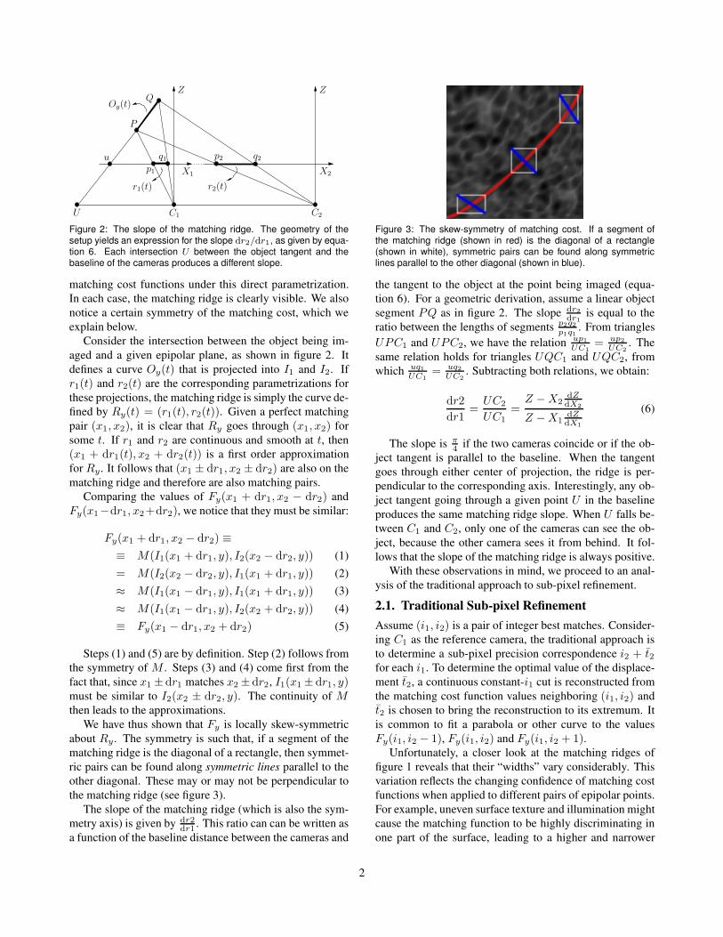
We have thus shown that Fy is locally skew-symmetric
about Ry . The symmetry is such that, if a segment of the
matching ridge is the diagonal of a rectangle, then symmet-
ric pairs can be found along symmetric lines parallel to the
other diagonal. These may or may not be perpendicular to
the matching ridge (see figure 3).
The slope of the matching ridge (which is also the sym-
metry axis) is given by dr2
dr1. This ratio can can be written as
a function of the baseline distance between the cameras and
Figure 3: The skew-symmetry of matching cost. If a segment ofthe matching ridge (shown in red) is the diagonal of a rectangle(shown in white), symmetric pairs can be found along symmetriclines parallel to the other diagonal (shown in blue).
the tangent to the object at the point being imaged (equa-
tion 6). For a geometric derivation, assume a linear object
segment PQ as in figure 2. The slope dr2
dr1
is equal to the
ratio between the lengths of segments p2q2
p1q1
. From triangles
UPC1 and UPC2, we have the relation up1
UC1
= up2
UC2
. The
same relation holds for triangles UQC1 and UQC2, from
which uq1
UC1
= uq2
UC2
. Subtracting both relations, we obtain:
dr2
dr1=
UC2
UC1
=Z − X2
dZdX2
Z − X1dZdX1
(6)
The slope is π4
if the two cameras coincide or if the ob-
ject tangent is parallel to the baseline. When the tangent
goes through either center of projection, the ridge is per-
pendicular to the corresponding axis. Interestingly, any ob-
ject tangent going through a given point U in the baseline
produces the same matching ridge slope. When U falls be-
tween C1 and C2, only one of the cameras can see the ob-
ject, because the other camera sees it from behind. It fol-
lows that the slope of the matching ridge is always positive.
With these observations in mind, we proceed to an anal-
ysis of the traditional approach to sub-pixel refinement.
2.1. Traditional Sub-pixel Refinement
Assume (i1, i2) is a pair of integer best matches. Consider-
ing C1 as the reference camera, the traditional approach is
to determine a sub-pixel precision correspondence i2 + t̄2for each i1. To determine the optimal value of the displace-
ment t̄2, a continuous constant-i1 cut is reconstructed from
the matching cost function values neighboring (i1, i2) and
t̄2 is chosen to bring the reconstruction to its extremum. It
is common to fit a parabola or other curve to the values
Fy(i1, i2 − 1), Fy(i1, i2) and Fy(i1, i2 + 1).Unfortunately, a closer look at the matching ridges of
figure 1 reveals that their “widths” vary considerably. This
variation reflects the changing confidence of matching cost
functions when applied to different pairs of epipolar points.
For example, uneven surface texture and illumination might
cause the matching function to be highly discriminating in
one part of the surface, leading to a higher and narrower
2

(a) (b)
(c) (d)
Figure 4: Uncertainty bumps. (a) Sliding an axis-aligned cut acrossuncertainty bumps causes bias. (c) On the other hand, cuts alignedto the symmetric lines of the matching cost function are insensitiveto the bumps. Figures (b, d) show schematic views of the real datashown in figures (a, c). Curved lines show a hypothetical uncertaintybump and dashed lines show the cut directions.
ridge. Elsewhere, the matches might be more ambiguous,
leading to a lower and flatter ridge.
As we compute the sub-pixel matches for each i1, we
slide the constant-i1 cut past several of these uncertainty
bumps in the matching ridge. As each bump goes by, the
fit is biased first to one side, then to the other. Figure 4(a)
shows the phenomenon in real data, and figure 4(b) explains
why it happens schematically. This bias is responsible for
most of the noise seen in the “traditional” reconstructions
of figures 7 and 8.
As suggested by figures 4(c) and 4(d), we can avoid this
problem if we look for the extrema along the symmetric
lines of the matching cost function. Neither camera is con-
sidered as reference, and the refined matches will have sub-
pixel precision in the coordinates of both images. This is
the fundamental idea behind our symmetric sub-pixel re-
finement method.
3. Symmetric Sub-pixel Refinement
Guided by the desire to capture the symmetry of the match-
ing cost function, we consider a 2D neighborhood of match-
ing cost values around (i1, i2), and reconstruct a contin-
uous surface S(t1, t2) from it. We then define C(t) =S(s1t, s2t), a cut through the reconstruction in the [s1 s2]
T
direction. The symmetric sub-pixel refined match is given
by the pair (i1 + s1t̄, i2 + s2t̄), where [s1 s2]T follows the
lines of symmetry of matching cost, and t̄ is chosen to bring
the cut to its extremum.
All that is left to do is choose the surface reconstruction
method and find the direction of the cut. Below we investi-
gate some options.
3.1. Quadric Interpolation
One candidate for reconstruction is a quadric that interpo-
lates all 9 values in the 3 × 3 neighborhood N3 around
(i1, i2). This quadric is uniquely defined by the following
formulas:
Sq(t1, t2) = qT (t2)N3 q(t1) (7)
q(t) =
1
2t(t + 1)1 − t2
1
2t(t − 1)
(8)
Note that, under this reconstruction, the traditional ap-
proach of fitting a parabola to the constant-i1 cut reduces to
finding the extremum in the [0 1]T direction.
Since a cut through a quadric is at most a degree 4 poly-
nomial, there is a closed form expression for the position of
its extremum. Furthermore, since the initial bracket is triv-
ial and the target precision is modest, it can be easily and
efficiently determined with a golden section search [9].
3.2. Uniform B-Spline Approximation
Moving away from interpolation, we can consider a larger
neighborhood and use a B-Spline approximation for the
matching cost function. Consider a 5 × 5 neighborhood
around (i1, i2). It is composed of four overlapping 4 × 4neighborhoods N
j4
. We can define cubic patches for each
of these and use their union as the B-Spline approximation:
Sb(t1, t2) = Sjb (t1 − o
j1, t2 − o
j2) (9)
Sjb (t1, t2) = bT (t2)N
j4b(t1) (10)
b(t) =1
6
t3
−3t3 + 3t2 + 3t2 + 13t3 − 6t2 + 4
−t3 + 3t2 − 3t + 1
(11)
The offsets oj1
and oj2
simply adjust (t1, t2) to local patch
coordinates. Note that Sb is C2 continuous everywhere and
only the 3 × 3 neighborhood around (i1, i2) influences the
surface at the center of the parametrization.
3.3. Gaussian Cylinder Approximation
Since the matching cost function neighborhoods we are in-
terested in are part of the matching ridge, we can design a
surface with meaningful degrees of freedom. To this end,
the following surface represents a Gaussian Cylinder gener-
ated by a straight line:
Sg(t1, t2) = G(D(t1, t2)) (12)
G(d) = ae−d2
+ b (13)
D(t1, t2) = s1t1 + s2 t2 − p (14)
3

Left Right
Figure 5: Examples of input images. A close-up is shown from twoof the image pairs used in the reconstruction of the object shown onthe left of image 8. Patterns of varying orientation are required toensure that no ambiguities arise when the projector is placed awayfrom the baseline of the cameras.
This surface enforces a ridge-like shape for the recon-
struction. The parameters a, b, s1, s2, and p can be deter-
mined by non-linear least squares minimization on the 3×3neighborhood around (i1, i2). The line D(t1, t2) = 0 then
gives the local approximation for the matching ridge, from
which the sub-pixel estimate can be easily found. Usually,
a few iterations of the Levenberg-Marquardt method, as im-
plemented by Lourakis [8], are enough for a good fit.
3.4. Choice of Cut Direction
As suggested by figure 4, the direction [s1 s2]T that fol-
lows the symmetric lines of the matching cost function is
the right choice for a cut through S. Besides respecting
the symmetry of matching cost, this direction will in gen-
eral be more stable than axis aligned directions. Unfortu-
nately, since formula 6 requires previous knowledge about
the scene, we can not directly use it to determine the cut
direction.
We notice, however, that the direction of highest curva-
ture of S at (0, 0) provides a good estimate for [s2 s1]T .
This is because the highest curvature happens for cuts al-
most perpendicular to the matching ridge. From that,
[−s1 s2]T is an approximation for the matching ridge di-
rection and [s1 s2]T is therefore a good estimate for the di-
rection we are looking for.
In practice, this is how we obtain the cut direction for
the quadric interpolation and the B-Spline approximation.
For the Gaussian cylinder, the estimate (which is directly
available from the surface formulation) is not required.
4. Results
To evaluate our method, we tested it with real and syn-
thetic data, using a temporal stereo triangulation scanner
setup [5, 15]. In this active scanning technique, random
stripe patterns are projected onto the scene while two cam-
eras capture synchronized images. Since each point in the
visible surface receives a unique light profile through time,
it is possible to establish correspondences in a fashion sim-
ilar to the area-based matching of standard stereo, but using
windows that extend only through time (i.e., with spatial
width and height of just one pixel). This strategy has the
advantage of producing perfect correspondences and of be-
ing unaffected by depth discontinuities. It provides us with
a way to isolate the sub-pixel refinement evaluation from
other sources of error that could mask the effects we want
to analyze.
Our real scanner is composed of two Sony DFW-X700
1024 × 768 firewire cameras and a Toshiba TLP511 pro-
jector with the same resolution. The cameras are calibrated
using the toolbox by Bouguet [3] and synchronized by an
external trigger. Our virtual scanner uses similar camera pa-
rameters, but produces image pairs from a 3D model, simu-
lating the stripe patterns with projective textures. Both scan-
ners have an estimated resolution of 0.2mm and a working
volume 2000 times as large. Our tests are performed with
static scenes, using sequences of 32 images, and with the
normalized-cross-correlation metric. Fewer images would
be sufficient, but the additional information improves the
quality of the matching cost function. Figure 5 shows ex-
amples of input images to our system. The close-ups shown
correspond to two of the pairs used to produce the object
reconstruction on the left of figure 8.
We use two synthetic reference models: a sphere, for
its wide range of smooth depth and orientation variation,
and a parametric surface Z(r, θ), for its sharp features and
arbitrarily small details:
Z(r, θ) = −1
10r| sin 16θ| (15)
Figures 7 and 8 show renderings of data recovered by
the virtual and real scanners respectively, using the tradi-
tional parabolic fit, the method by Shimizu and Okutomi
[12], and our symmetric method employing each of the pro-
posed reconstruction alternatives. The figures show that our
method eliminates most of the visible noise equally well for
each reconstruction alternative. In particular, note how the
“striping effect” has been eliminated from the Greek panel
in figure 8.
Figures 9 and 10 show depth profiles for the recon-
structed synthetic sphere and parametric surface. The pro-
file for the 5mm radius sphere shows a considerable varia-
tion in object tangent direction (about 115 degrees). This in
turn produces large variations in the matching ridge slope.
The spherical profiles show that our method performs well
across such variations. In the parametric surface, sharp de-
tails are progressively smaller closer to the center. The pro-
files show that our method recovers details up to the same
resolution as the traditional approach. Therefore, it is not
simply eliminating noise at the expense of detail.
4

−0.25 0 0.25 −0.25 0 0.25 −0.25 0 0.25 −0.25 0 0.25
Traditional Shimizu and Okutomi Our method with Sg Ground Truth
Figure 6: Histograms of sub-pixel deviation from the integer match for the spherical model. The traditional method is biased towards thecenter, producing a “pixel locking” effect. The method by Shimizu and Okutomi [12] performs better, but is still biased towards ±0.25. Incontrast, the histogram for the Gaussian cylinder reconstruction is almost flat, as is the ground truth.
The Gaussian cylinder reconstruction also reduces the
“pixel locking” effect addressed by Shimizu and Okutomi
[12]. This is no surprise, since a similar result holds for
the traditional sub-pixel refinement with Gaussian fit [10].
Using the spherical model, we computed histograms of the
estimated sub-pixel displacement from the integer match.
Results are shown in figure 6.
Figure 11 shows the “texture embossing” effect on the
depth profile of a real planar object whose reflectance varies
sinusoidally. The varying reflectance causes the confidence
of the matching cost function to vary wildly along the
matching ridge. Accordingly, severe uncertainty bump er-
rors disrupt the traditional sub-pixel refinement strategy. In
contrast, the noise levels observed in the symmetric recon-
structions are within the expected scanner precision.
5. Conclusion
In this paper, we identified a new source of bias in the
sub-pixel refinement of stereo correspondences. In recon-
structed scenes, it manifests itself as random or coherent
noise. To avoid this bias, we present a novel technique that
exploits the inherent symmetry of matching cost functions
and refines matching coordinates in both images simultane-
ously. Results show that our approach performs better than
previous techniques.
Acknowledgements
We would like to thank Hector Gonzalez-Banos for fruit-
ful discussions during the early stages of this project. We
also thank the National Science Foundation for funding that
partially supports this project (Szymon Rusinkiewicz: CCF-
0347427, “Practical 3D Model Acquisition”).
References
[1] Stan Birchfield and Carlo Tomasi. A pixel dissimi-
larity measure that is insensitive to image sampling.
PAMI, 20(4):401–406, April 1998.
[2] Aaron F. Bobick and Stephen S. Intille. Large occlu-
sion stereo. IJCV, 33(3):181–200, 1999.
[3] Jean-Yves Bouguet. Camera Calibration Toolbox
for Matlab, October 2004. URL http://www.vision.
caltech.edu/bouguetj/calib doc.
[4] B. Curless and M. Levoy. Better optical triangulation
through spacetime analysis. In ICCV, pages 987–994,
1995.
[5] James Davis, Diego Nehab, Ravi Ramamoorthi, and
Szymon Rusinkiewicz. Spacetime stereo: A unifying
framework for depth from triangulation. PAMI, 27(2):
296–302, February 2005.
[6] R. W. Frischholz and K. P. Spinnler. Class of algo-
rithms for real-time subpixel registration. In Don-
ald W. Braggins, editor, Proceedings of SPIE, Com-
puter Vision for Industry, volume 1989, pages 50–59,
December 1993.
[7] C. Loop and Zhengyou Zhang. Computing rectifying
homographies for stereo vision. In CVPR, pages 125–
131, 1999.
[8] M.I.A. Lourakis. levmar: Levenberg-Marquardt non-
linear least squares algorithms in C/C++, 2004. URL
http://www.ics.forth.gr/∼lourakis/levmar.
[9] William H. Press, Saul A. Teukolsky, William T. Vet-
terling, and Brian P. Flannery. Numerical Recipes in
C: The Art of Scientific Computing. Cambridge Uni-
versity Press, 1992.
[10] T. Roesgen. Optimal subpixel interpolation in particle
image velocimetry. Experiments in Fluids, 35:252–
256, 2003.
[11] D. Scharstein, R. Szeliski, and R. Zabih. A taxonomy
and evaluation of dense two-frame stereo correspon-
dence algorithms. In SMBV, pages 131–140, 2001.
[12] M. Shimizu and M. Okutomi. Precise sub-pixel esti-
mation on area-based matching. In ICCV, pages 90–
97, 2001.
[13] Richard Szeliski and Daniel Scharstein. Sampling the
disparity space image. PAMI, 25(3):419–425, March
2004.
[14] Y. Yang, A. Yuille, and J. Lu. Local, global, and multi-
level stereo matching. In CVPR, pages 274–279, June
1993.
[15] Li Zhang, Brian Curless, and Steven M. Seitz. Space-
time stereo: Shape recovery for dynamic scenes. In
CVPR, pages 367—374, June 2003.
[16] Li Zhang, Noah Snavely, Brian Curless, and Steven M.
Seitz. Spacetime faces: High-resolution capture for
modeling and animation. In ACM Transactions on
Graphics, pages 548–558, August 2004.
5

Sphere Parametric surface
Traditional
Shimizu and Okutomi
Our method with Sq
Our method with Sb
Our method with Sg
Ground truth
Figure 7: Renderings from reconstructed geometry for the virtualscanner. From the spherical model renderings, note how Sg re-duces the “pixel locking” effect. From the parametric surface, notehow detail is preserved while noise is eliminated.
Vase Greek panel
Traditional
Shimizu and Okutomi
Our method with Sq
Our method with Sb
Our method with Sg
Photograph
Figure 8: Renderings from reconstructed geometry for the realscanner. Note how the noise level is reduced by our method. In ad-dition, note how the “striping effect” was eliminated from the (replica)Greek panel scan.
6

0
0.5
1
1.5
2
2.5
3
0
0.5
1
1.5
2
2.5
3
0
0.5
1
1.5
2
2.5
3
Discrete Traditional Shimizu and Okutomi
0
0.5
1
1.5
2
2.5
3
0
0.5
1
1.5
2
2.5
3
0
0.5
1
1.5
2
2.5
3
Our method with Sq Our method with Sb Our method with Sg
Figure 9: Depth profiles for a synthetic spherical model (5mm radius). For each plot, ground truth is shown in black. Note the reduced noiselevel for a variety of matching ridge slopes (produced by the varying object tangent).
0
0.2
0.4
0.6
0.8
1
1.2
0
0.2
0.4
0.6
0.8
1
1.2
0
0.2
0.4
0.6
0.8
1
1.2
Discrete Traditional Shimizu and Okutomi
0
0.2
0.4
0.6
0.8
1
1.2
0
0.2
0.4
0.6
0.8
1
1.2
0
0.2
0.4
0.6
0.8
1
1.2
Our method with Sq Our method with Sb Our method with Sg
Figure 10: Depth profiles for the synthetic parametric surface. For each plot, ground truth is shown in black. The profiles show that our methoddoes not simply eliminate detail along with noise.
0
0.2
0.4
0.6
0.8
1
0
0.2
0.4
0.6
0.8
1
0
0.2
0.4
0.6
0.8
1
Discrete Traditional Shimizu and Okutomi
0
0.2
0.4
0.6
0.8
1
0
0.2
0.4
0.6
0.8
1
0
0.2
0.4
0.6
0.8
1
Our method with Sq Our method with Sb Our method with Sg
Figure 11: Depth profiles for a real planar object whose reflectance varies sinusoidally. The least-squares fit plane is shown in black. Thevarying albedo generates severe systematic biases in the traditional sub-pixel estimation. On the other hand, the noise observed in thesymmetric reconstructions is within the scanner precision.
7