Large-Scale Direct SLAM with Stereo Cameras

Jakob Engel, Jorg Stuckler, Daniel Cremers

Abstract— We propose a novel Large-Scale Direct SLAMalgorithm for stereo cameras (Stereo LSD-SLAM) that runsin real-time at high frame rate on standard CPUs. In contrastto sparse interest-point based methods, our approach alignsimages directly based on the photoconsistency of all high-contrast pixels, including corners, edges and high texture areas.It concurrently estimates the depth at these pixels from twotypes of stereo cues: Static stereo through the fixed-baselinestereo camera setup as well as temporal multi-view stereoexploiting the camera motion. By incorporating both disparitysources, our algorithm can even estimate depth of pixels thatare under-constrained when only using fixed-baseline stereo.Using a fixed baseline, on the other hand, avoids scale-driftthat typically occurs in pure monocular SLAM. We furthermorepropose a robust approach to enforce illumination invariance,capable of handling aggressive brightness changes betweenframes – greatly improving the performance in realistic settings.In experiments, we demonstrate state-of-the-art results onstereo SLAM benchmarks such as Kitti or challenging datasetsfrom the EuRoC Challenge 3 for micro aerial vehicles.

I. INTRODUCTION

Visual simultaneous localization and mapping (SLAM)under real-time constraints has traditionally been tackledusing sparse interest points, since they reduce the largeamount of pixels in images to a small amount of features.Only recently, real-time capable direct methods have beenproposed that avoid the reliance on interest points, but insteadperform image alignment and 3D reconstruction directly onpixels using photoconsistency constraints. The premise ofdirect approaches over interest-point based methods is thatimage information can be used densely. No manual design ofinterest point detectors, descriptors, and matching proceduresis required, which would also restrict the SLAM algorithm toa specific type of feature – typically only image corners areused. Instead in direct SLAM methods, a rich set of pixelscontributes to depth estimation and mapping.

In this paper, we propose the first large-scale direct visualSLAM approach for stereo cameras that is real-time capableon CPUs. Our method estimates depth with uncertainty es-timates at pixels with high intensity gradient, reconstructinga semi-dense depth map online. It concurrently tracks therigid-body motion through photometric alignment of imagesbased on the depth maps.

In our previous work on large-scale direct monocularSLAM (LSD-SLAM), we obtain depth in keyframes bypixel-wise stereo between the current and the keyframe.

This work has been partially supported by grant CR 250/9-2 (Mappingon Demand) of German Research Foundation (DFG) and grant 16SV6394(AuRoRoll) of BMBF.

J. Engel, J. Stuckler and D. Cremers are with the Depart-ment of Computer Science, Technical University of Munich, Germanyengelj,stueckle,cremers@in.tum.de

Fig. 1. Stereo LSD-SLAM is a fully direct SLAM method for stereocameras. It runs at 30Hz on a CPU, computing accurate camera movementas well as semi-dense probabilistic depth maps. We exploit both static andtemporal stereo and correct for affine lightning changes, making the methodboth accurate and robust in real-world scenarios. Some examples are shownin the attached video.

Camera motion is tracked towards a keyframe through pho-tometric image alignment. For SLAM on the global scale,keyframes are aligned towards each other and their posesare optimized by graph optimization. Since reconstructionscale is not observable in monocular SLAM, we additionallyoptimize for the scale in direct image alignment as well asin pose graph optimization.

In this work, we couple temporal stereo of monocu-lar LSD-SLAM with static stereo from a fixed-baselinestereo camera setup. At each pixel, our Stereo LSD-SLAMmethod integrates static as well as temporal stereo cuesinto the estimate depending on availability. This combinesthe properties of monocular structure from motion withfixed-baseline stereo depth estimation in a single SLAMmethod. While static stereo effectively removes scale as afree parameter, temporal stereo cues allow for estimating thedepth from baselines beyond the small baseline of the stereocamera. Temporal stereo is not restricted to one specific (e.g.horizontal) direction like static stereo. Rather its baselinecorresponds to the translational motion between frames. Wefurthermore propose a method for handling illuminationchanges in direct image alignment which significantly im-proves the robustness of our algorithm in realistic settings.

We evaluate Stereo LSD-SLAM on the popular Kitti

benchmark and datasets from the EuRoC Challenge 3 formicro aerial vehicles (MAVs), demonstrating the state-of-the-art performance of our approach.

II. RELATED WORK

Sparse interest-point-based approaches to visual odometryand SLAM have been extensively investigated in recentyears. The term visual odometry has been coined in the semi-nal work of Nister et al. [1] who proposed sparse methods forestimating the motion of monocular as well as stereo camerasby sequential frame-to-frame matching. Chiuso et al. [2]proposed one of the first real-time capable monocular SLAMmethods based on non-linear filtering. Davison [3] proposedMonoSLAM, a real-time capable, EKF-based method thatdemonstrated SLAM in small workspaces. Sparse interestpoints are tracked in an EKF-SLAM formulation in order torecover camera motion and the (global) 3D position of theinterest points. Another example of sparse monocular SLAMis Parallel Tracking and Mapping (PTAM [4]) which sepa-rates and parallelizes optimization for tracking and mappingin a bundle adjustment framework. More recently, Strasdatet al. [5] included scale as a parameter in a key-frame-basedoptimization approach to sparse monocular SLAM.

Using a fixed-baseline stereo camera setup, scale becomesdirectly observable. One early work applies EKF-SLAM ona sparse set of interest points [6]. Paz et al. [7] combinemonocular stereo cues with fixed-baseline stereo in a sparsehierarchical EKF-SLAM framework.

Direct methods that avoid the detection of sparse interestpoints have recently attracted attention for visual SLAM.One major advantage of direct over sparse methods is thatthey do not rely on manually designed image features whichconstrain the type of information that can be used in subse-quent processing stages. In the RGB-D domain [8], [9], [10],direct methods have become the state-of-the-art for their highaccuracy and efficiency. LSD-SLAM [11] has been the firstlarge-scale direct monocular SLAM method. In LSD-SLAM,camera motion is tracked towards keyframes for which semi-dense depth maps are estimated using probabilistic filtering.Pose graph optimization aligns the keyframes in a glob-ally consistent arrangement. LSD-SLAM explicity considersscale drift in pose graph optimization and finds a singleconsistent scale. For stereo cameras, a direct visual odometryapproach has been proposed by Comport et al. [12]. Theirapproach does not explicitly recover depth, but uses quadrifo-cal constraints on pixels which are in stereo correspondencefor camera motion estimation. In the direct stereo methodin [13], a disparity map is integrated over time, while themotion of the stereo camera is tracked through direct imagealignment using the estimated depth. The keyframes in ourapproach also integrate depth, while we employ probabilis-tic filtering instead. Our approach combines fixed-baselinestereo cues from the static camera setup with temporal stereofrom varying baselines caused by the moving camera. Wecombine this with a pose-graph-based SLAM system thatglobally optimizes the poses of the keyframes. A furtherimportant contribution of our work is the correction for

Fig. 3. Each keyframe maintains a Gaussian probability distribution onthe inverse depth for all pixels that have sufficient image gradient such thatthe depth can be estimated. From left to right: Intensity image, semi-denseinverse depth map, inverse depth variance map.

affine lighting changes to enable direct image alignmentin realistic settings. Differently to previous methods [14],[15], we optimize for affine lighting correction parametersin an alternating fashion, which allows for different outlierrejections schemes to be applied in image alignment andlighting correction.

III. LSD-SLAM WITH STEREO CAMERAS

LSD-SLAM [11] is a key-frame based localization andmapping approach which uses the following main steps:• The motion of the camera is tracked towards a reference

keyframe in the map. New keyframes are generated ifthe camera moved too far from existing keyframes inthe map.

• Depth in the current reference keyframe is estimatedfrom stereo correspondences based on the tracked mo-tion (temporal stereo).

• The poses of the keyframes are made globally consis-tent by mutual direct image alignment and pose graphoptimization.

In Stereo LSD-SLAM, the depth in keyframes is inaddition directly estimated from static stereo (see Fig. 2).There is a number of advantages of this approach to relyingsolely on temporal or solely on static stereo. Static stereoallows for estimating the absolute scale of the world and isindependent of the camera movement. However, static stereois constrained to a constant baseline (with, in many cases, afixed direction), which effectively limits the performance toa specific range. Temporal stereo does not limit the perfor-mance to a specific range as demonstrated in [11]. The samesensor can be used in very small and very large environments,and seamlessly transits between the two. On the other hand,it does not provide scale and requires non-degenerate cameramovement. An additional benefit of combining temporal andstatic stereo is, that multiple baseline directions are available:while static stereo typically has a horizontal baseline – whichdoes not allow for estimating depth along horizontal edges,temporal stereo allows for completing the depth map byproviding other motion directions.

In detail, we make the following key contributions:• We generalize LSD-SLAM to stereo cameras, combin-

ing temporal and static stereo in a direct, real-timecapable SLAM method.

• We explicitly model illumination changes during directimage alignment, thereby making the method highlyrobust even in challenging real-world conditions.

• We perform a systematic evaluation on two benchmark

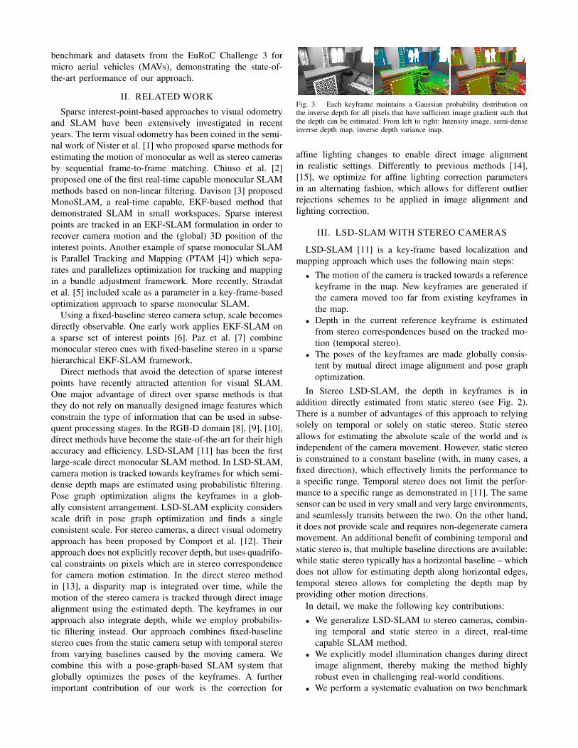
Take New KF?

Refine KFCreate New KF

Tracking Depth Map Estimation Map Optimization

CurrentMap

Add KF to MapTrack on Current KF

KFCurrentFrame

New Stereo Frame

NewKF

OldKF KF

CurrentFrame

track

propagate depth

staticstereo

CurrentKey Frame

temporal stereo

static stereo

align

alignCurrent KF

Fig. 2. Overview on the Stereo LSD-SLAM system.

datasets from realistic robotics applications, demonstrat-ing the state-of-the-art performance of our approach.

A. Notation

We use bold capital letters for matrices (such as R) andbold lower case letter for vectors (such as ξ). The operator[·]n selects the n-th row of a matrix. Throughout the paperwe use d to denote the inverse of the depth z of a point, i.e.,d = z−1.

In Stereo LSD-SLAM, a map is maintained as a set ofkeyframes Ki =

I li , I

ri , Di, Vi

. Each keyframe consists of

the left and right image I l/ri : Ω → R of the stereo camera,an inverse depth map Di : ΩDi

→ R+ and its variance mapVi : ΩDi → R+. Depth and variance are only maintainedfor one of the images in the stereo pair, we always use theleft image as reference frame. We assume the image domainΩ ⊂ R2 to be given in stereo-rectified image coordinates,i.e., the intrinsic and extrinsic camera parameters are knowna-priori. The domain ΩDi

⊂ Ω is the semi-dense restrictionto the pixels which are selected for depth estimation.

We denote pixel coordinates by u = (ux uy 1)T . A 3D

position p = (px py pz 1)T is projected into the image plane

through the mapping u = π(p) := K ((px/pz) (py/pz) 1)T ,

where K is the camera matrix. The mapping p =

π−1(u, d) :=((d−1K−1u

)T1)T

inverts the projectionwith the inverse depth d.

B. Depth Estimation

We estimate the geometry of the scene in keyframes. Eachkeyframe maintains Gaussian probability distributions on theinverse depth of a subset of pixels. This subset is chosenas the pixels with high image gradient magnitude, sincethese pixels provide rich structural information and morerobust disparity estimates than pixels in textureless areas.Figure 3 shows an example of such a semi-dense depthmap and associated variance map. We initialize the depthmap by propagating depth hypothesis from the previouskeyframe. The depth map is subsequently updated with newobservations in a pixel-wise depth-filtering framework. Wealso regularize the depth maps spatially and remove outliers.

In contrast to monocular SLAM, depth is estimated bothfrom static stereo (i.e., using images from different physical

cameras, but taken at the same point in time) as well as fromtemporal stereo (i.e., using images from the same physicalcamera, taken at different points in time).

a) Static Stereo: We determine the static stereo dispar-ity at a pixel by a correspondence search along its epipolarline in the other stereo image. In our case of stereo-rectifiedimages, this search can be performed very efficiently alonghorizontal lines.

As correspondence measure we use the SSD photometricerror over five pixels along the scanline. After subpixelaccurate refinement of the disparity, its variance is estimatedthrough the geometric and photometric error identified in[16]. If a Gaussian prior with mean d and standard de-viation σd on the inverse depth is available, we constrainthe search to [d− 2σd, d+ 2σd]. In practice, the searchinterval consists of only very few pixels for all but newlyinitialized hypothesis, greatly accelerating the search andreducing the probability of finding an incorrect or ambiguousmatch. According to the two error sources, we expect thatpixels with image gradients close to vertical, or with lowimage gradient along the horizontal direction do not provideaccurate disparity estimates. Hence, we neglect these pixelsfor static stereo.

When a new keyframe is initialized, we immediatelyperform static stereo to update and prune the propagateddepth map. In particular, pruning removes pixels that be-came occluded, and we fill in holes arising from forward-warping the depth map. Subsequently, we also make use ofstatic stereo from tracked non-keyframes, and integrate theobtained disparity information into the keyframe they weretracked on: In a first step, the inverse depth hypothesis at apixel u in the keyframe is transformed into the new frame,

u′ = π(Tξπ

−1 (u, d))

(1)

d′ =[Tξπ

−1 (u, d)]−1

3(2)

σ2d′ =

(d

d′

)4

σ2d, (3)

according to the pose estimate ξ. The propagated hypothesisis used as prior for a stereo search, and the respectiveobserved depth d′obs and observation variance σ2

d′,obs isdetermined. Finally, the observation is transformed back into

Fig. 4. Temporal vs. Static Stereo: Example of a scene where both temporalstereo (epipolar lines are parallel to the lane-markings on the road) andstatic stereo (epipolar lines are parallel to the horizontal bridge) alone failto capture all information present. Our combined approach fuses informationfrom both, and hence can reconstruct everything in the scene.

the keyframe using

dobs =[T−1ξ (π−1 (u′, d′obs))

]−1

3(4)

σ2obs =

(d′obs

dobs

)4

σ2d′,obs, (5)

and fused into the depth map. Note that observations fromnon-keyframes can only be generated for pixels with anexisting prior hypothesis – new hypothesis are only generatedduring stereo on the keyframe, or from temporal stereo. Thisprocess is schematically shown in Fig. 2.

b) Temporal Stereo: After tracking, we estimate dispar-ity between the current frame and the reference keyframe andfuse it in the keyframe. Again, we only use pixels for whichthe expected inverse depth error is sufficiently small. Wedetermine this uncertainty from several criteria: the imagegradient should be sufficiently large, not be parallel to theepipolar line and the pixel should not be close to the epipole.We kindly refer to [16] for further details on this method.While we use a simple 5-pixel SSD error, we correct foraffine lighting changes with the affine mapping found duringtracking, as will be described in Sec. III-C. Note that fortemporal stereo, the geometric error typically is higher thanfor static stereo, as relative camera pose stems from directimage alignment. This pose estimate often is less accuratethan the offline calibrated extrinsic calibration between thestereo camera pair.

C. Direct Image Alignment with Affine Lighting Correction

We determine the camera motion between two imagesusing direct image alignment. We use this method to trackcamera motion towards a reference keyframe. It is also usedfor estimating relative pose constraints between keyframesfor pose graph optimization. Finally, we propose a robustmethod to compensate for affine lighting changes.

1) Direct Image Alignment: The relative pose betweentwo images I l1 and I l2 is estimated by minimizing thephotometric residuals

rIu(ξ) := I l1 (u)− I l2 (π (p′)) (6)

where p′ := Tξπ−1 (u, D1(u)) and ξ transforms from

image frame I l2 to I l1. We also determine the uncertainty σIr,u

of this residual [11]. The optimization objective for trackinga current frame towards a keyframe is

Etrack(ξ) :=∑

u∈ΩD1

ρ

(rIu(ξ)

σIr,u

), (7)

where ρ is a robust weighting function; we choose ρ as theHuber norm. Note that in contrast to [12], we only align I l1 toI l2. While one could choose to add photometric constraints tothe new right image Ir2 , we observed that this can decreaseaccuracy in practice: typically, the baseline from I l1 to Ir2is much larger than to I l2, leading to more outliers fromocclusions and reflections.

Since fused depth is available in keyframes, we addgeometric residuals for keyframe-to-keyframe alignment,

rDu (ξ) := [p′]3 −D2 (π (p′)) (8)

providing additional information that is not available wheninitially tracking new frames, since these not have associateddepth estimates yet. The combined objective is

Ekeyframes(ξ) :=∑

u∈ΩD1

[ρ

(rIu(ξ)

σIr,u

)+ ρ

(rDu (ξ)

σDr,u

)](9)

Note that this formulation exploits the full depth informationavailable for both frames, including propagated and fusedobservations from other stereo pairs (see Sec. III-B). Thisis in contrast to an implicit quadrifocal approach as e.g. in[12].

We minimize these objectives using the iterativelyre-weighted Levenberg-Marquardt algorithm in a left-compositional formulation: Starting with an initial estimateξ(0), in each iteration a left-multiplied increment δξ(n) iscomputed by solving for the minimum of a second-orderapproximation of E, with fixed weights:

δξ(n) = −(JTWJ + λdiag(JTWJ))−1JTWr (10)

where

J =∂r(ε ξ(n))

∂ε

∣∣∣∣ε=0

(11)

is the derivative of the stacked vector of residuals r(ξ)with respect to a left-multiplied increment ε, JTWJ theGauss-Newton approximation of the Hessian of E, and Wa diagonal matrix containing the weights. The new estimateis then obtained by multiplication with the computed update

ξ(n+1) = δξ(n) ξ(n). (12)

We use a coarse-to-fine scheme to improve efficiency andbasin of convergence of the optimization.

Assuming the residuals to be statistically independent, theinverse of the Hessian from the last iteration (JTWJ)−1

is an estimate for the covariance Σξ of a left-multipliedincrement ε onto the final minimum, that is

ξ(n) = ε ξtrue with ε ∼ N (0,Σξ). (13)

In practice, the residuals are highly correlated, such that Σξis only a lower bound - yet it contains valuable informationabout the correlation between noise on the different degreesof freedom.

I1(u)

I2(u′)

I1(u)

I2(u′)

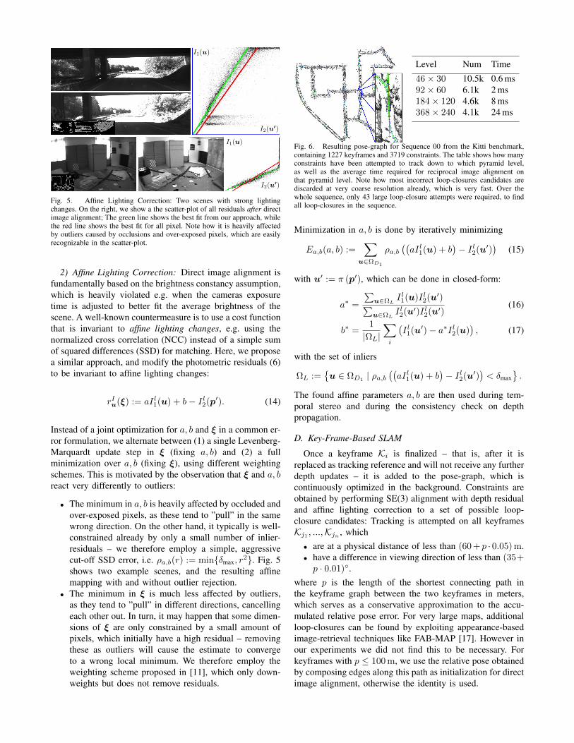
Fig. 5. Affine Lighting Correction: Two scenes with strong lightingchanges. On the right, we show a the scatter-plot of all residuals after directimage alignment; The green line shows the best fit from our approach, whilethe red line shows the best fit for all pixel. Note how it is heavily affectedby outliers caused by occlusions and over-exposed pixels, which are easilyrecognizable in the scatter-plot.

2) Affine Lighting Correction: Direct image alignment isfundamentally based on the brightness constancy assumption,which is heavily violated e.g. when the cameras exposuretime is adjusted to better fit the average brightness of thescene. A well-known countermeasure is to use a cost functionthat is invariant to affine lighting changes, e.g. using thenormalized cross correlation (NCC) instead of a simple sumof squared differences (SSD) for matching. Here, we proposea similar approach, and modify the photometric residuals (6)to be invariant to affine lighting changes:

rIu(ξ) := aI l1(u) + b− I l2(p′). (14)

Instead of a joint optimization for a, b and ξ in a common er-ror formulation, we alternate between (1) a single Levenberg-Marquardt update step in ξ (fixing a, b) and (2) a fullminimization over a, b (fixing ξ), using different weightingschemes. This is motivated by the observation that ξ and a, breact very differently to outliers:

• The minimum in a, b is heavily affected by occluded andover-exposed pixels, as these tend to ”pull” in the samewrong direction. On the other hand, it typically is well-constrained already by only a small number of inlier-residuals – we therefore employ a simple, aggressivecut-off SSD error, i.e. ρa,b(r) := minδmax, r

2. Fig. 5shows two example scenes, and the resulting affinemapping with and without outlier rejection.

• The minimum in ξ is much less affected by outliers,as they tend to ”pull” in different directions, cancellingeach other out. In turn, it may happen that some dimen-sions of ξ are only constrained by a small amount ofpixels, which initially have a high residual – removingthese as outliers will cause the estimate to convergeto a wrong local minimum. We therefore employ theweighting scheme proposed in [11], which only down-weights but does not remove residuals.

Level Num Time

46× 30 10.5k 0.6 ms92× 60 6.1k 2 ms184× 120 4.6k 8 ms368× 240 4.1k 24 ms

Fig. 6. Resulting pose-graph for Sequence 00 from the Kitti benchmark,containing 1227 keyframes and 3719 constraints. The table shows how manyconstraints have been attempted to track down to which pyramid level,as well as the average time required for reciprocal image alignment onthat pyramid level. Note how most incorrect loop-closures candidates arediscarded at very coarse resolution already, which is very fast. Over thewhole sequence, only 43 large loop-closure attempts were required, to findall loop-closures in the sequence.

Minimization in a, b is done by iteratively minimizing

Ea,b(a, b) :=∑

u∈ΩD1

ρa,b((aI l1(u) + b

)− I l2(u′)

)(15)

with u′ := π (p′), which can be done in closed-form:

a∗ =

∑u∈ΩL

I l1(u)I l2(u′)∑u∈ΩL

I l2(u′)I l2(u′)(16)

b∗ =1

|ΩL|∑i

(I l1(u′)− a∗I l2(u)

), (17)

with the set of inliers

ΩL :=u ∈ ΩD1

| ρa,b((aI l1(u) + b

)− I l2(u′)

)< δmax

.

The found affine parameters a, b are then used during tem-poral stereo and during the consistency check on depthpropagation.

D. Key-Frame-Based SLAM

Once a keyframe Ki is finalized – that is, after it isreplaced as tracking reference and will not receive any furtherdepth updates – it is added to the pose-graph, which iscontinuously optimized in the background. Constraints areobtained by performing SE(3) alignment with depth residualand affine lighting correction to a set of possible loop-closure candidates: Tracking is attempted on all keyframesKj1 , ...,Kjn , which• are at a physical distance of less than (60 + p · 0.05) m.• have a difference in viewing direction of less than (35+p · 0.01).

where p is the length of the shortest connecting path inthe keyframe graph between the two keyframes in meters,which serves as a conservative approximation to the accu-mulated relative pose error. For very large maps, additionalloop-closures can be found by exploiting appearance-basedimage-retrieval techniques like FAB-MAP [17]. However inour experiments we did not find this to be necessary. Forkeyframes with p ≤ 100 m, we use the relative pose obtainedby composing edges along this path as initialization for directimage alignment, otherwise the identity is used.

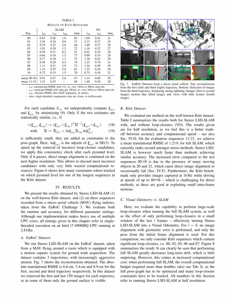
TABLE IRESULTS ON KITTI BENCHARK

SLAM VOSeq. trel rrel tabs time trel rrel time

00 0.63 0.26 1.0 82 1.09 0.42 2101 2.36 0.36 9.0 37 2.13 0.37 2402 0.79 0.23 2.6 64 1.09 0.37 2803 1.01 0.28 1.2 72 1.16 0.32 2704 0.38 0.31 0.2 51 0.42 0.34 2805 0.64 0.18 1.5 77 0.90 0.34 2906 0.71 0.18 1.3 72 1.28 0.43 2907 0.56 0.29 0.5 74 1.25 0.79 3108 1.11 0.31 3.9 73 1.24 0.38 2909 1.14 0.25 5.6 61 1.22 0.28 3010 0.72 0.33 1.5 70 0.75 0.34 21

mean 00-10 0.91 0.27 2.6 67 1.14 0.40 29mean 11-21 1.21 0.35 – 69 1.40 0.36 28

· trel: translational RMSE drift (%), av. over 100 m to 800 m intervals.· rrel: rotational RMSE drift (deg per 100 m), av. over 100 m to 800 m intervals.· tabs: absolute RMSE after 6DoF alignment, in meters.· time: single-threaded computation time per frame, in milliseconds.

For each candidate Kjk we independently compute ξjkiand ξijk by minimizing (9). Only if the two estimates arestatistically similar, i.e., if

e(ξjki, ξijk) := (ξjki ξijk)TΣ−1(ξjki ξijk) (18)

with Σ := Σjki + AdjjkiΣijkAdjTjki (19)

is sufficiently small, they are added as constraints to thepose-graph. Here, Adjjki is the adjoint of ξjki in SE(3). Tospeed up the removal of incorrect loop-closure candidates,we apply this consistency check after each pyramid level.Only if it passes, direct image alignment is continued on thenext higher resolution. This allows to discard most incorrectcandidates with only very little wasted computational re-sources: Figure 6 shows how many constraints where trackedon which pyramid level for one of the longest sequences inthe Kitti dataset.

IV. RESULTS

We present the results obtained by Stereo LSD-SLAM (1)on the well-known Kitti dataset, and (2) on three sequencesrecorded from a micro aerial vehicle (MAV) flying indoors,taken from the EuRoC Challenge 3. We evaluate boththe runtime and accuracy, for different parameter settings.Although our implementation makes heavy use of multipleCPU cores, all timings given in this chapter refer to single-threaded execution on an Intel i7-4900MQ CPU running at2.8 Ghz.

A. EuRoC Dataset

We run Stereo LSD-SLAM on the EuRoC dataset, takenfrom a MAV flying around a room which is equipped witha motion capture system for ground truth acquisition. Thedataset contains 3 trajectories, with increasingly aggressivemotion. Fig. 7 shows the reconstruction obtained. The abso-lute translational RMSE is 6.6 cm, 7.4 cm and 8.9 cm for thefirst, second and third trajectory respectively. In this datasetwe removed the first and last 150 images for each trajectory,as in some of them only the ground surface is visible.

Fig. 7. EuRoC Datasets from a micro aerial vehicle. Top: reconstructionfrom the first (left) and third (right) trajectory. Bottom: Selection of imagesfrom the third trajectory, displaying strong lightning changes (first to secondimage), motion blur (third image) and views with little texture (fourthimage).

B. Kitti Dataset

We evaluated our method on the well-known Kitti dataset.Table I summarizes the results both for Stereo LSD-SLAMwith, and without loop-closures (VO). The results givenare for half resolution, as we feel this is a better trade-off between accuracy and computational speed – see alsoSec. IV-D. On the evaluation sequences 11-21, we achievea mean translational RMSE of 1.21% for full SLAM, whichcurrently ranks second amongst stereo methods. Stereo LSD-SLAM is however much faster than methods achievingsimilar accuracy. The increased error compared to the testsequences 00-10 is due to the presence of many movingobjects in 20 and 21, which cause direct image alignment tooccasionally fail (Sec. IV-F). Furthermore, the Kitti bench-mark only provides images captured at 10 Hz while drivingat speeds of up to 80 km/h – which is challenging for directmethods, as these are good at exploiting small intra-framemotions.

C. Visual Odometry vs. SLAM

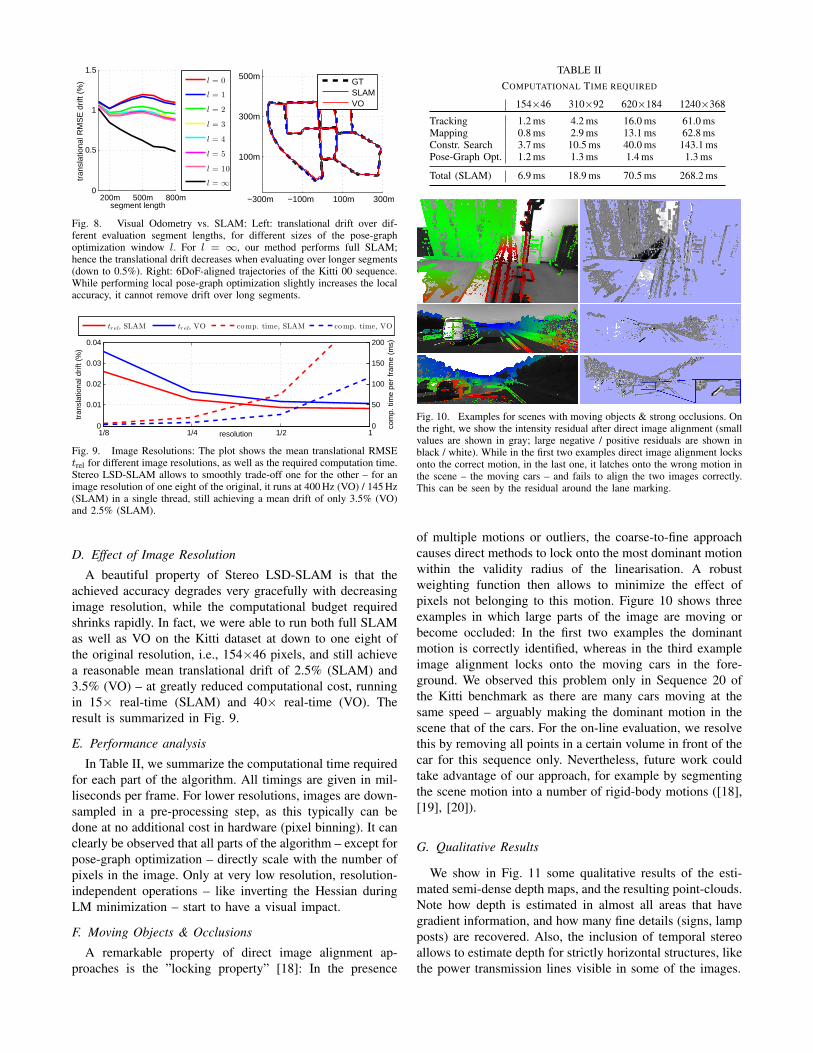
Here, we evaluate the capability to perform large-scaleloop-closures when running the full SLAM system, as wellas the effect of only performing loop-closures in a smallwindow of the last l frames – effectively turning StereoLSD-SLAM into a Visual Odometry. For l = 0, no imagealignment with geometric error is performed, and only thepose from the initial frame alignment is used. For thiscomparison, we only consider Kitti sequences which containsignificant loop-closures, i.e. 00, 02, 05, 06 and 07. Figure 8summarizes the result: It can clearly be seen that performingfull SLAM greatly decreases long-term drift, which is littlesurprising. However, this comes at increased computationalcost: when performing full SLAM, the overall computationalbudget required more than doubles (also see Tab. I), as thefull pose-graph has to be optimized and many loop-closureconstraints have to be tracked. All numbers in this Sectionrefer to running Stereo LSD-SLAM at half resolution.

200m 500m 800m0

0.5

1

1.5

segment length

tran

slat

iona

l RM

SE

drif

t (%

)

l = 0

l = 1

l = 2

l = 3

l = 4

l = 5

l = 10

l = ∞

−300m −100m 100m 300m

100m

300m

500m

GTSLAMVO

Fig. 8. Visual Odometry vs. SLAM: Left: translational drift over dif-ferent evaluation segment lengths, for different sizes of the pose-graphoptimization window l. For l = ∞, our method performs full SLAM;hence the translational drift decreases when evaluating over longer segments(down to 0.5%). Right: 6DoF-aligned trajectories of the Kitti 00 sequence.While performing local pose-graph optimization slightly increases the localaccuracy, it cannot remove drift over long segments.

1/8 1/4 1/2 1 0

0.01

0.02

0.03

0.04

tran

slat

iona

l drif

t (%

)

0

50

100

150

200

com

p. ti

me

per

fram

e (m

s)

resolution

trel, SLAM trel, VO comp. time, SLAM comp. time, VO

Fig. 9. Image Resolutions: The plot shows the mean translational RMSEtrel for different image resolutions, as well as the required computation time.Stereo LSD-SLAM allows to smoothly trade-off one for the other – for animage resolution of one eight of the original, it runs at 400 Hz (VO) / 145 Hz(SLAM) in a single thread, still achieving a mean drift of only 3.5% (VO)and 2.5% (SLAM).

D. Effect of Image Resolution

A beautiful property of Stereo LSD-SLAM is that theachieved accuracy degrades very gracefully with decreasingimage resolution, while the computational budget requiredshrinks rapidly. In fact, we were able to run both full SLAMas well as VO on the Kitti dataset at down to one eight ofthe original resolution, i.e., 154×46 pixels, and still achievea reasonable mean translational drift of 2.5% (SLAM) and3.5% (VO) – at greatly reduced computational cost, runningin 15× real-time (SLAM) and 40× real-time (VO). Theresult is summarized in Fig. 9.

E. Performance analysis

In Table II, we summarize the computational time requiredfor each part of the algorithm. All timings are given in mil-liseconds per frame. For lower resolutions, images are down-sampled in a pre-processing step, as this typically can bedone at no additional cost in hardware (pixel binning). It canclearly be observed that all parts of the algorithm – except forpose-graph optimization – directly scale with the number ofpixels in the image. Only at very low resolution, resolution-independent operations – like inverting the Hessian duringLM minimization – start to have a visual impact.

F. Moving Objects & Occlusions

A remarkable property of direct image alignment ap-proaches is the ”locking property” [18]: In the presence

TABLE IICOMPUTATIONAL TIME REQUIRED

154×46 310×92 620×184 1240×368

Tracking 1.2 ms 4.2 ms 16.0 ms 61.0 msMapping 0.8 ms 2.9 ms 13.1 ms 62.8 msConstr. Search 3.7 ms 10.5 ms 40.0 ms 143.1 msPose-Graph Opt. 1.2 ms 1.3 ms 1.4 ms 1.3 ms

Total (SLAM) 6.9 ms 18.9 ms 70.5 ms 268.2 ms

Fig. 10. Examples for scenes with moving objects & strong occlusions. Onthe right, we show the intensity residual after direct image alignment (smallvalues are shown in gray; large negative / positive residuals are shown inblack / white). While in the first two examples direct image alignment locksonto the correct motion, in the last one, it latches onto the wrong motion inthe scene – the moving cars – and fails to align the two images correctly.This can be seen by the residual around the lane marking.

of multiple motions or outliers, the coarse-to-fine approachcauses direct methods to lock onto the most dominant motionwithin the validity radius of the linearisation. A robustweighting function then allows to minimize the effect ofpixels not belonging to this motion. Figure 10 shows threeexamples in which large parts of the image are moving orbecome occluded: In the first two examples the dominantmotion is correctly identified, whereas in the third exampleimage alignment locks onto the moving cars in the fore-ground. We observed this problem only in Sequence 20 ofthe Kitti benchmark as there are many cars moving at thesame speed – arguably making the dominant motion in thescene that of the cars. For the on-line evaluation, we resolvethis by removing all points in a certain volume in front of thecar for this sequence only. Nevertheless, future work couldtake advantage of our approach, for example by segmentingthe scene motion into a number of rigid-body motions ([18],[19], [20]).

G. Qualitative Results

We show in Fig. 11 some qualitative results of the esti-mated semi-dense depth maps, and the resulting point-clouds.Note how depth is estimated in almost all areas that havegradient information, and how many fine details (signs, lampposts) are recovered. Also, the inclusion of temporal stereoallows to estimate depth for strictly horizontal structures, likethe power transmission lines visible in some of the images.

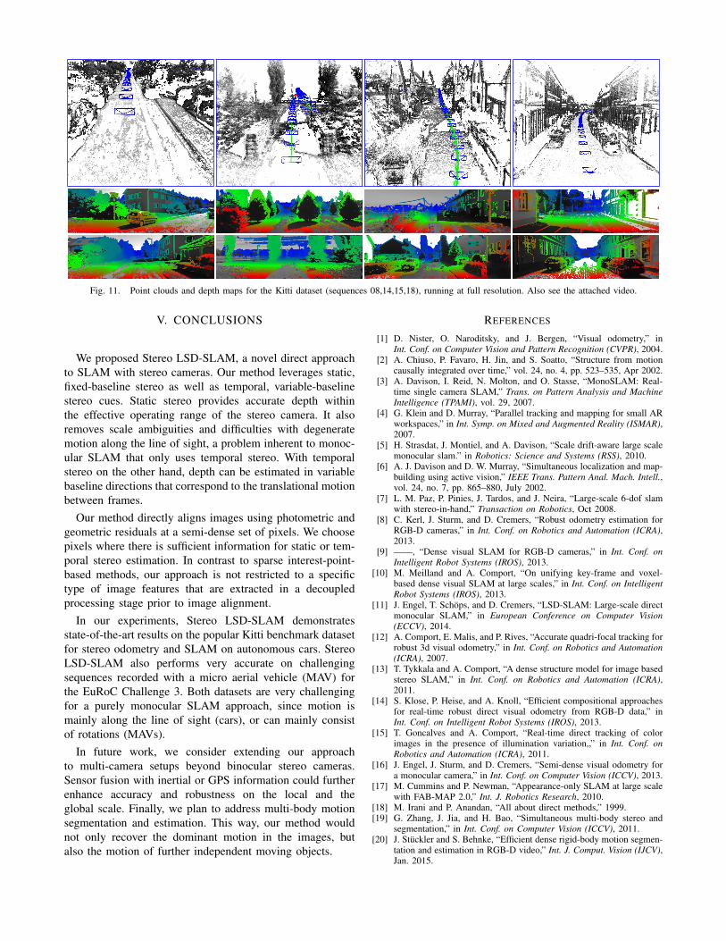
Fig. 11. Point clouds and depth maps for the Kitti dataset (sequences 08,14,15,18), running at full resolution. Also see the attached video.

V. CONCLUSIONS

We proposed Stereo LSD-SLAM, a novel direct approachto SLAM with stereo cameras. Our method leverages static,fixed-baseline stereo as well as temporal, variable-baselinestereo cues. Static stereo provides accurate depth withinthe effective operating range of the stereo camera. It alsoremoves scale ambiguities and difficulties with degeneratemotion along the line of sight, a problem inherent to monoc-ular SLAM that only uses temporal stereo. With temporalstereo on the other hand, depth can be estimated in variablebaseline directions that correspond to the translational motionbetween frames.

Our method directly aligns images using photometric andgeometric residuals at a semi-dense set of pixels. We choosepixels where there is sufficient information for static or tem-poral stereo estimation. In contrast to sparse interest-point-based methods, our approach is not restricted to a specifictype of image features that are extracted in a decoupledprocessing stage prior to image alignment.

In our experiments, Stereo LSD-SLAM demonstratesstate-of-the-art results on the popular Kitti benchmark datasetfor stereo odometry and SLAM on autonomous cars. StereoLSD-SLAM also performs very accurate on challengingsequences recorded with a micro aerial vehicle (MAV) forthe EuRoC Challenge 3. Both datasets are very challengingfor a purely monocular SLAM approach, since motion ismainly along the line of sight (cars), or can mainly consistof rotations (MAVs).

In future work, we consider extending our approachto multi-camera setups beyond binocular stereo cameras.Sensor fusion with inertial or GPS information could furtherenhance accuracy and robustness on the local and theglobal scale. Finally, we plan to address multi-body motionsegmentation and estimation. This way, our method wouldnot only recover the dominant motion in the images, butalso the motion of further independent moving objects.

REFERENCES

[1] D. Nister, O. Naroditsky, and J. Bergen, “Visual odometry,” inInt. Conf. on Computer Vision and Pattern Recognition (CVPR), 2004.

[2] A. Chiuso, P. Favaro, H. Jin, and S. Soatto, “Structure from motioncausally integrated over time,” vol. 24, no. 4, pp. 523–535, Apr 2002.

[3] A. Davison, I. Reid, N. Molton, and O. Stasse, “MonoSLAM: Real-time single camera SLAM,” Trans. on Pattern Analysis and MachineIntelligence (TPAMI), vol. 29, 2007.

[4] G. Klein and D. Murray, “Parallel tracking and mapping for small ARworkspaces,” in Int. Symp. on Mixed and Augmented Reality (ISMAR),2007.

[5] H. Strasdat, J. Montiel, and A. Davison, “Scale drift-aware large scalemonocular slam.” in Robotics: Science and Systems (RSS), 2010.

[6] A. J. Davison and D. W. Murray, “Simultaneous localization and map-building using active vision,” IEEE Trans. Pattern Anal. Mach. Intell.,vol. 24, no. 7, pp. 865–880, July 2002.

[7] L. M. Paz, P. Pinies, J. Tardos, and J. Neira, “Large-scale 6-dof slamwith stereo-in-hand,” Transaction on Robotics, Oct 2008.

[8] C. Kerl, J. Sturm, and D. Cremers, “Robust odometry estimation forRGB-D cameras,” in Int. Conf. on Robotics and Automation (ICRA),2013.

[9] ——, “Dense visual SLAM for RGB-D cameras,” in Int. Conf. onIntelligent Robot Systems (IROS), 2013.

[10] M. Meilland and A. Comport, “On unifying key-frame and voxel-based dense visual SLAM at large scales,” in Int. Conf. on IntelligentRobot Systems (IROS), 2013.

[11] J. Engel, T. Schops, and D. Cremers, “LSD-SLAM: Large-scale directmonocular SLAM,” in European Conference on Computer Vision(ECCV), 2014.

[12] A. Comport, E. Malis, and P. Rives, “Accurate quadri-focal tracking forrobust 3d visual odometry,” in Int. Conf. on Robotics and Automation(ICRA), 2007.

[13] T. Tykkala and A. Comport, “A dense structure model for image basedstereo SLAM,” in Int. Conf. on Robotics and Automation (ICRA),2011.

[14] S. Klose, P. Heise, and A. Knoll, “Efficient compositional approachesfor real-time robust direct visual odometry from RGB-D data,” inInt. Conf. on Intelligent Robot Systems (IROS), 2013.

[15] T. Goncalves and A. Comport, “Real-time direct tracking of colorimages in the presence of illumination variation,,” in Int. Conf. onRobotics and Automation (ICRA), 2011.

[16] J. Engel, J. Sturm, and D. Cremers, “Semi-dense visual odometry fora monocular camera,” in Int. Conf. on Computer Vision (ICCV), 2013.

[17] M. Cummins and P. Newman, “Appearance-only SLAM at large scalewith FAB-MAP 2.0,” Int. J. Robotics Research, 2010.

[18] M. Irani and P. Anandan, “All about direct methods,” 1999.[19] G. Zhang, J. Jia, and H. Bao, “Simultaneous multi-body stereo and

segmentation,” in Int. Conf. on Computer Vision (ICCV), 2011.[20] J. Stuckler and S. Behnke, “Efficient dense rigid-body motion segmen-

tation and estimation in RGB-D video,” Int. J. Comput. Vision (IJCV),Jan. 2015.