161

Reihe Ökonomie

Economics Series

Imports, Status Preference, and Foreign Borrowing

Walter H. Fisher

161

Reihe Ökonomie

Economics Series

Imports, Status Preference, and Foreign Borrowing

Walter H. Fisher

September 2004

Institut für Höhere Studien (IHS), Wien Institute for Advanced Studies, Vienna

Contact: Walter H. Fisher Department of Economics and Finance Institute for Advanced Studies Stumpergasse 56, 1060 Vienna

: +43/1/599 91-253 email: fisher@ihs.ac.at

Founded in 1963 by two prominent Austrians living in exile – the sociologist Paul F. Lazarsfeld and the economist Oskar Morgenstern – with the financial support from the Ford Foundation, the AustrianFederal Ministry of Education and the City of Vienna, the Institute for Advanced Studies (IHS) is the first institution for postgraduate education and research in economics and the social sciences in Austria.The Economics Series presents research done at the Department of Economics and Finance andaims to share “work in progress” in a timely way before formal publication. As usual, authors bear fullresponsibility for the content of their contributions. Das Institut für Höhere Studien (IHS) wurde im Jahr 1963 von zwei prominenten Exilösterreichern –dem Soziologen Paul F. Lazarsfeld und dem Ökonomen Oskar Morgenstern – mit Hilfe der Ford-Stiftung, des Österreichischen Bundesministeriums für Unterricht und der Stadt Wien gegründet und istsomit die erste nachuniversitäre Lehr- und Forschungsstätte für die Sozial- und Wirtschafts-wissenschaften in Österreich. Die Reihe Ökonomie bietet Einblick in die Forschungsarbeit der Abteilung für Ökonomie und Finanzwirtschaft und verfolgt das Ziel, abteilungsinterneDiskussionsbeiträge einer breiteren fachinternen Öffentlichkeit zugänglich zu machen. Die inhaltliche Verantwortung für die veröffentlichten Beiträge liegt bei den Autoren und Autorinnen.

Abstract

This paper considers the implications of consumption and borrowing externalities in a small open economy framework. The former reflect the assumption that status conscious agents care about the relative consumption of imported goods, while the latter arise because agents do not take into account the effects of their borrowing decisions on the interest rate on debt. We analyze in the paper the impact of an increase in the degree of status preference on the saddlepath adjustment of the decentralized economy. In addition, the contrasting steady-state and dynamic properties of the social planner's economy are derived, along with the corresponding optimal tax and subsidy policies.

Keywords Imports, status-preference, current account dynamics

JEL Classification E21, F41

Comments I wish to thank Franz X. Hof for his valuable advice and assistance and the Jubilaeumsfonds of theOesterreichische Nationalbank (OeNB), Project No. 8701, for its generous financial support.

Contents

1. Introduction 1

2. The Model and Intertemporal Equilibrium 4

3. Dynamics of an Increase in Status Preference 12 3.1. Long-Run Responses .............................................................................................. 12 3.2. Transitional Dynamics.............................................................................................. 13

4. The Planner's Problem and Optimal Taxation 16 4.1. Intertemporal Equilibrium ......................................................................................... 16 4.2. Optimal Policy .......................................................................................................... 23

5. Conclusions 24

6. Appendix 25 6.1. Partial Derivatives in (2.8a)–(2.8d) ......................................................................... 25 6.2. Expressions for the Long-Run Comparative Statistics ............................................ 26 6.3. Expression for the Trade Balance ........................................................................... 27 6.4. Expressions for rb and rd .......................................................................................... 27 6.5. Partial Derivatives of (4.3a)–(4.3d) ......................................................................... 28 6.6. Expressions for the Deviations of Decentralized Variables from

Their Social Optima ................................................................................................ 29 6.7. Solution for the Trade Balance in the Social Optimum ........................................... 31

References 31

Figures 34

1. Introduction

One measure of an economys Þnancial market integration is the terms at which it can borrow

in international capital markets. According to a basic deÞnition, a country may be perfectly

integrated if it can borrow (and lend) at the prevailing world interest rate, however the latter

is speciÞed. Due, however, to factors such as default risk, a developing economy may be subject

to an external constraint that regulates the terms at which it borrows from abroad. A way

of capturing this idea in a reduced-form framework is to specify that the interest rate on debt

depends on a countrys ability to service its existing level of international obligations. This leads

to an upward-sloping interest rate relationship in which the rate on debt rises with the level

of indebtedness, where the latter can be scaled by a measure, such as GDP, of the economys

ability to pay. An early use of this idea was employed by Bardhan (1967) and has, more recently,

been taken up by researchers such as Pitchford (1989), Bhandari et. al. (1990), Fisher (1995),

Agenor (1998), Fisher and Terrell (2000), and Chatterjee and Turnovsky (2004), all of whom

use the representative agent framework. These authors employ this relationship to study the

intertemporal impact of macroeconomic disturbances, such as domestic Þscal policy and world

interest rate shocks, on indebted open economies

In analyzing economies with this type of interest rate function, an important feature is

whether or not agents take into account the upward-sloping nature of the relationship; in

other words, whether or not agents recognize that their borrowing decisions affect the equilibrium

interest rate on debt instruments. The models of Pitchford (1989), Bhandari et al. (1990), and

Agenor (1998) specify that agents do recognize the fact that greater foreign borrowing raises the

interest rate on debt, while the work of Fisher (1995), Fisher and Terrell (2000), and Chatterjee

and Turnovsky (2004) assumes, on the other hand, that agents take the interest rate on debt as

given in making their optimal choices. The latter formulation can be interpreted as a model of

sovereign debt, with the interest rate relationship incorporating a country speciÞc interest cost

function that is rising (and convex) in a measure of the economys indebtedness.1 Nevertheless,

as Pitchford (1989), among others, points out, the country speciÞc speciÞcation results in a

borrowing externality. While this externality is not (necessarily) crucial for the results of the

1Bhandari et. al. (1990) do, however, incorporate features of the sovereign debt model such shifts in the cost,or risk, premium.

1

work cited above, we show in our framework that it does play an important role in characterizing

the economys steady-state and saddlepath dynamics. Indeed, one of the goals of this paper is

to compare the dynamic properties of the two speciÞcations of borrowing behavior, which, in

certain respects, is more complex if these decisions are internalized.

A developing economy need not only be ridden with one externality, however. Indeed,

consumption and production externalities can also play a crucial role in inßuencing the evolution

of developing economies. In this paper we consider how consumption externalities affect an

economy subject to an external borrowing constraint. Consumption externalities arise in our

framework because we assume that agents gain utility not only from their individual consumption

of goods and services, but also from their relative social position, or status. Using survey data

suggesting that higher levels of average income do not necessarily translate into higher levels

of personal satisfaction, Easterlin (1974, 1995) and Oswald (1997) infer, in contrast, that social

position is a key factor in determining overall well-being.2

In our reduced-form speciÞcation of instantaneous preferences, social status is conferred by

relative consumption, so that the consumption externality in our model corresponds to the de-

veloping economys average, or aggregate, level of consumption. There is a growing literature

that investigates the inßuence of consumption externalities in dynamic macroeconomies. Repre-

sentative authors who considered this issue in the closed economy context include Galõ (1994),

Rauscher (1997), Grossmann (1998), Fisher and Hof (2000a, b), Dupor and Liu (2003), and

Liu and Turnovsky (2004).3 We extend this work by analyzing consumption externalities in the

case of a two-good, open economy, subject to an external borrowing constraint. SpeciÞcally, we

assume that it is the relative consumption of imported goods that confers social position, an

idea that is, we believe, plausible in the case of a developing economy where foreign luxuries

represent status goods.

2More general studies of the economic implications of the quest for social status are provided by Frank (1985)and Cole, Mailath, and Postlewaite (1992). To curtail potentially wasteful status competition, Frank (1997)advocates instituting a progressive consumption tax, implemented by exempting savings from taxation.

3An alternative branch of this line of research speciÞes that status depends on relative wealth, rather thanon relative consumption. Recent authors who have employed this approach include Corneo and Jeanne (1997),Futagami and Shibata (1998), and Fisher (2004). Fisher (2004) shows how relative wealth preferences can be usedto obtainin the context of the small open economy Ramsey model with perfect capital mobilityan interior,steady-state saddlepoint. General discussions of the problem of obtaining interior steady states in a small opencontext are found in Barro and Sala-i-Martin (1995), [ch. 3, pp. 101-25] and Turnovsky (1997), [ch. 2, pp. 36-47and ch. 3, pp. 57-77]. One way of dealing with this issue is to impose an external borrowing constraint, anapproach we adopt in this paper.

2

The basic framework we employ closely follows Fisher (1995): (i) the developing economy

is modelled as a representative consumer-producer who consumes a domestic goodproduced

using the single-factor laborand a good imported from abroad; (ii) the economy is semi-small

in the sense that it has an endogenous terms of trade (in goods) relative to the rest of the world;

and (iii) international borrowing is subject to an upward-sloping interest rate relationship that

depends on the stock of debt. We extend this framework, Þrst, by incorporating preferences that

are a function of the relative consumption of imported goods. Furthermore, in this paper we

modify the borrowing relationship by specifying that interest costs are a function of the debt

to GDP ratio. For convenience, we divide the exposition of the model into two parts: (i) the

decentralized framework that is subject to consumption externalities and in which agents take

the interest rate relationship as given; and (ii) the socially optimal framework, where the effects

of the consumption externality are eliminated and in which the planner internalizes the interest

costs of the economys borrowing decision. To derive a symmetric macroeconomic equilibrium

in the decentralized framework, we assume that all agents take the same actions, which is the

typical procedure in models of this type. Moreover, because the interest rate relationship in this

paper depends on the debt to GDP ratio, there is also, in effect, a production externality in the

decentralized equilibrium in addition to a borrowing externality.4

To investigate how the consumption externality interacts with the borrowing constraint, we

analyze how the economy responds over time to a permanent increase in the preference weight

on the relative consumption of imported goods. We show that this causes the economy in the

long-run to expand, i.e., due to higher work effort domestic output increases, which, in turn,

results in a decline in the countrys terms of trade and a corresponding rise in net exports.5 As

a consequence, the economy supports a higher steady-state stock of debt and consumes more of

the imported good (the long-run response of steady-state consumption is, however, ambiguous).

Using a standard phase diagram apparatus, we illustrate the transitional dynamics in response

to the increase in status preference. While we distinguish three separate cases, we demonstrate

that the transitional adjustment of the economy in all instances involves current account deÞcits,

4Likewise, the model of Liu and Turnovsky (2004) incorporates consumption and production externalities,although in their paper production externalities reßect spillovers from the aggregate capital stock.

5This result is consistent with the single-good, closed economy Þndings of Fisher and Hof (2000b) and Liu andTurnovsky (2004), who show that preferences for relative consumption (or the existence of negative consumptionexternalities) causes a rise in equilibrium employment relative to economies in which these motives are absent.

3

a deterioration in the terms of trade, and declines in the economys consumption of domestic and

foreign goods. In addition, the trade balance, after an initial fall, improves along the economys

saddlepath in order to support the long-run increase indebtedness. In this part of the paper we

also describe the behavior of the interest rate on debt and the economys domestic, internal

rate of return, the latter depending on the dynamics of the terms of trade.

The remainder of the paper is structured as follows: section 2 describes the modelling frame-

work and derives the circumstances in which the decentralized economy is characterized by

(local) saddlepoint dynamics. To study the interactions between borrowing and consumption

externalities, we consider in section 3 the intertemporal implications of a permanent increase

in the degree of status consciousness. Section 4 is devoted to analyzing the socially optimal

counterpart to the decentralized economy. In this section we analyze how the steady-state and

saddlepoint properties of the planners economy differ from those of its decentralized counter-

part and calculate the optimal tax and subsidy policies that reproduce the social optimum.

The paper closes with brief concluding remarks in section 5 and an appendix containing some

mathematical results.

2. The Model and Intertemporal Equilibrium

We introduce the model by assuming that there are a large number of representative agents, each

of whom has the following instantaneous preferences over their own consumption of domestic

and foreign goods, x and y, status, s, and work effort, l:6

W (x, y, s, l) ≡ U(x, y) + δs(y/Y ) + V (l), δ > 0. (2.1)

In this formulation, also employed by Rauscher (1997), Fisher and Hof (2000b), and Liu and

Turnovsky (2004), preferences over own consumption are additively separable from status. In

addition, both are separable from work effort. According to (2.1), status depends on the relative

consumption of foreign goods, y/Y , where Y denotes the aggregate, or average, level of imported

goods consumed by the small open economy and the parameter δ represents the corresponding

6All variables in the model are denominated in real terms.

4

utility weight.7 We further specify that W (x, y, s, l) has the following Þrst derivative and

curvature properties:8

Ux > 0, Uxx < 0, Uy > 0, Uyy < 0, Uxy > 0, UxxUyy − U2xy > 0,

s0 > 0, s00 < 0, Vl < 0, Vll < 0. (2.2)

The function U(x, y) obeys the standard assumptions that utility is increasing in the consump-

tion of own goods and strictly concave. The condition Uxy > 0 imposes Edgeworth comple-

mentarity on the own consumption of domestic and foreign goods. In addition, (2.2) implies

that status is increasing and concave in the relative consumption of imports, while work effort

generates disutility and is strictly concave.

Regarding agents production and Þnancial market possibilities, we assume, Þrst, that the

production of tradable output, q, depends on the single factor employment, l, which has the

standard properties of positive and declining marginal productivity: q = F (l), F 0 > 0, F 00 <

0.9 We specify next that the interest rate at which agents borrow dependsin addition to

the exogenous and time invariant world interest rateon the economys ability to service its

outstanding level of obligations, as measured by the debt to GDP ratio. Letting rb[b/F (l)]

represent the interest rate on foreign debt, this relationship is deÞned by the following equation

rb ≡ rb[b/F (l)] = r∗ + α[b/F (l)], α0 > 0, α00 > 0, (2.3)

where r∗ is the given world interest rate and α[b/F (l)] is the country-speciÞc interest cost,

which is a positive, increasing function of b/F (l), the ratio of outstanding debt to domestic

output.10 Equation (2.3) is in contrast to most of the work cited above that speciÞes α(·) asa function of b alone.11 The early study of Edwards (1984)showing a positive relationship

7Below, we employ a modiÞed version of δ, given by η ≡ δs0(1) > 0, where y ≡ Y in the symmetric equilibrium.8The following notational conventions are observed: partial derivatives of functions are denoted by subscripts;

derivatives of functions with a single argument are indicated by primes; and time derivatives are denoted bydots. In general, we suppress a variables time dependence.

9The implicit assumption of a Þxed domestic capital stock allows us to simplify the analysis, particularlythe derivation of the dynamic equilibrium, and to focus on some of the central implications of borrowing andconsumption externalities.

10We assume for expositional purposes that the country is always a net debtor, b > 0, although it is straight-forward to generalize the results to the case in which the country is a net creditor, b < 0.

11Exceptions are Bhandari et. al. (1990) and Chatterjee and Turnovsky (2004), who scale national indebtedness

5

between the interest rate spread over the LIBOR rate and the debt to GDP ratioprovides for

a set of developing economies some empirical evidence for (2.3). For our purposes, a further

crucial advantage of the debt to GDP speciÞcation in (2.3) is that shifts in status preference that

change the level of employment (and output) lead to a non-degenerate transitional dynamics,

which, on the other hand, do not occur if α(·) is a function of debt alone (see footnote 24 below).

In the context of a perfect foresight, dynamic equilibrium, the agents maximization problem

is formulated as follows

max

Z ∞

0[U(x, y) + s (y/Y ) + V (l)]e−ρtdt, (2.4a)

subject to

úb = y + [x− F (l)]/p+ rb[b/F (l)]b, b(0) = b0 > 0, (2.4b)

where ρ is the exogenous rate of pure time preference, p is the relative price of the foreign in

terms of the domestic good, and b0 is the inherited stock of debt.12 Observe that the ßow

constraint for the accumulation of debt is formulated in terms of the foreign good. In solving

the optimization problem, we posit that the agent takes the average consumption of imported

goods Y as given and ignores the effect of his work effort and borrowing decisions on the bond

rate rb.13 Applying standard optimizing techniques for this class of problem, the following Þrst

order conditions obtain

Ux (x, y) = λ/p, Uy (x, y) + Y−1δs0 (y/Y ) = λ, (2.5a, b)

V 0(l) = −λF 0(l)/p, úλ = λρ− rb[b/F (l)], (2.5c, d)

where λ the current costate variable, evaluated in terms of the foreign good. Equation (2.5a) is

the necessary condition for consumption of the domestic good, while (2.5b) is the corresponding

condition for imports. Observe that the marginal utility of imported goods is the sum of the

by the stock of physical capital.12Since p is the relative price in terms of the domestic good, a rise (resp. fall) in p corresponds to a fall (resp.

decline) in the economys terms of trade.13Since agents optimize holding rb constant, it is unnecessary to introduce the distinction between individual

and average levels of indebtedness. Also, as is usual in models of this type, the agent takes as given the terms oftrade p, although it is endogenous in equilibrium.

6

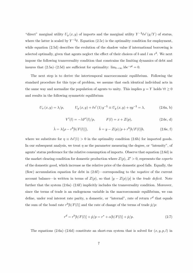
direct marginal utility Uy (x, y) of imports and the marginal utility Y−1δs0 (y/Y ) of status,

where the latter is scaled by Y −1δ. Equation (2.5c) is the optimality condition for employment,

while equation (2.5d) describes the evolution of the shadow value if international borrowing is

selected optimally, given that agents neglect the effect of their choices of b and l on rb. We next

impose the following transversality condition that constrains the limiting dynamics of debt and

insures that (2.5a)(2.5d) are sufficient for optimality: limt→∞ λbe−ρt = 0.

The next step is to derive the intertemporal macroeconomic equilibrium. Following the

standard procedure for this type of problem, we assume that each identical individual acts in

the same way and normalize the population of agents to unity. This implies y = Y holds ∀t ≥ 0and results in the following symmetric equilibrium

Ux (x, y) = λ/p, Uy (x, y) + δs0 (1) y−1 ≡ Uy (x, y) + ηy−1 = λ, (2.6a, b)

V 0(l) = −λF 0(l)/p, F (l) = x+ Z(p), (2.6c, d)

úλ = λρ− rb[b/F (l)], úb = y − Z(p)/p+ rb[b/F (l)]b, (2.6e, f)

where we substitute for η ≡ δs0(1) > 0 in the optimality condition (2.6b) for imported goods.In our subsequent analysis, we treat η as the parameter measuring the degree, or intensity, of

agents status preference for the relative consumption of imports. Observe that equation (2.6d) is

the market clearing condition for domestic production where Z(p), Z 0 > 0, represents the exports

of the domestic good, which increase as the relative price of the domestic good falls. Equally, the

(ßow) accumulation equation for debt in (2.6f)corresponding to the negative of the current

account balanceis written in terms of Z(p), so that [y − Z(p)/p] is the trade deÞcit. Notefurther that the system (2.6a)(2.6f) implicitly includes the transversality condition. Moreover,

since the terms of trade is an endogenous variable in the macroeconomic equilibrium, we can

deÞne, under real interest rate parity, a domestic, or internal, rate of return rd that equals

the sum of the bond rate rb[b/F (l)] and the rate of change of the terms of trade úp/p:

rd = rb[b/F (l)] + úp/p = r∗ + α[b/F (l)] + úp/p. (2.7)

The equations (2.6a)(2.6d) constitute an short-run system that is solved for (x, y, p, l) in

7

terms of the marginal utility of wealth λ and the status parameter η

x = x(λ, η), xλ < 0, xη > 0; y = y(λ, η), yλ < 0, yη > 0, (2.8a, b)

p = p(λ, η), pλ > 0, pη < 0; l = l(λ, η), lλ > 0, lη > 0, (2.8c, d)

where we indicate in (2.8a)(2.8d) the signs of the partial derivatives of the solutions (x, y, p, l)

with respect to λ and η.14 The actual expressions for the partial derivatives are stated in

the appendix [see (6.1a)(6.1d) and (6.2a)(6.2d)] and are interpreted as follows: a rise in the

shadow value λ lowers the consumption of domestic and foreign goods, x and y, and as well as

the consumption of leisure. The resulting increase in employment, l, and domestic output, q,

lowers, in turn, the relative price of domestic goods, i.e., p rises. In contrast, an increase in the

status preference parameter η increases the demand for imported goods y. Due the assumption

of Edgeworth complementarity (Uxy > 0), the higher value of η leads to an increase in the

consumption of domestic goods and leisure, i.e., both x and l rise. This, in turn, raises the

countrys terms of trade so that p falls.

Turning the economys dynamics, we obtain the differential equations describing the evo-

lution of the marginal utility of wealth and stock of debt by substituting the instantaneous

solutions (2.8b)(2.8d), together with the expression (2.3) for rb, into (2.6e)(2.6f):

úλ = λ

½ρ−

·r∗ + α

µb

F [l(λ, η)]

¶¸¾(2.9a)

úb = y (λ, η)− Z [p (λ, η)]p (λ, η)

+

½r∗ + α

·b

F [l(λ, η)]

¸¾b. (2.9b)

Letting úλ = úb = 0 in (2.9a, b), the corresponding steady-state equilibrium constitutes the

following set of relationships

Ux (x, y) = λ/p, Uy (x, y) + ηy−1 = λ, (2.10a, b)

V 0(l) = −λF 0(l)/p, F (l) = x+ Z(p), (2.10c, d)

14Although it is not the focus of the analysis, the equilibrium (2.8a)(2.8d) also depends on the parameters ofthe production and export functions.

8

rb = rb[b/F (l)] = r∗ + α[b/F (l)] = rd = ρ, (2.10e)

Z (p)− py = pr∗ + α[b/F (l)]b, (2.10f)

where the symbol indicates a long-run variable. Equations (2.10a)(2.10d) are the long-run

versions of (2.6a)(2.6d), while (2.10e) and (2.10f) state, respectively, that the long-run interest

rates rb and rd equal the exogenous rate of time preference ρ and that steady-state interest

servicein terms of the domestic goodequals the domestic trade balance (net exports).

Taking Þrst-order approximations of (2.9a, b) around the steady-state system (2.10a)(2.10f),

the following matrix differential equation is obtained

úλ

úb

=

θ11 θ12

θ21 θ22

λ− λb− b

, (2.11a)

where

θ11 =λα0bF 0lλF 2

> 0, θ12 = −λα0

F< 0,

θ21 =

"pyλ − βpλ

p− α

0b2F 0lλF 2

#< 0, θ22 = ρ+

α0bF> 0, (2.11b)

and where we substitute for β = Z0 − Z(p)/p > 0 in the expression for θ21.15 The stability

properties of this system are determined by the signs of the trace and determinant of the Jacobian

matrix J of (2.11a).16 These are given, respectively, by

tr (J) = µ1 + µ2 = θ11 + θ22 = ρ+α0bF

"1 +

λF 0lλF

#> 0 (2.12a)

det (J) = µ1µ2 = θ11θ22 − θ12θ21 =λα0

F

"pyλ − βpλ

p+ρbF 0lλF

#(2.12b)

where µ1, µ2 are the eigenvalues of J that satisfy the corresponding characteristic polynomial:

µ2 − [tr (J)]µ+ det (J) = 0. (2.12c)

15The assumption β > 0 implies that export demand is price elastic, i.e., (Z 0p/Z) > 1.16The functions constituting the elements of J, θij , i,j = 1, 2 are evaluated in the steady-state equilibrium, e.g.,

F = F (l).

9

A necessary condition for the long-run equilibrium of (2.11a) to possess a saddlepoint is det(J) =

µ1µ2 < 0. This requires that the term in square brackets in (2.12b) be negative, i.e.:

pyλ − βpλp

+ρbF 0lλF

< 0. (2.13)

If (2.13) is negative, then the dynamics of (2.11a) is characterized by (local) saddlepoint stability,

with µ1 < 0, µ2 > 0, | µ1 |< µ2.17 Using standard methods, we then obtain the following

saddlepath solutions for consumption and national debt

λ = λ+θ22 − µ1

θ21(b− b0)eµ1t = λ+

θ12

θ11 − µ1(b− b0)eµ1t, (2.14a)

b = b− (b− b0)eµ1t, (2.14b)

where b(0) = b0 > 0.18 Combining the solutions (2.14a, b), we obtain the stable saddlepath that

describes the co-movements of the marginal utility and debt:

(λ− λ) = −θ22 − µ1

θ21(b− b) = −θ12

θ11 − µ1(b− b). (2.15)

The graph of this relationship has a positive slope, which implies that b and λ and evolve in the

same directions along the stable adjustment path, i.e., sgn (úb) = sgn ( úλ).

We next derive the phase diagram, illustrated by Figure 1, of the dynamic system (2.14a, b).

Using equations (2.9a, b), the úλ = 0 and úb = 0 loci are described by the following relationships:

r∗ + α·

b

F [l(λ, η)]

¸= ρ, (2.16a)

Z[p(λ, η)]

p(λ, η)− y(λ, η) =

½r∗ + α

·b

F [l(λ, η)]

¸¾b. (2.16b)

The slopes of (2.16a, b)evaluated in long-run equilibriumequal:

(dλ/db) |λ=0 = F/bF 0lλ > 0, (dλ/db) |b=0 = −θ22/θ21 > 0. (2.17a, b)

17Loosely speaking, the condition for saddlepoint stability in (2.13) implies that a change in the marginal utilityhas a greater effect on the trade balance than on the bond rate. Observe also that the existence of a saddlepointin the decentralized equilibrium does not (directly) depend on the interest-cost function α (·) or its slope, α0 (·).

18Because µ1 is an eigenvalue of J, (θ22 − µ1)/θ21 = θ12/(θ11 − µ1).

10

It is straightforward to account for the positive slopes of the úλ = 0 and úb = 0 loci: along úλ = 0,

a rise in b increases the bond rate rb relative to the rate of time preference ρ, putting downward

pressure on the marginal utility ( úλ < 0). To maintain úλ = 0, a rise in λ is required in order

to encourage greater work effort and output, which brings the ratio of debt to GDP back to its

original level and, thus, the bond rate equal to the rate of time preference. Thus, points to the

right of (resp. to the left of) the úλ = 0 locus lie on paths in which rb exceeds (resp. is less than)

ρ, with λ decreasing, úλ < 0, (resp. increasing, úλ > 0). In the case of the úb = 0 locus, a higher

value of b leads, through higher interest service, to a deterioration in the current account balance

(úb < 0). The latter is not offset unless λ rises, which causes a corresponding improvement in the

trade balance and maintains úb = 0. As such, points to the right of (resp. to the left of) the úb = 0

locus lie on paths in which the current account balance is negative, úb < 0 (resp. positive, úb > 0).

Moreover, the stability properties of the dynamic system are reßected in the relative slopes of

the úλ = 0 and úb = 0 loci. In particular, the case in which the slope of the úλ = 0 locus exceeds

the slope of the úb = 0 locus is equivalent to the condition (2.13) for saddlepoint stability:19

(dλ/db) |λ=0 = F/bF 0lλ > −θ22/θ21 = (dλ/db) |b=0 ⇔ pyλ − βpλ

p+ρbF 0lλF

< 0.

This case is illustrated in Figure 1, where the arrows depict the directions of the phase lines and

where the intersection of the úλ = 0 and úb = 0 lociillustrated by point Acorresponds to the

steady-state values of λ and b.20 The alternative case (not depicted) in which the slope of the

úb = 0 locus is greater than that of the úλ = 0 locus, i.e., (dλ/db) |b=0 > (dλ/db) |λ=0, results in an

equilibrium that is an unstable node. Observe that Figure 1 also shows the positively sloped,

stable saddlepath, based on equation (2.15) and depicted by the line SS. In terms of observable

variables, what additional information can be garnered from the saddlepath SS? Consider the

case in which initial stock of debt is less than its steady-state value, b0 < b, so that the economy

starting from point B approaches the saddlepoint A from below, with úλ > 0, úb > 0. Since xλ < 0,

19This point illustrates an important distinction between the interest rate speciÞcation (2.3) and the speciÞcationof rb that depends on the stock of debt alone. In the latter case, studied by Fisher (1995), the úλ = 0 locus isa vertical line, (dλ/db) |λ=0 = ∞, implying that the equilibrium of the linearized system is a unique, interiorsaddlepoint.

20For expositional purposes, we restrict ourselves in Figure 1 (and subsequently) to the case in which úλ = 0 andúb = 0 describe straight lines, although the relationships (2.16a, b) are not, in general, linear. As such, while weconcentrate here on the properties of local saddlepoints, the possibility of multiple equilibria cannot be excluded.

11

yλ < 0, and pλ > 0 in (2.8a)(2.8c), transitional adjustment along the rising saddlepath SS

also involves declining consumption of domestic and foreign goods, along with a real depreciation

in the terms of trade. Moreover, the trade balance in terms of the foreign good improves along

the path from points B to A, eventually eliminating the current account deÞcit.21

3. Dynamics of an Increase in Status Preference

In this section we describe the dynamic response of the small open economy to an unanticipated

permanent increase in the status preference parameter η. To calculate the steady-state effects of

an increase in status preference, we employ the steady-state solutions, equations (2.10a)(2.10f),

derived in the previous section and differentiate with respect to η, where the expressions for the

long-run multipliers are given in the appendix [see equations (6.3a)(6.3f)]. The transitional

responses of the small open economy are then calculated using the stable saddlepath solutions

(2.14a, b) and illustrated with phase diagrams based on Figure 1.

3.1. Long-Run Responses

The signs of the long-run multipliers with respect to an increase in η are given by:

∂λ

∂η> 0,

∂l

∂η=¡F 0¢−1 ∂q

∂η> 0,

∂b

∂η> 0,

∂p

∂η> 0,

∂x

∂η≷ 0, ∂y

∂η> 0. (3.1)

The steady-state dynamics described by the expressions in (3.1) are explained as follows: a

permanent rise in η leads to an increase in the marginal utility of wealth λ, which, in turn,

leads to a steady-state rise in employment and output, l and q, a result, as indicated above,

comparable those derived by Fisher and Hof (2000b) and Liu and Turnovsky (2004) for single

good, the closed economy. With a higher resource base, the economy supports a greater stock

of long-run debt, b. Nevertheless, these adjustments do not lead to a change in the steady-

state debt to GDP ratio, since, according to the long-run Euler relationship (2.10e), b/F (l) is

independent (as are the interest rates rb and rd) of the status parameter η. In addition, the

increase in steady-state interest service, due to the rise in b, requires that net exports, whether

21This is straightforward to show by calculating the time derivative of Z[p(λ, η)]/p(λ, η)− y(λ, η).

12

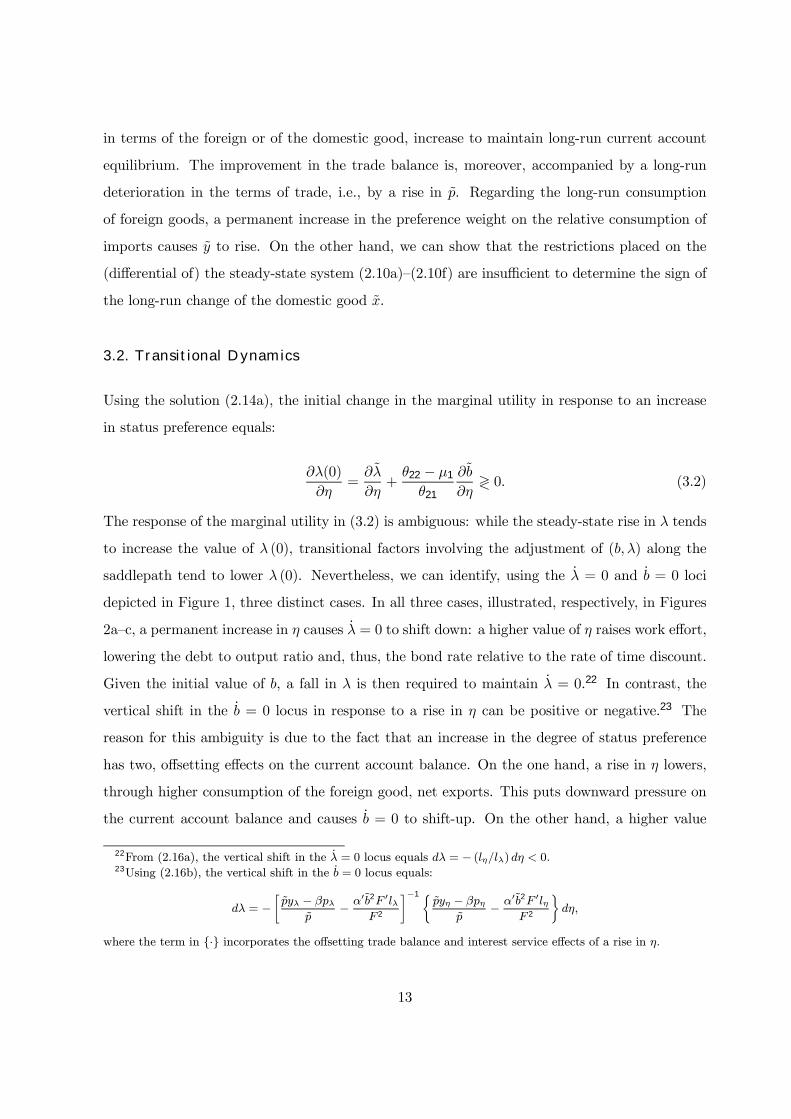
in terms of the foreign or of the domestic good, increase to maintain long-run current account

equilibrium. The improvement in the trade balance is, moreover, accompanied by a long-run

deterioration in the terms of trade, i.e., by a rise in p. Regarding the long-run consumption

of foreign goods, a permanent increase in the preference weight on the relative consumption of

imports causes y to rise. On the other hand, we can show that the restrictions placed on the

(differential of) the steady-state system (2.10a)(2.10f) are insufficient to determine the sign of

the long-run change of the domestic good x.

3.2. Transitional Dynamics

Using the solution (2.14a), the initial change in the marginal utility in response to an increase

in status preference equals:

∂λ(0)

∂η=∂λ

∂η+θ22 − µ1

θ21

∂b

∂η≷ 0. (3.2)

The response of the marginal utility in (3.2) is ambiguous: while the steady-state rise in λ tends

to increase the value of λ (0), transitional factors involving the adjustment of (b,λ) along the

saddlepath tend to lower λ (0). Nevertheless, we can identify, using the úλ = 0 and úb = 0 loci

depicted in Figure 1, three distinct cases. In all three cases, illustrated, respectively, in Figures

2ac, a permanent increase in η causes úλ = 0 to shift down: a higher value of η raises work effort,

lowering the debt to output ratio and, thus, the bond rate relative to the rate of time discount.

Given the initial value of b, a fall in λ is then required to maintain úλ = 0.22 In contrast, the

vertical shift in the úb = 0 locus in response to a rise in η can be positive or negative.23 The

reason for this ambiguity is due to the fact that an increase in the degree of status preference

has two, offsetting effects on the current account balance. On the one hand, a rise in η lowers,

through higher consumption of the foreign good, net exports. This puts downward pressure on

the current account balance and causes úb = 0 to shift-up. On the other hand, a higher value

22From (2.16a), the vertical shift in the úλ = 0 locus equals dλ = − (lη/lλ) dη < 0.23Using (2.16b), the vertical shift in the úb = 0 locus equals:

dλ = −·pyλ − βpλ

p− α0b2F 0lλ

F 2

¸−1½pyη − βpη

p− α0b2F 0lη

F 2

¾dη,

where the term in · incorporates the offsetting trade balance and interest service effects of a rise in η.

13

of η encourages greater work effort (and output), which, given b0, lowers the bond rate rb and

interest service. The latter effect tends to improve the current account balance, which, in turn,

leads úb = 0 to shift down.24

Figures 2a and 2b illustrate the case in which the trade balance effect dominates so that the

úb = 0 locus shifts up in response to a permanent increase in the status preference parameter

η. The distinction between the two phase diagrams is that in Figure 2a, the vertical decline in

the úλ = 0 locus exceeds that of the úb = 0 locus in absolute value, while the opposite is true

in Figure 2b. In Figure 2a this means that the new saddlepath, described by the line DE, lies

below its original position (not depicted), implying that λ (0) falls from point A to point D before

proceeding up DE. In contrast, the new saddlepath GH in Figure 2b lies above its initial position

so that λ (0) rises from point A to point G at t = 0. The cases illustrated by Figures 2a and

2b are further distinguished by the initial responses of domestic and foreign goods consumption

and the terms of trade: combined with the direct effect of a higher value of η [see (2.8a)(2.8c)],

the fall in λ (0) in Figure 2aand also below in Figure 2cresults in a rise in x(0) and y(0)

and a fall in p(0). In contrast, the initial response of these variables is ambiguous in the case of

Figure 2b in which λ (0) rises. Nevertheless, the transitional adjustment to long-run equilibrium

in both Figures 2a and 2b along the saddlepaths DE and GH involves, as established in (2.15),

increasing values of the marginal utility and the stock of debt, i.e., úλ > 0, úb > 0 and, thus,

reductions in the levels of domestic and foreign consumption, úx < 0, úy < 0, and a depreciation

in the terms of trade, úp > 0. Figure 2c illustrates the case in which the úb = 0 locus shifts down

in response to a rise in η: in other words, the interest service effect described above dominates

the trade balance effect. Here, the jump in λ (0) from point A to point J is unambiguously

negative. Nevertheless, as in Figures 2a and 2b, the marginal utility and the stock of debt rise

toward their steady-state values, in this case along the new saddlepath JL.25

To further describe the response of the economy to a shift in status preference, we conclude

this section of the paper by considering the behavior of the trade balance, the bond rate rb,

24If rb is solely a function of b, then úλ = 0 does not shift in response to an increase in η. Moreover, since úb = 0unambiguously shifts up in this case, the shadow value immediately rises to λ with no transitional dynamics.Note, however, that for macroeconomic disturbances such as world interest rate shocks, the speciÞcation of rb asa function of b alone suffices to generate an interior equilibrium with saddlepoint dynamics.

25The shift in úλ = 0 in Figure 2c must, however, sufficiently exceed that of úb = 0 in order for the long-runequilibrium at point L to correspond to higher values of λ and b.

14

and the domestic rate of return rd.26 Linearizing the expression for the trade balance about the

steady-state equilibrium (2.10a)(2.10f) and substituting for (2.14a)(2.14b), its solution path

corresponds to:

TB = ρb− (pyλ − βpλ)(θ22 − µ1)

pθ21(b− b0)eµ1t. (3.3)

Differentiating (3.3) with respect to η and evaluating at t = 0, the initial response of the trade

balance equals:∂TB(0)

∂η=

·ρ− (pyλ − βpλ)(θ22 − µ1)

pθ21

¸∂b

∂η. (3.4a)

Using the deÞnition of θ21 and substituting for θ22 in (3.4a), we can demonstrate that the change

in the trade balance at t = 0 is given by:

∂TB(0)

∂η= θ−1

21 [µ1p−1(pyλ − βpλ)− (b/λ) det (J)] < 0. (3.4b)

Thus, a permanent increase in η causes the trade balance to deteriorate on impact, a result

true for all three cases described abovethat depends on the sufficient condition that the long-

run equilibrium is a saddlepoint, i.e., det (J) < 0. Using the solution path (3.3), it is clear,

nevertheless, that subsequent to t = 0 the trade balance improves continuously in order to

support the rising stock of debt. Regarding the interest rates rb and rd, we show in the appendix

that their solution paths correspond, respectively, to:

rb = ρ+α0µ1

F (θ11 − µ1)(b− b0)eµ1t, (3.5a)

rd = ρ+α0µ1

F (θ11 − µ1)(1− pλλ/p)(b− b0)eµ1t. (3.5b)

Evaluating (3.5a, b) at t = 0 and combining, we show that both rates initially fall in response

to a permanent increase in η, i.e.:

∂rd(0)

∂η= (1− pλλ/p)∂r

b(0)

∂η< 0. (3.6)

The expression reveals two crucial aspects of the economys short-run adjustment. One is the

26The procedure used to obtain the solutions of these variables is found, in the appendix, equations (6.4a)(6.4b), (6.5a)(6.5c), and (6.6a)(6.6b), respectively.

15

fact that since rb declines on impact, it must case that the debt to GDP ratio falls at t = 0. Since

the stock of debt is given at t = 0, this means that employment and output initially increase in

response to the rise in η, a result that obtains whether or not λ(0) rises or falls. As a consequence,

interest service declines in the short-run, which implies that the initial current account deÞcits

are caused by the short-run deterioration (eventually reversed) in the trade balance. The other

aspect is that the domestic rate of return rd, while also below its long-run value of ρ, lies above

the bond rate at t = 0. This is due to the fact that terms of trade depreciates at t = 0, i.e.,

úp/p = pλ úλ(0)/p > 0, which, under interest rate parity, raises the domestic rate relative to the

bond rate.27 Finally, both interest rates rise for t > 0, converging to their common steady-

state value of ρ, reßecting both accumulation of debt, which increases the bond rate, and the

continued appreciation in the terms of trade, which raises the internal rate. The adjustment

paths of the two rates are illustrated in Figure 3, which depicts the initial declines in rb(0) and

rd(0) and their subsequent convergence to ρ.

4. The Planner’s Problem and Optimal Taxation

4.1. Intertemporal Equilibrium

In this section of the paper we derive the solution to the model from a social planners point

of view. The key distinction between the solution of the planners problem and that of the

representative agent is that the planner internalizes the consumption and borrowing external-

ities ignored by the representative agent. In terms of the consumption externality, the planner

assigns to each identical agent the same level of imported goods, y = Y . Likewise, the planner

sets the level of work effort and the stock of debt to take into account the fact that these choices

affect the interest rate rb at which the economy borrows from abroad. To distinguish the Pareto

optimal solution from its decentralized counterpart, we denote the variables of the optimal so-

lution with the superscript o.28 The social planners optimization problem is thus formulated

in the following way

max

Z ∞

0[U(xo, yo) + δs (1) + V (lo)]e−ρtdt, (4.1a)

27We can show that the term (1− pλλ/p) in (3.5b), while less than unity, is positive.28It is assumed in this section that functions are evaluated at their Pareto optimal values, e.g., F = F (lo).

16

subject to

úbo = yo + [xo − F (lo)]/po + r∗ + α[bo/F (lo)]bo, bo(0) = bo0 > 0, (4.1b)

where, as before, ρ is the exogenous rate of time preference and po is the relative price of the

foreign in terms of the domestic good. We substitute expression for the bond rate rb[bo/F (lo)]

in (4.1b) to emphasize the fact the planner takes into account the effect that work effort and

borrowing decisions have on the bond rate. Solving this problem, the following socially optimal

equilibrium is derived

Ux (xo, yo) = λo/po, Uy (x

o, yo) = λo, (4.2a, b)

V 0(lo) +λoα0(bo)2F 0

F 2(lo)= −λoF 0(lo)/po, F (lo) = xo + Z(po), (4.2c, d)

úλo = λoρ− rb[bo/F (lo)]− α0bo/F (lo), úbo = yo − Z(po)/po + rb[bo/F (lo)]bo, (4.2e, f)

where λo is the current Pareto optimal costate variable and where the market clearing condition

(4.2d) and current account relationship (4.2f) are added to complete the system. Examining

the optimality conditions in equations (4.2a)(4.2f), we see the crucial differences between the

Pareto and decentralized economies. In (4.2b), there is no externality from the consumption

of imports. Indeed, because the planner sets y = Y prior to the calculating the optimality

conditions, status considerations and, in particular, the parameter η, play no role in the social

optimum. In (4.2c) the planner incorporates into his evaluation of the disutility of work effort the

fact that a greater level of employment lowers the interest cost of borrowing. Similarly, in (4.2e)

the planner takes into account that additional indebtedness raises the interest cost of borrowing.

In addition, the equilibrium (4.2a)(4.2f) implicitly incorporates, as in the decentralized case,

a transversality condition limt→∞ λoboe−ρt = 0 guaranteeing that the necessary conditions are

sufficient for an optimum.

An important implication of the optimality condition (4.2c) for work effort is that the in-

stantaneous solutions in the planners equilibrium depend, in addition to the marginal utility λo,

on the stock of debt bo. In other words, equations (4.2a)(4.2d) constitute a short-run system

that is solved for as follows

xo = x(λo, bo), xoλ < 0, xob > 0; yo = y(λo, bo), yoλ < 0, yob > 0, (4.3a, b)

17

po = p(λo, bo), poλ > 0 pob > 0; lo = l(λo, bo), loλ > 0, lob > 0, (4.3c, d)

where the signs of the partial derivatives of (xo, yo, po, lo) with respect to the marginal utility of

wealth λo and the stock of debt bo are indicated in (4.3a)(4.3d).29 The partial derivatives with

respect to λo have an interpretation similar to that the decentralized model. In contrast, the

partial derivatives with respect to debt bo in the social equilibrium are explained as follows: a

higher stock of debt lowers the disutility of labor, since greater work effort implies that a larger

stock of debt is less costly in terms of debt service. As such, employment rises, lob > 0, which

results in an expansion in domestic output that causes a fall in the terms of trade, pob > 0. The

latter implies, in turn, an increase in domestic consumption, xob > 0, and, because Uxy > 0, a

rise in foreign consumption, yob > 0.

Substituting the instantaneous solutions (4.3b)(4.3d) into (4.2e, f), we obtain the differential

equation system that describes the evolution of the marginal utility of wealth and stock of debt

úλo = λo½ρ−

·r∗ + α

µbo

F [l(λo, bo)]

¶¸− bo

F [l(λo, bo)]α0µ

bo

F [l(λo, bo)]

¶¾, (4.4a)

úbo = y (λo, bo)− Z [p (λo, bo)]

p (λo, bo)+

½r∗ + α

·bo

F [l(λo, bo)]

¸¾bo, (4.4b)

where we substitute in (4.4a, b) for the bond rate. Setting úλo = úbo = 0 in (4.4a, b), the

steady-state equilibrium of the social planner corresponds to

Ux(xo, yo) = λo/po, Uy (x

o, yo) = λo, (4.5a, b)

V 0(lo) +λoα0(bo)2F 0

F 2(lo)= −λoF 0(lo)/po, F (lo) = xo + Z(po), (4.5c, d)

rb[bo/F (lo)] + α0bo/F (lo) = r∗ + α[bo/F (lo)] + α0bo/F (lo) = ρ, (4.5e)

Z (po)− poyo = por∗ + α[bo/F (lo)]bo, (4.5f)

where, as before, the symbol indicates a long-run variable. Similar to the decentralized frame-

work, equations (4.5a)(4.5d) are the long-run counterparts to (4.2a)(4.2d), while (4.5e) and

(4.5f) are, respectively, the steady-state Euler and current account relationships in the social

29The expressions for the partial derivatives of the socially optimal economy are stated in the appendix, equa-tions (6.7a)(6.7d) and (6.8a)(6.8d).

18

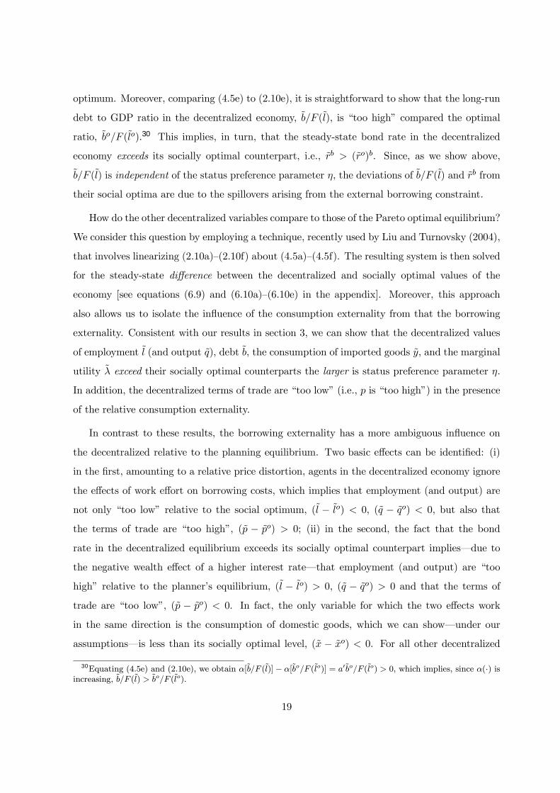
optimum. Moreover, comparing (4.5e) to (2.10e), it is straightforward to show that the long-run

debt to GDP ratio in the decentralized economy, b/F (l), is too high compared the optimal

ratio, bo/F (lo).30 This implies, in turn, that the steady-state bond rate in the decentralized

economy exceeds its socially optimal counterpart, i.e., rb > (ro)b. Since, as we show above,

b/F (l) is independent of the status preference parameter η, the deviations of b/F (l) and rb from

their social optima are due to the spillovers arising from the external borrowing constraint.

How do the other decentralized variables compare to those of the Pareto optimal equilibrium?

We consider this question by employing a technique, recently used by Liu and Turnovsky (2004),

that involves linearizing (2.10a)(2.10f) about (4.5a)(4.5f). The resulting system is then solved

for the steady-state difference between the decentralized and socially optimal values of the

economy [see equations (6.9) and (6.10a)(6.10e) in the appendix]. Moreover, this approach

also allows us to isolate the inßuence of the consumption externality from that the borrowing

externality. Consistent with our results in section 3, we can show that the decentralized values

of employment l (and output q), debt b, the consumption of imported goods y, and the marginal

utility λ exceed their socially optimal counterparts the larger is status preference parameter η.

In addition, the decentralized terms of trade are too low (i.e., p is too high) in the presence

of the relative consumption externality.

In contrast to these results, the borrowing externality has a more ambiguous inßuence on

the decentralized relative to the planning equilibrium. Two basic effects can be identiÞed: (i)

in the Þrst, amounting to a relative price distortion, agents in the decentralized economy ignore

the effects of work effort on borrowing costs, which implies that employment (and output) are

not only too low relative to the social optimum, (l − lo) < 0, (q − qo) < 0, but also that

the terms of trade are too high, (p − po) > 0; (ii) in the second, the fact that the bond

rate in the decentralized equilibrium exceeds its socially optimal counterpart impliesdue to

the negative wealth effect of a higher interest ratethat employment (and output) are too

high relative to the planners equilibrium, (l − lo) > 0, (q − qo) > 0 and that the terms of

trade are too low, (p − po) < 0. In fact, the only variable for which the two effects work

in the same direction is the consumption of domestic goods, which we can showunder our

assumptionsis less than its socially optimal level, (x − xo) < 0. For all other decentralized

30Equating (4.5e) and (2.10e), we obtain α[b/F (l)]− α[bo/F (lo)] = a0bo/F (lo) > 0, which implies, since α(·) isincreasing, b/F (l) > bo/F (lo).

19

variables, including the consumption of foreign goods, the stock of debt, and the marginal

utilityit is ambiguous whether they are higher or lower than their corresponding values in the

socially optimal economy.31

Taking Þrst-order approximations of (4.4a, b) around the steady state (45a)(4.5f), the

following matrix differential equation is obtained

úλo

úbo

=

θo11 θo12

θo21 θo22

λo − λo

bo − bo

, (4.6a)

where

θo11 =λoF 0loλb

o

F 2[2α0 + α00bo/F ] > 0, θo12 = −

λo(F − F 0lobbo)F 2

[2α0 + α00bo/F ],

θo21 =

"poyoλ − βopoλ

po− α

0(bo)2F 0loλF 2

#< 0, θo22 =

"ρ+

α0bo[F − F 0lobbo]F 2

+poyob − βopob

po

#,

(4.6b)

and where βo = Z0 − Z(po)/po is substituted into the element θo21. The signs of the trace and

determinant of the Jacobian matrix Jo of (4.6a) determine the local dynamics of the social

optimum. These relationships correspond to

tr(Jo) = µo1 + µo2 = θ

o11 + θ

o22

= ρ+λoF 0loλb

o

F 2(2α0 + α00bo/F ) +

α0bo(F − F 0lobbo)F 2

+poyob − βopob

po, (4.7a)

det(Jo) = µo1µo2 = θ

o11θ

o22 − θo12θ

o21

=λo

F 2(2α0 + α00bo/F )

½(F − F 0lobbo)

poyoλ − βopoλpo

+ F 0loλbo

·ρ+

poyob − βopobpo

¸¾, (4.7b)

where µo1, µo2 are the eigenvalues of Jo such the following characteristic equation is satisÞed:

(µo)2 − [tr(Jo)]µo + det (Jo) = 0. For planners economy to possess a saddlepoint equilibrium,det(Jo) = µo1µ

o2 < 0. This obtains if the term in · brackets in (4.7b) is negative, i.e.:

det(Jo) = µo1µo2 < 0 ⇔ (F − F 0lobbo)

poyoλ − βopoλpo

+ F 0loλbo

·ρ+

poyob − βopobpo

¸< 0.

31We can show, nevertheless, that the wealth effect lowers y relative to yo and raises λ relative to λo.

20

If this condition is satisÞed, then the equilibrium of the planners problem, like its decentralized

counterpart, is a saddlepoint, with Jo possessing a negative and a positive eigenvalue: µo1 < 0,

µo2 > 0, | µo1 |< µo2.32 As in the decentralized framework, we can solve for the following stable

saddlepath that describes the transitional adjustment of (b,λ):

(λo − λo) = −θo22 − µo1θo21

(bo − bo) = −θo12

θo11 − µo1(bo − bo) = θo12

θo11 − µo1(bo − bo0)eµ

o1t. (4.8)

Using equations (4.4a, b), the úλo = 0 and úbo = 0 loci in the socially optimal framework are

described by the following relationships:

r∗ + α·

bo

F [l(λo, bo)]

¸+

bo

F [l(λo, bo)]α0·

bo

F [l(λo, bo)]

¸= ρ, (4.9a)

Z[p(λo, bo)]

p(λo, bo)− y(λo, bo) =

½r∗ + α

·bo

F [l(λo, bo)]

¸¾bo. (4.9b)

In contrast to the decentralized model, however, the úλo = 0 and úbo = 0 loci in the planning

framework are not unambiguously positive relationships. This is evident from the expressions

for their slopes, which correspond, respectively, to

(dλ/db)o |λ=0 = (F − F 0lobbo)/boF 0loλ, (dλ/db)o |b=0 = −θo22/θo21,

where the term (F − F 0lobbo) in the expression for (dλ/db)o |λo=0 is ambiguous in sign, as is the

element θo22 in (dλ/db)o |bo=0.

33 Given the ambiguity of the slopes of the úλo = 0 and úbo = 0 loci,

there are six possible (local) cases, yielding six distinct (local) equilibria. Here, we brießy focus

on the three cases that yield saddlepoints (the equilibria in the other three cases correspond to

unstable nodes). The Þrst case we considerillustrated in Figure 4ais the one in which the

úλo = 0 locus is positively sloped, while the úbo = 0 locus, unlike in the decentralized framework,

is negatively sloped:

(dλ/db)o |λo=0 > 0 > (dλ/db)o |bo=0.

32In contrast to the decentralized model, the stability properties of the planners equilibrium depend, throughthe partial derivatives (yob , p

ob , l

ob) directly on the slope and curvature properties of α(·).

33The term (F − F 0lobbo) in (dλ/db)o |λo=0 can be rewritten as (F − F 0lobbo) = (1 − ωoqlωolb)F , where ωoql =(∂F/∂l)(l/F ) and ωolb = (∂l/∂b)(b/l) are, respectively, the elasticities of output with respect to employment andemployment with respect to debt. Thus, if ωoqlω

olb exceeds unity, then úλ

o = 0 is negatively sloped.

21

What is the intuition behind a negatively-sloped úbo = 0 locus? Recall that in the social optimum

[see (4.3d)] an increase in bo encourages work effort. This lowers, in turn, the debt to GDP

ratio and the bond rate, which tends to improve the current account (úbo < 0). Moreover, in this

context, a higher level of bo has relative price and trade balance effects that also lead to úbo < 0. If

together these effects are sufficiently strong, they then dominate the direct negative implications

for the current account balance that a higher value of bo has on interest service, thus requiring

a fall in λo to maintain úbo = 0, as is depicted in Figure 4a. As in the decentralized framework,

saddlepathVV leading (bo,λo) to the equilibriumQ in Figure 4a is positive relationship, although

its slope, in general, differs from SS in Figure 1.

The second casedepicted in Figure 4billustrates the situation in which both the úλo = 0

and úbo = 0 loci are negatively sloped, with úλo = 0 steeper in absolute value:

(dλ/db)o |λo=0 < (dλ/db)o |bo=0 < 0.

How do we account for a negatively sloped úλo = 0 locus, which is the case as long as (F −F 0lobb

o) < 0? As indicated, a rise in bo leads to greater employment and, thus, to a fall in

rb[bo/F (lo)]. From the Euler equation (4.2e), this leads to úλo > 0 unless the level of λo also

declines, the latter causing a rise in leisure that keeps úλo = 0. An important implication of

this case is thatin contrast to our previous examplesthe stable saddlepath WW is negatively

sloped, implying that the stock of debt and its shadow value move in opposite directions in the

transition to steady-state equilibrium, i.e., sgn (úbo) = −sgn ( úλo). What are the implications

of the negatively sloped WW locus? Consider the situation in which the initial stock of debt,

as in the decentralized economy in Figure 1, is less than its long-run value, bo0 <bo. The

planner then chooses a declining path along WW starting at point R, with úλo < 0, úbo > 0.

From (4.3a, b), it is clear that adjustment toward point Q involves risinginstead of falling

domestic and foreign consumption: úxo = xoλúλo + xob

úbo > 0, úyo = yoλúλo + yob

úbo > 0. Nevertheless,

to close the current account deÞcit (úb > 0) between points R and Q, we can show that there

must be a corresponding surplus on the trade balance, reßecting in the social optimum the

direct positive effects of growing levels of debt on the relative price and output.34 Finally,

the third saddlepoint case in the planners economy is qualitatively identical to that of the

34The solution path of the trade balance in the social optimum is derived in appendix, equations (6.11a)(6.11b)

22

decentralized economy, i.e., both úλo = 0 and úbo = 0 are positively sloped, with úλo = 0 steeper

than úbo = 0: (dλ/db)o|λo=0 > (dλ/db)o |bo=0 > 0. The corresponding phase diagram in this

instance is qualitatively the same as Figure 1 and is not reproduced here.

4.2. Optimal Policy

In this section of the paper, we derive the optimal policy to offset the relative consumption, work

effort, and borrowing externalities characterizing the decentralized economy. Given the fact that

there are three distinct externalities, three separate policy tools are required to attain the social

optimum. We assume that the policy tools available to public sector include a tariff on levied

on the imported good, τy, a tax on domestic labor, τl, (amounting to a tax on output in this

single-factor framework), and surcharges, or penalties, τb, on international interest service.

The decentralized individual budget constraint (2.4b) then becomes

úb = (1 + τy)y +x− (1− τl)F (l)

p+ (1 + τb) r

b[b/F (l)]b+ T, (4.10)

where the government budget is closed by a continuous adjustment in lump-sum transfers (or

taxes), T : τyy + τlF (l) /p + τbrb[b/F (l)]b = T . Solving the decentralized problem of section 2

under these constraints, it is straightforward to show that the necessary optimality conditions

in the symmetric equilibrium become:35

Ux(x, y) = λ/p, Uy (x, y) + ηy−1 = (1 + τy)λ, (4.11a, b)

V 0(l) = −λ (1− τl)F0(l)

p, úλ = λρ− (1 + τb) rb[b/F (l)]. (4.11c, d)

The decentralized economy reproduces the planners optimum if the solutions for decentralized

case coincide with their Pareto optimal counterparts, i.e.: x = xo, y = yo, λ = λo, l = lo, p = po,

and b = bo. The latter obtains if the decentralized optimality conditions for imports, work effort,

and borrowing, represented by (4.11b)(4.11d), equal their socially optimal counterparts (4.2b,

35In all other respects, the properties of the decentralized framework remain the same as in section 2. In additionto imposing a transversality condition insuring sufficiency, we assume that the introduction of distortionarytaxation does not affect the saddlepoint property of the decentralized equilibrium, i.e., a condition analogous to(2.13) obtains in this context.

23

c, e):

Uy (x, y) + ηy−1 = (1 + τy)Uy (x, y) , (4.12a)

V 0(l) +(1− τl)λF 0(l)

p= V 0(l) +

λα0b2F 0

F 2(l)+λF 0(l)p

, (4.12b)

(1 + τb) [r∗ + α[b/F (l)]] = r∗ + α[b/F (l)] + α0b/F (l). (4.12c)

Solving (4.12a)(4.12c) in terms of the relevant policy instrument, we obtain following optimal

tariff, output tax, and interest surcharge (τ∗y , τ∗l , τ∗b ):

τ∗y =η

Uy (x, y) y> 0, τ∗l = −

pα0b2

F 2(l)< 0, τ∗b =

α0bF (l)rb[b/F (l)]

> 0.

Thus, the optimal policy to offset the effects of relative consumption and borrowing externalities

is to levy a positive tariff on imports, a subsidyrather than a taxon employment (output),

and a positive charge, or penalty, on international interest payments. In other words, the

over-consumption of imported goods should be deterred by an appropriate tariff, work effort

should be subsidized to achieve the optimal debt to GDP ratio given the upward-sloping interest

rate relationship, and, similarly, international borrowing should be penalized to internalize the

interest cost externality of greater indebtedness.36

5. Conclusions

This paper employs a standard developing economy framework to consider the interactions of

macroeconomic spillovers. The particular externalities we consider are consumption externali-

ties and spillovers arising from an external borrowing constraint. The consumption externality

reßects the assumption that agents social status depends on their relative consumption of im-

ported goods, while the upward-sloping interest rate relationship leads agents to neglect the

effects of their borrowing decisions on the interest cost of their international obligations. A key

feature of the external borrowing constraint is that interest costs are a positive function of the

debt to GDP ratio. This speciÞcation has important implications for the economys saddlepoint

36Observe, for example, that τ∗y rises with the degree of status preference η and that τ∗l increases (in absolute

value) the lower is the terms of trade p. Finally, note that τ∗b coincides with the partial elasticity of the bond raterb with respect to the stock of debt b.

24

dynamics and results in a production externality as well as a direct borrowing externality.

The goal of this paper is to analyze an economy characterized by these phenomena and contrast

its behavior with that of the social planners.

To brießy highlight some of the chief results of the paper, we analyzed the response of the

open economy in the decentralized equilibrium to a permanent rise in the preference weight

that agents place on status considerations. We show that this leads to a long-run rise in employ-

ment and outputconsistent with closed economy studies of this issueand to current account

deÞcits, declines in the consumption of domestic and foreign goods, and a depreciation in the

terms of trade during the transition to the steady-state equilibrium. We also Þnd that the bond

rate and the domestic interest rate decline on impact and then increase toward their common

steady-state value, the exogenous time rate of preference. Due to the depreciation in the terms

of trade, the domestic rate lies above the bond rate during the transition.

In the second half of the paper, we study the contrasting steady-state and dynamic properties

of the social planners equilibrium. Focusing on the implications of the borrowing externality,

we show that the steady-state debt to GDP ratio and bond rate are too high and the long-run

consumption of domestic goods is too low in the decentralized equilibrium relative to the social

optimum. Regarding the other variables, it is ambiguous whether their long-run values are higher

or lower than their socially optimal counterparts, due to the offsetting effects of the resulting

relative price and wealth distortions. We also derive the intertemporal properties of the planners

economy and show that saddlepath for debt and the marginal utility of wealth can be negatively

sloped, which is in contrast to the upward-sloping saddlepath in the decentralized case. Finally,

we demonstrate that the optimal policy combination to achieve the Pareto optimum involves a

tariff on imports, a subsidy on employment, and a penalty on international borrowing.

6. Appendix

6.1. Partial Derivatives in (2.8a)—(2.8d)

Differentiating the instantaneous decentralized equilibrium (2.6a)(2.6d) with respect to λ, we

calculate the following partial derivatives.

25

(i) For λ:

xλ = −D−1©£¡Uyy − ηy−2

¢/p− Uxy

¤ΛZ 0 + Uxyλ(F 0)2/p2

ª< 0, (6.1a)

yλ = −D−1©£(Uxx − Uxy/p)Z0 − λ/p2

¤Λ−Uxxλ(F 0)2/p2

ª< 0, (6.1b)

pλ = D−1£Uxx(Uyy − ηy−2)− U2

xy

¤ ¡F 0¢2/p+

£(Uyy − ηy−2)/p− Uxy

¤Λ > 0, (6.1c)

lλ =¡F 0/pD

¢ ©£Uxx

¡Uyy − ηy−2

¢− U2xy

¤Z0 −Uxyλ/p

ª> 0. (6.1d)

(ii) For η:

xη = Uxy/yD©λ(F 0)2/p2 −ΛZ0ª > 0, (6.2a)

yη = −(yD)−1©Uxx

£λ(F 0)2/p2 − ΛZ0¤+ Λλ/p2

ª> 0, (6.2b)

pη = (yD)−1UxyΛ < 0, lη = UxyλF

0/p2yD > 0, (6.2c, d)

where D = [Uxx(Uyy − ηy−2) − U2xy][λ (F

0)2 /p2 − ΛZ 0] + (Uyy − ηy−2)Λλ/p2 > 0 and Λ =

(V 00 + λF 00/p) < 0. To guarantee that leisure is a normal good, we impose [Uxx(Uyy − ηy−2)−U2xy]Z

0 − Uxyλ/p > 0 in (6.1d).

6.2. Expressions for the Long-Run Comparative Statics

Differentiating the steady-system (2.10a)(2.10f) with respect to η, we derive the following long-

run comparative statics expressions discussed in section 3.

∂b

∂η=−α0b(F 0)2yF 2∆

[βUxy/p− Z0Uxx] > 0, (6.3a)

∂l

∂η=¡F 0¢−1 ∂q

∂η=−α0F 0yF∆

[βUxy/p−Z 0Uxx] > 0, (6.3b)

∂λ

∂η=−α0yF∆

nUxxp[Z

0Λ− λ ¡F 0¢2/p2]− Λ(Uxyβ + λ/p) + ρUxyλb

¡F 0¢2/(F p)

o> 0, (6.3c)

∂p

∂η=−α0yF∆

[(F 0)2(ρUxyb/F − Uxx)− Λ] > 0, (6.3d)

∂x

∂η=−α0yF∆

[−Uxy¡F 0¢2(ρbZ0/F − β/p) + Z 0Λ] ≷ 0, (6.3e)

∂y

∂η=−α0yF∆

[Uxx(F0)2(ρbZ0/F − β/p)− βΛ/p] > 0, (6.3f)

26

where

∆ =α0

F

nUxxλ

¡F 0¢2/p+ Λ[λ/p− Z0(Uxxp−Uxy)] + βΛ[Uxy − 1/p(Uyy − ηy−2)]

o−α0(F 0)2/F [ρbUxyλ/pF − Γ(ρbZ0/F − β/p)] < 0,

letting Λ = (V 00 + λF 00/p) < 0 and Γ = [Uxx(Uyy − ηy−2) − U2xy] > 0. To insure ∆ < 0, we

impose the sufficient condition (ρbZ 0/F − β/p) < 0, which also guarantees ∂y/∂η > 0 in (6.3f).

6.3. Expression for the Trade Balance

Linearizing the expression for the trade balance in terms of the foreign good, given by TB =

Z[p(λ, η)]/p(λ, η)− y(λ, η), we obtain:

TB = Z(p)/p− y − p−1(pyλ − βpλ)(λ− λ). (6.4a)

Substituting for (2.14a) and using the fact that Z(p)/p− y = ρb, we derive the solution path forthe trade balance:

TB = ρb− (pyλ − βpλ)(θ22 − µ1)

pθ21(b− b0)eµ1t. (6.4b)

6.4. Expressions for rb and rd

(i) For rb:

Linearizing (2.3) and substituting the expressions (2.14a)(2.14b), we obtain the following

solution path for the bond rate rb:

rb = ρ− α0

Fθ21[θ21 +bF

−1F 0lλ (θ22 − µ1)](b− b0)eµ1t. (6.5a)

To simplify (6.5a), we substitute for (θ22 − µ1) = θ12θ21/ (θ11 − µ1), using the characteristic

equation (2.12c):

rb = ρ− α0

F (θ11 − µ1)[(θ11 − µ1) + bF

−1F 0lλθ12](b− b0)eµ1t. (6.5b)

27

This expression can be further reduced by substituting into (6.5b) the elements θ11, θ12 from

the Jacobian matrix J of (2.11a). This yields

rb = ρ+α0µ1

F (θ11 − µ1)(b− b0)eµ1t, (6.5c)

and is the basis of our discussion regarding the adjustment of rb in section 2.

(ii) For rd:

From the deÞnition (2.7), substituting for (6.5c) and for úλ using (2.14a), the expression for

the domestic rate of return rd corresponds to:

rd = rb + pλ úλ/p = ρ+ µ1

·α0

F (θ11 − µ1)+pλ (θ22 − µ1)

pθ21

¸(b− b0)eµ1t. (6.6a)

Using the fact that (θ22 − µ1)/θ21 = θ12/(θ11 − µ1) and substituting for θ12, we can show that

(6.6a) simpliÞes to:

rd = ρ+α0µ1(1− pλλ/p)F (θ11 − µ1)

(b− b0)eµ1t. (6.6b)

We can show that the (1− pλλ/p) term in (6.6b) equals −(V 00+λF 00/p)lλ/F 0, which positive aslong as leisure is a normal good, i.e., lλ > 0.

6.5. Partial Derivatives of (4.3a)—(4.3d)

Differentiating the instantaneous Pareto-optimal equilibrium (4.2a)(4.2d) with respect to λo

and bo, we calculate the following partial derivatives.

(i) For λo:

xoλ = −(Do)−1(Uyy/p− Uxy)(Λo + γ)Z0 + λF 0/(po)2(UxyF 0 + Uyy²) < 0, (6.7a)

yoλ = −(Do)−1[(Uxx−Uxy/po)Z0−λo/(po)2](Λo+ γ)−λoF 0/(po)2(UxxF 0−Uxy²) < 0, (6.7b)

poλ = (Do)−1(UxxUyy − U2

xy)F0 ¡F 0/po + ²¢+ (Uyy/po − Uxy)(Λo + γ) > 0, (6.7c)

loλ = (Do)−1(UxxUyy − U2

xy)Z0 ¡F 0/po + ²¢− λo/(po)2(UxyF 0 + Uyy²) > 0. (6.7d)

28

(ii) For bo:

xob = −φF 0Uyyλo/(po)2Do > 0, yob = φF0Uxyλo/(po)2Do > 0, (6.8a, b)

pob = φF0(UxxUyy−U2

xy)/Do > 0, lob = φ[(UxxUyy−U2

xy)Z0−Uyyλo/(po)2]/Do > 0, (6.8c, d)

where Do = (UxxUyy − U2xy)[λ

o (F 0)2 /(po)2 − (Λo + γ)Z0] + (Λo + γ)Uyyλo/(po)2 > 0. Note

that we have made the following substitutions into (6.7)(6.8): γ = −λo(bo)2F−4α00bo(F 0)2 −α0[F 00F 2 − 2(F 0)2] < 0, φ = λF−2F 0bo(2α0 + α00bo/F ) > 0, and ² = α0(bo)2F 0/F 2 > 0, with

Λo = (V 00 + λoF 00/po) < 0. In (6.7a) and (6.7d) we assume that sufficient conditions for xoλ < 0,

loλ > 0 obtain.

6.6. Expressions for the Deviations of Decentralized Variables from Their Social

Optima

Linearizing the decentralized steady-state (2.10a)(2.10f) about its socially optimal counterpart

(4.5a)(4.5f), we derive the following system in the deviations of (x, y, p, l, λ) from (xo, yo, po,lo, λo)

Uxx Uxy λo/(po)2 0 −(po)−1

Uxy Uyy − η(yo)−2 0 0 −10 0 −λoF 0/(po)2 V 00 + λoF 00/po F 0/po

−1 0 −Z 0 F 0 0

0 −po β poρF 0bo/F 0

x− xo

y − yo

p− pol − loλ− λo

=

0

−η/yo

λoα0(bo)2F 0/F 2

0

−Ωbo

(6.9)

where we substitute for (b−bo) = [F +F 0(l−lo)]bo/F to obtain a Þve-equation system. Clearly,(6.9) distinguishes between the effects of the relative consumption externality [embodied in

the second element of the vector on the right-hand-side of (6.9)] and the borrowing externality

29

[embodied in the third and Þfth elements of the vector on the right-hand-side of (6.9)]. They can,

thus, be considered separately. While it is straightforward to solve for the deviations in terms of

the relative consumption externality, we do not state the solutions here, since the corresponding

expressions differ from the steady-state comparative statics given in (6.3a)(6.3f) only because

the former are multiplied by the status parameter η. Solving then for the deviations in terms

of the borrowing externality, we calculate the expressions that are the basis of our discussion in

section 4

l−lo = F 0bo

∆0

(λoα0bo

F 2[λo/po − Z0(Uxxpo − Uxy) + β(Uxy − Uyy/po)] +

Ωo

po(ΓoZ 0 − Uxyλo/po)

)≷ 0,

(6.10a)

p− po = −bo∆0

(λoα0bo(F 0)2

F 2

"(poUxx − Uxy) + poρbo

F(Uyy/p

o − Uxy)#

+Ωo[Λo(Uyy/po − Uxy) + Γo(F 0)2/po

o≷ 0, (6.10b)

λ− λo =bo

∆0

(λoα0bo(F 0)2

F 2

h(Γoβ −Uxyλo/po)

i− poρbo

F[ΓoZ 0 − Uyyλo/(po)2]

−Ωo[Λo[ΓoZ0 − Uyyλo/po]− λo(F 0)2Γo/(po)2o≷ 0, (6.10c)

x− xo =bo

∆0

(λoα0bo(F 0)2

F 2

h(Uyy − poUxy)(ρboZ 0/F − β/po) + λo/(po)2

i−Ωo[Z 0Λo(Uyy/po − Uxy) + UxyλoF 0/(po)2]

o< 0, (6.10d)

y − yo = −bo∆0

(λoα0bo(F 0)2

F 2

h(Uxy/p

o − Uxx)(ρboZ0/F − β/po) + λoρbo/(F po)i

−ΩohΛo[λo/(po)2 − Z 0(Uxx − Uxy/po)] + Uxxλo(F 0)2/(po)2

io≷ 0, (6.10e)

where

∆0 = Uxxλo¡F 0¢2/po + Λo

hλo/po − Z 0(Uxxpo − Uxy) + β(Uxy − Uyy/po)

i−(F 0)2

hρboUxyλ

o/(poF )− Γo(ρboZ0/F − β/po)i< 0,

and letting Λo = (V 00+λoF 00/po) < 0, Γo = (UxxUyy−U2xy) > 0, and Ω

o = −po(ρ+α0bo/F ) < 0.To guarantee ∆0 < 0 and (x− xo) < 0, we impose the sufficient condition (ρboZ 0/F −β/po) < 0used above in (6.3a)(6.3f). Observe that we set η ≡ 0 in (6.10a)(6.10e).

30

6.7. Solution for the Trade Balance in the Social Optimum

Using (4.3b, c) the trade balance in terms of the foreign good in the social optimum is given

by TBo = Z[p(λo, bo)]/p(λo, bo)− y(λo, bo). Linearizing this expression and substituting for thesolution path (4.8), we obtain:

TBo = ρbo −½(pyoλ − βpoλ)(θo22 − µo1)

poθo21

− (pyb − βopob)θ21

po

¾(bo − bo0)eµ

o1t. (6.11a)

Using the fact that (θo22 − µo1)/θo21 = θo12/θ

o11 − µo1 and substituting for θo11 and θ

o12 from (4.6b),

we can show that (6.11a) reduces to:

TBo = ρbo+(θo11−µo1)−1detJo−(λo/F 2)(2α0+α00bo/F )F 0loλboρ−µ1(py

ob−βopob)/po(bo−bo0)eµ

o1t.

(6.11b)

Since for (local) saddlepoint equilibria detJo < 0, a sufficient condition for the term in ·brackets to be positive is [pyob−βopob]/po < 0, which holds as long as (UxxUyy−U2

xy)−Uxyλ/p2 > 0.

Differentiating (6.11a) with respect to time, it is clear that the trade balance improves along a

saddlepath in which bo0 <bo.

References

[1] Agenor, P.R., Capital Inßows, External Shocks, and the Real Exchange Rate, Journal of

International Money and Finance 17(5) (1998):71340.

[2] Bardhan, P.K., Optimum Foreign Borrowing, in Karl Shell (ed.), Essays on the Theory

of Optimal Economic Growth, Cambridge, MA: MIT Press (1967):11728.

[3] Barro, Robert J. and Xavier Sala-i-Martin, Economic Growth, New York: McGraw-Hill

(1995).

[4] Bhandari, Jagdeep, S., Nadeem Ul Haque and Stephen J. Turnovsky, Growth, External

Debt, and Sovereign Risk in a Small Open Economy, IMF Staff Papers 37(2) (1990):388

417.

[5] Chatterjee, Santanu and Stephen J. Turnovsky, Substitutability of Capital, Investment

Costs, and Foreign Aid, in S. Dowrick, R. Pitchford, and S.J. Turnovsky (eds.), Eco-

31

nomic Growth and Macroeconomic Dynamics: Recent Developments in Economic Theory,

Cambridge, UK: Cambridge University Press (2004): 138170.

[6] Cole, Harold L., George J. Mailath and Andrew Postlewaite, Social Norms, Saving Behav-

ior, and Growth, Journal of Political Economy 100(6) (1992):10921125.

[7] Corneo, Giacomo and Olivier Jeanne, On Relative Wealth Effects and the Optimality of

Growth, Economics Letters 54(1) (1997):8792.

[8] Dupor, Bill and Wen-Fang Liu, Jealousy and Equilibrium Overconsumption, American

Economic Review 93(1) (2003):42328.

[9] Easterlin, Richard, Does Economic Growth Improve the Human Lot? Some Empirical

Evidence, in P.A. David and M.W. Reder (eds.), Nations and Households in Economic

Growth: Essays in Honor of Moses Abramowitz, New York, NY: Academic Press (1974):89

125.

[10] Easterlin, Richard, Will Raising Incomes Increase the Happiness of All? Journal of

Economic Behavior and Organization 27(1) (1995):3547.

[11] Edwards, Sebastian, LDC Foreign Borrowing and the Default Risk: An Empirical Inves-

tigation, 1976-1980, American Economic Review 74(4) (1984):72634.

[12] Fisher, Walter H., An Optimizing Analysis of the Effects of World Interest Disturbances

on the Open Economy Term Structure of Interest Rates, Journal of International Money

and Finance 14(1) (1995):10526.

[13] Fisher, Walter H., Status Preference, Wealth and Dynamics in the Open Economy, Ger-

man Economic Review 5(3) (2004):335355.

[14] Fisher, Walter H. and Franz X. Hof, Relative Consumption, Economic Growth, and Tax-

ation, Journal of Economics 72(3) (2000a):24162.

[15] Fisher, Walter H. and Franz X. Hof, Relative Consumption and Endogenous Labor Sup-

ply in the Ramsey Model: Do Status-Conscious People Work Too Much?, Institute for

Advanced Studies (IHS), Economic Series #85, (2000b).

32

[16] Fisher, Walter H. and Dek Terrell, World Interest Shocks, Capital, and the Current Ac-

count, Review of International Economics 8(2) (2000):26174.

[17] Frank, Robert H., The Demand for Unobservable and Other Nonpositional Goods, Amer-

ican Economic Review 75(1) (1985):10116.

[18] Frank, Robert H., The Frame of Reference as a Public Good, Economic Journal 107(445)

(1997):18321847.

[19] Futagami, Koichi and Akihisa Shibata, Keeping One Step Ahead of the Jones: Status,

the Distribution of Wealth, and Long-Run Growth, Journal of Economic Behavior and

Organization 36(1) (1998):10926.

[20] Galõ, Jordi, Keeping Up with the Joneses: Consumption Externalities, Portfolio Choice,

and Asset Prices, Journal of Money, Credit, and Banking 26(1) (1994):16.

[21] Grossmann, Volker, Are Status Considerations Harmful for Growth?, FinanzArchiv 55(3)

(1998):35773.

[22] Liu, Wen-Fang and Stephen J. Turnovsky, Consumption Externalities, Production Ex-

ternalities, and Long-run Macroeconomic Efficiency, forthcoming, Journal of Public Eco-

nomics (2004) [available online].

[23] Oswald, Andrew J., Happiness and Economic Performance, Economic Journal 107(445)

(1997):18151831.

[24] Pitchford, John D., Optimum Borrowing and the Current Account When There Are Fluc-

tuations in Income, Journal of International Economics 26(3/4) (1989):34558.

[25] Rauscher, Michael, Conspicuous Consumption, Economic Growth, and Taxation, Journal

of Economics 66(1) (1997):3542.

[26] Turnovsky, Stephen J., International Macroeconomic Dynamics, Cambridge, MA: MIT

Press (1997).

33

A

S

S

Figure 1: Phase Diagram

λ

0b

0=λ&

0=b&

b

B

b~

)0(λ

λ~

λ

λ

b

b

0=λ&

0=b&

0=b&

0~λ

0~λ

0=′λ&

0=′λ&

A

A

)0(λ

)0(λ

1~λ

1~λ

0=′b&

0=′b&

1~b

1

~b

0=λ&

D

E

G

H

Figure 2b: Increase in Status Preference, Case 2

Figure 2a: Increase in Status Preference,Case1

0~b

0

~b

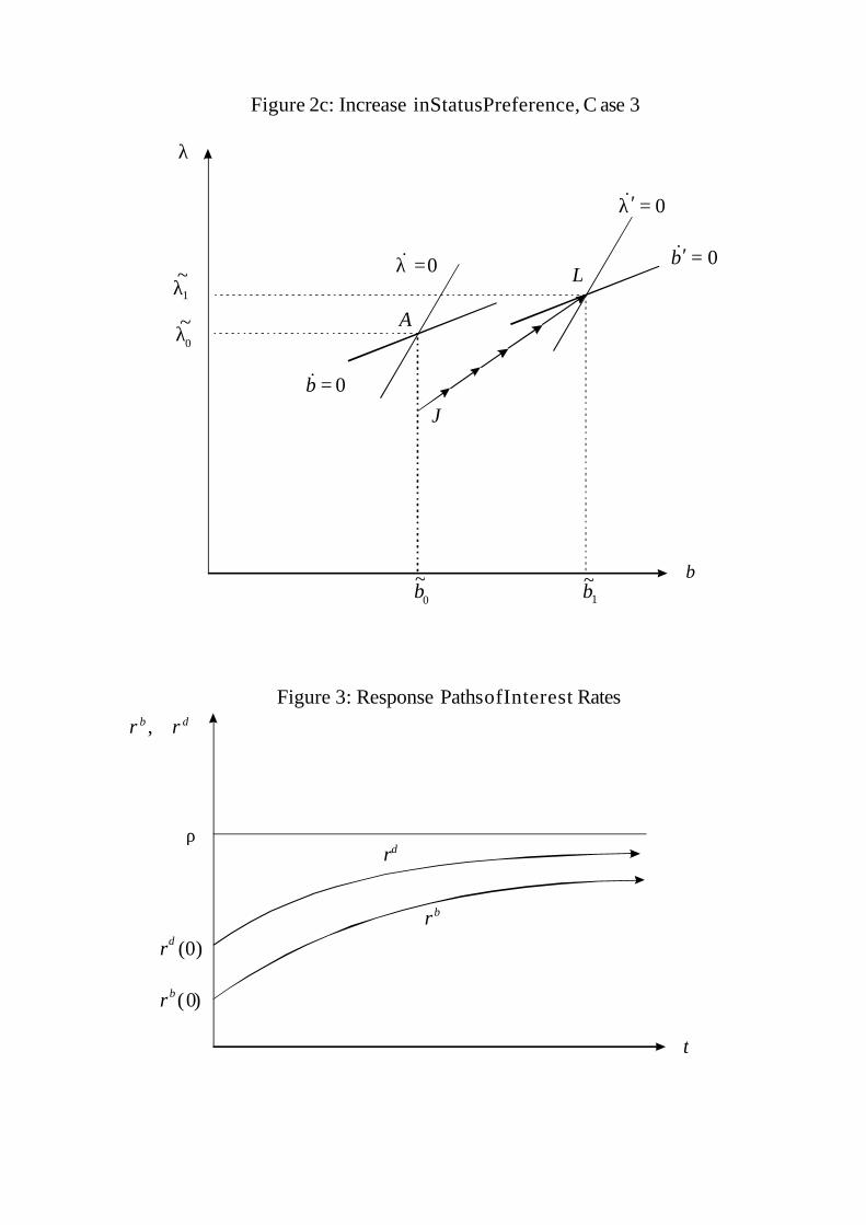
A

Figure 2c: Increase inStatusPreference, C ase 3

Figure 3: Response PathsofInterest Rates

0

~λ

λ

0=λ&

0=b&

b

0=′b&

0=′λ&

1~b

1~λ

J

L

t

ρ

db rr ,

dr

br

)0(br

)0(dr

0

~b

Figure4a:SocialEquilibrium, Case 1

Figure4b:SocialEquilibrium, Case 2

Q

Q

V

V

W

W

ob

obob

~

ob~

oλ~

oλ~

oλ

oλ

0=ob&

0=ob&

0=oλ&

ob0

0=oλ&

)0(oλ R

Author: Walter H. Fisher Title: Imports, Status Preference, and Foreign Borrowing Reihe Ökonomie / Economics Series 161 Editor: Robert M. Kunst (Econometrics) Associate Editors: Walter Fisher (Macroeconomics), Klaus Ritzberger (Microeconomics) ISSN: 1605-7996 © 2004 by the Department of Economics and Finance, Institute for Advanced Studies (IHS), Stumpergasse 56, A-1060 Vienna • +43 1 59991-0 • Fax +43 1 59991-555 • http://www.ihs.ac.at

ISSN: 1605-7996