
Implicit public debt thresholds: an empirical exercise for …€¦ · implicit public debt...
28
IMPLICIT PUBLIC DEBT THRESHOLDS: AN EMPIRICAL EXERCISE FOR THE CASE OF SPAIN Javier Andrés, Javier J. Pérez and Juan A. Rojas Documentos de Trabajo N.º 1701 2017
Transcript of Implicit public debt thresholds: an empirical exercise for …€¦ · implicit public debt...
IMPLICIT PUBLIC DEBT THRESHOLDS: AN EMPIRICAL EXERCISE FOR THE CASE OF SPAIN
Javier Andrés, Javier J. Pérez and Juan A. Rojas
Documentos de Trabajo N.º 1701
2017

IMPLICIT PUBLIC DEBT THRESHOLDS: AN EMPIRICAL EXERCISE
FOR THE CASE OF SPAIN
IMPLICIT PUBLIC DEBT THRESHOLDS: AN EMPIRICAL
EXERCISE FOR THE CASE OF SPAIN (*)
Javier Andrés
UNIVERSITY OF VALENCIA
Javier J. Pérez
BANCO DE ESPAÑA
Juan A. Rojas
ESM
(*) The views expressed in this paper are the authors’ and do not necessarily reflect those of the Banco de España, the Eurosystem or the ESM. We wish to express our thanks for the helpful comments of participants – in particular Alexander Mahle, Pietro Rizza, Francesco Caprioli, Alberto González-Pandiella and Lukas Reiss – at the following meetings: Banca d’Italia Public Finance WS (Rome, 2016), EEP (Girona, 2014), IIPF (Taormina, 2013), EEA (Gothenburg, 2013), WGPF WS (Bratislava, 2012), WGEM meeting (Brussels, 2012) and Public Finance WS at the EC (Brussels, 2011). Corresponding author: Javier J. Pérez ([email protected]).
Documentos de Trabajo. N.º 1701
2017

The Working Paper Series seeks to disseminate original research in economics and fi nance. All papers have been anonymously refereed. By publishing these papers, the Banco de España aims to contribute to economic analysis and, in particular, to knowledge of the Spanish economy and its international environment.
The opinions and analyses in the Working Paper Series are the responsibility of the authors and, therefore, do not necessarily coincide with those of the Banco de España or the Eurosystem.
The Banco de España disseminates its main reports and most of its publications via the Internet at the following website: http://www.bde.es.
Reproduction for educational and non-commercial purposes is permitted provided that the source is acknowledged.
© BANCO DE ESPAÑA, Madrid, 2017
ISSN: 1579-8666 (on line)

Abstract
We extend previous work that combines the Value at Risk approach with estimation of
the correlation pattern of the macroeconomic determinants of public debt dynamics by
means of Vector Auto Regressions (VARs). These estimated models are used to compute
the probability that the public debt ratio exceeds a given threshold, by means of MonteCarlo
simulations. We apply this methodology to Spanish data and compute time-series
probabilities to analyse the possible correlation with market risk assessment, measured
by the spread over the German bond. Taking into account the high correlation between
the probability of crossing a pre-specifi ed debt threshold and the spread, we go a step
further and ask what would be the threshold that maximises the correlation between the
two variables. The aim of this exercise is to gauge the implicit debt threshold or “prudent
debt level” that is most consistent with market expectations as measured by the sovereign
yield spread. The level thus obtained is consistent with the medium-term debt-to-GDP ratio
anchor of 60% of GDP.
Keywords: public debt, early warning indicators, fi scal sustainability.
JEL classifi cation: H63, H68, E61, E62.
Resumen
Este artículo contribuye a la literatura que analiza los determinantes fundamentales de la
dinámica de la deuda pública combinando modelos de vectores autoregresivos (VAR) y
las ideas de la aproximación de Value at Risk. Los modelos que se estiman se usan para
calcular la probabilidad de que la ratio de deuda pública sobre el PIB exceda un cierto
umbral predeterminado de deuda, mediante simulaciones de Montecarlo. Se aplica la
metodología al caso español, y se calculan de manera recursiva las series temporales de
probabilidades y sus correlaciones con un indicador de riesgo de mercado (medido como el
diferencial de rentabilidad del bono español a diez años con su equivalente alemán). A partir
de estas correlaciones, se computa cuál sería el umbral de deuda para el que se maximizaría
la correlación entre las dos variables (probabilidades y diferencial). El propósito de este
ejercicio es calibrar el límite implícito de deuda o «nivel prudente de deuda pública» que
refl eja de manera más adecuada las expectativas del mercado, medidas por el diferencial
de riesgo soberano. El nivel que se obtiene es coherente con la ratio de deuda pública
sobre PIB del 60 % del PIB que actúa como ancla en el marco europeo de reglas fi scales.
Palabras clave: deuda pública, indicadores de alerta temprana, sostenibilidad de las
fi nanzas públicas.
Códigos JEL: H63, H68, E61, E62.
BANCO DE ESPAÑA 7 DOCUMENTO DE TRABAJO N.º 1701
1 Introduction
This paper presents an empirical exercise that aims at highlighting the dependence of the
public debt level that a given country can afford or maintain in the medium-term on the
macroeconomic and fiscal fundamentals of the country. Some countries are able to maintain
a high level of public debt over long and sustained periods of time while keeping normal
access to the international markets, while others have to keep a significant public debt buffer
against adverse macroeconomic and fiscal developments. A standard result of the extant
literature is that public debt should act as a shock absorber to help smooth the response of
adverse shocks on budgetary variables, in particular to avoid drastic increases in tax rates
or decreases in spending in downturns. Nevertheless, this result is obtained under perfect
access to markets by the government. If a given government, on the contrary, were subject to
market pressure and limited market access, then even under a situation of economic distress
a given country may end up implementing a pro-cyclical fiscal consolidation plan.
In this regard, some empirical and theoretical literature suggest that a country-specific
“affordable” or “prudent” public debt level exist, beyond which a given country would be
more vulnerable and/or subject to a higher level of fiscal stress and market scrutiny.1 Ratio-
nal markets should be able to assess the evolution of fundamentals and thus impose tighter
debt limits on countries with weaker and/or more volatile fundamentals, in particular with
lower mean GDP growth rates or higher economic volatility.2 One particular branch of the
latter literature discusses the main determinants of the maximum level of debt that a country
can afford without defaulting, as well as the non-linear behavior of financing costs once the
debt to GDP ratio of a country approaches that level.3
Not surprisingly, the idea of a “prudent” government debt level has also been touched
upon by the literature dealing with the analysis of public debt sustainability. In particular,
1See e.g. Fall and Fournier (2015), and the references quoted therein. This literature is different, though
related, to that dealing with the optimality of public debt, as Woodford (1990), Aiyagari and McGrattan
(1998), Floden (2001), or Desbonnet and Kankamge (2007).2See for example Mendoza and Oviedo (2006) or Hiebert, Perez and Rostagno (2009).3Along these lines one can classify the literature dealing with the fiscal limit (Bi, 2012, Bi and Leeper,
2013, Ghosh et al., 2015, or Daniel and Shiamptanis, 2013) or that defining the “Maximum Sustainable Debt
ratio” (as in Collard, Habib and Rochet, 2015).
BANCO DE ESPAÑA 8 DOCUMENTO DE TRABAJO N.º 1701
among others, Garcia and Rigobon (2004) and Polito and Wickens (2011) combine the
Value at Risk approach with the estimation of the correlation pattern of the macroeconomic
determinants of public debt dynamics by means of Vector Auto Regressions (VARs). These
estimated VARs are then used to compute the probability of the public debt ratio being
higher than a given threshold, by means of Montecarlo simulations. By doing so they study
to what extent the computed time-varying probabilities are able to correctly predict the
dynamics of the stock of public debt over some quarters ahead, with the aim of checking
whether they may act as an early warning indicator of the compliance of the public debt
level with some reference value, like EU’s 60% Maastricht criteria or, more importantly, the
extent of convergence towards a given reference value.
Our paper is linked to the last piece of the literature. Nevertheless, we move one step
forward and analyze the correlation of the probability-type measures defined in the previous
paragraph with market risk assessment, as captured by the sovereign debt spread. We
estimate a high correlation between the probability of passing a pre-specified debt threshold
and the spread, and we identify the threshold that maximizes the correlation between the
two variables. The aim of this exercise is to gauge the implicit debt threshold which is “more
consistent” with market expectations, approximated by the spread. To illustrate this point,
we choose the case of Spain.4 This is an interesting case because, despite the fact that the
country enjoyed a comparatively low public debt level within the euro area in general (see
Figure 1) over most of the recent crisis (and more so within the group of peripheral countries),
it was subject to distinctive market pressure since 2009 and was routinely grouped among
“high-debt countries” by the international economic press.5
The finding that our measure of risk is highly correlated with the sovereign spread raises
the issue of the utility of the former in real-time monitoring, given that the latter, at the
4For an analysis of the evolution of Spanish public debt over the crisis see Gordo, Hernandez de Cos and
Perez (2013).5Against this background, it is not surprising to acknowledge that Spain, among several countries in the
euro area, passed at the end of 2011 a reform of its Constitutional Law in order to incorporate explicit
public debt limits. Indeed, following an urgent procedure the Parliament approved on 8 September 2011
a reform of the Constitution to include a public debt rule that sets the reference level of 60% specified in
the Treaty on the European Union as an explicit limit, with the ultimate end of anchoring medium-term
markets’ expectations (see Hernandez de Cos and Perez, 2013; and Martı and Perez, 2015).

BANCO DE ESPAÑA 9 DOCUMENTO DE TRABAJO N.º 1701
Figure 1: Evolution of the general government debt-to-GDP ratio in selected euro area
countries.
1995 2000 2005 2010 201520
40
60
80
100
120
140
FranceItalyGermanyEuro areaSpain
end of the day, is available on a daily basis. In this respect, we argue that the advantage of
complementing the standard analysis with the probability measures we compute is twofold.
First, it is a measure based on fundamentals, and thus not subject to market volatility.
Second, we show that our measures Granger-cause the information contained in the spread,
and thus, in a sense, do contain advanced information that is only reflected in the market
measures with some delay.
We conduct our empirical exercise for the period starting in the mid-1990s up until the
fourth quarter of 2015, while using a sample that dates back to the 1970s for the estimation
of our models. Certainly, it is worth mentioning that the behaviour of the sovereign spreads
in the latter part of the sample (since 2013) is likely to have been influenced by two key
factors, beyond the standard determinants highlighted by the literature. First and foremost,
the introduction of non-standard monetary policy measures by the ECB, including massive
buy-outs of public debt. Second, the establishment of the European Stability Mechanism as
a backstop that intended to mute sovereign debt risks.
BANCO DE ESPAÑA 10 DOCUMENTO DE TRABAJO N.º 1701
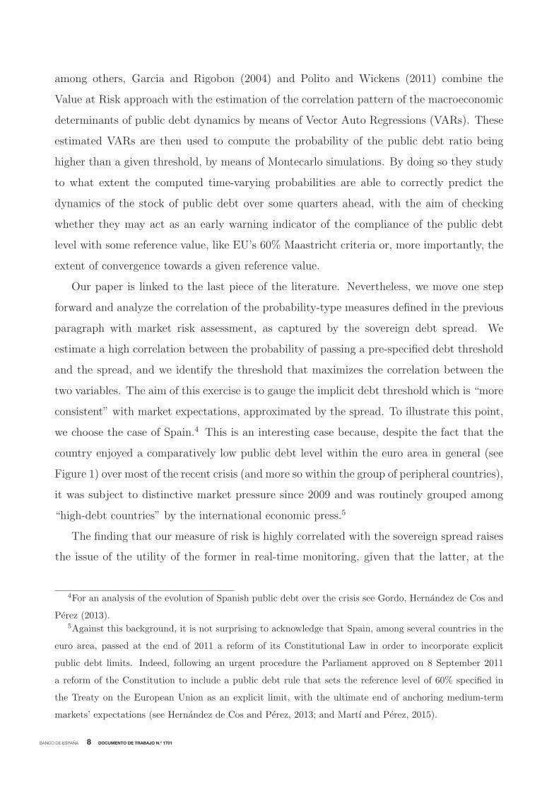
Figure 2: The evolution of Spanish public debt: 1970-2015.
1970 1975 1980 1985 1990 1995 2000 2005 2010 201510
20
30
40
50
60
70
80
90
100
Public debt, Spain
terms, the Spanish public debt-to-GDP ratio represented in 2012 about 95% of the euro area
ratio, similar to its relative level in 1996, but it outpaced it in 2014.
The rest of the paper is organized as follows. In Section 2 we describe the evolution of
public debt in Spain in the past few decades and provide some stylized facts. In Section 3
we discuss the data and the methodology used in the empirical analysis, while in Section 4
we discuss the main results. Finally, in Section 5 we present some conclusions.
2 Some stylized facts
In the case of Spain, as can be seen in Figure 2 the maximum level of debt as a percent of
GDP in the period 1970-2007 was reached in 1996 (65.6% of GDP). After the 1996 maximum,
public debt entered into a downward path until reaching a minimum of 35.5% in 2007. In the
period 2008-2014, nevertheless, debt increased substantially to reach 99.3%, the maximum
of the time series in the period 1970-2014, to marginally fall in 2015 to 99.2%. In relative
BANCO DE ESPAÑA 11 DOCUMENTO DE TRABAJO N.º 1701
From a backward looking perspective, it is apparent that Spanish public debt increased in
times of economic recession, but showed a significant downward rigidity in post-crisis times,
at least until the mid 1990s. Debt remained stable as a ratio to GDP during the 1970s.
Between 1980 and 1987 public debt increased by close to 30 percentage points of GDP, and
got stabilized at 1987’s level till 1991. This was the starting point for the second big increase
in the sample period analyzed, as the outburst of the 1993 crisis pushed upwards public debt
again, in such a way that the stock of government debt increased by some 25 percentage
points between 1992 and 1996. This hysteresis-like behavior witnessed over the decade and
a half that started in 1980 was curbed in the subsequent 1997-2007 period. In the latter
10-year period, sovereign debt was reduced by above 25 percentage points of GDP, only to
increase again substantially in the last part of the sample.
It is worth looking at the prolonged episode of debt reduction that started in the late
1990, and the subsequent increase in debt, through the lenses of the government budget
constraint. Let Yt be real GDP at t and let Dt be the real value of government debt. The
government budget constraint accounts for how the nominal interest rate it, net inflation
πt, net growth in real GDP, gdpt, the net-of-interest deficit as a percent of Yt, deft, and
the deficit-debt adjustment, DDAt combine to determine the evolution of the government
debt-to-GDP-ratio,
Dt
Yt
=1 + it
(1 + πt) (1 + gdpt)
Dt−1Yt−1
+ deft +DDAt
Yt
(1)
primary balance contributed to an average debt reduction of 2.9 percentage points per year,
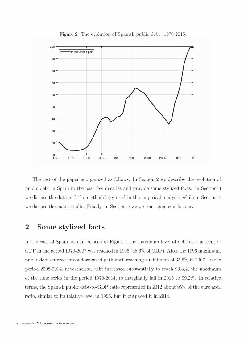
With this decomposition at hand it is possible to analyze the determinants of changes in
the debt-to-GDP ratio. In the upper panel of Figure 3 we decompose these determinants for
each year over the period 1996-2015. Focusing in a first stage in the period 1996-2007, the
were the nominal yield it and the real stock of debtDt are averages of pertinent objects across
terms to maturity. A standard, approximated version, suitable for accounting decomposition
of the fundamental determinants of debt, takes the form
Dt
Yt
=Dt−1Yt−1
+ (it − πt − gdpt)Dt−1Yt−1
+ deft +DDAt
Yt
(2)

BANCO DE ESPAÑA 12 DOCUMENTO DE TRABAJO N.º 1701
Figure 3: The determinants of the change in the Spanish public debt-to-GDP ratio.
Year-by-year changes
Cumulative changes
BANCO DE ESPAÑA 13 DOCUMENTO DE TRABAJO N.º 1701
an amount larger in size than the average contribution of real GDP (2.0 percentage points per
year on average) and inflation (1.8 points per year on average). These three positive factors
were partly compensated by an average 0.7 points per year debt-increasing contribution
stemming from deficit-debt adjustments, and the interest payments, that amounted to some
2.9% of GDP per year on average. As regards the 2008-2015 period, the sizeable increase in
debt was basically due to the worsened primary balance (5.3 pp per year), interest payments
(2.5 pp per year), and the adverse contribution of deficit-debt adjustments. To reinforce our
exposition, in the lower panel of Figure 3, in turn, we show the same information as before,
but cumulated, i.e. calculated by means of equation:
Dt
Yt
=Dt−τYt−τ
+τ−1∑s=0
[(it−s − πt−s − gdpt−s)
Dt−s−1Yt−s−1
+ deft−s +DDAt−sYt−s
](3)
Between 1996 and 2007, the 26 percentage points of public debt reduction can be broken
down as follows: (i) 35 percentage points of reduction due to the adjustment of the primary
balance; (ii) 23.9 points of reduction due to favorable real GDP growth; (iii) 21.6 percentage
points of reduction due to inflation; (iv) these three factors more than compensated the
increase of 35 points due to the interest payments during the period, and the 7.9 percentage
points due to the deficit-debt adjustments. On the contrary, in the course of the eight years
that span from 2008 to 2015, the abrupt reversal of all positive factors, most notably the
significant primary deficits, undid the results of the 1997-2007 consolidation period.
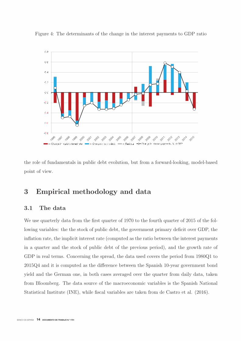
In the most recent period, the debt-increasing contribution of the interest burden veils a
favorable evolution of the implicit interest rate. Interestingly, implicit interest rate dynamics,
that averages interest rates of newly issued debt, including that refinanced, and rates of non-
maturing debt issued in the past, contributed to contain the increase in the public debt
ratio in 2008, 2009 and 2010, only turning to a positive contribution in 2011, when rates
at issuance increased substantially. The effect of ECB’s monetary policy measures on the
interest burden of the government becomes clear in the last part of the sample (see Figure
4).
After this brief backward-looking description of the contributions of the main determi-
nants of public debt to its evolution, in the subsequent Section we turn to the analysis of
BANCO DE ESPAÑA 14 DOCUMENTO DE TRABAJO N.º 1701
Figure 4: The determinants of the change in the interest payments to GDP ratio
the role of fundamentals in public debt evolution, but from a forward-looking, model-based
point of view.
3 Empirical methodology and data
3.1 The data
We use quarterly data from the first quarter of 1970 to the fourth quarter of 2015 of the fol-
lowing variables: the the stock of public debt, the government primary deficit over GDP, the
inflation rate, the implicit interest rate (computed as the ratio between the interest payments
in a quarter and the stock of public debt of the previous period), and the growth rate of
GDP in real terms. Concerning the spread, the data used covers the period from 1980Q1 to
2015Q4 and it is computed as the difference between the Spanish 10-year government bond
yield and the German one, in both cases averaged over the quarter from daily data, taken
from Bloomberg. The data source of the macroeconomic variables is the Spanish National
Statistical Institute (INE), while fiscal variables are taken from de Castro et al. (2016).
BANCO DE ESPAÑA 15 DOCUMENTO DE TRABAJO N.º 1701
3.2 Outline of the methodology
The approach to assess the dynamics and sustainability of public debt is based on the
sequential estimation of a Vector autoregression model, updated each period. As claimed
recently by Polito and Wickens (2011) this is instrumental for the problem at hand in that
it exploits the well-documented advantages of time-series models for forecasting in the short
run (see e.g. Stock and Watson, 2001), and also due to the fact that time-series models tend
to give better forecasts than structural models, particularly in the presence of structural
breaks (see e.g. Clements and Hendry, 2005). Even though we take an agnostic view and
estimate unrestricted VARs (structural models can be written as restricted VARs), we use
the theory to guide our selection of variables. In particular we use the government budget
constraint, as in (1) to select the variables to be included in the analysis.
More in detail, the procedure consists of the following steps. First, given an initial sample
size, a VAR is estimated using the variables that enter into the public debt equation, which in
its simplest form are: the ratio of the primary public deficit over GDP, the nominal interest
rate, the inflation rate and the growth rate of GDP. Second, given the estimated parameters
of the VAR and the corresponding variance-covariance matrix of the errors, a large number
of Monte-Carlo simulations are performed to obtain a large number of realizations of the
innovations and the associated realizations of the macroeconomic fundamentals of the debt
equation. This step entails the computation of the implied debt-to-GDP ratio for different
time horizons depending on the criteria of interest, where the period-by-period government
budget constraint, expressed as a ratio to total GDP takes its non-linear form as in (1).
The procedure can be applied sequentially and allows for the calculation of the proba-
bilistic distribution of the debt ratio for each quarter of the projection. Notice that at each
point in time t the procedure uses the macroeconomic data available up to t − 1 which are
the initial conditions of the relevant variables from which the simulated paths depart, and
consequently the exercise can be used to out-of-sample monitor the evolution of public debt
both in the short and the long term.

BANCO DE ESPAÑA 16 DOCUMENTO DE TRABAJO N.º 1701
3.3 VAR model
The first step of the approach entails the sequential estimation of a standard Vector Autor-
regression Model of the following form
Yt = μy + βt+ B(L)Yt−1 + Ut. (4)
where
Yt = (gdpt, πt, it, deft) (5)
μy and t deterministic terms (constants and trends), and Ut is the vector of reduced-form
residuals which are assumed to be distributed according to a multinomial distribution with
zero mean and covariance matrix Ω, i.e. Ut ∼ N(0,Ω). In order to allow for enough
observations at the beginning of the sample, the sequence of models is estimated over a
rolling window, with the initial sample being 1970Q2-1993Q4. Then, one quarter is added
at a time until reaching the whole sample (1970Q2-2015Q4).
3.4 The empirical distribution function of debt levels
The sequential estimation of the VAR and the computation of the simulated paths for public
debt generates, at each point in time, an empirical distribution function of debt levels. This
distribution function, that also depends on the simulation horizon, can be used to monitor
the evolution of public debt in both the short and the long term by computing the corre-
sponding moments of the simulated data. We denote as F Tt (d | It−1) the empirical cumulative
distribution function of debt realizations of length T conditional on the information available
up to period t− 1 (It−1, composed of past data and the estimated parameter coefficients of
the VAR model)
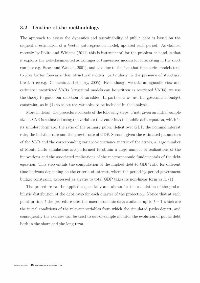
For illustrative purposes Figure 5 displays the cumulative distribution of debt at different
simulation spans (one quarter, one year and two years) when the associated VAR is estimated
with data until 2011Q4 and with data up to 2015Q4. Notice that at short simulation’s
horizons, debt outcomes are distributed tightly around the mean and as the projection
horizon lengthens, uncertainty increases in such a way that the distribution becomes more fat-
tailed and more extreme outcomes cannot be ruled out. Interestingly, public debt simulations
BANCO DE ESPAÑA 17 DOCUMENTO DE TRABAJO N.º 1701
Figure 5: Empirical CDF with alternative information sets.
With information up to 2011Q4 With information up to 2015Q4
65 70 75 80 85 90 95 100 105 1100
0.1
0.2
0.3
0.4
0.5
0.6
0.7
0.8
0.9
1
1 quarter1 year2 years
75 80 85 90 95 100 105 110 115 1200
0.1
0.2
0.3
0.4
0.5
0.6
0.7
0.8
0.9
1
1 quarter1 year2 years
performed with information up to the end of 2011 anticipated an increase of debt at all
horizons, while for the exercise performed with the sample up to 2015Q4 there is more
heterogeneity, with a non-negligible set of simulated paths indicating a reduction of public
debt.
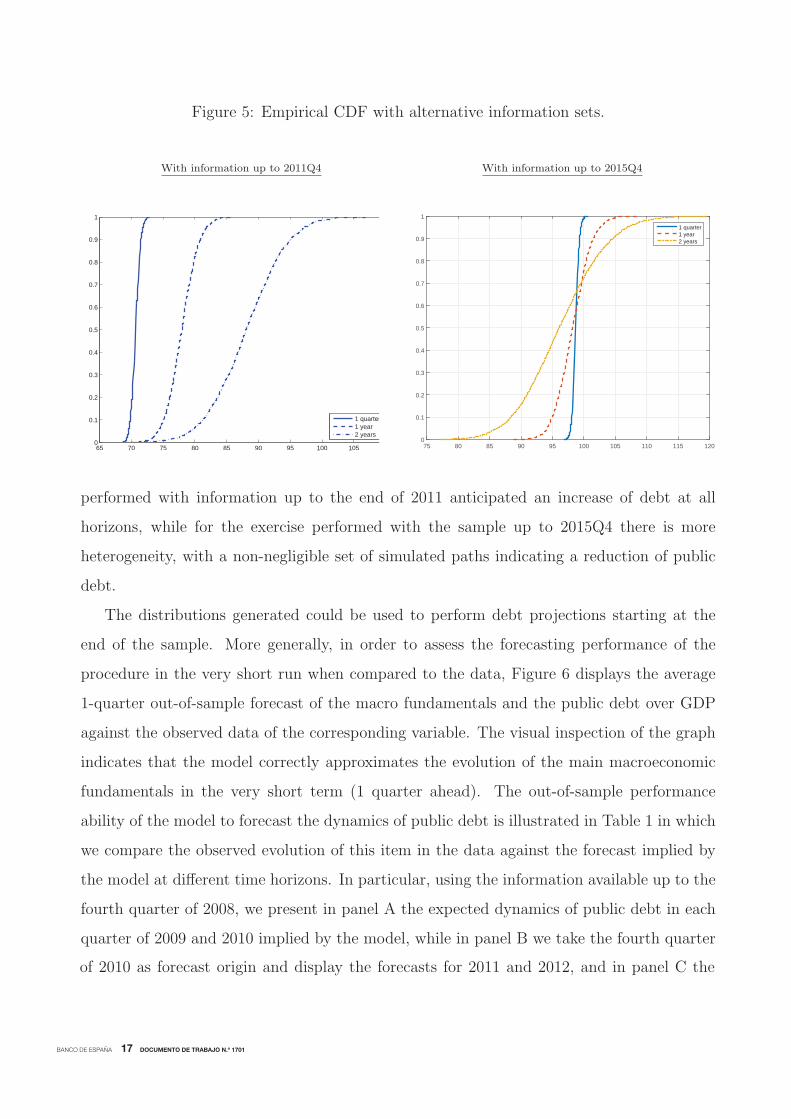
The distributions generated could be used to perform debt projections starting at the
end of the sample. More generally, in order to assess the forecasting performance of the
procedure in the very short run when compared to the data, Figure 6 displays the average
1-quarter out-of-sample forecast of the macro fundamentals and the public debt over GDP
against the observed data of the corresponding variable. The visual inspection of the graph
indicates that the model correctly approximates the evolution of the main macroeconomic
fundamentals in the very short term (1 quarter ahead). The out-of-sample performance
ability of the model to forecast the dynamics of public debt is illustrated in Table 1 in which
we compare the observed evolution of this item in the data against the forecast implied by
the model at different time horizons. In particular, using the information available up to the
fourth quarter of 2008, we present in panel A the expected dynamics of public debt in each
quarter of 2009 and 2010 implied by the model, while in panel B we take the fourth quarter
of 2010 as forecast origin and display the forecasts for 2011 and 2012, and in panel C the
BANCO DE ESPAÑA 18 DOCUMENTO DE TRABAJO N.º 1701
Figure 6: Data (solid lines) versus one-quarter-ahead forecasts (dashed lines).
70Q2 77Q4 85Q2 92Q4 00Q2 07Q4 15Q2-2
-1
0
1
2
3REAL GDP (% growth)
EstimatedActual
70Q2 77Q4 85Q2 92Q4 00Q2 07Q4 15Q2-1
0
1
2
3
4
5
6INFLATION (% growth)
70Q2 77Q4 85Q2 92Q4 00Q2 07Q4 15Q2-5
0
5
10
15PRIMARY DEFICIT (percent of GDP)
70Q2 77Q4 85Q2 92Q4 00Q2 07Q4 15Q20
0.5
1
1.5
2
2.5
3IMPLICIT INTEREST RATE (percent of GDP)
6The results are available from the authors upon request.
projections with information up to 2013Q4. As mentioned before, the standard deviation of
the forecast increases at longer horizons. Beyond this illustrative forecast paths, the short-,
medium-, and long-term projections of the VARs beat simple benchmark models like the
standard random walk and univariate alternatives to extrapolate public debt.6
3.5 The risk measure of public debt and the “prudent” medium-
term level
Apart from the calculation of forecasts, the time dependent empirical distribution function
can also be used to monitor the expected evolution of public debt in probabilistic terms. In

BANCO DE ESPAÑA 19 DOCUMENTO DE TRABAJO N.º 1701
Table 1: Public debt forecasts at the beginning of the economic crisis (2008Q1), in the midst
of the euro area sovereign debt crisis (2010Q4), and in the recovery phase (2013Q4).
Panel A. Forecast origin 2008Q4.
2009 2010
Q1 Q2 Q3 Q4 Q1 Q2 Q3 Q4
Actual 42.6 46.7 50.4 52.4 55.3 56.5 58.4 59.5
Forecasts: Minimum 39.7 46.0 52.1 55.6 55.2 55.5 53.7 52.6
Forecasts: Mean 40.7 49.0 56.7 62.2 63.9 64.7 66.8 70.1
Forecasts: Maximum 41.6 51.9 61.0 69.2 75.0 75.6 81.9 88.7
Forecast: Standard deviation 0.26 0.66 1.15 1.77 2.38 3.02 3.84 4.76
Panel B. Forecast origin 2010Q4.
2011 2012
Q1 Q2 Q3 Q4 Q1 Q2 Q3 Q4
Actual 62.5 66.6 68.8 69.6 72.5 76.8 79.6 81.2
Forecasts: Minimum 60.4 64.3 67.5 71.6 72.7 72.5 75.1 66.8
Forecasts: Mean 61.7 67.6 73.5 78.6 82.7 87.8 95.3 92.6
Forecasts: Maximum 62.9 70.4 78.5 86.2 94.0 103.8 115.9 116.5
Forecast: Standard deviation 0.34 0.81 1.43 2.19 3.04 4.07 5.34 6.14
Panel C. Forecast origin 2013Q4.
2014 2015
Q1 Q2 Q3 Q4 Q1 Q2 Q3 Q4
Actual 95.1 97.6 98.3 98.4 98.5 98.9 98.5 98.5
Forecasts: Minimum 93.7 93.6 93.9 90.8 87.7 82.7 75.1 73.8
Forecasts: Mean 95.5 97.7 99.8 99.6 99.5 96.6 95.5 95.6
Forecasts: Maximum 97.3 102.2 106.6 110.1 113.2 112.3 117.2 120.3
Forecast: Standard deviation 0.50 1.12 1.84 2.66 3.56 4.32 5.29 6.23
Note: Excluding deficit-debt adjustments. Public debt figures in each quarter are normalized by nominal GDP in that
quarter, annualized. Thus, the so-computed ratios are different from the standard presentation in which the sum of four
consecutive quarters up to the current one is taken.
BANCO DE ESPAÑA 20 DOCUMENTO DE TRABAJO N.º 1701
Table 2: Correlations between the probability and the spread
Time span
10 years 5 years 1 year
1994Q1-2015Q4 0.74 0.69 0.51
1994Q1-2007Q4 0.84 0.72 0.29
1999Q1-2013Q2 0.79 0.74 0.53
particular, given the distribution function, it is possible to compute the probability of public
debt being higher than a particular threshold θ some quarters ahead T , given the information
available at some point in time denoted as It−1. Notice that the sequence of probabilities will
be time dependent. Formally, at each point in time t the following probability is computed
pTt/t−1(θ) = P (d > θ | It−1) = 1− F Tt (θ | It−1) (6)
and the sequence of such probabilities {pTt/t−1(θ)} which will be denoted as P Tt/t−1(θ). As
suggested before, one possible way of summarizing the information provided by the time
dependent distribution function of public debt level is to compute the probability of ob-
serving a debt level above some threshold of interest which is deemed to be critical for its
sustainability. An example is the 60% public debt level of reference for the Stability and
Growth Pact and the Spanish Constitution. This exercise, in itself, is useful to monitor
compliance with fiscal rules or simulate alternative scenarios of interest, and as such is used
in the related literature.
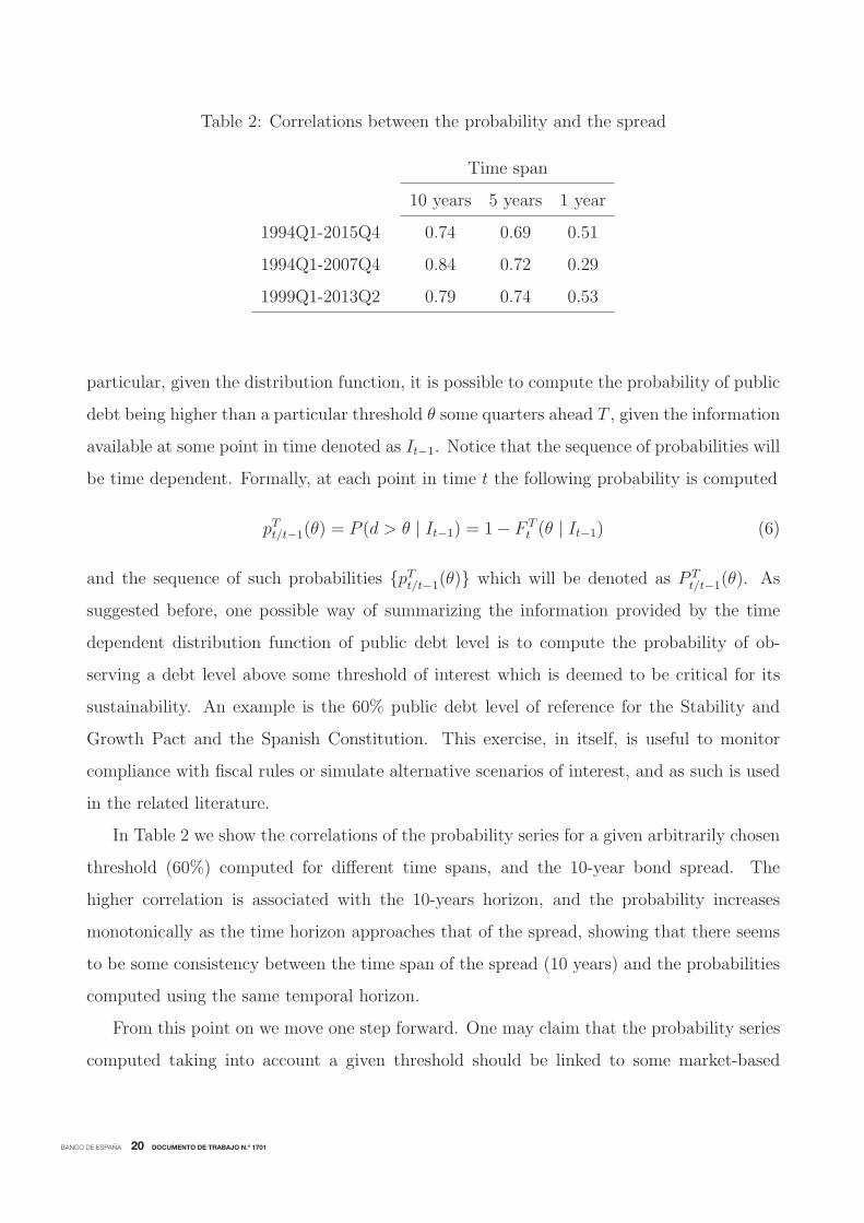
In Table 2 we show the correlations of the probability series for a given arbitrarily chosen
threshold (60%) computed for different time spans, and the 10-year bond spread. The
higher correlation is associated with the 10-years horizon, and the probability increases
monotonically as the time horizon approaches that of the spread, showing that there seems
to be some consistency between the time span of the spread (10 years) and the probabilities
computed using the same temporal horizon.
From this point on we move one step forward. One may claim that the probability series
computed taking into account a given threshold should be linked to some market-based

BANCO DE ESPAÑA 21 DOCUMENTO DE TRABAJO N.º 1701
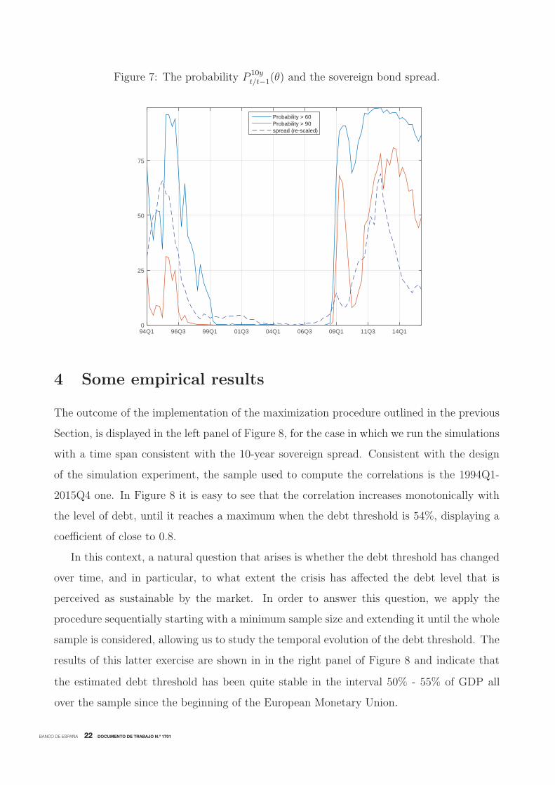
measure of risk in the market for public debt (Garcıa and Rigobon, 2004). In our framework
this is illustrated in Figure 7, were we plot the recursive probability obtained at each point
in time (as measured by the time axis) of breaching the 60% of GDP debt threshold in 10
years from the forecasts origin, i.e. P 10yt/t−1(60). Interestingly, just by simple inspection some
close correlation among the two series becomes evident.
Thus, it seems natural to study the linkages between the measure of risk calculated in
(6) and the standard indicator of risk, namely the sovereign bond spread. In this fashion,
we calculate the threshold that maximizes the correlation between our risk measure and
the sovereign bond spread in order to gauge the implicit debt threshold which is the most
consistent with market expectations approximated by the spread. Formally,
θ∗ = argmaxθ
corr(P Tt/t−1(θ), St) (7)
i.e. conditional on the information set available at t, It−1, we solve (7) to get the debt
threshold, θ∗, relevant for market participants that use as a reference the time horizon T .
This debt threshold θ∗ can be viewed as the one that shapes market participants expectations
about the evolution of public finances and then as a market-based index of debt sustainability.
As such, this does not imply that debt reaches its “maximum affordable” level, as defined
by the fiscal limit (i.e., “...the point beyond which taxes and government expenditures can
no longer adjust to stabilize the value of government debt...”, Leeper and Walker, 2011),
but rather that the debt ratio enters in a region in which the degree of vulnerability of
public finances becomes high, possibly with an associated non-negligible probability of debt
becoming under stress so that the price of bonds drops dramatically to allow for a risk
premium. In that sense, θ∗ is more associated to the lower limit of the probability distribution
of the fiscal limit itself, beyond which the debt ratio displays a small but non negligible
probability of reaching the fiscal limit, thus triggering a non linear response of the spread
(Bi, 2012). In the current circumstance in the euro zone, though, such a response is likely
to be muted by the fact that a major player in the sovereign debt market is present (i.e. the
ECB), as compared to normal periods in which governments are forced to access the market
to cover their financing needs.
BANCO DE ESPAÑA 22 DOCUMENTO DE TRABAJO N.º 1701
Figure 7: The probability P 10yt/t−1(θ) and the sovereign bond spread.
94Q1 96Q3 99Q1 01Q3 04Q1 06Q3 09Q1 11Q3 14Q10
25
50
75
Probability > 60Probability > 90spread (re-scaled)
4 Some empirical results
The outcome of the implementation of the maximization procedure outlined in the previous
Section, is displayed in the left panel of Figure 8, for the case in which we run the simulations
with a time span consistent with the 10-year sovereign spread. Consistent with the design
of the simulation experiment, the sample used to compute the correlations is the 1994Q1-
2015Q4 one. In Figure 8 it is easy to see that the correlation increases monotonically with
the level of debt, until it reaches a maximum when the debt threshold is 54%, displaying a
coefficient of close to 0.8.
In this context, a natural question that arises is whether the debt threshold has changed
over time, and in particular, to what extent the crisis has affected the debt level that is
perceived as sustainable by the market. In order to answer this question, we apply the
procedure sequentially starting with a minimum sample size and extending it until the whole
sample is considered, allowing us to study the temporal evolution of the debt threshold. The
results of this latter exercise are shown in in the right panel of Figure 8 and indicate that
the estimated debt threshold has been quite stable in the interval 50% - 55% of GDP all
over the sample since the beginning of the European Monetary Union.

BANCO DE ESPAÑA 23 DOCUMENTO DE TRABAJO N.º 1701
Figure 8: The “prudent” public debt threshold
Correlation between the sovereign spread Time variation of the public debt threshold
and the different public debt thresholds that maximizes the correlation with the spread
debt limit20 30 40 50 60 70 80 90 100
corr
elat
ion
0
0.1
0.2
0.3
0.4
0.5
0.6
0.7
0.8
0.9
Quarters00Q2 02Q2 04Q2 06Q2 08Q2 10Q2 12Q2 14Q2
Per
cent
of G
DP
40
45
50
55
60
65
70
Public debt threshold
7In this respect, one could nowcast Yt for the current quarter t by means of monthly indicators, and
update Pt/t−1 with more timely information.
In a final exercise we test whether or not the probability measure Granger-causes the
market risk indicator, St. To do so, we run regressions of the kind:
St = Γ(L) St−1 + Φ(L) P Tt/t−1(θ) + εt (8)
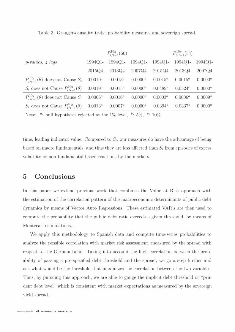
We show some selected results in Table 3, for the computed probabilities of breaching
the 60% limit. The table presents Granger Causality tests between St and P 10yt/t−1(60), and
between St and P 10yt/t−1(54). We show the specification for 4 lags (the results are robust to this
choice) and different sample sizes. In addition, we show in the table the tests for P 10yt+1/t(60)
and P 10yt+1/t(54). This is warranted as the leaded variable is contemporaneous with respect to
St from the point of view of the moment in time in which it is known to the analyst. This
is so because the measure P 10yt/t−1(θ) is the probability computed for quarter t with data and
estimated parameters up to t − 1, and as a consequence, its information content is lagged
with respect to St.7 From the results in the table, P 10y
t/t−1(60) Granger-Causes St, and also
when P 10yt+1/t(θ) is forwarded, for all specifications (i.e. the null hypothesis of no causation
gets rejected). The results in Table 3 indicate that the probability measures contains real-
BANCO DE ESPAÑA 24 DOCUMENTO DE TRABAJO N.º 1701
Table 3: Granger-causality tests: probability measures and sovereign spread.
P 10yt/t−1(60) P 10y
t/t−1(54)
p-values, 4 lags 1994Q1- 1994Q1- 1994Q1- 1994Q1- 1994Q1- 1994Q1-
2015Q4 2013Q4 2007Q4 2015Q4 2013Q4 2007Q4
P 10yt/t−1(θ) does not Cause St 0.0010a 0.0013a 0.0000a 0.0015a 0.0015a 0.0000a
St does not Cause P 10yt/t−1(θ) 0.0019a 0.0015a 0.0000a 0.0489b 0.0524c 0.0000a
P 10yt/t−1(θ) does not Cause St 0.0006a 0.0016a 0.0000a 0.0003a 0.0006a 0.0009a
St does not Cause P 10yt/t−1(θ) 0.0013a 0.0007a 0.0000a 0.0394b 0.0337b 0.0000a
Note: a: null hypothesis rejected at the 1% level, b: 5%, c: 10%.
ask what would be the threshold that maximizes the correlation between the two variables.
Thus, by pursuing this approach, we are able to gauge the implicit debt threshold or “pru-
dent debt level” which is consistent with market expectations as measured by the sovereign
yield spread.
time, leading indicator value. Compared to St, our measures do have the advantage of being
based on macro fundamentals, and thus they are less affected than St from episodes of excess
volatility or non-fundamental-based reactions by the markets.
5 Conclusions
In this paper we extend previous work that combines the Value at Risk approach with
the estimation of the correlation pattern of the macroeconomic determinants of public debt
dynamics by means of Vector Auto Regressions. These estimated VAR’s are then used to
compute the probability that the public debt ratio exceeds a given threshold, by means of
Montecarlo simulations.
We apply this methodology to Spanish data and compute time-series probabilities to
analyze the possible correlation with market risk assessment, measured by the spread with
respect to the German bond. Taking into account the high correlation between the prob-
ability of passing a pre-specified debt threshold and the spread, we go a step further and

BANCO DE ESPAÑA 25 DOCUMENTO DE TRABAJO N.º 1701
References
Aiyagari S. R. and E. R. McGrattan (1998), “The Optimum Quantity of Debt”, Journal of
Monetary Economics, 42, 447-469.
Bi, H. (2012), “Sovereign Default Risk Premia, Fiscal Limits and Fiscal Policy”, European
Economic Review, 56, pp. 389–410.
Bi, H. and E. Leeper (2013), “Analyzing Fiscal Sustainability”. Bank of Canada Working
Paper, 2013-27.
Collard, F., M. Habib and J. Rochet (2015), “Sovereign Debt Sustainability in Advanced
Economies”. Journal of the European Economic Association, 13, pp. 381-420.
de Castro, F., F. Martı, A. Montesinos, J. J. Perez, A. J. Sanchez-Fuentes (2016), “A quar-
terly fiscal database fit for macroeconomic analysis”, mimeo, Bank of Spain. Previous
version available as Bank of Spain Working Paper 1408.
Daniel, C. B. and C. Shiamptanis (2013), “Pushing the limit? Fiscal policy in the European
Monetary Union”, Journal of Economic Dynamics and Control, 37, pp. 2307-2321.
Desbonnet, A. and S. Kankamge (2007), “Public debt and aggregate risk”, Documents de
travail du Centre d’Economie de la Sorbonne 2007-42.
Fall, F. and J.-M. Fournier (2015), “Macroeconomic uncertainties, prudent debt targets
and fiscal rules”, OECD Economics Department Working Papers, no 1230.
Floden M. (2001), “The effectiveness of government debt and transfers as insurance”, Jour-
nal of Monetary Economics, 48, 81-108.
Ghosh, A., J. Kim, E. Mendoza, J- Ostry and M. Qureshi (2015), “Fiscal Fatigue, Fiscal
Space and Debt Sustainability in Advanced Economies”, The Economic Journal, 123,
pp. F4F30.
Gordo, L., Hernandez de Cos, P. and J. J. Perez (2013), “Developments in Spanish public
debt since the start of the crisis”. Bank of Spain Economic Bulletin, July-August, pp.
19-36.

BANCO DE ESPAÑA 26 DOCUMENTO DE TRABAJO N.º 1701
Hernandez de Cos, P. and J. J. Perez (2013), “The new budgetary stability law”. Bank of
Spain Economic Bulletin, April, pp. 13-25.
Hiebert, P., J. J. Perez and M. Rostagno (2009), “The trade-off between public debt reduc-
tion and automatic stabilisation”, Economic Modelling, 26, pp. 464-472.
Kleven H.J. and C.T. Kreiner (2003), “The role of taxes as automatic destabilizers in New
Keynesian economics”, Journal of Public Economics, 87, pp. 1123-1136.
Leeper, E. M. and T. B. Walker (2011), “Fiscal Limits in Advanced Economies”, NBER
Working Papers 16819, National Bureau of Economic Research, Inc.
Martı, F. and J. J. Perez (2015), “Spanish public finances through the financial crisis”,
Fiscal Studies, 36, pp. 527-554.
Mendoza, E. and P. M. Oviedo (2006), “Fiscal Policy and Macroeconomic Uncertainty in
Developing Countries: The Tale of the Tormented Insurer”, NBER Working Papers
12586, National Bureau of Economic Research, Inc.
Polito, V.and M. Wichens (2011), “A model-based indicator of the fiscal stance”, European
Economic Review, 56, pp. 526-551.
Woodford M. (1990), “Public Debt as Private Liquidity”, American Economic Review, 80,
pp. 382-388.
BANCO DE ESPAÑA PUBLICATIONS
WORKING PAPERS
1530 CRISTINA FERNÁNDEZ and PILAR GARCÍA PEREA: The impact of the euro on euro area GDP per capita.
1531 IRMA ALONSO ÁLVAREZ: Institutional drivers of capital fl ows.
1532 PAUL EHLING, MICHAEL GALLMEYER, CHRISTIAN HEYERDAHL-LARSEN and PHILIPP ILLEDITSCH: Disagreement
about infl ation and the yield curve.
1533 GALO NUÑO and BENJAMIN MOLL: Controlling a distribution of heterogeneous agents.
1534 TITO BOERI and JUAN F. JIMENO: The unbearable divergence of unemployment in Europe.
1535 OLYMPIA BOVER: Measuring expectations from household surveys: new results on subjective probabilities of future
house prices.
1536 CRISTINA FERNÁNDEZ, AITOR LACUESTA, JOSÉ MANUEL MONTERO and ALBERTO URTASUN: Heterogeneity
of markups at the fi rm level and changes during the great recession: the case of Spain.
1537 MIGUEL SARMIENTO and JORGE E. GALÁN: The infl uence of risk-taking on bank effi ciency: evidence from Colombia.
1538 ISABEL ARGIMÓN, MICHEL DIETSCH and ÁNGEL ESTRADA: Prudential fi lters, portfolio composition and capital ratios
in European banks.
1539 MARIA M. CAMPOS, DOMENICO DEPALO, EVANGELIA PAPAPETROU, JAVIER J. PÉREZ and ROBERTO RAMOS:
Understanding the public sector pay gap.
1540 ÓSCAR ARCE, SAMUEL HURTADO and CARLOS THOMAS: Policy spillovers and synergies in a monetary union.
1601 CHRISTIAN CASTRO, ÁNGEL ESTRADA and JORGE MARTÍNEZ: The countercyclical capital buffer in Spain:
an analysis of key guiding indicators.
1602 TRINO-MANUEL ÑÍGUEZ and JAVIER PEROTE: Multivariate moments expansion density: application of the dynamic
equicorrelation model.
1603 ALBERTO FUERTES and JOSÉ MARÍA SERENA: How fi rms borrow in international bond markets: securities regulation
and market segmentation.
1604 ENRIQUE ALBEROLA, IVÁN KATARYNIUK, ÁNGEL MELGUIZO and RENÉ OROZCO: Fiscal policy and the cycle
in Latin America: the role of fi nancing conditions and fi scal rules.
1605 ANA LAMO, ENRIQUE MORAL-BENITO and JAVIER J. PÉREZ: Does slack infl uence public and private labour
market interactions?
1606 FRUCTUOSO BORRALLO, IGNACIO HERNANDO and JAVIER VALLÉS: The effects of US unconventional monetary
policies in Latin America.
1607 VINCENZO MERELLA and DANIEL SANTABÁRBARA: Do the rich (really) consume higher-quality goods? Evidence from
international trade data.
1608 CARMEN BROTO and MATÍAS LAMAS: Measuring market liquidity in US fi xed income markets: a new synthetic
indicator.
1609 MANUEL GARCÍA-SANTANA, ENRIQUE MORAL-BENITO, JOSEP PIJOAN-MAS and ROBERTO RAMOS: Growing like
Spain: 1995-2007.
1610 MIGUEL GARCÍA-POSADA and RAQUEL VEGAS: Las reformas de la Ley Concursal durante la Gran Recesión.
1611 LUNA AZAHARA ROMO GONZÁLEZ: The drivers of European banks’ US dollar debt issuance: opportunistic funding
in times of crisis?
1612 CELESTINO GIRÓN, MARTA MORANO, ENRIQUE M. QUILIS, DANIEL SANTABÁRBARA and CARLOS TORREGROSA:
Modelling interest payments for macroeconomic assessment.
1613 ENRIQUE MORAL-BENITO: Growing by learning: fi rm-level evidence on the size-productivity nexus.
1614 JAIME MARTÍNEZ-MARTÍN: Breaking down world trade elasticities: a panel ECM approach.
1615 ALESSANDRO GALESI and OMAR RACHEDI: Structural transformation, services deepening, and the transmission
of monetary policy.
1616 BING XU, ADRIAN VAN RIXTEL and HONGLIN WANG: Do banks extract informational rents through collateral?
1617 MIHÁLY TAMÁS BORSI: Credit contractions and unemployment.

1618 MIHÁLY TAMÁS BORSI: Fiscal multipliers across the credit cycle.
1619 GABRIELE FIORENTINI, ALESSANDRO GALESI and ENRIQUE SENTANA: A spectral EM algorithm for dynamic
factor models.
1620 FRANCISCO MARTÍ and JAVIER J. PÉREZ: Spanish public fi nances through the fi nancial crisis.
1621 ADRIAN VAN RIXTEL, LUNA ROMO GONZÁLEZ and JING YANG: The determinants of long-term debt issuance by
European banks: evidence of two crises.
1622 JAVIER ANDRÉS, ÓSCAR ARCE and CARLOS THOMAS: When fi scal consolidation meets private deleveraging.
1623 CARLOS SANZ: The effect of electoral systems on voter turnout: evidence from a natural experiment.
1624 GALO NUÑO and CARLOS THOMAS: Optimal monetary policy with heterogeneous agents.
1625 MARÍA DOLORES GADEA, ANA GÓMEZ-LOSCOS and ANTONIO MONTAÑÉS: Oil price and economic growth:
a long story?
1626 PAUL DE GRAUWE and EDDIE GERBA: Stock market cycles and supply side dynamics: two worlds, one vision?
1627 RICARDO GIMENO and EVA ORTEGA: The evolution of infl ation expectations in euro area markets.
1628 SUSANA PÁRRAGA RODRÍGUEZ: The dynamic effect of public expenditure shocks in the United States.
1629 SUSANA PÁRRAGA RODRÍGUEZ: The aggregate effects of government incometransfer shocks - EU evidence.
1630 JUAN S. MORA-SANGUINETTI, MARTA MARTÍNEZ-MATUTE and MIGUEL GARCÍA-POSADA: Credit, crisis
and contract enforcement: evidence from the Spanish loan market.
1631 PABLO BURRIEL and ALESSANDRO GALESI: Uncovering the heterogeneous effects of ECB unconventional
monetary policies across euro area countries.
1632 MAR DELGADO TÉLLEZ, VÍCTOR D. LLEDÓ and JAVIER J. PÉREZ: On the determinants of fi scal non-compliance:
an empirical analysis of Spain’s regions.
1633 OMAR RACHEDI: Portfolio rebalancing and asset pricing with heterogeneous inattention.
1634 JUAN DE LUCIO, RAÚL MÍNGUEZ, ASIER MINONDO and FRANCISCO REQUENA: The variation of export prices
across and within fi rms.
1635 JUAN FRANCISCO JIMENO, AITOR LACUESTA, MARTA MARTÍNEZ-MATUTE and ERNESTO VILLANUEVA:
Education, labour market experience and cognitive skills: evidence from PIAAC.
1701 JAVIER ANDRÉS, JAVIER J. PÉREZ and JUAN A. ROJAS: Implicit public debt thresholds: an empirical exercise
for the case of Spain.
Unidad de Servicios AuxiliaresAlcalá, 48 - 28014 Madrid
E-mail: [email protected]