Implicit public debt thresholds: an empirical exercise for the case of ...

Implicit public debt thresholds: an empirical exercise for

the case of Spain∗

Javier Andres

Univ. of Valencia

Javier J. Perez

Banco de Espana

Juan A. Rojas

ESM

Abstract

We extend previous work that combines the Value at Risk approach with the es-

timation of the correlation pattern of the macroeconomic determinants of public debt

dynamics by means of Vector Auto Regressions (VARs). These estimated models are

used to compute the probability that the public debt ratio exceeds a given threshold,

by means of Montecarlo simulations. We apply this methodology to Spanish data and

compute time-series probabilities to analyze the possible correlation with market risk

assessment, measured by the spread with respect to the German bond. Taking into

account the high correlation between the probability of passing a pre-specified debt

threshold and the spread, we go a step further and ask what would be the threshold

that maximizes the correlation between the two variables. The aim of this exercise is to

gauge the implicit debt threshold or “prudent debt level” which is the most consistent

with market expectations as measured by the sovereign yield spread. The so-obtained

level is consistent with the medium-term debt-to-GDP ratio anchor of 60% of GDP.

JEL Classification: H63; H68; E61; E62.

Keywords: Public debt; early warning indicators; fiscal sustainability.

∗The views expressed in this paper are the authors’ and do not necessarily reflect those of the Bank

of Spain, the Eurosystem or the European Stability Mechanism (ESM). We thank the helpful comments of

participants at the following meetings: Banca d’Italia Public Finance WS (Rome, 2016), EEP (Girona, 2014),

IIPF (Taormina, 2013), EEA (Gothemburg, 2013), WGPFWS (Bratislava, 2012), WGEMmeeting (Brussels,

2012), and Public Finance WS at the EC (Brussels, 2011), in particular Alexander Mahle, Pietro Rizza,

Alberto Gonzalez-Pandiella and Lukas Reiss. Corresponding author: Javier J. Perez ([email protected]).

1

1 Introduction

This paper presents an empirical exercise that aims at highlighting the dependence of the

public debt level that a given country can afford or maintain in the medium-term on the

macroeconomic and fiscal fundamentals of the country. Some countries are able to maintain

a high level of public debt over long and sustained periods of time while keeping normal

access to the international markets, while others have to keep a significant public debt buffer

against adverse macroeconomic and fiscal developments. A standard result of the extant

literature is that public debt should act as a shock absorber to help smooth the response of

other budgetary variables, in particular to avoid drastic increases in tax rates or decreases in

spending in downturns. Nevertheless, this result is obtained under perfect access to markets

by the government. If a given government, on the contrary, were subject to market pressure

and limited market access, then even under a situation of economic distress a given country

may end up implementing a counter-cyclical fiscal consolidation plan.

In this regard, some empirical and theoretical literature suggest that a country-specific

“affordable” or “prudent” public debt level exist, beyond which a given country would be

more vulnerable and/or subject to a higher level of fiscal stress and market scrutiny.1 Ratio-

nal markets should be able to assess the evolution of fundamentals and thus impose tighter

debt limits on countries with weaker and/or more volatile fundamentals, in particular with

lower mean GDP growth rates or higher economics volatility.2 One particular branch of

the latter literature discusses the main determinants of the maximum level of debt that a

country can afford without defaulting, as well as the non-linear behavior of financing costs

once the debt to GDP ratio of a country approaches that level.3

The idea of a “prudent” government debt level has also been touched upon by the lit-

erature dealing with the analysis of public debt sustainability. In particular, among others,

1See e.g. Fall and Fournier (2015), and the references quoted therein. This literature is different, though

related, to that dealing with the optimality of public debt, as Woodford (1990), Aiyagari and McGrattan

(1998), Floden (2001), or Debonnet and Kankamge (2007).2See for example Mendoza and Oviedo (2006) or Hiebert, Perez and Rostagno (2009).3Along these lines one can classify the literature dealing with the fiscal limit (Bi, 2012, Bi and Leeper,

2013, Gosh et al., 2015, or Daniel and Shiamptanis (2013).) or that defining the “Maximum Sustainable

Debt ratio” (as in Collard, Habib and Rochet, 2016).

2

Garcia and Rigobon (2004) and Polito and Wickens (2011) combine the Value at Risk ap-

proach with the estimation of the correlation pattern of the macroeconomic determinants of

public debt dynamics by means of Vector Auto Regressions (VARs). These estimated VARs

are then used to compute the probability of the public debt ratio being higher than a given

threshold, by means of Montecarlo simulations. By doing so they study to what extent the

computed time-varying probabilities are able to correctly predict the dynamics of the stock

of public debt over some quarters ahead, with the aim of checking whether they may act as

an early warning indicator of the compliance of the public debt level with some reference

value, like EU’s 60% Maastricht criteria or, more importantly, the extent of convergence

towards a given reference value.

Our paper is linked to the last piece of the literature. Nevertheless, we move one step

forward and analyze the correlation of the probability-type measures defined in the previous

paragraph with market risk assessment, as captured by the sovereign debt spread. We

estimate a high correlation between the probability of passing a pre-specified debt threshold

and the spread, and we identify the threshold that maximizes the correlation between the

two variables. The aim of this exercise is to gauge the implicit debt threshold which is “more

consistent” with market expectations, approximated by the spread. To illustrate this point,

we choose the case of Spain.4 This is an interesting case because, despite the fact that the

country enjoyed a comparatively low public debt level within the euro area in general (see

Figure 1) over most of the recent crisis (and more so within the group of peripheral countries),

it was subject to distinctive market pressure since 2009 and was routinely grouped among

“high-debt countries” by the international economic press.5

The finding that our measure of risk is highly correlated with the sovereign spread raises

4For an analysis of the evolution of Spanish public debt over the period 2008-2012 see Gordo, Hernandez

de Cos and Perez (2013) and Delgado-Tellez et al. (2016).5Against this background, it is not surprising to acknowledge that Spain, among several countries in the

euro area, passed at the end of 2011 a reform of its Constitutional Law in order to incorporate explicit

public debt limits. Indeed, following an urgent procedure the Parliament approved on 8 September 2011

a reform of the Constitution to include a public debt rule that sets the reference level of 60% specified in

the Treaty on the European Union as an explicit limit, with the ultimate end of anchoring medium-term

markets’ expectations.

3

Figure 1: Evolution of the general government debt-to-GDP ratio in selected euro area

countries.

1995 2000 2005 2010 201520

40

60

80

100

120

140

FranceItalyGermanyEuro areaSpain

the issue of the utility of the former in real-time monitoring, given that the latter, at the

end of the day, is available on a daily basis. In this respect, we argue that the advantage of

complementing the standard analysis with the probability measures we compute is twofold.

First, it is a measure based on fundamentals, and thus not subject to market volatility.

Second, we show that our measures Granger-cause the information contained in the spread,

and thus, in a sense, do contain advanced information that is only reflected in the market

measures with some delay.

We conduct our empirical exercise for the period starting in the mid-1990s up until the

fourth quarter of 2015. Certainly, it is worth mentioning that the behaviour of the sovereign

spreads in the latter part of the sample (since 2013) is likely to have been influenced by

two key factors, beyond the standard determinants highlighted by the literature. First and

foremost, the introduction of non-standard monetary policy measures by the ECB, includ-

ing massive buy-outs of public debt. Second, the establishment of the European Stability

4

Figure 2: The evolution of Spanish public debt: 1970-2015.

1970 1975 1980 1985 1990 1995 2000 2005 2010 201510

20

30

40

50

60

70

80

90

100

Public debt, Spain

Mechanism as a backstop that intended to mute sovereign debt risks.

The rest of the paper is organized as follows. In Section 2 we describe the evolution of

public debt in Spain in the past few decades and provide some stylized facts. In Section 3

we discuss the data and the methodology used in the empirical analysis, while in Section 4

we discuss the main results. Finally, in Section 5 we present some conclusions.

2 Some stylized facts

As can be seen in Figure 2 the maximum level of debt as a percent of GDP in the period 1970-

2007 was reached in 1996 (65.6% of GDP). After the 1996 maximum, public debt entered

into a downward path until reaching a minimum of 35.5% in 2007. In the period 2008-2014,

nevertheless, debt increased substantially to reach 99.3%, the maximum of the time series

in the period 1970-2014, to marginally fall in 2015 to 99.2%. In relative terms, the Spanish

public debt-to-GDP ratio represented in 2012 about 95% of the euro area ratio, similar to

5

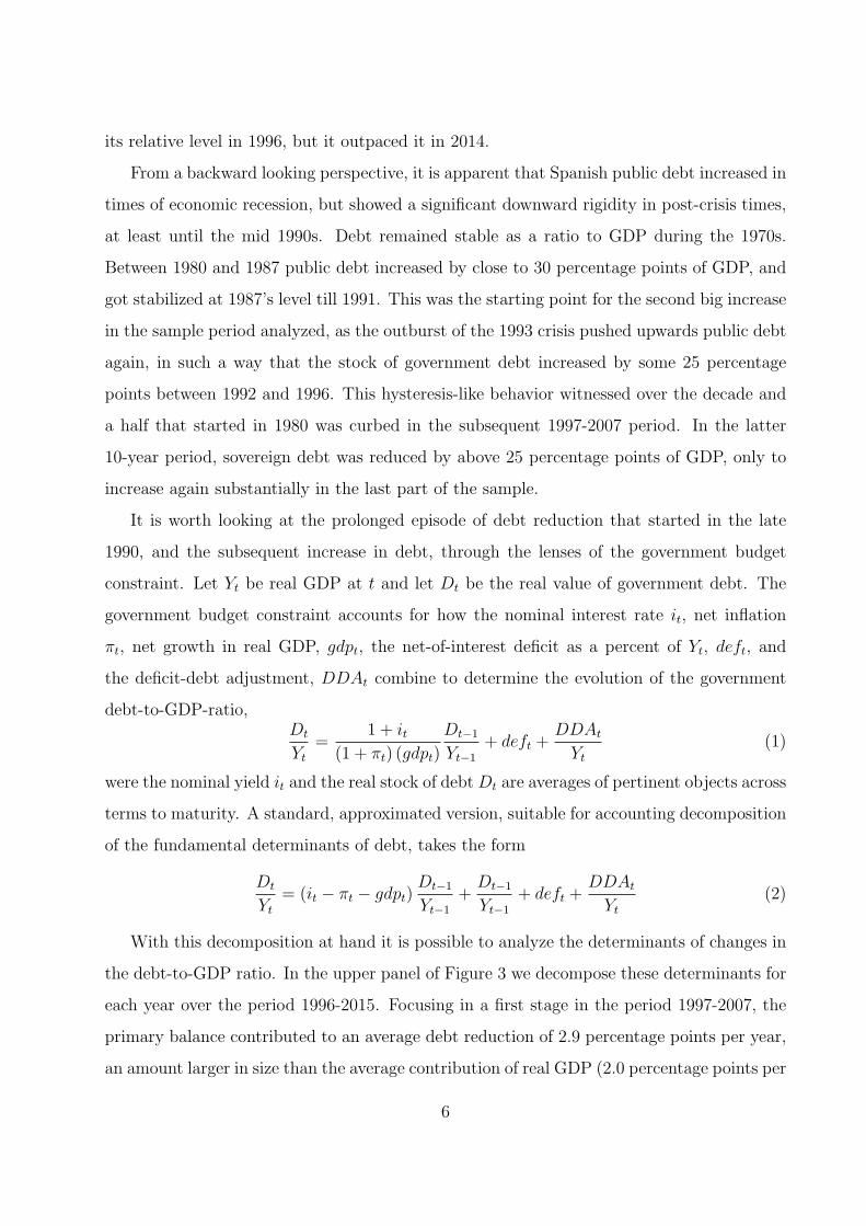
its relative level in 1996, but it outpaced it in 2014.

From a backward looking perspective, it is apparent that Spanish public debt increased in

times of economic recession, but showed a significant downward rigidity in post-crisis times,

at least until the mid 1990s. Debt remained stable as a ratio to GDP during the 1970s.

Between 1980 and 1987 public debt increased by close to 30 percentage points of GDP, and

got stabilized at 1987’s level till 1991. This was the starting point for the second big increase

in the sample period analyzed, as the outburst of the 1993 crisis pushed upwards public debt

again, in such a way that the stock of government debt increased by some 25 percentage

points between 1992 and 1996. This hysteresis-like behavior witnessed over the decade and

a half that started in 1980 was curbed in the subsequent 1997-2007 period. In the latter

10-year period, sovereign debt was reduced by above 25 percentage points of GDP, only to

increase again substantially in the last part of the sample.

It is worth looking at the prolonged episode of debt reduction that started in the late

1990, and the subsequent increase in debt, through the lenses of the government budget

constraint. Let Yt be real GDP at t and let Dt be the real value of government debt. The

government budget constraint accounts for how the nominal interest rate it, net inflation

πt, net growth in real GDP, gdpt, the net-of-interest deficit as a percent of Yt, deft, and

the deficit-debt adjustment, DDAt combine to determine the evolution of the government

debt-to-GDP-ratio,Dt

Yt

=1 + it

(1 + πt) (gdpt)

Dt−1

Yt−1

+ deft +DDAt

Yt

(1)

were the nominal yield it and the real stock of debtDt are averages of pertinent objects across

terms to maturity. A standard, approximated version, suitable for accounting decomposition

of the fundamental determinants of debt, takes the form

Dt

Yt

= (it − πt − gdpt)Dt−1

Yt−1

+Dt−1

Yt−1

+ deft +DDAt

Yt

(2)

With this decomposition at hand it is possible to analyze the determinants of changes in

the debt-to-GDP ratio. In the upper panel of Figure 3 we decompose these determinants for

each year over the period 1996-2015. Focusing in a first stage in the period 1997-2007, the

primary balance contributed to an average debt reduction of 2.9 percentage points per year,

an amount larger in size than the average contribution of real GDP (2.0 percentage points per

6

Figure 3: The determinants of the change in the Spanish public debt-to-GDP ratio.

Year-by-year changes

Cumulative changes

7

year on average) and inflation (1.8 points per year on average). These three positive factors

were partly compensated by an average 0.7 points per year debt-increasing contribution

stemming from deficit-debt adjustments, and the interest payments, that amounted to some

2.9% of GDP per year on average. As regards the 2008-2015 period, the sizeable increase in

debt was basically due to the worsened primary balance (5.3 pp per year), interest payments

(2.5 pp per year), and the adverse contribution of deficit-debt adjustments. To reinforce our

exposition, in the lower panel of Figure 3, in turn, we show the same information as before,

but cumulated, i.e. calculated by means of equation:

Dt

Yt

=τ−1∑s=0

[(it−s − πt−s − gdpt−s)

Dt−s−1

Yt−s−1

+ deft−s +DDAt−s

Yt−s

]+

Dt+τ

Yt+τ

(3)

Between 1996 and 2007, the 26 percentage points of public debt reduction can be broken

down as follows: (i) 35 percentage points of reduction due to the adjustment of the primary

balance; (ii) 23.9 points of reduction due to favorable real GDP growth; (iii) 21.6 percentage

points of reduction due to inflation; (iv) these three factors more than compensated the

increase of 35 points due to the interest payments during the period, and the 7.9 percentage

points due to the deficit-debt adjustments. The debt-increasing contribution of the interest

burden veils a favorable evolution of the implicit interest rate. Interestingly, implicit interest

rate dynamics, that averages interest rates of newly issued debt, including that refinanced,

and rates of non-maturing debt issued in the past, contributed to contain the increase in the

public debt ratio in 2008, 2009 and 2010, only turning to a positive contribution in 2011,

when rates at issuance increased substantially, while displaying a neutral effect in 2012 when

market tensions got substantially reduced. The effect of ECB’s monetary policy measures

on the interest burden of the government becomes clear as of 2012 (see Figure 4). Beyond

this latter factor, in the course of the eight years that span from 2008 to 2015, the abrupt

reversal of all positive factors, most notably the significant primary deficits, undid the results

of the 1997-2007 consolidation period.

After this brief backward-looking description of the contributions of the main determi-

nants of public debt to its evolution, in the subsequent Section we turn to the analysis of

the role of fundamentals in public debt evolution, but from a forward-looking, model-based

point of view.

8

Figure 4: The determinants of the change in the interest payments to GDP ratio

3 Empirical methodology and data

3.1 The data

We use quarterly data from the first quarter of 1986 to the fourth quarter of 2015 of the

following variables: primary deficit over GDP, inflation rate, the implicit interest rate (com-

puted as the ratio between the interest payments in a quarter and the stock of public debt

of the previous period), the growth rate of GDP in real terms and the stock of public debt.

Concerning the spread, the data used covers the period from 1991Q4 to 2015Q4 and it is

computed as the difference between the Spanish 10-year government bond yield and the Ger-

man one, in both cases averaged over the quarter from daily data, taken from Bloomberg.

The data source of the macroeconomic variables in the Spanish National Statistical Institute

(INE), while for the case of fiscal variables, the lack of available official quarterly series leads

us to take the ones from de Castro et al. (2014).

9

3.2 Outline of the methodology

The approach to assess the dynamics and sustainability of public debt is based on the

sequential estimation of a Vector autoregression model, updated each period. As claimed

recently by Polito and Wickens (2011) this is instrumental for the problem at hand in that

it exploits the well-documented advantages of time-series models for forecasting in the short

run (see e.g. Stock and Watson, 2001) and also due to the fact that time-series models tend

to give better forecasts than structural models, particularly in the presence of structural

breaks (see e.g. Clements and Hendry, 2005). Even though we take an agnostic view and

estimate unrestricted VARs (structural models can be written as restricted VARs), we use

the theory to guide our selection of variables. In particular we use the government budget

constraint, as in (1) to select the variables to be included in the analysis.

More in detail, the procedure consists of the following steps. First, given an initial sample

size, a VAR is estimated using the variables that enter into the public debt equation, which in

its simplest form are: the ratio of the primary public deficit over GDP, the nominal interest

rate, the inflation rate and the growth rate of GDP. Second, given the estimated parameters

of the VAR and the corresponding variance-covariance matrix of the errors, a large number

of Monte-Carlo simulations are performed to obtain a large number of realizations of the

innovations and the associated realizations of the macroeconomic fundamentals of the debt

equation. This step entails the computation of the implied debt-to-GDP ratio for different

time horizons depending on the criteria of interest, where the period-by-period government

budget constraint, expressed as a ratio to total GDP takes its non-linear form as in (1).

The procedure can be applied sequentially and allows for the calculation of the proba-

bilistic distribution of the debt ratio for each quarter of the projection. Notice that at each

point in time t the procedure uses the macroeconomic data available up to t − 1 which are

the initial conditions of the relevant variables from which the simulated paths depart, and

consequently the exercise can be used to out-of-sample monitor the evolution of public debt

both in the short and the long term.

10

3.3 VAR model

The first step of the approach entails the sequential estimation of a Vector Autorregression

Model of the following form

Yt = B(L)Yt−1 + Ut. (4)

where

Yt = (gdpt, πt, it, deft) (5)

and Ut is the vector of reduced-form residuals which are assumed to be distributed according

to a multinomial distribution with zero mean and covariance matrix Ω, i.e. Ut ∼ N(0,Ω).

Given the estimated parameters of the VAR and the corresponding variance-covariance ma-

trix of the errors, a large number of Monte-Carlo simulations are performed to obtain a

large number of realizations of the innovations and the associated dynamics of the macroe-

conomic fundamentals. This step entails the computation of the implied debt-to-GDP ratio

for different time horizons depending on the criteria of interest, where the period-by-period

government budget constraint, expressed as a ratio to total GDP is given by equation (1).

3.4 The empirical distribution function of debt levels

The sequential estimation of the VAR and the computation of the simulated paths for public

debt generates, at each point in time, an empirical distribution function of debt levels. This

distribution function, that also depends on the simulation horizon, can be used to monitor

the evolution of public debt in both the short and the long term by computing the corre-

sponding moments of the simulated data. We denote as F Tt (d | It−1) the empirical cumulative

distribution function of debt realizations of length T conditional on the information available

up to period t− 1 (It−1, composed of past data and the estimated parameter coefficients of

the VAR model)

For illustrative purposes Figure 5 displays the cumulative distribution of debt at different

simulation spans (one quarter, one year and two years) when the associated VAR is estimated

with data until 2011Q4 and with data up to 2015Q4. Notice that at short simulation’s

horizons, debt outcomes are distributed tightly around the mean and as the projection

11

Figure 5: Empirical CDF with alternative information sets.

With information up to 2011Q4 With information up to 2015Q4

65 70 75 80 85 90 95 100 105 1100

0.1

0.2

0.3

0.4

0.5

0.6

0.7

0.8

0.9

1

1 quarter1 year2 years

70 80 90 100 110 120 130 1400

0.1

0.2

0.3

0.4

0.5

0.6

0.7

0.8

0.9

1

1 quarter1 year2 years

horizon lengthens, uncertainty increases in such a way that the distribution becomes more fat-

tailed and more extreme outcomes cannot be ruled out. Interestingly, public debt simulations

performed with information up to the end of 2011 anticipated an increase of debt at all

horizons, while for the exercise performed with the sample up to 2015Q4 there is more

heterogeneity, with a non-negligible set of simulated paths indicating a reduction of public

debt.

The distributions generated could be used to perform debt projections starting at the

end of the sample. More generally, in order to assess the forecasting performance of the

procedure in the very short run when compared to the data, Figure 6 displays the average

1-quarter out-of-sample forecast of the macro fundamentals and the public debt over GDP

against the observed data of the corresponding variable. The visual inspection of the graph

indicates that the model correctly approximates the evolution of the main macroeconomic

fundamentals and the public debt in the very short term (1 quarter ahead). The out-of-

sample performance ability of the model to forecast the dynamics of public debt is further

illustrated in Table 1 in which we compare the observed evolution of this item in the data

against the forecast implied by the model at different time horizons. In particular, using the

12

Figure 6: Data (solid lines) versus one-quarter-ahead forecasts (dashed lines).

94Q1 98Q1 02Q1 06Q1 10Q1 14Q1-0.02

-0.01

0

0.01

0.02GDP

EstimatedActual

94Q1 98Q1 02Q1 06Q1 10Q1 14Q1-0.05

0

0.05

0.1

0.15PRIMARY DEFICIT over GDP

94Q1 98Q1 02Q1 06Q1 10Q1 14Q10.005

0.01

0.015

0.02

0.025INTEREST RATE

94Q1 98Q1 02Q1 06Q1 10Q1 14Q130

40

50

60

70

80

90

100PUBLIC DEBT OVER GDP

information available up to the fourth quarter of 2008, we present in panel A the expected

dynamics of public debt in each quarter of 2009 and 2010 implied by the model, while in panel

B we take the fourth quarter of 2010 as forecast origin and display the forecasts for 2011 and

2012, and in panel C the projections with information up to 2013Q4. As mentioned before,

the standard deviation of the forecast increases at longer horizons. Beyond this illustrative

forecast paths, the short-, medium-, and long-term projections of the VARs beat simple

benchmark models like the standard random walk and univariate alternatives to extrapolate

public debt.6

6The results are available from the authors upon request.

13

Table 1: Public debt forecasts at the beginning of the economic crisis (2008Q1), in the midst

of the euro area sovereign debt crisis (2010Q4), and in the recovery phase (2013Q4).

Panel A. Forecast origin 2008Q4.

2009 2010

Q1 Q2 Q3 Q4 Q1 Q2 Q3 Q4

Actual 42.8 46.7 50.5 52.3 55.3 56.5 58.4 59.6

Forecasts: Minimum 38.9 44.6 48.6 52.1 53.1 55.7 56.5 58.2

Forecasts: Mean 40.6 46.3 50.5 54.0 55.2 57.7 58.5 60.5

Forecasts: Maximum 42.4 48.2 52.6 56.2 57.4 60.0 60.6 63.0

Forecast: Standard deviation 0.44 0.49 0.52 0.55 0.57 0.59 0.59 0.61

Panel B. Forecast origin 2010Q4.

2011 2012

Q1 Q2 Q3 Q4 Q1 Q2 Q3 Q4

Actual 62.6 66.5 68.8 69.5 72.4 76.8 79.4 81.4


Forecasts: Mean 61.9 65.1 68.9 71.2 72.1 74.7 79.0 81.2



Panel C. Forecast origin 2013Q4.

2014 2015

Q1 Q2 Q3 Q4 Q1 Q2 Q3 Q4

Actual 95.1 97.5 98.5 98.4 98.4 99.0 98.4 98.3


Forecasts: Mean 95.5 95.7 98.3 99.1 98.9 98.6 98.9 98.4



Note: Excluding deficit-debt adjustments. Public debt figures in each quarter are normalized by nominal GDP in that

quarter, annualized. Thus, the so-computed ratios are different from the standard presentation in which the sum of four

consecutive quarters up to the current one is taken.

14

3.5 The risk measure of public debt and the “prudent” medium-

term level

Apart from the calculation of forecasts, the time dependent empirical distribution function

can also be used to monitor the expected evolution of public debt in probabilistic terms. In

particular, given the distribution function, it is possible to compute the probability of public

debt being higher than a particular threshold θ some quarters ahead T , given the information

available at some point in time denoted as It−1. Notice that the sequence of probabilities will

be time dependent. Formally, at each point in time t the following probability is computed

pTt/t−1(θ) = P (d > θ | It−1) = 1− F Tt (θ | It−1) (6)

and the sequence of such probabilities pTt/t−1(θ) which will be denoted as P Tt/t−1(θ). As

suggested before, one possible way of summarizing the information provided by the time

dependent distribution function of public debt level is to compute the probability of ob-

serving a debt level above some threshold of interest which is deemed to be critical for its

sustainability. An example is the 60% public debt level of reference for the Stability and

Growth Pact and the Spanish Constitution. This exercise, in itself, is useful to monitor

compliance with fiscal rules or simulate alternative scenarios of interest, and as such is used

in the related literature.

In Table 2 we show the correlations of the probability series for a given arbitrarily chosen

threshold (60%) computed for different time spans, and the 10-year bond spread. The

higher correlation is associated with the 10-years horizon, and the probability increases

monotonically as the time horizon approaches that of the spread, showing that there seems

to be some consistency between the time span of the spread (10 years) and the probabilities

computed using the same temporal horizon.

From this point on we move one step forward. One may claim that the probability series

computed taking into account a given threshold should be linked to some market-based

measure of risk in the market for public debt (Garcıa and Rigobon, 2004). In our framework

this is illustrated in Figure 7, were we plot the recursive probability obtained at each point

in time (as measured by the time axis) of breaching the 60% of GDP debt threshold in 10

years from the forecasts origin, i.e. p10yt/t−1(60). Interestingly, just by simple inspection some

15

Table 2: Correlations between the probability and the spread

Time span

1 year 5 years 10 years

1994Q1-2015Q4 0.64 0.59 0.47

1994Q1-2007Q42 0.61 0.51 0.22

1994Q1-2013Q2 0.67 0.62 0.49

close correlation among the two series becomes evident.

Thus, it seems natural to study the linkages between the measure of risk calculated in

(6) and the standard indicator of risk, namely the sovereign bond spread. In this fashion,

we calculate the threshold that maximizes the correlation between our risk measure and

the sovereign bond spread in order to gauge the implicit debt threshold which is the most

consistent with market expectations approximated by the spread. Formally,

θ∗ = argmaxθ

corr(pTt/t−1(θ), St) (7)

i.e. conditional on the information set available at t, It−1, we solve (7) to get the debt

threshold, θ∗, relevant for market participants that use as a reference the time horizon T .

This debt threshold θ∗ can be viewed as the one that shapes market participants expectations

about the evolution of public finances and then as a market based index of debt sustainability.

As such, this does not imply that debt reaches its “maximum affordable” level, as defined

by the fiscal limit (i.e., “...the point beyond which taxes and government expenditures can

no longer adjust to stabilize the value of government debt...”, Leeper and Walker, 2011),

but rather that the debt ratio enters in a region in which the degree of vulnerability of

public finances becomes high, possibly with an associated non-negligible probability of debt

becoming under stress so that the price of bonds drops dramatically to allow for a risk

premium. In that sense, θ∗ is more associated to the lower limit of the probability distribution

of the fiscal limit itself, beyond which the debt ratio displays a small but non negligible

probability of reaching the fiscal limit, thus triggering a non linear response of the spread

(Bi, 2012). In the current circumstance in the euro zone, though, such a response is likely

16

Figure 7: The probability p10yt/t−1(θ) and the sovereign bond spread.

94Q1 96Q3 99Q1 01Q3 04Q1 06Q3 09Q1 11Q3 14Q1

Sov

erei

gn S

prea

d

-100

0

100

200

300

400

500

Pro

babi

lity

0

50

100

spreadprob > 60prob > 90

to be muted by the fact that a major player in the sovereign debt market is present (i.e. the

ECB), as compared to normal periods in which governments are forced to access the market

to cover their financing needs.

4 Some empirical results

The outcome of the implementation of the maximization procedure outlined in the previous

Section to the whole sample until the last quarter of 2015 is displayed in the left panel of

Figure 8, for the case in which we run the simulations with a time span consistent with

the 10-year sovereign spread. There, it is easy to see that the correlation increases until it

reaches a maximum when the debt threshold is 54%, displaying a coefficient of 0.7.

In this context, a natural question that arises is whether the debt threshold has changed

over time, and in particular, to what extent the effects of the crisis has affected the debt

level that is perceived as sustainable by the market. In order to answer this question, we

apply the procedure sequentially starting with a minimum sample size and extending it until

17

Figure 8: The “prudent” public debt threshold

Correlation between the sovereign spread Time variation of the public debt threshold

and the different public debt thresholds that maximizes the correlation with the spread

debt limit20 30 40 50 60 70 80 90 100

corr

elat

ion

0

0.1

0.2

0.3

0.4

0.5

0.6

0.7

0.8

0.9

Quarters00Q2 02Q2 04Q2 06Q2 08Q2 10Q2 12Q2 14Q2

Per

cent

of G

DP

40

42

44

46

48

50

52

54

56

58

60

Public debt threshold

the whole sample is considered, allowing us to study the temporal evolution of the debt

threshold. The results of this latter exercise are shown in in the right panel of Figure 8 and

indicate that the estimated debt threshold has been quite stable in the interval 50% - 55%

of GDP all over the sample since the beginning of the European Monetary Union.

In a final exercise we test whether or not the probability measure Granger-causes the

market risk indicator, St. To do so, we run regressions of the kind:

St = Γ(L) St−1 + Φ(L) pTt/t−1(θ) + ϵt (8)

We show some selected results in Table 3, for the computed probabilities of breaching the

60% limit. The table presents Granger Causality test between St and Pt/t−1, for two different

specifications (lags 4 and 6) and sample size. In addition, we also show in the table the tests

for Pt+1/t. This is warranted as the latter variable is contemporaneous with respect to St

from the point of view of the moment in time in which it is known to the analyst. This is so

because the measure Pt/t−1 is the probability computed for quarter t with data and estimated

parameters up to t− 1, and as a consequence, its information content is lagged with respect

to St. From the results in the table, Pt/t−1 tends to Granger-Causes St, and particularly so

18

Table 3: Granger-causality tests: probability measures and sovereign spread.

4 lags 6 lags

p-values 1994Q1- 1994Q1- 1994Q1- 1994Q1- 1994Q1- 1994Q1-

2015Q4 2013Q4 2007Q4 2015Q4 2013Q4 2007Q4

Pt/t−1 does not Cause St 0.137 0.147 0.129 0.036b 0.074b 0.481

St does not Cause Pt/t−1 0.373 0.361 0.078c 0.816 0.817 0.028a

Pt+1/t does not Cause St 0.006a 0.009a 0.042b 0.003a 0.009a 0.243

St does not Cause Pt+1/t 0.270 0.288 0.000a 0.383 0.274 0.000c

Note: a: null hypothesis rejected at the 1% level, b: 5%, c: 10%.

Pt/t−1 forwarded, for all specifications that incorporate the financial/debt crisis years (i.e.

the null hypothesis of no causation gets rejected). When the 2008-2015 period is excluded,

though, Pt/t−1 does not Granger-cause St: this is a period of debt reduction and strong

fundamentals. Overall, though, the results in Table 3 indicate that the probability measures

contains some real-time, leading indicator value. Compared to St, the measure has the

advantage that is based on macro fundamentals, and thus it might be less affected than St

from episodes of excess volatility or non-fundamental-based reactions by the markets.

5 Conclusions

In this paper we extend previous work that combines the Value at Risk approach with

the estimation of the correlation pattern of the macroeconomic determinants of public debt

dynamics by means of Vector Auto Regressions. These estimated VAR’s are then used to

compute the probability that the public debt ratio exceeds than a given threshold, by means

of Montecarlo simulations.

We apply this methodology to Spanish data and compute time-series probabilities to

analyze the possible correlation with market risk assessment, measured by the spread with

respect to the German bond. Taking into account the high correlation between the prob-

ability of passing a pre-specified debt threshold and the spread, we go a step further and

19

ask what would be the threshold that maximizes the correlation between the two variables.

Thus, by pursuing this approach we are able to gauge the implicit debt threshold or “prudent

debt level” which is consistent with market expectations as measured by the sovereign yield

spread.

References

Aiyagari S. R. and E. R. McGrattan, 1998. The Optimum Quantity of Debt, Journal of

Monetary Economics 42, 447-469.

Aiyagari S. R., A. Marcet, T. J. Sargent and J. Seppala, 2002. Optimal Taxation without

State-Contingent Debt, Journal of Political Economy 110, 1220-1254.

Andres, J. and R. Domenech, 2006. Automatic Stabilizers, Fiscal Rules and Macroeconomic

Stability, European Economic Review 50, pp. 1487-1506.

Bertola G. and A. Drazen, 1993. Trigger Points and Budget Cuts: Explaining the Effects

of Fiscal Austerity, American Economic Review 83, 11-26.

Bi, H., 2012. Sovereign Default Risk Premia, Fiscal Limits and Fiscal Policy, European

Economic Review, 56(3), 389–410.

Bi, H. and E. Leeper, 2013. Analyzing Fiscal Sustainability. Bank of Canada.

Chari V., L. Christiano and P. Kehoe, 1994. Optimal Fiscal Policy in a Business Cycle

Model, Journal of Political Economy 102, 617-652.

Collard, F., M. Habib and J. Rochet, 2014. Sovereign Debt Sustainability in Advanced

Economies. Mimeo.

de Castro, F., F. Marti, A. Montesinos, J. J. Perez, A. J. Sanchez-Fuentes, 2014. Main

stylized facts for the Spanish economy revisited, Bank of Spain Working Paper 1408.

Daniel, C. B. and C. Shiamptanis, 2013. Pushing the limit? Fiscal policy in the European

Monetary Union, Journal of Economic Dynamics and Control, 37, pp. 2307-2321.

20

Delgado-Tellez, M., Gordo, L. and F. Marti, 2016. Developments of public debt in Spain

in 2015, Bank of Spain Economic Bulletin, May.

European Commission, 2011. Public Finances Report (June).

Fall, F. and J.-M. Fournier, 2015. Macroeconomic uncertainties, prudent debt targets and

fiscal rules, OECD Economics Department Working Papers, no 1230.

Floden M., 2001. The effectiveness of government debt and transfers as insurance, Journal

of Monetary Economics 48, 81-108.

Gali, J. and R. Perotti, 2003. Fiscal policy and monetary integration in Europe, Economic

Policy 37, 533-572.

Gosh, A., J. Kim, E. Mendoza, J- Ostry and M. Qureshi, 2015. Fiscal Fatigue, Fiscal Space

and Debt Sustainability in Advanced Economies, The Economic Journal, 123.

Gordo, L., Hernandez de Cos, P. and J. J. Perez, 2013. Developments of public debt in

Spain in 2013. Bank of Spain Economic Bulletin, June-July.

Kleven H.J. and C.T. Kreiner, 2003. The role of taxes as automatic destabilizers in New

Keynesian economics, Journal of Public Economics 87 (2003) 1123—1136.

Leeper, E. M. and T. B. Walker, 2011. Fiscal Limits in Advanced Economies, NBER

Working Papers 16819, National Bureau of Economic Research, Inc.

Melitz J., 2000. Some Cross-Country Evidence about Fiscal Policy Behavior and Conse-

quences for EMU, European Economy 2, 3-21.

Mitchell, P. R., Sault, J. E., and Wallis, K. F., 2000. Fiscal policy rules in macroeconomic

models: Principles and practice. Economic Modelling 17, pp. 171–193.

Polito, V.and M. Wichens, 2011. A model-based indicator of the fiscal stance, European

Economic Review 56, pp. 526-551.

Woodford M., 1990. Public Debt as Private Liquidity, American Economic Review 80,

382-388.

21

Wyplotz C., 1999. Economic Policy Coordination in EMU: Strategies and Institutions.

Mimeo (March).

22

Implicit public debt thresholds: an empirical exercise for the case of ...

Documents

Transcript of Implicit public debt thresholds: an empirical exercise for the case of ...