Implementing the Common Core State Standardswith Precalculus: Graphical, Numerical, Algebraic

Contents

About This Guide .......................................................................................................2 Common Core State Standards For Mathematics............................................................3 Transitioning to the Common Core State Standards ........................................................4 Additional Content for Complete Coverage of the (+) Standards ......................................5

Expanding Section 6.6: Closeness and Betweenness in a Complex World ....................5 Expanding Section 9.3: Random Variables and Expected Value...................................5

The Standards for Mathematical Practices .....................................................................6 Common Core State Standards and Precalculus: Graphical, Numerical, Algebraic, 8th Edition ...............................................................................................11 Closeness and Betweenness in a Complex World ........................................................33 Random Variables and Expected Value.......................................................................37

2

About This Guide

Pearson is pleased to offer this Guide to Implementing the Common Core State Standards as a complement to Precalculus: Graphical, Numerical, Algebraic, 8th edition. In this Guide, you will find information about the Common Core State Standards that can be useful as you look to implement the (+) standards in your precalculus course.

On page 3, you’ll find an overview of the Common Core State Standards, including the recent history leading to their establishment, and a brief description of the Standards for Mathematical Content, with a focus on the (+) standards, and the Standards for Mathematical Practice.

Author Dan Kennedy, Ph.D., contributed his thoughts (pages 4 and 5) on incorporating the Common Core State Standards into this precalculus course. He describes the additional content that has been added and explains why covering the (+) standards will make stronger mathematical thinkers. Kennedy also notes that he and the other authors have embedded in this textbook for many years the practices and habits of mind that the Standards for Mathematical Practice in the Common Core State Standards stress as essential to developing mathematical proficiency (pages 6–10).

Pages 11 through 32 show Correlations of the (+) Standards for Mathematical Content and indicate where the standards are addressed throughout Precalculus: Graphical, Numerical, Algebraic. You’ll notice that in addition to all (+) standards, this course also covers many of the non (+) Standards for Mathematical Content, which are expected to be taught in Algebra 1, Geometry, and Algebra 2.

Beginning on page 33 is the additional content written to ensure complete coverage of (+) standards in the course. Closeness and Betweenness in a Complex World is an extension of Section 6.6 written to inform the student on complex planes. Random Variables and Expected Value expands on Section 9.3 and the textbook’s coverage of probability. Each expanded section is followed by accompanying exercises. Answers to the exercises are on pages 47–49.

3

Common Core State Standards For Mathematics The Common Core State Standards Initiative is a state-led initiative coordinated by the National Governors Association Center for Best Practices (NGA Center) and the Council of Chief State School Officers (CCSSO), with a goal of developing a set of standards in mathematics and in English language arts that would be implemented in many, if not most states in the United States.

The Common Core State Standards for Mathematics (CCSSM) were developed by mathematicians and math educators and reviewed by many professional groups and state department of education representatives of the 48 participating states. The members of the writing committee looked at state standards from high performing states in the United States and from high-performing countries around the world and developed standards that reflect the intent and content of these exemplars.

The final draft was released in June 2010 after nearly 12 months of intense development, review, and revision. To date, over 40 states have adopted these new standards and are

currently working to develop model curricula or curriculum frameworks based on these standards.

These standards identify the knowledge and skills students should gain throughout their K–12 careers so that upon graduation from high school, students will be college- or career-ready. The standards include rigorous content and application of knowledge through higher-order thinking skills.

The CCSSM consist of two interrelated sets of standards, the Standards for Mathematical Practice and the Standards for Mathematical Content. The Standards for Mathematical Practice describe the processes, practices, and dispositions that lead to mathematical proficiency. The eight standards are common to all grade levels, K–12, highlighting that these processes, practices, and dispositions are developed throughout one’s school career. A discussion of these standards is found on pages 6–9. The Standards for Mathematical Content are grade-specific for Kindergarten through Grade 8; at the high school level, the standards are not structured by course or grade; rather they are organized into six conceptual categories. Within each conceptual category are domains and clusters, which each consists of one or more standards. Most of the high school standards are meant to be covered by the end of three years of high school mathematics; a few standards, indicated with (+), represent more advanced topics and expand upon the content learned in the core high school curriculum. These are generally addressed in advanced high school mathematics courses, such as Precalculus, Advanced Statistics, or Discrete Mathematics. An overview of how the (+) standards are addressed in Precalculus: Graphical, Numerical, Algebraic is found on page 5.

These standards identify the knowledge and skills students should gain throughout their K–12 careers so that upon graduation from high school, students will be college- or career-ready.

4

Transitioning to the Common Core State Standards By Daniel Kennedy, Ph.D.

Textbooks like this one evolve in many ways for many reasons, only some of which follow the design of the authors. The primary purpose of a book called precalculus, of course, is to prepare students for courses in calculus, and nine out of ten chapters of our book, Precalculus: Graphical, Numerical, Algberaic, are devoted to doing just that, in what we feel is the most pedagogically effective way. Chapter 9 on Discrete Mathematics, on the other hand, contains quite a bit of material that is not so important for studying calculus, but very important for coping with data in a quantitative world.

In the last few decades, the attention of primary and secondary mathematics education has been shifting slowly but inexorably toward quantitative literacy and away from the classical focus on calculus and its attendant calculations. We have responded by adding more and more material to Chapter 9, all the time wondering whether teachers would have time to cover it in a typical school year. The need to meet every state’s individual standards requirements meant the inclusion of certain precalculus topics, and the exclusion of potentially more useful quantitative literacy material.

That is why the adoption of Common Core State Standards seems to be a fine idea. Once we all agree on what ought to be taught, we can design our textbooks, our teacher development, and our assessments to ensure that students learn that content effectively. (The fact that they could already do this is one of the reasons for the remarkable success of the College Board's Advanced Placement courses over the years.) Eventually, we should be able to design more focused courses at every level and make the textbooks considerably smaller. This will, however, take time.

For now, ironically, most textbooks will actually have to supplement their coverage –– as the country gets serious about quantitative literacy while remaining cautious about curricular reform. We were actually quite pleased that our book was already so consistent with the first set of Common Core State Standards; indeed, we only needed to expand the complex plane coverage in Section 6.6 and the treatment of probability theory in Section 9.3.

5

Additional Content for Complete Coverage of the (+) Standards

Expanding Section 6.6: Closeness and Betweenness in a Complex World

Most precalculus textbooks, ours included, have given scant attention to complex numbers, since they rarely come up in a first-year calculus course. They are algebraically important for understanding the Fundamental Theorem of Algebra, and they tie some important concepts together in DeMoivre's Theorem, but not much knowledge of the complex plane is required for those (primarily algebraic) applications. The Common Core State Standards, obviously looking ahead to courses beyond first-year calculus, have prescribed a somewhat deeper geometrical understanding of the complex plane for college-bound secondary students. This is easily provided with this brief supplement, which could be covered within one class period. As a nice bonus, students will understand why a "complex line" is impossible.

Expanding Section 9.3: Random Variables and Expected Value

From the beginning, one of our strategies for keeping Chapter 9 from becoming too huge was to cover just enough probability theory to explain the statistical applications. (Remember: It's a precalculus book.) This led us to side-step the classical terminology of random variables and expected value, which the Common Core State Standards have now opted to include. Admittedly, it is much easier to explain some statistical concepts (like Bayesian decision-making) if one has access to all that terminology, so it is almost liberating to have it now available through this supplement.

The Common Core vision is that many of the statistical concepts introduced in Chapter 9 will eventually be old news to precalculus students, making the more formal approach to probability theory an appropriate extension at this level. Note that the emphasis is still on the statistical applications, but the probability theory underlying them can be richer.

How long it will take to teach this supplement will be heavily dependent on how much students already know about statistics. In fact, if students are lacking in statistical background, the teacher might want to incorporate examples from Sections 9.7 and 9.8 as needed.

6

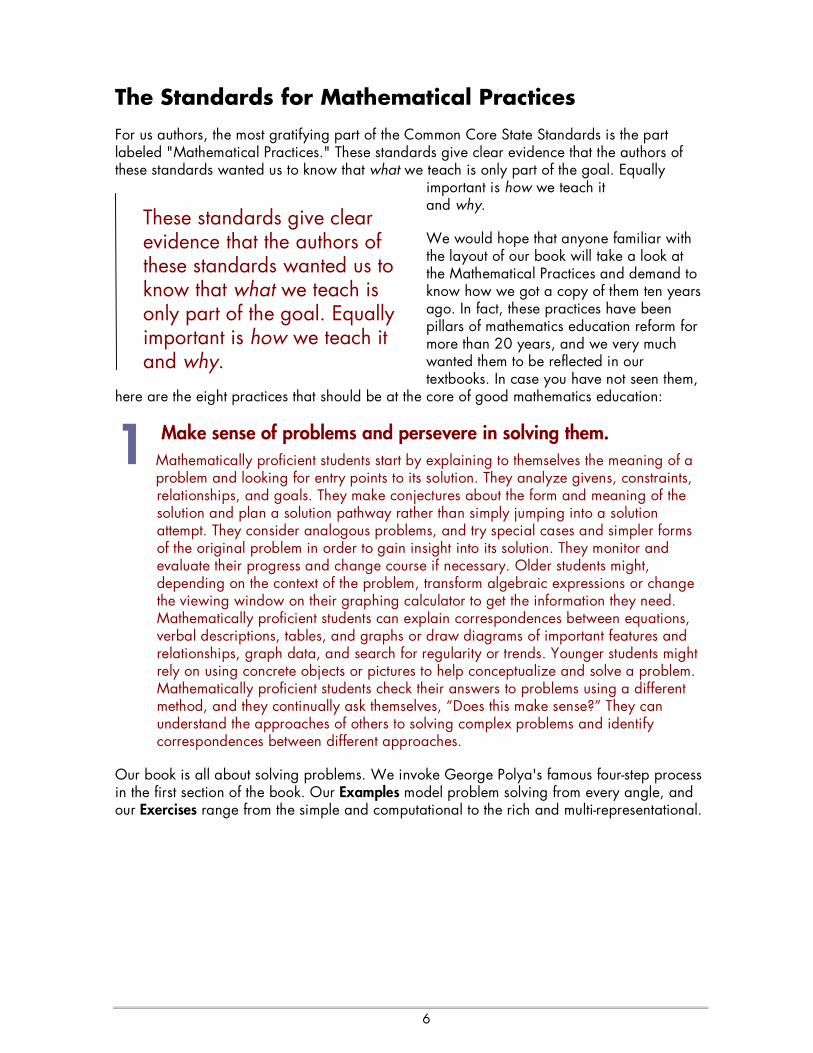
The Standards for Mathematical Practices For us authors, the most gratifying part of the Common Core State Standards is the part labeled "Mathematical Practices." These standards give clear evidence that the authors of these standards wanted us to know that what we teach is only part of the goal. Equally

important is how we teach it and why.

We would hope that anyone familiar with the layout of our book will take a look at the Mathematical Practices and demand to know how we got a copy of them ten years ago. In fact, these practices have been pillars of mathematics education reform for more than 20 years, and we very much wanted them to be reflected in our textbooks. In case you have not seen them,

here are the eight practices that should be at the core of good mathematics education:

Make sense of problems and persevere in solving them. Mathematically proficient students start by explaining to themselves the meaning of a problem and looking for entry points to its solution. They analyze givens, constraints, relationships, and goals. They make conjectures about the form and meaning of the solution and plan a solution pathway rather than simply jumping into a solution attempt. They consider analogous problems, and try special cases and simpler forms of the original problem in order to gain insight into its solution. They monitor and evaluate their progress and change course if necessary. Older students might, depending on the context of the problem, transform algebraic expressions or change the viewing window on their graphing calculator to get the information they need. Mathematically proficient students can explain correspondences between equations, verbal descriptions, tables, and graphs or draw diagrams of important features and relationships, graph data, and search for regularity or trends. Younger students might rely on using concrete objects or pictures to help conceptualize and solve a problem. Mathematically proficient students check their answers to problems using a different method, and they continually ask themselves, “Does this make sense?” They can understand the approaches of others to solving complex problems and identify correspondences between different approaches.

Our book is all about solving problems. We invoke George Polya's famous four-step process in the first section of the book. Our Examples model problem solving from every angle, and our Exercises range from the simple and computational to the rich and multi-representational.

1

These standards give clear evidence that the authors of these standards wanted us to know that what we teach is only part of the goal. Equally important is how we teach it and why.

7

Reason abstractly and quantitatively. Mathematically proficient students make sense of quantities and their relationships in problem situations. They bring two complementary abilities to bear on problems involving quantitative relationships: the ability to decontextualize—to abstract a given situation and represent it symbolically and manipulate the representing symbols as if they have a life of their own, without necessarily attending to their referents—and the ability to contextualize, to pause as needed during the manipulation process in order to probe into the referents for the symbols involved. Quantitative reasoning entails habits of creating a coherent representation of the problem at hand; considering the units involved; attending to the meaning of quantities, not just how to compute them; and knowing and flexibly using different properties of operations and objects.

Ideally, this is what it should mean to "do" mathematics, but many courses get bogged down in quantitative procedures and skills and miss the reasoning part. The Explorations in each section of our book get students to reason things out (abstractly and quantitatively) and thereby discover the procedures. Each set of Exercises includes problems (writing to learn) that reinforce the reasoning step, along with additional explorations and problems designed to extend the ideas.

Construct viable arguments and critique the reasoning of others. Mathematically proficient students understand and use stated assumptions, definitions, and previously established results in constructing arguments. They make conjectures and build a logical progression of statements to explore the truth of their conjectures. They are able to analyze situations by breaking them into cases, and can recognize and use counterexamples. They justify their conclusions, communicate them to others, and respond to the arguments of others. They reason inductively about data, making plausible arguments that take into account the context from which the data arose. Mathematically proficient students are also able to compare the effectiveness of two plausible arguments, distinguish correct logic or reasoning from that which is flawed, and—if there is a flaw in an argument—explain what it is. Elementary students can construct arguments using concrete referents such as objects, drawings, diagrams, and actions. Such arguments can make sense and be correct, even though they are not generalized or made formal until later grades. Later, students learn to determine domains to which an argument applies. Students at all grades can listen or read the arguments of others, decide whether they make sense, and ask useful questions to clarify or improve the arguments.

Although we cannot guarantee that all teachers will use our books as we hope they will, our Explorations are designed to promote this kind of activity in every classroom. Indeed, we hope teachers will use this approach consistently in their teaching so that students will realize that the teacher is not the only one in the classroom who can initiate or sustain a learning experience.

2

3

8

Model with mathematics. Mathematically proficient students can apply the mathematics they know to solve problems arising in everyday life, society, and the workplace. In early grades, this might be as simple as writing an addition equation to describe a situation. In middle grades, a student might apply proportional reasoning to plan a school event or analyze a problem in the community. By high school, a student might use geometry to solve a design problem or use a function to describe how one quantity of interest depends on another. Mathematically proficient students who can apply what they know are comfortable making assumptions and approximations to simplify a complicated situation, realizing that these may need revision later. They are able to identify important quantities in a practical situation and map their relationships using such tools as diagrams, two-way tables, graphs, flowcharts and formulas. They can analyze those relationships mathematically to draw conclusions. They routinely interpret their mathematical results in the context of the situation and reflect on whether the results make sense, possibly improving the model if it has not served its purpose.

This is such an important goal of our book that we have chosen to begin and end our all-important first chapter with sections on modeling. The very name of the book reflects the importance of understanding how to model the real world graphically, numerically, and algebraically. In each new edition of the book we update the numerical data so that students will see how the mathematics they are studying can be used to model the world they are living in right now.

Use appropriate tools strategically. Mathematically proficient students consider the available tools when solving a mathematical problem. These tools might include pencil and paper, concrete models, a ruler, a protractor, a calculator, a spreadsheet, a computer algebra system, a statistical package, or dynamic geometry software. Proficient students are sufficiently familiar with tools appropriate for their grade or course to make sound decisions about when each of these tools might be helpful, recognizing both the insight to be gained and their limitations. For example, mathematically proficient high school students analyze graphs of functions and solutions generated using a graphing calculator. They detect possible errors by strategically using estimation and other mathematical knowledge. When making mathematical models, they know that technology can enable them to visualize the results of varying assumptions, explore consequences, and compare predictions with data. Mathematically proficient students at various grade levels are able to identify relevant external mathematical resources, such as digital content located on a website, and use them to pose or solve problems. They are able to use technological tools to explore and deepen their understanding of concepts.

We doubt that any author team of any precalculus textbook anywhere has been more closely associated with educational technology, particularly graphing calculators, than we have. Not only have we been urging the use of technology in mathematics education for more than two decades, but we have also been vigilant about insisting on the wise use of technology while helpfully pointing out the pitfalls. The strategic use of appropriate tools has been a hallmark of our approach from the start.

4

5

9

Attend to precision. Mathematically proficient students try to communicate precisely to others. They try to use clear definitions in discussion with others and in their own reasoning. They state the meaning of the symbols they choose, including using the equal sign consistently and appropriately. They are careful about specifying units of measure, and labeling axes to clarify the correspondence with quantities in a problem. They calculate accurately and efficiently, express numerical answers with a degree of precision appropriate for the problem context. In the elementary grades, students give carefully formulated explanations to each other. By the time they reach high school they have learned to examine claims and make explicit use of definitions.

We suppose that any mathematical textbook would support this practice philosophically, but we feel strongly enough about it to invest some considerable ink into explaining it to the student. For example, the first section of the book discusses what it means to "solve" a problem and to "prove" that something is true mathematically, and we revisit those ideas in later Examples. It almost goes without saying that we address issues of calculator precision (and the limitations thereof), in context, throughout the book.

Look for and make use of structure. Mathematically proficient students look closely to discern a pattern or structure. Young students, for example, might notice that three and seven more is the same amount as seven and three more, or they may sort a collection of shapes according to how many sides the shapes have. Later, students will see 7 × 8 equals the well remembered 7 × 5 + 7 × 3, in preparation for learning about the distributive property. In the expression x2 + 9x + 14, older students can see the 14 as 2 × 7 and the 9 as 2 + 7. They recognize the significance of an existing line in a geometric figure and can use the strategy of drawing an auxiliary line for solving problems. They also can step back for an overview and shift perspective. They can see complicated things, such as some algebraic expressions, as single objects or as being composed of several objects. For example, they can see 5 – 3(x – y)2 as 5 minus a positive number times a square and use that to realize that its value cannot be more than 5 for any real numbers x and y.

We essentially used this practice as our guiding principle when reworking the order of topics in this book. Graphing calculators enabled us to expose students to the comparative study of functions before becoming immersed in their algebraic behavior, so we did. Students could thereby appreciate (and hopefully discuss) the structure of functions from the beginning of the course, thus raising to a new level the unifying principle of function first envisioned by Leonhard Euler in 1748. It is also a guiding principle of our book that students will understand function behavior in all its representations: graphical, numerical, algebraic, and verbal.

6

7

10

Look for and express regularity in repeated reasoning. Mathematically proficient students notice if calculations are repeated, and look both for general methods and for shortcuts. Upper elementary students might notice when dividing 25 by 11 that they are repeating the same calculations over and over again, and conclude they have a repeating decimal. By paying attention to the calculation of slope as they repeatedly check whether points are on the line through (1, 2) with slope 3, middle school students might abstract the equation (y – 2)/(x – 1) = 3. Noticing the regularity in the way terms cancel when expanding (x – 1)(x + 1), (x – 1)(x2 + x + 1), and (x – 1)(x3 + x2 + x + 1) might lead them to the general formula for the sum of a geometric series. As they work to solve a problem, mathematically proficient students maintain oversight of the process, while attending to the details. They continually evaluate the reasonableness of their intermediate results.

Every Example in our textbook is paired with an Exercise that allows students to affirm their understanding by employing this mathematical practice. Constructive learning is ideal when it works, but students can also learn by seeing examples, then looking for and expressing regularity by solving similar problems. This is also how homework plays a role, and we have much to say about homework in our book, including when calculator use is appropriate and when it is not.

We hope that all of these Mathematical Practices will resonate strongly with teachers who have been using Precalculus: Graphical, Numerical, Algebraic. The more we can incorporate them into our daily teaching, the better it will be for our students. We expect some adjustments to be made to the Common Core State Standards in the near future regarding what topics should realistically be taught and when, but in our estimation the how and the why seem to be on pretty firm ground already.

8

11

Common Core State Standards Precalculus: Graphical, Numerical, Algebraic, 8th Edition

The following shows the alignment of Precalculus, Graphical, Numerical, Algebraic to the High School Standards for Mathematical Content in the Common Core State Standards. We have included all of the standards, both non (+) and (+), to help teachers understand the progression of concepts and skills in high school mathematics. However, the goal of Precalculus: Graphical, Numerical, Algebraic is to cover only those standards marked in red with a (+). You'll notice there are coverage gaps in some of the non (+) standards as they are meant to be studied before taking this course.

Key N-RN.1 non (+) standards that students study in Algebra 1, Geometry, and Algebra 2

N-CN.3 (+) (+) standards, the main focus of study in fourth-year courses, like precalculus

★ modeling standards

TE page references in the annotated Teacher’s Edition

TK page references in the additional lessons of this Transition Kit

‘See related concepts and

skills.’

indicates there is no direct instruction, but there is a lesson(s) that can be used to create instruction

You'll notice Geometry (+) standard G.GMD.2, which requires informal arguments using Cavelieri’s principle with respect to formulas for volume of a sphere and other solid figures, is not covered in this course. The authors believe formulas for volume should be taught in geometry courses and therefore this standard is covered in Pearson’s Geometry text.

Number and Quantity

The Real Number System N-RN

Extend the properties of exponents to rational exponents.

N-RN.1 Explain how the definition of the meaning of rational exponents follows from extending the properties of integer exponents to those values, allowing for a notation for radicals in terms of rational exponents.

TE: 7, 781–783

N-RN.2 Rewrite expressions involving radicals and rational exponents using the properties of exponents.

TE: 780–783

Use properties of rational and irrational numbers.

N-RN.3 Explain why the sum or product of two rational numbers is rational; that the sum of a rational number and an irrational number is irrational; and that the product of a nonzero rational number and an irrational number is irrational.

See related concepts and skills. TE: 2

12

Quantities N-Q

Reason quantitatively and use units to solve problems.

N-Q.1 Use units as a way to understand problems and to guide the solution of multi-step problems; choose and interpret units consistently in formulas; choose and interpret the scale and the origin in graphs and data displays.

TE: 66–67, 76 (#25–#28), 107 (#56), 126 (#34), 183 (#53), 193–194(#66–#68), 233 (#31), 263 (#58), 318, 397 (#36), 402, 517, 640, 733

N-Q.2 Define appropriate quantities for the purpose of descriptive modeling.

TE: 250, 318, 402, 517, 640, 733

N-Q.3 Choose a level of accuracy appropriate to limitations on measurement when reporting quantities.

TE: 250, 318, 402, 517, 640, 733

The Complex Number System N-CN

Perform arithmetic operations with complex numbers.

N-CN.1 Know there is a complex number i such that i2 = –1, and every complex number has the form a + bi with a and b real.

TE: 49

N-CN.2 Use the relation i2 = –1 and the commutative, associative, and distributive properties to add, subtract, and multiply complex numbers.

TE: 49–50, 51, 52, 53, 62, 505–506, 511

N-CN.3 (+) Find the conjugate of a complex number; use conjugates to find moduli and quotients of complex numbers.

TE: 51, 53 (#33–#40), 62 (#80), 504–506, 511

Represent complex numbers and their operations on the complex plane.

N-CN.4 (+) Represent complex numbers on the complex plane in rectangular and polar form (including real and imaginary numbers), and explain why the rectangular and polar forms of a given complex number represent the same number.

TE: 503–505, 511, 515

N-CN.5 (+) Represent addition, subtraction, multiplication, and conjugation of complex numbers geometrically on the complex plane; use properties of this representation for computation.

TE: 49, 50, 51, 52, 53, 62, 505, 506, 511, 515

N-CN.6 (+) Calculate the distance between numbers in the complex plane as the modulus of the difference, and the midpoint of a segment as the average of the numbers at its endpoints.

TK: 6.6.1 Also see related concepts and skills. TE: 49, 52, 503, 504, 511

13

Use complex numbers in polynomial identities and equations.

N-CN.7 Solve quadratic equations with real coefficients that have complex solutions.

TE: 213, 215 (#27–#36), 247 (#49–#52)

N-CN.8 (+) Extend polynomial identities to the complex numbers. TE: 49–51

N-CN.9 (+) Know the Fundamental Theorem of Algebra; show that it is true for quadratic polynomials.

TE: 210, 211 215 (#21)

Vector and Matrix Quantities N-VM

Represent and model with vector quantities.

N-VM.1 (+) Recognize vector quantities as having both magnitude and direction. Represent vector quantities by directed line segments, and use appropriate symbols for vectors and their magnitudes (e.g., v, |v|, ||v||, v).

TE: 456–458, 633

N-VM.2 (+) Find the components of a vector by subtracting the coordinates of an initial point from the coordinates of a terminal point.

TE: 456, 461, 464 (#29–#32)

N-VM.3 (+) Solve problems involving velocity and other quantities that can be represented by vectors.

TE: 461–463, 465, 515 (#74, #75), 516 (#76, #77)

Perform operations on vectors.

N-VM.4.a Add vectors end-to-end, component-wise, and by the parallelogram rule. Understand that the magnitude of a sum of two vectors is typically not the sum of the magnitudes. b. Given two vectors in magnitude and direction form, determine the magnitude and direction of their sum.

TE: 458–459, 464 (#13, #14)

N-VM.4.b Given two vectors in magnitude and direction form, determine the magnitude and direction of their sum.

TE: 460–462, 465 (#49, #50)

N-VM.4 (+) Add and subtract vectors.

N-VM.4.c Understand vector subtraction v – w as v + (–w), where –w is the additive inverse of w, with the same magnitude as w and pointing in the opposite direction. Represent vector subtraction graphically by connecting the tips in the appropriate order, and perform vector subtraction component-wise.

TE: 464 (#15, #18–#20), 514 (#1, #2)

14

N-VM.5.a Represent scalar multiplication graphically by scaling vectors and possibly reversing their direction; perform scalar multiplication component-wise, e.g., as c(vx, vy) = (cvx, cvy).

TE: 459, 464 (#16)

N-VM.5 (+) Multiply a vector by a scalar.

N-VM.5.b Compute the magnitude of a scalar multiple cv using ||cv|| = |c|v. Compute the direction of cv knowing that when |c|v ≠ 0, the direction of cv is either along v (for c > 0) or against v (for c < 0).

TE: 458–459

Perform operations on matrices and use matrices in applications.

N-VM.6 (+) Use matrices to represent and manipulate data, e.g., to represent payoffs or incidence relationships in a network.

TE: 531, 533–534, 541

N-VM.7 (+) Multiply matrices by scalars to produce new matrices, e.g., as when all of the payoffs in a game are doubled.

TE: 531, 540 (#11c–#16c), 573 (#1c, #2c)

N-VM.8 (+) Add, subtract, and multiply matrices of appropriate dimensions.

TE: 530–534, 540 (#11–#28), 573 (#1–#8)

N-VM.9 (+) Understand that, unlike multiplication of numbers, matrix multiplication for square matrices is not a commutative operation, but still satisfies the associative and distributive properties.

TE: 537

N-VM.10 (+) Understand that the zero and identity matrices play a role in matrix addition and multiplication similar to the role of 0 and 1 in the real numbers. The determinant of a square matrix is nonzero if and only if the matrix has a multiplicative inverse.

TE: 532, 534–535, 537, 540, 541

N-VM.11 (+) Multiply a vector (regarded as a matrix with one column) by a matrix of suitable dimensions to produce another vector. Work with matrices as transformations of vectors.

See related concepts and skills. TE: 532, 540 (#15, #16, #23, #24)

N-VM.12 (+) Work with 2 × 2 matrices as transformations of the plane, and interpret the absolute value of the determinant in terms of area.

See related concepts and skills. TE: 535, 537–538

15

Algebra

Seeing Structure in Expressions A-SSE

Interpret the structure of expressions

A-SSE.1.a Interpret parts of an expression, such as terms, factors, and coefficients.

TE: 779–783, 784–790, 791–795

A-SSE.1 Interpret expressions that represent a quantity in terms of its context.★

A-SSE.1.b Interpret complicated expressions by viewing one or more of their parts as a single entity.

TE: 785–790

A-SSE.2 Use the structure of an expression to identify ways to rewrite it.

TE: 780–783, 784–790, 791–795

Write expressions in equivalent forms to solve problems

A-SSE.3.a Factor a quadratic expression to reveal the zeros of the function it defines.

TE: 40, 46 (#1–#6), 785–786, 789

A-SSE.3.b Complete the square in a quadratic expression to reveal the maximum or minimum value of the function it defines.

TE: 41–42, 46 (#13–#18), 166, 169 (#33–#38)

A-SSE.3 Choose and produce an equivalent form of an expression to reveal and explain properties of the quantity represented by the expression.★

A-SSE.3.c Use the properties of exponents to transform expressions for exponential functions.

TE: 270, 305, 306, 310

A-SSE.4 Derive the formula for the sum of a finite geometric series (when the common ratio is not 1), and use the formula to solve problems.★

TE: 680–681, 685 (#37, #38), 731 (#75, #76)

Arithmetic with Polynomials and Rational Expressions A-APR

Perform arithmetic operations on polynomials

A-APR.1 Understand that polynomials form a system analogous to the integers, namely, they are closed under the operations of addition, subtraction, and multiplication; add, subtract, and multiply polynomials.

TE: 784–785, 789 (#9–#18)

Understand the relationship between zeros and factors of polynomials

A-APR.2 Know and apply the Remainder Theorem: For a polynomial p(x) and a number a, the remainder on division by x – a is p(a), so p(a) = 0 if and only if (x – a) is a factor of p(x).

TE: 198–199, 204 (#13–#18), 246 (#29, #30)

16

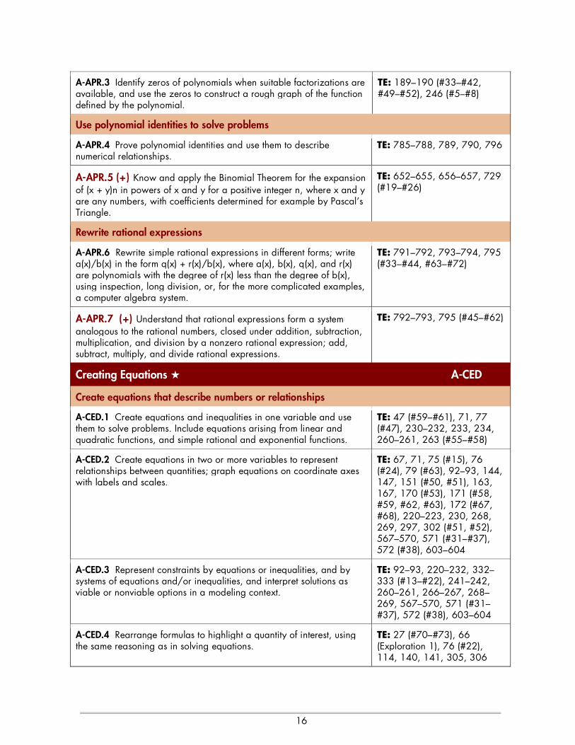
A-APR.3 Identify zeros of polynomials when suitable factorizations are available, and use the zeros to construct a rough graph of the function defined by the polynomial.

TE: 189–190 (#33–#42, #49–#52), 246 (#5–#8)

Use polynomial identities to solve problems

A-APR.4 Prove polynomial identities and use them to describe numerical relationships.

TE: 785–788, 789, 790, 796

A-APR.5 (+ ) Know and apply the Binomial Theorem for the expansion of (x + y)n in powers of x and y for a positive integer n, where x and y are any numbers, with coefficients determined for example by Pascal’s Triangle.

TE: 652–655, 656–657, 729 (#19–#26)

Rewrite rational expressions

A-APR.6 Rewrite simple rational expressions in different forms; write a(x)/b(x) in the form q(x) + r(x)/b(x), where a(x), b(x), q(x), and r(x) are polynomials with the degree of r(x) less than the degree of b(x), using inspection, long division, or, for the more complicated examples, a computer algebra system.

TE: 791–792, 793–794, 795 (#33–#44, #63–#72)

A-APR.7 (+) Understand that rational expressions form a system analogous to the rational numbers, closed under addition, subtraction, multiplication, and division by a nonzero rational expression; add, subtract, multiply, and divide rational expressions.

TE: 792–793, 795 (#45–#62)

Creating Equations ★ A-CED

Create equations that describe numbers or relationships

A-CED.1 Create equations and inequalities in one variable and use them to solve problems. Include equations arising from linear and quadratic functions, and simple rational and exponential functions.

TE: 47 (#59–#61), 71, 77 (#47), 230–232, 233, 234, 260–261, 263 (#55–#58)

A-CED.2 Create equations in two or more variables to represent relationships between quantities; graph equations on coordinate axes with labels and scales.

TE: 67, 71, 75 (#15), 76 (#24), 79 (#63), 92–93, 144, 147, 151 (#50, #51), 163, 167, 170 (#53), 171 (#58, #59, #62, #63), 172 (#67, #68), 220–223, 230, 268, 269, 297, 302 (#51, #52), 567–570, 571 (#31–#37), 572 (#38), 603–604

A-CED.3 Represent constraints by equations or inequalities, and by systems of equations and/or inequalities, and interpret solutions as viable or nonviable options in a modeling context.

TE: 92–93, 220–232, 332–333 (#13–#22), 241–242, 260–261, 266–267, 268–269, 567–570, 571 (#31–#37), 572 (#38), 603–604

A-CED.4 Rearrange formulas to highlight a quantity of interest, using the same reasoning as in solving equations.

TE: 27 (#70–#73), 66 (Exploration 1), 76 (#22), 114, 140, 141, 305, 306

17

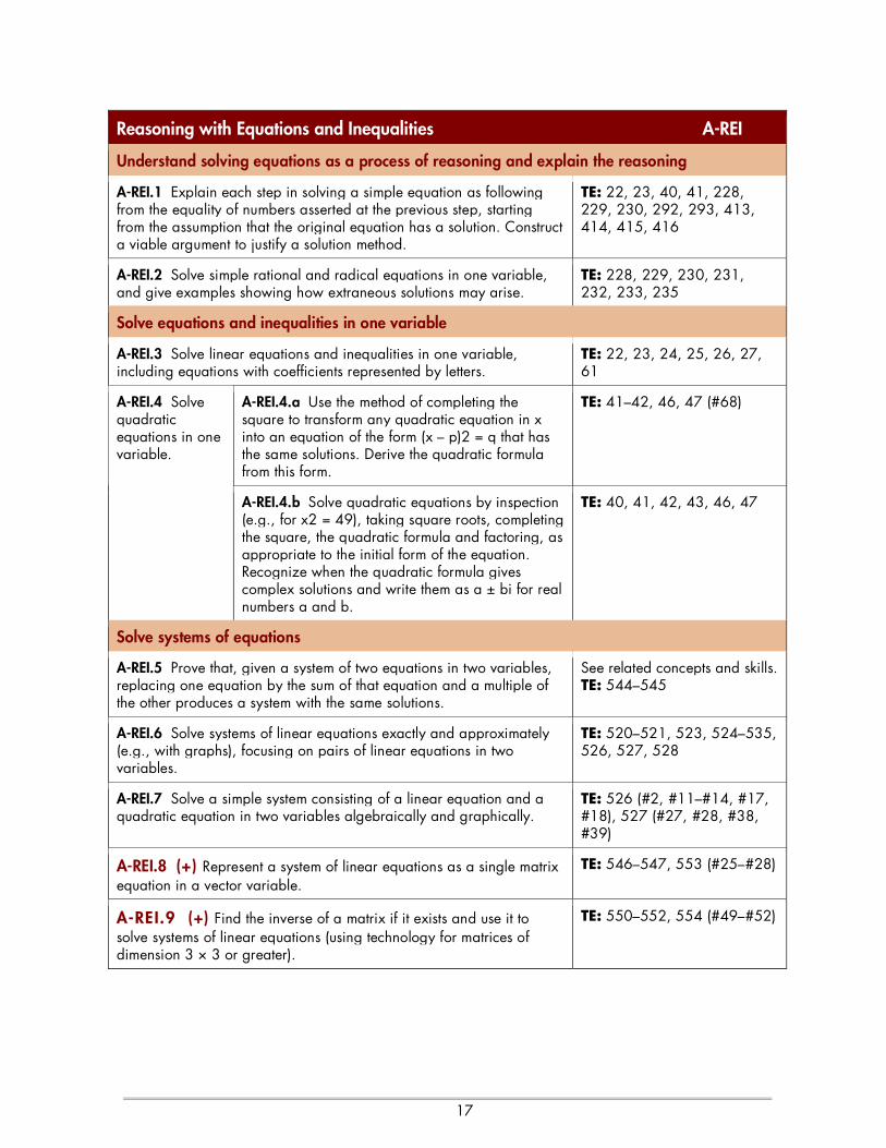
Reasoning with Equations and Inequalities A-REI

Understand solving equations as a process of reasoning and explain the reasoning

A-REI.1 Explain each step in solving a simple equation as following from the equality of numbers asserted at the previous step, starting from the assumption that the original equation has a solution. Construct a viable argument to justify a solution method.

TE: 22, 23, 40, 41, 228, 229, 230, 292, 293, 413, 414, 415, 416

A-REI.2 Solve simple rational and radical equations in one variable, and give examples showing how extraneous solutions may arise.

TE: 228, 229, 230, 231, 232, 233, 235

Solve equations and inequalities in one variable

A-REI.3 Solve linear equations and inequalities in one variable, including equations with coefficients represented by letters.

TE: 22, 23, 24, 25, 26, 27, 61

A-REI.4.a Use the method of completing the square to transform any quadratic equation in x into an equation of the form (x – p)2 = q that has the same solutions. Derive the quadratic formula from this form.

TE: 41–42, 46, 47 (#68)

A-REI.4 Solve quadratic equations in one variable.

A-REI.4.b Solve quadratic equations by inspection (e.g., for x2 = 49), taking square roots, completing the square, the quadratic formula and factoring, as appropriate to the initial form of the equation. Recognize when the quadratic formula gives complex solutions and write them as a ± bi for real numbers a and b.

TE: 40, 41, 42, 43, 46, 47

Solve systems of equations

A-REI.5 Prove that, given a system of two equations in two variables, replacing one equation by the sum of that equation and a multiple of the other produces a system with the same solutions.

See related concepts and skills. TE: 544–545

A-REI.6 Solve systems of linear equations exactly and approximately (e.g., with graphs), focusing on pairs of linear equations in two variables.

TE: 520–521, 523, 524–535, 526, 527, 528

A-REI.7 Solve a simple system consisting of a linear equation and a quadratic equation in two variables algebraically and graphically.

TE: 526 (#2, #11–#14, #17, #18), 527 (#27, #28, #38, #39)

A-REI.8 (+ ) Represent a system of linear equations as a single matrix equation in a vector variable.

TE: 546–547, 553 (#25–#28)

A-REI.9 (+) Find the inverse of a matrix if it exists and use it to solve systems of linear equations (using technology for matrices of dimension 3 × 3 or greater).

TE: 550–552, 554 (#49–#52)

18

Represent and solve equations and inequalities graphically

A-REI.10 Understand that the graph of an equation in two variables is the set of all its solutions plotted in the coordinate plane, often forming a curve (which could be a line).

TE: 31, 36 (#27–#30), #37 (#51, #52), 69, 83, 87–88, 89, 91–92, 93–94, 95 (#21–#24, #29–#34), 96 (#63–#66), 99–101, 105, 106 (#1–#12), 107 (#53–#56), 108 (#64), 164–165, 169, (#13–#18), 176–179, 182 (#37–#42), 185, 193 (#9–#12), 219–220, 225 (#5–#10), 226 (#31–#36), 255, 256, 258, 259, 262 (#15–#30), 278, 279, 281 (#37–#58), 350, 351, 357 (#13–#28), 361–362, 363–364, 365 (#1–#12), 366 (#13–#16)

A-REI.11 Explain why the x-coordinates of the points where the graphs of the equations y = f(x) and y = g(x) intersect are the solutions of the equation f(x) = g(x); find the solutions approximately, e.g., using technology to graph the functions, make tables of values, or find successive approximations. Include cases where f(x) and/or g(x) are linear, polynomial, rational, absolute value, exponential, and logarithmic functions.★

TE: 520–522, 523, 524, 525, 526 (#13–#18), 527 (#35–#42), 529 (#65, #66)

A-REI.12 Graph the solutions to a linear inequality in two variables as a halfplane (excluding the boundary in the case of a strict inequality), and graph the solution set to a system of linear inequalities in two variables as the intersection of the corresponding half-planes.

TE: 565–566, 567 570, 571, 574, 575

19

Functions

Interpreting Functions F-IF

Understand the concept of a function and use function notation

F-IF.1 Understand that a function from one set (called the domain) to another set (called the range) assigns to each element of the domain exactly one element of the range. If f is a function and x is an element of its domain, then f(x) denotes the output of f corresponding to the input x. The graph of f is the graph of the equation y = f(x).

TE: 80–84, 94, 95, 96, 97, 99–105, 106, 107, 152, 153

F-IF.2 Use function notation, evaluate functions for inputs in their domains, and interpret statements that use function notation in terms of a context.

TE: 83–84. 95 (#9–#16, #17–#20), 97 (#78), 107 (#56), 140–147, 148 (#15–#20), 150 (#49), 153 (#11–#18), 154 (#59–#64)

F-IF.3 Recognize that sequences are functions, sometimes defined recursively, whose domain is a subset of the integers.

TE: 670–675, 676, 677, 730 (#47–#62)

Interpret functions that arise in applications in terms of the context

F-IF.4 For a function that models a relationship between two quantities, interpret key features of graphs and tables in terms of the quantities, and sketch graphs showing key features given a verbal description of the relationship. Key features include: intercepts; intervals where the function is increasing, decreasing, positive, or negative; relative maximums and minimums; symmetries; end behavior; and periodicity.★

TE: 159–163, 164–168, 170, 171, 172, 176–181, 183, 184, 185–192, 194, 195, 218–224, 227, 248, 249, 250, 252–261, 262, 263, 265–270, 271, 272, 273, 277–280, 281, 282, 290, 291, 350–356, 358, 359, 360, 361–364, 367

F-IF.5 Relate the domain of a function to its graph and, where applicable, to the quantitative relationship it describes.★

TE: 81–82, 95, 99–102, 105, 106, 140–141, 176–181, 219, 224, 255, 259, 266, 267, 268, 269, 270, 278, 350, 356, 361, 362, 363, 364

F-IF.6 Calculate and interpret the average rate of change of a function (presented symbolically or as a table) over a specified interval. Estimate the rate of change from a graph.★

TE: 160–161, 170 (#53), 171 (60), 172 (#67), 173 (#78)

20

Analyze functions using different representations

F-IF.7.a Graph linear and quadratic functions and show intercepts, maxima, and minima.

TE: 66–68, 99, 103–104, 106, 159–163, 164–168, 169, 170, 171, 172, 173, 246, 247, 248, 249, 250

F-IF.7.b Graph square root, cube root, and piecewise-defined functions, including step functions and absolute value functions.

TE: 100, 101, 103, 104–105, 106, 107, 108, 179

F-IF.7.c Graph polynomial functions, identifying zeros when suitable factorizations are available, and showing end behavior.

TE: 158–168, 169, 170, 171, 172, 173, 185–192, 193, 194, 195, 196, 246, 247, 248, 249, 250

F-IF.7.d (+) Graph rational functions, identifying zeros and asymptotes when suitable factorizations are available, and showing end behavior.

TE: 218–224, 225, 226, 227, 247

F-IF.7 Graph functions expressed symbolically and show key features of the graph, by hand in simple cases and using technology for more complicated cases.★

F-IF.7.e Graph exponential and logarithmic functions, showing intercepts and end behavior, and trigonometric functions, showing period, midline, and amplitude.

TE: 252–258, 260, 262, 266–268, 274, 277–279, 281, 314, 315, 318

F-IF.8.a Use the process of factoring and completing the square in a quadratic function to show zeros, extreme values, and symmetry of the graph, and interpret these in terms of a context.

TE: 40–43, 47 (#1–#6, #13–#18), 145, 164–168, 169, 171 (#61–#65), 246, 248, 249, 250

F-IF.8 Write a function defined by an expression in different but equivalent forms to reveal and explain different properties of the function.

F-IF.8.b Use the properties of exponents to interpret expressions for exponential functions.

TE: 7, 253, 254, 260, 262 (#39, #40), 265–267, 270 (#1–#6), 271 (#29–#34), 272, 273

F-IF.9 Compare properties of two functions each represented in a different way (algebraically, graphically, numerically in tables, or by verbal descriptions).

TE: 90–92, 103–104, 105, 176, 179, 219, 255, 256, 259, 350, 351, 361, 362, 363, 364

21

Building Functions F-BF

Build a function that models a relationship between two quantities

F-BF.1.a Determine an explicit expression, a recursive process, or steps for calculation from a context.

TE: 254, 261 (#11, #12), 266, 267, 271 (#58, #59, #62, #63), 191, 248 (#83, #85, #86), 249 (#90, #93–#95), 395 (#27, #28), 396 (#29, #32), 670–671, 672–673, 674–675, 676 (#1–#10, #21–#31),

F-BF.1.b Combine standard function types using arithmetic operations.

TE: 110, 116 (#1–#8), 117 (#9, #10)

F-BF.1 Write a function that describes a relationship between two quantities.★

F-BF.1.c (+) Compose functions. TE: 111–114, 117, 118, 154

F-BF.2 Write arithmetic and geometric sequences both recursively and with an explicit formula, use them to model situations, and translate between the two forms.★

TE: 670–675, 676, 677

Build new functions from existing functions

F-BF.3 Identify the effect on the graph of replacing f(x) by f(x) + k, k f(x), f(kx), and f(x + k) for specific values of k (both positive and negative); find the value of k given the graphs. Experiment with cases and illustrate an explanation of the effects on the graph using technology. Include recognizing even and odd functions from their graphs and algebraic expressions for them.

TE: 90–92, 95 (#47–#54), 103–104, 105, 129–136, 137, 138, 139, 153 (#37–#40), 176, 179, 185, 219, 220, 255, 256, 258, 259, 350, 351, 352, 353, 355, 361

F-BF.4.a Solve an equation of the form f(x) = c for a simple function f that has an inverse and write an expression for the inverse.

TE: 121–125, 126, 127, 128

F-BF.4.b (+) Verify by composition that one function is the inverse of another.

TE: 124, 129 (#27–#32)

F-BF.4.c (+) Read values of an inverse function from a graph or a table, given that the function has an inverse.

TE: 123–124, 126 (#23–#26)

F-BF.4 Find inverse functions.

F-BF.4.d (+) Produce an invertible function from a non-invertible function by restricting the domain.

TE: 123–124, 126 (#23–#26)

F-BF.5 (+ ) Understand the inverse relationship between exponents and logarithms and use this relationship to solve problems involving logarithms and exponents.

TE: 274–277, 281, 283, 285, 288, 293, 297, 298

22

Linear, Quadratic, and Exponential Models★ F-LE

Construct and compare linear, quadratic, and exponential models and solve problems

F-LE.1.a Prove that linear functions grow by equal differences over equal intervals, and that exponential functions grow by equal factors over equal intervals.

See related concepts and skills. TE: 33 (Figure P.29(b)), 160–161, 170 (#51, #52), 254–255, 261 (#11, #12)

F-LE.1.b Recognize situations in which one quantity changes at a constant rate per unit interval relative to another.

TE: 160–163, 170 (#53), 172 (#67, #68)

F-LE.1 Distinguish between situations that can be modeled with linear functions and with exponential functions. F-LE.1.c Recognize situations in which a quantity

grows or decays by a constant percent rate per unit interval relative to another.

TE: 260–261, 262 (#51), 263 (#52–#58), 265–270, 271, 272, 273

F-LE.2 Construct linear and exponential functions, including arithmetic and geometric sequences, given a graph, a description of a relationship, or two input-output pairs (include reading these from a table).

TE: 33–34, 37 (#45, #51), 163, 170 (#53), 172 (#67, #68), 266–268, 271 (#33, #34), 272

F-LE.3 Observe using graphs and tables that a quantity increasing exponentially eventually exceeds a quantity increasing linearly, quadratically, or (more generally) as a polynomial function.

TE: 258–261, 262 (#51–#56)

F-LE.4 For exponential models, express as a logarithm the solution to abct = d where a, c, and d are numbers and the base b is 2, 10, or e; evaluate the logarithm using technology.

TE: 296–297 (Example 7), 301 (#49, #50)

Interpret expressions for functions in terms of the situation they model

F-LE.5 Interpret the parameters in a linear or exponential function in terms of a context.

TE: 258–261, 263 (#56), 269–270, 272 (#46), 273 (#58), 316 (#76, #94)

23

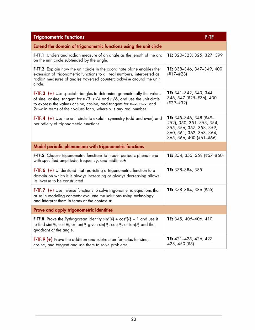
Trigonometric Functions F-TF

Extend the domain of trigonometric functions using the unit circle

F-TF.1 Understand radian measure of an angle as the length of the arc on the unit circle subtended by the angle.

TE: 320–323, 325, 327, 399

F-TF.2 Explain how the unit circle in the coordinate plane enables the extension of trigonometric functions to all real numbers, interpreted as radian measures of angles traversed counterclockwise around the unit circle.

TE: 338–346, 347–349, 400 (#17–#28)

F-TF.3 (+) Use special triangles to determine geometrically the values of sine, cosine, tangent for π/3, π/4 and π/6, and use the unit circle to express the values of sine, cosine, and tangent for π–x, π+x, and 2π–x in terms of their values for x, where x is any real number.

TE: 341–342, 343, 344, 346, 347 (#25–#36), 400 (#29–#32)

F-TF.4 (+) Use the unit circle to explain symmetry (odd and even) and periodicity of trigonometric functions.

TE: 345–346, 348 (#49–#52), 350, 351, 353, 354, 355, 356, 357, 358, 359, 360, 361, 362, 363, 364, 365, 366, 400 (#61–#66)

Model periodic phenomena with trigonometric functions

F-TF.5 Choose trigonometric functions to model periodic phenomena with specified amplitude, frequency, and midline.★

TE: 354, 355, 358 (#57–#60)

F-TF.6 (+) Understand that restricting a trigonometric function to a domain on which it is always increasing or always decreasing allows its inverse to be constructed.

TE: 378–384, 385

F-TF.7 (+) Use inverse functions to solve trigonometric equations that arise in modeling contexts; evaluate the solutions using technology, and interpret them in terms of the context.★

TE: 378–384, 386 (#55)

Prove and apply trigonometric identities

F-TF.8 Prove the Pythagorean identity sin2(θ) + cos2(θ) = 1 and use it to find sin(θ), cos(θ), or tan(θ) given sin(θ), cos(θ), or tan(θ) and the quadrant of the angle.

TE: 345, 405–406, 410

F-TF.9 (+) Prove the addition and subtraction formulas for sine, cosine, and tangent and use them to solve problems.

TE: 421–425, 426, 427, 428, 450 (#5)

24

Geometry

Congruence G-CO

Experiment with transformations in the plane

G-CO.1 Know precise definitions of angle, circle, perpendicular line, parallel line, and line segment, based on the undefined notions of point, line, distance along a line, and distance around a circular arc.

TE: 13, 15, 31, 32, 338, 816, 817, 819, 825, 826

G-CO.2 Represent transformations in the plane using, e.g., transparencies and geometry software; describe transformations as functions that take points in the plane as inputs and give other points as outputs. Compare transformations that preserve distance and angle to those that do not (e.g., translation versus horizontal stretch).

G-CO.3 Given a rectangle, parallelogram, trapezoid, or regular polygon, describe the rotations and reflections that carry it onto itself.

G-CO.4 Develop definitions of rotations, reflections, and translations in terms of angles, circles, perpendicular lines, parallel lines, and line segments.

G-CO.5 Given a geometric figure and a rotation, reflection, or translation, draw the transformed figure using, e.g., graph paper, tracing paper, or geometry software. Specify a sequence of transformations that will carry a given figure onto another.

Understand congruence in terms of rigid motions

G-CO.6 Use geometric descriptions of rigid motions to transform figures and to predict the effect of a given rigid motion on a given figure; given two figures, use the definition of congruence in terms of rigid motions to decide if they are congruent.

G-CO.7 Use the definition of congruence in terms of rigid motions to show that two triangles are congruent if and only if corresponding pairs of sides and corresponding pairs of angles are congruent.

See related concepts and skills. TE: 329

G-CO.8 Explain how the criteria for triangle congruence (ASA, SAS, and SSS) follow from the definition of congruence in terms of rigid motions.

See related concepts and skills. TE: 329

25

Prove geometric theorems

G-CO.9 Prove theorems about lines and angles. Theorems include: vertical angles are congruent; when a transversal crosses parallel lines, alternate interior angles are congruent and corresponding angles are congruent; points on a perpendicular bisector of a line segment are exactly those equidistant from the segment’s endpoints.

G-CO.10 Prove theorems about triangles. Theorems include: measures of interior angles of a triangle sum to 180°; base angles of isosceles triangles are congruent; the segment joining midpoints of two sides of a triangle is parallel to the third side and half the length; the medians of a triangle meet at a point.

See related concepts and skills. TE: 19 (#37, #54, #55, #59), 20 (#65), 39 (#71)

G-CO.11 Prove theorems about parallelograms. Theorems include: opposite sides are congruent, opposite angles are congruent, the diagonals of a parallelogram bisect each other, and conversely, rectangles are parallelograms with congruent diagonals.

TE: 16–17

Make geometric constructions

G-CO.12 Make formal geometric constructions with a variety of tools and methods (compass and straightedge, string, reflective devices, paper folding, dynamic geometric software, etc.). Copying a segment; copying an angle; bisecting a segment; bisecting an angle; constructing perpendicular lines, including the perpendicular bisector of a line segment; and constructing a line parallel to a given line through a point not on the line.

TE: 513 (#78), 589 (#71, #72), 611 (#69)

G-CO.13 Construct an equilateral triangle, a square, and a regular hexagon inscribed in a circle.

Similarity, Right Triangles, and Trigonometry G-SRT

Understand similarity in terms of similarity transformations

G-SRT.1.a A dilation takes a line not passing through the center of the dilation to a parallel line, and leaves a line passing through the center unchanged.

G-SRT.1 Verify experimentally the properties of dilations given by a center and a scale factor:

G-SRT.1.b The dilation of a line segment is longer or shorter in the ratio given by the scale factor.

26

G-SRT.2 Given two figures, use the definition of similarity in terms of similarity transformations to decide if they are similar; explain using similarity transformations the meaning of similarity for triangles as the equality of all corresponding pairs of angles and the proportionality of all corresponding pairs of sides.

See related concepts and skills. TE: 196 (#85), 329

G-SRT.3 Use the properties of similarity transformations to establish the AA criterion for two triangles to be similar.

See related concepts and skills. TE: 329

Prove theorems involving similarity

G-SRT.4 Prove theorems about triangles. Theorems include: a line parallel to one side of a triangle divides the other two proportionally, and conversely; the Pythagorean Theorem proved using triangle similarity.

TE: 19 (#54, #55, #59)

G-SRT.5 Use congruence and similarity criteria for triangles to solve problems and to prove relationships in geometric figures.

TE: 196 (#85)

Define trigonometric ratios and solve problems involving right triangles

G-SRT.6 Understand that by similarity, side ratios in right triangles are properties of the angles in the triangle, leading to definitions of trigonometric ratios for acute angles.

TE: 329–331, 355

G-SRT.7 Explain and use the relationship between the sine and cosine of complementary angles.

TE: 331 (Exploration 2)

G-SRT.8 Use trigonometric ratios and the Pythagorean Theorem to solve right triangles in applied problems.★

TE: 334, 336 (#61–#65)

Apply trigonometry to general triangles

G-SRT.9 (+) Derive the formula A = 1/2 ab sin(C) for the area of a triangle by drawing an auxiliary line from a vertex perpendicular to the opposite side.

TE: 337 (#78)

G-SRT.10 (+) Prove the Laws of Sines and Cosines and use them to solve problems.

TE: 434–438, 442

G-SRT.11 (+) Understand and apply the Law of Sines and the Law of Cosines to find unknown measurements in right and non-right triangles (e.g., surveying problems, resultant forces).

TE: 437–438, 439, 440, 445–446, 448, 449

Circles G-C

Understand and apply theorems about circles

G-C.1 Prove that all circles are similar. See prerequisite concepts and skills. TE: 15

27

G-C.2 Identify and describe relationships among inscribed angles, radii, and chords. Include the relationship between central, inscribed, and circumscribed angles; inscribed angles on a diameter are right angles; the radius of a circle is perpendicular to the tangent where the radius intersects the circle.

TE: 320

G-C.3 Construct the inscribed and circumscribed circles of a triangle, and prove properties of angles for a quadrilateral inscribed in a circle.

G-C.4 (+) Construct a tangent line from a point outside a given circle to the circle.

See related concepts and skills. TE: 39 (#70)

Find arc lengths and areas of sectors of circles

G-C.5 Derive using similarity the fact that the length of the arc intercepted by an angle is proportional to the radius, and define the radian measure of the angle as the constant of proportionality; derive the formula for the area of a sector.

TE: 328 (#71)

Expressing Geometric Properties with Equations G-GPE

Translate between the geometric description and the equation for a conic section

G-GPE.1 Derive the equation of a circle of given center and radius using the Pythagorean Theorem; complete the square to find the center and radius of a circle given by an equation.

TE: 15–16, 19 (#41–#48), 799

G-GPE.2 Derive the equation of a parabola given a focus and directrix.

TE: 584–585, 588 (#15, #16, #23, #24), 799

G-GPE.3 (+) Derive the equations of ellipses and hyperbolas given the foci, using the fact that the sum or difference of distances from the foci is constant.

TE: 592–593, 594, 599 (#23, #24, #33. #34), 604–605, 609 (#23–#25, #35, #36), 799

Use coordinates to prove simple geometric theorems algebraically

G-GPE.4 Use coordinates to prove simple geometric theorems algebraically.

TE: 13–17, 19 (#37–#40, #45–#48, #53–#55, #59), 20 (#65–#70)

G-GPE.5 Prove the slope criteria for parallel and perpendicular lines and use them to solve geometric problems (e.g., find the equation of a line parallel or perpendicular to a given line that passes through a given point).

TE: 31–32, 37 (#41–#43)

G-GPE.6 Find the point on a directed line segment between two given points that partitions the segment in a given ratio.

See related concepts and skills. TE: 14–15, 17 (#23–#28)

G-GPE.7 Use coordinates to compute perimeters of polygons and areas of triangles and rectangles, e.g., using the distance formula.★

TE: 14, 20 (#66), 797

28

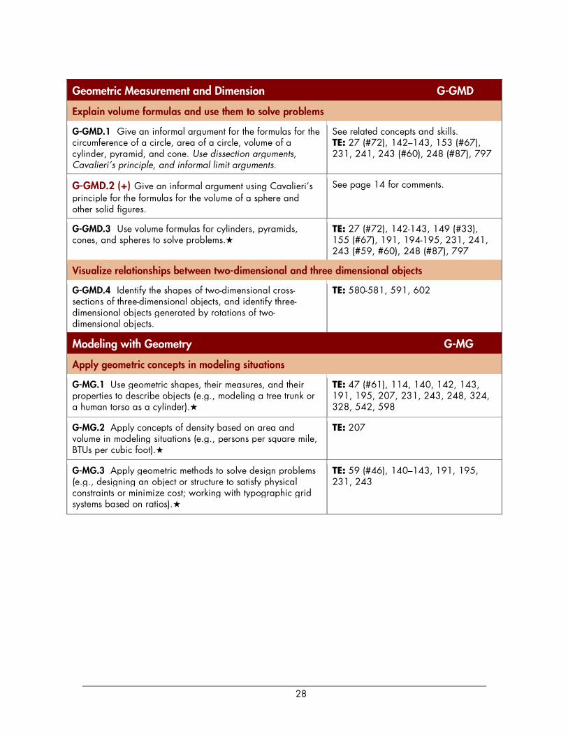
Geometric Measurement and Dimension G-GMD

Explain volume formulas and use them to solve problems

G-GMD.1 Give an informal argument for the formulas for the circumference of a circle, area of a circle, volume of a cylinder, pyramid, and cone. Use dissection arguments, Cavalieri’s principle, and informal limit arguments.

See related concepts and skills. TE: 27 (#72), 142–143, 153 (#67), 231, 241, 243 (#60), 248 (#87), 797

G-GMD.2 (+) Give an informal argument using Cavalieri’s principle for the formulas for the volume of a sphere and other solid figures.

See page 14 for comments.

G-GMD.3 Use volume formulas for cylinders, pyramids, cones, and spheres to solve problems.★

TE: 27 (#72), 142-143, 149 (#33), 155 (#67), 191, 194-195, 231, 241, 243 (#59, #60), 248 (#87), 797

Visualize relationships between two-dimensional and three dimensional objects

G-GMD.4 Identify the shapes of two-dimensional cross-sections of three-dimensional objects, and identify three-dimensional objects generated by rotations of two-dimensional objects.

TE: 580-581, 591, 602

Modeling with Geometry G-MG

Apply geometric concepts in modeling situations

G-MG.1 Use geometric shapes, their measures, and their properties to describe objects (e.g., modeling a tree trunk or a human torso as a cylinder).★

TE: 47 (#61), 114, 140, 142, 143, 191, 195, 207, 231, 243, 248, 324, 328, 542, 598

G-MG.2 Apply concepts of density based on area and volume in modeling situations (e.g., persons per square mile, BTUs per cubic foot).★

TE: 207

G-MG.3 Apply geometric methods to solve design problems (e.g., designing an object or structure to satisfy physical constraints or minimize cost; working with typographic grid systems based on ratios).★

TE: 59 (#46), 140–143, 191, 195, 231, 243

29

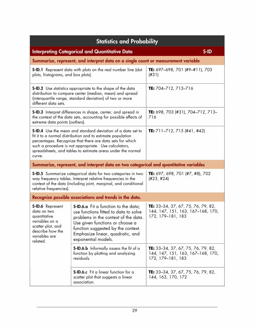
Statistics and Probability

Interpreting Categorical and Quantitative Data S-ID

Summarize, represent, and interpret data on a single count or measurement variable

S-ID.1 Represent data with plots on the real number line (dot plots, histograms, and box plots).

TE: 697–698, 701 (#9–#11), 703 (#31)

S-ID.2 Use statistics appropriate to the shape of the data distribution to compare center (median, mean) and spread (interquartile range, standard deviation) of two or more different data sets.

TE: 704–712, 713–716

S-ID.3 Interpret differences in shape, center, and spread in the context of the data sets, accounting for possible effects of extreme data points (outliers).

TE: 698, 703 (#31), 704–712, 713–716

S-ID.4 Use the mean and standard deviation of a data set to fit it to a normal distribution and to estimate population percentages. Recognize that there are data sets for which such a procedure is not appropriate. Use calculators, spreadsheets, and tables to estimate areas under the normal curve.

TE: 711–712, 715 (#41, #42)

Summarize, represent, and interpret data on two categorical and quantitative variables

S-ID.5 Summarize categorical data for two categories in two-way frequency tables. Interpret relative frequencies in the context of the data (including joint, marginal, and conditional relative frequencies).

TE: 697, 698, 701 (#7, #8), 702 (#23, #24)

Recognize possible associations and trends in the data.

S-ID.6.a Fit a function to the data; use functions fitted to data to solve problems in the context of the data. Use given functions or choose a function suggested by the context. Emphasize linear, quadratic, and exponential models.

TE: 33–34, 37, 67, 75, 76, 79, 82, 144, 147, 151, 163, 167–168, 170, 172, 179–181, 183

S-ID.6.b Informally assess the fit of a function by plotting and analyzing residuals.

TE: 33–34, 37, 67, 75, 76, 79, 82, 144, 147, 151, 163, 167–168, 170, 172, 179–181, 183

S-ID.6 Represent data on two quantitative variables on a scatter plot, and describe how the variables are related.

S-ID.6.c Fit a linear function for a scatter plot that suggests a linear association.

TE: 33–34, 37, 67, 75, 76, 79, 82, 144, 163, 170, 172

30

Interpret linear models

S-ID.7 Interpret the slope (rate of change) and the intercept (constant term) of a linear model in the context of the data.

TE: 29–30, 33, 34, 37, 38, 67, 75, 79, 163, 170, 172 (#67)

S-ID.8 Compute (using technology) and interpret the correlation coefficient of a linear fit.

TE: 146, 162, 163, 167, 179, 717–719, 725

S-ID.9 Distinguish between correlation and causation. TE: 162, 728 (#53)

Making Inferences and Justifying Conclusions S-IC

Understand and evaluate random processes underlying statistical experiments

S-IC.1 Understand statistics as a process for making inferences about population parameters based on a random sample from that population.

TE: 704, 719–720, 723–724, 726, 727, 728, 732

S-IC.2 Decide if a specified model is consistent with results from a given data-generating process, e.g., using simulation

TE: 719–728, 730, 731, 732

Make inferences and justify conclusions from sample surveys, experiments, and observational studies

S-IC.3 Recognize the purposes of and differences among sample surveys, experiments, and observational studies; explain how randomization relates to each.

TE: 719–728, 730, 731, 732

S-IC.4 Use data from a sample survey to estimate a population mean or proportion; develop a margin of error through the use of simulation models for random sampling.

TE: 720–721, 726 (#7–#12), 727 (#33, #34), 732 (#113, #114)

S-IC.5 Use data from a randomized experiment to compare two treatments; use simulations to decide if differences between parameters are significant.

TE: 721–723, 724–725, 726, 727, 728

S-IC.6 Evaluate reports based on data. TE: 695, 696, 697, 699–700, 701, 702, 703, 707, 708, 709, 710, 712, 733

31

Conditional Probability and the Rules of Probability S-CP

Understand independence and conditional probability and use them to interpret data

S-CP.1 Describe events as subsets of a sample space (the set of outcomes) using characteristics (or categories) of the outcomes, or as unions, intersections, or complements of other events (“or,” “and,” “not”).

TE: 661–662, 667 (#27, #28)

S-CP.2 Understand that two events A and B are independent if the probability of A and B occurring together is the product of their probabilities, and use this characterization to determine if they are independent.

TE: 661, 667 (#33, #34)

S-CP.3 Understand the conditional probability of A given B as P(A and B)/P(B), and interpret independence of A and B as saying that the conditional probability of A given B is the same as the probability of A, and the conditional probability of B given A is the same as the probability of B.

TE: 663–664, 667 (#31, #32)

S-CP.4 Construct and interpret two-way frequency tables of data when two categories are associated with each object being classified. Use the two-way table as a sample space to decide if events are independent and to approximate conditional probabilities.

Probability concepts are taught in Section 9.3. TE: 658–669

S-CP.5 Recognize and explain the concepts of conditional probability and independence in everyday language and everyday situations.

TE: 661–663, 666, 667

Use the rules of probability to compute probabilities of compound events in a uniform probability model

S-CP.6 Find the conditional probability of A given B as the fraction of B’s outcomes that also belong to A, and interpret the answer in terms of the model.

Conditional probability is introduced in Section 9.3. TE: 663

S-CP.7 Apply the Addition Rule, P(A or B) = P(A) + P(B) – P(A and B), and interpret the answer in terms of the model.

TE: 662

S-CP.8 (+) Apply the general Multiplication Rule in a uniform probability model, P(A and B) = P(A)P(B|A) = P(B)P(A|B), and interpret the answer in terms of the model.

TE: 663, 667 (#31, #32)

S-CP.9 (+) Use permutations and combinations to compute probabilities of compound events and solve problems.

TE: 658, 661, 666 (#5, #6), 667 (#33, #34)

32

Using Probability to Make Decisions S-MD

Calculate expected values and use them to solve problems

S-MD.1 (+) Define a random variable for a quantity of interest by assigning a numerical value to each event in a sample space; graph the corresponding probability distribution using the same graphical displays as for data distributions.

TE: 723–724, 727 (#33–#36) TK: 9.3.1, 9.3.2, 9.3.3, 9.3.7, 9.3.8

S-MD.2 (+) Calculate the expected value of a random variable; interpret it as the mean of the probability distribution.

TE: 668–669 (#61, #62) TK: 9.3.3, 9.3.4, 9.3.5, 9.3.6, 9.3.7, 9.3.8

S-MD.3 (+) Develop a probability distribution for a random variable defined for a sample space in which theoretical probabilities can be calculated; find the expected value.

TE: 659–660, 668 (#57, #61), 669 (#62) TK: 9.3.2, 9.3.3

S-MD.4 (+) Develop a probability distribution for a random variable defined for a sample space in which probabilities are assigned empirically; find the expected value.

TE: 659–660, 668 (#57, #61), 669 (#62) TK: 9.3.6, 9.3.7, 9.3.8

Use probability to evaluate outcomes of decisions

S-MD.5.a Find the expected payoff for a game of chance.

TE: 668–669 (#61, #62) TK: 9.3.3, 9.3.4, 9.3.5

S-MD.5 (+) Weigh the possible outcomes of a decision by assigning probabilities to payoff values and finding expected values.

S-MD.5.b. Evaluate and compare strategies on the basis of expected values.

TE: 668–669 (#61, #62) TK: 9.3.6, 9.3.7

S-MD.6 (+) Use probabilities to make fair decisions (e.g., drawing by lots, using a random number generator).

TE: 723–724, 727 (#33, #34)

S-MD.7 (+) Analyze decisions and strategies using probability concepts (e.g., product testing, medical testing, pulling a hockey goalie at the end of a game).

TE: 664, 667 (#34, #35, #38), 727–725, 732 (#113, #114) TK: 9.3.3, 9.3.4, 9.3.5, 9.3.6, 9.3.7

33

Closeness and Betweenness in a Complex World

An extension of Section 6.6

The real number line makes it easy to visualize closeness and betweenness in the world of real numbers, partly because the line represents an ordering of the real numbers, increasing from left to right along the line. The complex number system has some algebraic advantages (for example, we can factor any quadratic polynomial), but it has the disadvantage of not being orderable along a "complex number line." EXAMPLE 1 Proving that a Complex Number Line is Impossible Show that all three of these inequalities lead to contradictions according to the algebraic properties of order: i = 0, i > 0, i < 0. SOLUTION Suppose i = 0. Multiply both sides by i to get –1 = 0, a contradiction. Suppose i > 0. Multiply both sides by i to get –1 > 0, a contradiction. Suppose i < 0. Multiply both sides by i (remembering to switch the inequality because this time we are multiplying by a negative number) to get –1 > 0, a contradiction! This shows that you can't even put i on the same line with the real numbers and preserve the algebraic properties of order, so there can be no complex number line. Fortunately, we can still use the complex plane to understand closeness, as we hope you will discover in the following exploration.

We hope you concluded in the exploration above that the distance between two complex numbers x and y in the complex plane is, conveniently, x y! , just as it is for distance between two real numbers on the real line. In fact, we can make this a definition.

EXPLORATION 1 Measuring Closeness in the Complex Plane Which number is closer to 3 + 2i : 2 + 3i or 3 + 4i ? 1. Graph the three numbers in the complex plane and answer the question

graphically.

2. For real numbers, we measure the distance from x to y by x y! . Does this appear to work for complex numbers? (Be sure to use the definition of absolute value in Section 6.6.)

DEFINITION Distance Between Two Complex Numbers The distance between the complex numbers x and y is x y! . That is, if x a bi= + and y c di= + , then the distance between them is

2 2( ) ( ) ( ) ( )a c b d i a c b d! + ! = ! + ! .

34

The fact that the concept of "closeness" can be extended to the (unordered) complex numbers is more important than it might seem to you now. Calculus is explained by limits, and limits are explained by closeness. The main intent of a course called "precalculus" is to prepare you to study the calculus of real-valued functions, but if you go on to study the calculus of complex-valued functions you will revisit the connections you have made here. The concept of "betweenness" does not extend as nicely, because the very notion of betweenness should imply that the numbers are, in fact, lined up. One related concept that does extend naturally, however, is that of the mean of two numbers. Notice that the mean of two real numbers is represented on the real line by the midpoint of the segment between them:

Conveniently, the mean of two complex numbers is also represented in the complex plane by the midpoint of the segment between them:

x

y

x + y

2

This follows from the midpoint formula for two points in the plane. That is, if x a bi= + and

y c di= + , then ( ) ( )

2 2 2 2

x y a c b d i a c b di

+ + + + + +! " ! "= = +# $ # $

% & % &.

Although the picture is now two-dimensional, we would still say that the points on the segment connecting x and y "lie between" x and y. We can also extend this idea to other points in the complex plane, as the following example will show.

x y x + y 2

35

EXAMPLE 2 Extending the Concept of Betweenness a. Use an absolute value inequality to describe the set of real numbers that lie between

3 and 15. b. If the same absolute value inequality were to be used in the complex plane, what

numbers would lie between 3+ 2i and 9 + 10i ? SOLUTION a. The mean of 3 and 15 is 9, which is 6 units away from each number. The set of

numbers between 3 and 15 is described by 9 6x! < .

b. The mean of 3 + 2i and 9 + 10i is 6 + 6i, which is 2 2(6 3) (6 2) 5! + ! = units away

from each number. The inequality (6 6) 5z i! + < describes the interior of a circle of radius 5 in the complex plane around the point 6 + 6i.

This extends the algebraic and geometric concepts of betweenness in a natural way, but how should we describe it? It would be misleading to say that every point in the circle "lies between" 3 + 2i and 9 + 10i, as that should really describe the points on the connecting segment, even in higher dimensions. A more appropriate connection can be made using the concept of distance. The inequality in (a) describes the set of numbers on the real line whose distance is less than 6 units from the mean. Geometrically, their graph is an open line segment centered at the mean. The inequality in (b) describes the set of numbers in the complex plane whose distance is less than 6 units from the mean. Geometrically, their graph is the interior of a circle centered at the mean. We say that the points inside the circle form a "neighborhood" around the complex number 6 + 6i, just as the points in the open segment form a "neighborhood" around the real number 9. Neighborhoods will play an important role when you encounter limits of complex functions and limits of functions of several variables in future mathematics courses.

36

Exercises for “Closeness and Betweenness in a Complex World,” an extension of Section 6.6

1. Find the distance between 4 3i+ and 1 5i+ .

2. Which is closer to 8 3i+ , 2 i+ or 12 2i! ?

3. a. Accurately plot the complex numbers 2 4A i= ! ! , 1 1B i= + and 3 4C i= + .

b. Does B appear to lie on the line segment connecting A and C?

c. Find the distance between each pair of complex numbers in part (a).

d. What has to be true about the distances to ensure that B lies on the line segment between A and C?

4. Find a such that the distance between 7P a i= ! and 4 9Q i= ! ! is 6 units.

5. Find the midpoint between 8 10i! + and 4 3i+ .

6. a. Write an absolute value inequality to express the neighborhood of all complex numbers z that are closer to 6 i! than is the number 2 14i! + .

b. Write a brief geometric description of the neighbor expressed in 6a.

37

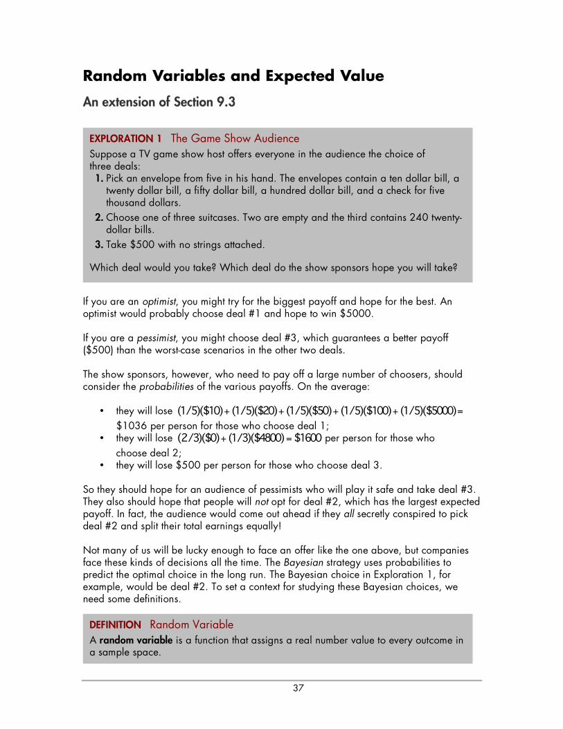
Random Variables and Expected Value

An extension of Section 9.3

If you are an optimist, you might try for the biggest payoff and hope for the best. An optimist would probably choose deal #1 and hope to win $5000. If you are a pessimist, you might choose deal #3, which guarantees a better payoff ($500) than the worst-case scenarios in the other two deals. The show sponsors, however, who need to pay off a large number of choosers, should consider the probabilities of the various payoffs. On the average:

• they will lose (1/5)($10) (1/5)($20) (1/5)($50) (1/5)($100) (1/5)($5000)+ + + + = $1036 per person for those who choose deal 1;

• they will lose (2/3)($0) (1/3)($4800) $1600+ = per person for those who choose deal 2;

• they will lose $500 per person for those who choose deal 3. So they should hope for an audience of pessimists who will play it safe and take deal #3. They also should hope that people will not opt for deal #2, which has the largest expected payoff. In fact, the audience would come out ahead if they all secretly conspired to pick deal #2 and split their total earnings equally! Not many of us will be lucky enough to face an offer like the one above, but companies face these kinds of decisions all the time. The Bayesian strategy uses probabilities to predict the optimal choice in the long run. The Bayesian choice in Exploration 1, for example, would be deal #2. To set a context for studying these Bayesian choices, we need some definitions.

EXPLORATION 1 The Game Show Audience Suppose a TV game show host offers everyone in the audience the choice of three deals: 1. Pick an envelope from five in his hand. The envelopes contain a ten dollar bill, a

twenty dollar bill, a fifty dollar bill, a hundred dollar bill, and a check for five thousand dollars.

2. Choose one of three suitcases. Two are empty and the third contains 240 twenty-dollar bills.

3. Take $500 with no strings attached.

Which deal would you take? Which deal do the show sponsors hope you will take?

DEFINITION Random Variable A random variable is a function that assigns a real number value to every outcome in a sample space.

38

It is convenient to denote random variables with capital letters and the individual values assumed by a random variable with subscripted lower-case letters. Thus X might be a random variable that takes on values { }1 2, , , nx x xK and Y might be a random variable

that takes on values { }1 2, , , ny y yK . We can then use the notation ( )P X to denote a probability function (Section 8.3) that assigns probabilities to the values of a random variable. We can describe the probability distribution with a table, as in Section 8.3. EXAMPLE 1 Probability Distribution of a Random Variable Let X be the random variable that gives the sum of the numbers on the top faces when two fair, 6-sided dice are rolled. Make a table showing the probability distribution for X. SOLUTION The values of X come from the sample space of all possible sums: {2, 3, 4, 5, 6, 7, 8, 9, 10, 11, 12}. The probability distribution is shown in Table 1.

X 2 3 4 5 6 7 8 9 10 11 12

P(X) 1/36 2/36 3/36 4/36 5/36 6/36 5/36 4/36 3/36 2/36 1/36 Table 1: Probability distribution for the total on two fair dice. Since probability functions of random variables are real-valued functions of real numbers, we can graph them in the coordinate plane. The most useful visualization is given by a histogram (Section 9.7) in which the heights of the rectangles are probabilities rather than frequencies. A histogram for the probability function in Example 1 is shown below. Note that we put the values of X in list

1L and the corresponding probabilities in list

2L .

MARGIN NOTE Seeing the Mean If you look at the histogram of the probability distribution, you should be able to see why the mean would be 7. You can estimate the mean of any probability distribution by visualizing the balancing point of its histogram along the horizontal axis, and that is easy to do with a symmetric distribution like this.

39

Like frequency distributions, probability functions have means and standard deviations. We can find them on a calculator as shown below:

In the case of a probability distribution, we give the mean a special name to suggest its significance in probability modeling.

EXAMPLE 2 Finding Expected Value For $5, a carnival huckster will let you draw a card at random from a fair deck of 52. He will pay you a dollar times the value of your card (ace = 1), but zero for a face card. What is the expected value of the payoff? Would you pay $5 to play this game? SOLUTION

1 1 1 1 1 1 1 1 1 1 3( ) 1 2 3 4 5 6 7 8 9 10 0

13 13 13 13 13 13 13 13 13 13 13

554.23

13

E X = ! + ! + ! + ! + ! + ! + ! + ! + ! + ! + !

= "

The expected value might not influence your decision to play or not play, but it is very important to the huckster, who can expect to make an average of 77 cents per game in the long run by charging $5 to play it You might get lucky playing once or twice, but the expected value shows that if you play this game for a long time at $5 per play, you can expect to lose an average of 77 cents per game. An important random variable in mathematical modeling is the random variable that counts the number of successes in n independent trials of an experiment with two possible outcomes. This random variable has a binomial probability distribution (as discussed in Section 9.3).

DEFINITION Expected Value of a Random Variable If X is a random variable with probability function P(X), the mean of the probability distribution is also called the mean of X (denoted

Xµ ) or the expected value of X

(denoted E(X)). Computationally, the expected value is the sum of the values of X

times their respective probabilities: 1

( ) ( )X k k

n

k

E X x P xµ=

= =! .

40

EXAMPLE 3 Expected Value and Binomial Distributions A fair coin is flipped five times. What is the expected number of heads? Interpret the expected value in the context of this example. SOLUTION If X is the random variable that counts the number of heads on five tosses, then X takes on the values {0,1, 2, 3, 4, 5} . Recall that the probabilities can be found by expanding the polynomial 5( )p q+ , where p is the probability of heads and q is the probability of tails (in this case, 1/2p q= = ).

5 5 4 3 2 2 3 4 5( ) 1 5 10 10 5 1

1 5 10 10 5 1

32 32 32 32 32 32

p q p p q p q p q pq q+ = + + + + +

= + + + + +

The expected value is 1 5 10 10 5 1( ) 0 1 2 3 4 5 2.5

32 32 32 32 32 32E X = ! + ! + ! + ! + ! + ! = .

This does not mean that we "expect" 2.5 heads when we toss the coin 5 times, as that is impossible. It does mean that if we perform the 5-toss experiment many times, the mean (or average) number of heads will be around 2.5. It is no coincidence that the expected value turned out to be half the number of tosses; in fact, that is the value you probably expected (pun unavoidable)! What number of heads would you expect on five tosses if the coin were weighted with the probability of heads equal to 3/5? If you would expect three, you would be right. We can state the general case as a theorem. EXAMPLE 4 A Chimpanzee Takes Organic Chemistry A chimpanzee is shown 100 questions from a multiple-choice test in Organic Chemistry. As each question appears on a screen, the chimpanzee presses one of four buttons to indicate the selected answer (A, B, C, or D). What is the chimpanzee's expected score? SOLUTION If we assume that the chimpanzee is unfamiliar with the material, the test amounts to 100 independent trials of a binomial experiment with probability ¼ of success. The expected number of correct answers is 100(1/4) = 25. Remember also that the expected value is really a mean, so a large class of chimpanzees would probably produce some scores higher than 25 (and, of course, some lower). An actual student taking this test should not conclude from a score of 25 that "Well, at least I showed that I knew 25% of the test." (See margin note.)

THEOREM Expected Value for a Binomial Distribution If X counts the number of successes on n independent trials of a binomial experiment with probability p of success, then ( )E X np= .

41

EXAMPLE 5 Playing the Lottery The payoff in your state lottery is up to 20 million dollars. To win, you must choose six numbers between 01 and 46 correctly. Optimistically, you purchase ten different lottery tickets at $2 each. What is the expected value of the game for you? SOLUTION The game rules will probably inform you that there are 9,366,819 possible lottery tickets of this type. You have ten of them, so your expected payoff in dollars is:

9366809 100 20,000,000 21.35

9366819 9366819! + ! " .

Unfortunately, you paid $20 for the tickets, bringing your expected profit down to $1.35. Probabilities in real life are often estimated rather than computed, but expected values can still guide Bayesian decision-making. EXAMPLE 6 The Warranty Extension For an extra $49 you can buy extended warranty protection on your new HDTV for three years. If the set requires maintenance during that time, it will be free. You estimate that there is a 5% chance that you might need a $300 repair within three years and a 1% chance that you will need a $500 repair, but the chances are 94% that you will need no repair at all. Based on expected values, should you purchase the extended coverage? SOLUTION If you DO purchase the coverage, your expected value (in dollars) is 49 0(0.94) 0(0.05) 0(0.01) 49! + + + = ! .

If you DO NOT purchase the coverage, your expected value (in dollars) is 0 0(0.94) ( 300)(0.05) ( 500)(0.01) 20+ + ! + ! = ! . The Bayesian strategy would be to decline the extended warranty and hope for the best. (The optimist would agree, while the pessimist would buy the coverage and avoid the possibility of those potential big losses.)

MARGIN NOTE The Guessing Penalty You may know that some standardized multiple-choice tests are scored with a "guessing penalty" that would bring the average chimpanzee's score down to zero. For a test with four options, as in Example 4, the formula would be 1

3R W! for R

right answers and W wrong answers. The chimp with the expected score of 25 would get an adjusted score of 1

325 (75) 0! = . Note that, under this grading system, a student who gets 25 right and leaves the other 75 blank would get an adjusted score of 25 and could justifiably claim to have known 25% of the test.

42

In most statistical applications, the probabilities used for real-world random variables are empirical probabilities (inferred from data) rather than theoretical probabilities (determined by the laws of probability). Expected values are determined using the same formula in either case and can be equally useful in decision-making. Looking at Example 6 from the other direction, the company offering the extended warranty must estimate those repair probabilities as accurately as they can so that they will know what to charge for the protection. They can track the repair bills incurred by a large number of customers and use a frequency table to compute the probabilities empirically, as in Example 7. EXAMPLE 7 A sample of 500 customers nationwide shows that they incurred repair bills in the first three years as recorded in Table 2:

Repair Bill Frequency 0 460

50 20 100 8 200 5 300 5 500 2

Table 2: A frequency table of 500 repair bills. If they charge each customer $29 for the extended warranty, what is their expected profit? SOLUTION We first approximate the probability distribution for the repair bills by dividing the frequencies by the sample size (500). The relative frequency table is shown in Table 3:

Repair Bill Probability 0 0.92

50 0.04 100 0.016 200 0.01 300 0.01 500 0.004

Table 3: A relative frequency table of 500 repair bills. The expected value in dollars is: 0(0.92) 50(0.04) 100(0.016) 200(0.01) 300(0.01) 500(0.004)+ + + + + = 10.60 If they charge $29 for the coverage, the expected profit per customer opting for the coverage is $29 – $10.60 = $18.40.

43

EXAMPLE 8 The Barber's Chair Bill the barber keeps a careful record of how long it takes him to cut the hair of 100 random customers during a typical week. The frequencies are recorded in Table 4:

Minutes in Chair Number of Customers 8 32 9 25

10 22 11 15 12 6

Table 4: Frequency table for the barber. What is the mean number of minutes a customer spends in Bill's chair? If there are four people waiting when he opens his shop, what is the expected time it will take for Bill to give all four of them haircuts? SOLUTION We begin by dividing the frequencies by the total number of customers, thus creating the empirical probability distribution shown in Table 5:

Minutes in Chair Probability 8 0.32 9 0.25

10 0.22 11 0.15 12 0.06

Table 5: Empirical probability table for the barber. Then ( ) 0.32(8) 0.25(9) 0.22(10) 0.15(11) 0.06(12)

9.38 minutes

E X = + + + +

=

Since it takes (on average) 9.38 minutes per customer, the expected length of time for Bill to cut the hair of four customers is 4(9.38) 37.52= minutes.

44

Exercises for “Random Variables and Expected Value,” an extension of Section 9.3

From the reading: 1. Make up an example of a random variable and specifically identify how it assigns

numbers to outcomes in the sample space.

2. What is a probability distribution?

3. Describe two ways to display a probability distribution.

4. What is another name for the mean of a probability distribution?

5. What is a simple way to calculate the mean of a binomial probability distribution?

6. Describe the difference between empirical probabilities and theoretical probabilities.

Applying the concepts: 7. A bag contains twenty numbered balls. Five of the balls have the number 1 on them.

Three balls have the number 2 on them. Seven balls have the number 3 on them. Four balls are marked with a 4. One ball has a 5 on it. Let Y be the random variable that gives the number on a ball chosen at random from the bag.

a. Show the probability distribution for Y in a table.

b. Calculate the expected value for Y.

8. One hundred people were asked how many televisions are in their home. The histogram below shows the empirical probability distribution of the results of the survey. The top of each bar corresponds to an integer multiple of 0.05. Calculate the expected value.

9. Not all dice are six-sided. If two ten-sided dice with faces numbered one through ten are rolled, what is the expected value for the sum of the dice?

0.05

0.15

1

0.25

2 3 4 5 7 6

45

10. At a carnival, people pay The Great Flubini $2 each to try to guess their weight within five pounds. If he guesses successfully, no prize is given. If he is off from five to ten pounds, participants get a prize worth $5. If he is off by more than ten pounds, participants get a $10 prize. The Great Fubini is correct 72% of the time, off from five to ten pounds 21% of the time and off by more than ten pounds 7% of the time. If The Great Fubini guesses the weights of 300 people per day, on average, is the carnival making money or losing money? How much per day?

11. A circular spinner consists of eight identical sectors. The spinner is equally likely to land in any of the eight sectors. Four of the eight yield no payout at all if the spinner lands there. Three of the eight pay $6 if the spinner lands there. One sector pays $10. It costs $5 to spin the spinner once. Use expected value to determine if it is a wise idea to play this game.

12. A game of chance consists of paying $4 to randomly draw a card from a deck of 50. The table below shows your chances of each net outcome. For example, 40% of the cards say, “You lose.” and so your net result is losing the $4 you paid to play. Complete the table below so that the game is a fair game. This means the expected value is 0.

X –4 –3 ? 2 4

P(X) 0.4 0.1 0.2 0.1 0.2

13. An unfair coin is one that is weighted so that the probability of getting heads does not equal the probability of getting tails. Suppose you have a coin weighted so it is likely to land on tails 60% of the time. Let X be the random variable that counts the number of tails obtained on four tosses.

a. Expand 4( )t h+ .

b. If t is the probability of tails and h is the probability of heads calculate the value of the term 3

4t h . What does the value represent?

c. Find the expected number of tails, E(X), using the polynomial.

d. Calculate the expected value using ( )E X np= .

14. Most people have dreamed of showing up to a final exam for a class they never attended. Marcel actually did this for his Mandarin language final exam, so he had to randomly guess on the 80-question multiple choice exam. Each question had 5 choices, A, B, C, D, or E, with only one answer being correct. Each question was worth one point.

a. What was the expected score for Marcel?

b. Explain why his actual score may have differed from his expected score.

46

15. From problem 14, suppose Marcel’s professor had imposed a “guessing penalty”

of 14

point off the final score for each incorrect answer. Would the adjusted score

have been a more accurate representation of his lack of Mandarin knowledge? Explain.

16. A multiple choice test consists of 150 questions each with n choices, where n is an integer greater than or equal to two. Each correct answer earns one point. Find the appropriate “guessing penalty” in terms of n so that the expected score for randomly guessing on all questions is zero.

17. A three year extended warranty on a laptop computer is offered for $79. Consumer reports show that typically, 4% of owners incur a $200 repair in that time and 1% of owners incur a $300 repair in that time. Does the extended warranty have a positive expected value for the consumer who purchases it? Show the work that leads to your conclusion.

18. The records of 1000 randomly selected customers of the XTREM car insurance company showed the following repair payouts by the company in the last fiscal year. What was the expected value of a payout?

Repair Payout (Dollars) Number

0 726

1000 83

2000 46

3000 52

4000 63

5000 17

6000 13

19. From problem 18, if the average annual premium payment collected from a customer was $1600, what was the company’s expected income per customer for extended warranties that year?

20. Make up a game of chance involving payment to play and payouts, and compute the expected value of the game for the player.

47

ANSWER SETS Answers to the exercises for “Closeness and Betweenness in a Complex World”

1. 13

2. 2 i+ is closer because 40 41< .

3. a.

b. Yes, B appears to lie on the line segment between A and C.

c. 34AB = , 13BC = , 89AC =

d. AB BC AC+ = (So B is not on the line segment between A and C.)

4. 4 4 2a = ! + or 4 4 2a = ! !

5. 132

2i! +

6. a. (6 ) 17z i! ! <

b. The neighborhood includes all points within a circle of radius 17 around the complex number 6 i! .

!6 !5 !4 !3 !2 !1 1 2 3 4 5 6

!4

!3

!2

!1

1

2

3

4

R

i

A

B

C

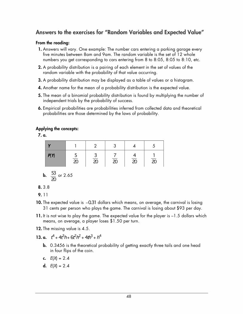
48

Answers to the exercises for “Random Variables and Expected Value”

From the reading: 1. Answers will vary. One example: The number cars entering a parking garage every

five minutes between 8am and 9am. The random variable is the set of 12 whole numbers you get corresponding to cars entering from 8 to 8:05, 8:05 to 8:10, etc.

2. A probability distribution is a pairing of each element in the set of values of the random variable with the probability of that value occurring.

3. A probability distribution may be displayed as a table of values or a histogram.

4. Another name for the mean of a probability distribution is the expected value.

5. The mean of a binomial probability distribution is found by multiplying the number of independent trials by the probability of success.

6. Empirical probabilities are probabilities inferred from collected data and theoretical probabilities are those determined by the laws of probability.

Applying the concepts: 7. a.

b. 53

20 or 2.65

8. 3.8

9. 11

10. The expected value is 0.31! dollars which means, on average, the carnival is losing 31 cents per person who plays the game. The carnival is losing about $93 per day.

11. It is not wise to play the game. The expected value for the player is –1.5 dollars which means, on average, a player loses $1.50 per turn.

12. The missing value is 4.5.

13. a. 4 3 2 2 3 44 6 4t t h t h th h+ + + +

b. 0.3456 is the theoretical probability of getting exactly three tails and one head in four flips of the coin.

c. E(X) = 2.4

d. E(X) = 2.4

Y 1 2 3 4 5

P(Y) 5

20

3

20

7

20

4

20

1

20

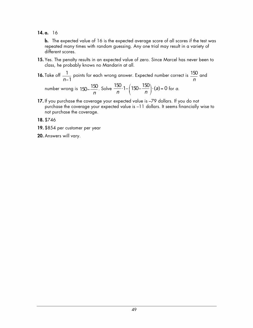
49

14. a. 16

b. The expected value of 16 is the expected average score of all scores if the test was repeated many times with random guessing. Any one trial may result in a variety of different scores.

15. Yes. The penalty results in an expected value of zero. Since Marcel has never been to class, he probably knows no Mandarin at all.

16. Take off 1

1n! points for each wrong answer. Expected number correct is 150

n and

number wrong is 150150

n! . Solve

150 1501 150 ( ) 0a

n n

! "# $ $ # =% &

' ( for a.

17. If you purchase the coverage your expected value is –79 dollars. If you do not purchase the coverage your expected value is –11 dollars. It seems financially wise to not purchase the coverage.

18. $746

19. $854 per customer per year

20. Answers will vary.