Delft University of TechnologyFaculty of Electrical Engineering, Mathematics and Computer Science

Delft Institute of Applied Mathematics

Implementation of the Deflated PreconditionedConjugate Gradient Method for Bubbly Flow on

the Graphical Processing Unit(GPU)

A thesis submitted to theDelft Institute of Applied Mathematicsin partial fulfillment of the requirements

for the degree

MASTER OF SCIENCEin

COMPUTER ENGINEERING

by

Rohit Gupta

Delft, the NetherlandsAugust 2010

Copyright c© 2010 by Rohit Gupta. All rights reserved.

MSc THESIS COMPUTER ENGINEERING

“Implementation of the Deflated Preconditioned Conjugate Gradient Methodfor Bubbly Flow on the

Graphical Processing Unit(GPU)”

ROHIT GUPTA

Delft University of Technology

Daily supervisors Responsible professor

Prof. dr. ir. C. Vuik Prof. dr. ir. H.J. SipsIr. C.W.J. Lemmens

Other thesis committee member(s)

Dr. ir. M.B. van Gijzen

August 2010 Delft, the Netherlands

Abstract

In this work we have implemented the Iterative Method of Conjugate Gradients with twolevels of Preconditioning to solve a System of Linear Equations on Graphical ProcessingUnit(GPU). This system represents the discretized Pressure equation resulting from the

Level Set Method Solution of the Incompressible Navier Stokes Equation used tocompute Bubbly Flows. We have tried to explore the problem space with different grid

sizes, number of preconditioning blocks and deflation vectors. The results show thatwhen the methods for preconditioning are chosen so that they can exhibit ample

parallelism we can achieve considerable performance up to 20 times better than the CPUversion. We show in our analysis that we are very close to maximum achievable speedup.We also report on the accuracy of our results and argue that GPUs can be beneficial in

solving such problems efficiently.

iii

Acknowledgments

I thank God :). I thank My Family for their blessings and I thank my supervisors forhelping me and trusting me to complete this work.

Contents

1 Introduction 1

2 Problem Definition 22.1 Formulating the Problem for Two-Phase Flow . . . . . . . . . . . . . . . . . 2

3 Iterative Methods for Linear Systems 53.1 Conjugate Gradient . . . . . . . . . . . . . . . . . . . . . . . . . . . . . . . 7

3.1.1 Arnoldi Orthogonalization . . . . . . . . . . . . . . . . . . . . . . . . 83.1.2 Lanczos Method . . . . . . . . . . . . . . . . . . . . . . . . . . . . . 83.1.3 Conjugate Gradient Algorithm . . . . . . . . . . . . . . . . . . . . . 9

3.2 Preconditioning . . . . . . . . . . . . . . . . . . . . . . . . . . . . . . . . . . 123.2.1 Incomplete Cholesky Preconditioning . . . . . . . . . . . . . . . . . . 133.2.2 Incomplete Poisson Preconditioning . . . . . . . . . . . . . . . . . . 13

3.3 Deflation . . . . . . . . . . . . . . . . . . . . . . . . . . . . . . . . . . . . . 163.3.1 Subdomain Deflation . . . . . . . . . . . . . . . . . . . . . . . . . . . 18

4 GPU for Scientific Computing 184.1 Device Architecture . . . . . . . . . . . . . . . . . . . . . . . . . . . . . . . 18

4.1.1 Execution Configuration . . . . . . . . . . . . . . . . . . . . . . . . . 194.1.2 Execution of Threads . . . . . . . . . . . . . . . . . . . . . . . . . . 204.1.3 Memory Model . . . . . . . . . . . . . . . . . . . . . . . . . . . . . . 21

4.2 Language Extensions . . . . . . . . . . . . . . . . . . . . . . . . . . . . . . . 214.3 Methods of reducing code execution times . . . . . . . . . . . . . . . . . . . 21

5 Previous Work 225.1 Solving Linear Systems on the GPU . . . . . . . . . . . . . . . . . . . . . . 23

5.1.1 Prefix Scan for calculating sum . . . . . . . . . . . . . . . . . . . . . 235.1.2 Sparse Matrix Vector Products- SpMVs . . . . . . . . . . . . . . . . 24

5.2 Conjugate Gradient . . . . . . . . . . . . . . . . . . . . . . . . . . . . . . . 255.3 Preconditioning . . . . . . . . . . . . . . . . . . . . . . . . . . . . . . . . . . 255.4 Precision Improvement . . . . . . . . . . . . . . . . . . . . . . . . . . . . . . 265.5 Other Important Approaches . . . . . . . . . . . . . . . . . . . . . . . . . . 27

6 Implementation 276.1 SpMV Kernel . . . . . . . . . . . . . . . . . . . . . . . . . . . . . . . . . . . 286.2 Preconditioning Kernel . . . . . . . . . . . . . . . . . . . . . . . . . . . . . . 286.3 Deflation Kernels . . . . . . . . . . . . . . . . . . . . . . . . . . . . . . . . . 29

7 Optimizations and Results 297.1 Conjugate Gradient - Vanilla Version . . . . . . . . . . . . . . . . . . . . . . 29

7.1.1 Code Commentary . . . . . . . . . . . . . . . . . . . . . . . . . . . . 297.1.2 Comparisons with GPU versions . . . . . . . . . . . . . . . . . . . . 317.1.3 Profiler Picture . . . . . . . . . . . . . . . . . . . . . . . . . . . . . . 32

7.2 Diagonal Preconditioning . . . . . . . . . . . . . . . . . . . . . . . . . . . . 337.3 Conjugate Gradient with Preconditioning . . . . . . . . . . . . . . . . . . . 33

7.3.1 Code Commentary . . . . . . . . . . . . . . . . . . . . . . . . . . . . 337.3.2 Comparisons with GPU versions . . . . . . . . . . . . . . . . . . . . 337.3.3 Profiler Picture . . . . . . . . . . . . . . . . . . . . . . . . . . . . . . 35

7.4 Conjugate Gradient with Deflation and Preconditioning-Block IC . . . . . . 367.4.1 Code Commentary . . . . . . . . . . . . . . . . . . . . . . . . . . . . 367.4.2 Comparisons with GPU versions . . . . . . . . . . . . . . . . . . . . 37

i

7.4.3 Profiler Picture . . . . . . . . . . . . . . . . . . . . . . . . . . . . . . 397.5 Conjugate Gradient with Deflation and Preconditioning - AZ storage opti-

mized . . . . . . . . . . . . . . . . . . . . . . . . . . . . . . . . . . . . . . . 397.5.1 Comparisons with GPU versions . . . . . . . . . . . . . . . . . . . . 437.5.2 Profiler Picture . . . . . . . . . . . . . . . . . . . . . . . . . . . . . . 43

7.6 Conjugate Gradient with Deflation and IP Preconditioning - AZ storageoptimized . . . . . . . . . . . . . . . . . . . . . . . . . . . . . . . . . . . . . 457.6.1 Comparisons with GPU versions . . . . . . . . . . . . . . . . . . . . 457.6.2 Profiler Picture . . . . . . . . . . . . . . . . . . . . . . . . . . . . . . 47

7.7 Conjugate Gradient with Deflation and IP Preconditioning - AZ storageoptimized and optimized Matrix Vector ( E−1b) Multiplication . . . . . . . 477.7.1 Comparisons with GPU versions . . . . . . . . . . . . . . . . . . . . 477.7.2 Profiler Picture . . . . . . . . . . . . . . . . . . . . . . . . . . . . . . 50

8 Experiments with Two Phase Flow Matrix 508.1 Conjugate Gradient -Vanilla Version and with Block- IC and Diagonal Pre-

conditioning . . . . . . . . . . . . . . . . . . . . . . . . . . . . . . . . . . . 508.1.1 Comparisons with GPU versions . . . . . . . . . . . . . . . . . . . . 54

8.2 Conjugate Gradient with Deflation and Block-IC Preconditioning . . . . . . 548.3 Conjugate Gradient with Deflation and IP Preconditioning . . . . . . . . . 59

9 Analysis 599.1 Static Analysis . . . . . . . . . . . . . . . . . . . . . . . . . . . . . . . . . . 599.2 Kernels- Performance . . . . . . . . . . . . . . . . . . . . . . . . . . . . . . . 649.3 Bandwidth Utilization . . . . . . . . . . . . . . . . . . . . . . . . . . . . . . 659.4 Discussion on Possible Speedup Limits . . . . . . . . . . . . . . . . . . . . . 67

9.4.1 Summary . . . . . . . . . . . . . . . . . . . . . . . . . . . . . . . . . 68

10 Future Work and Conclusions 68

A How the Appendix is organized 73

B Grid, Matrix, Blocks, Domains, Matrices 73B.1 The Grid . . . . . . . . . . . . . . . . . . . . . . . . . . . . . . . . . . . . . 73B.2 The Matrix . . . . . . . . . . . . . . . . . . . . . . . . . . . . . . . . . . . . 74B.3 Blocks for Incomplete Cholesky . . . . . . . . . . . . . . . . . . . . . . . . . 74B.4 Domains for Deflation . . . . . . . . . . . . . . . . . . . . . . . . . . . . . . 74B.5 Coefficients in different types of Matrices . . . . . . . . . . . . . . . . . . . 74

B.5.1 Poisson Type . . . . . . . . . . . . . . . . . . . . . . . . . . . . . . . 74B.5.2 Two-Phase Matrix . . . . . . . . . . . . . . . . . . . . . . . . . . . . 74

C Detailed Results 78C.1 Poisson Type . . . . . . . . . . . . . . . . . . . . . . . . . . . . . . . . . . . 78

C.1.1 Deflated CG-with Block Incomplete Cholesky Preconditioning . . . 78C.2 Two Phase . . . . . . . . . . . . . . . . . . . . . . . . . . . . . . . . . . . . 78

C.2.1 Deflated CG-with Block Incomplete Cholesky Preconditioning . . . 78

ii

1 Introduction

Computations of Bubbly flows is the main application for this implementation. Under-standing the dynamics and interaction of bubbles and droplets in a large variety of pro-cesses in nature, engineering, and industry are crucial for economically and ecologicallyoptimized design. Bubbly flow occur, for example, in chemical reactors, boiling, fuelinjectors, coating and volcanic eruptions.

Two phase flows are complicated to simulate, because the geometry of the problemtypically varies with time, and the fluids involved have very different material properties.Following from the previous work [Tang, 2008] we consider stationary and time-dependentbubbly flows, where the computational domain is always a unit square or unit cube filledwith a fluid to a certain height. The bubbles and droplets in the domain are always chosensuch that they are located in a structured way and have equal radius, at the starting time.

Mathematically bubbly flows are modeled using the Navier Stokes equations includingboundary and interface conditions, which can be approximated numerically using operatorsplitting techniques. In these schemes, equations for the velocity and pressure are solvedsequentially at each time step. In many popular operator-splitting methods, the pressurecorrection is formulated implicitly, requiring the solution of a linear system (3) at eachtime step. This system takes the form of a Poisson equation with discontinuous coefficients(also called the ’pressure(-correction) equation’) and Neumann boundary conditions, i.e.,

−5 .

(1

ρ(x)5 p(x)

)= f(x), x ∈ Ω, (1)

∂

∂np(x) = g(x), x ∈ ∂Ω, (2)

where Ω, p, ρ, x and n denote the computational domain, pressure, density, spatialcoordinates, and the unit normal vector to the boundary, ∂Ω, respectively. Right-handsides f and g follow explicitly from the operator-splitting method, where g is such thatmass is conserved, leading to a singular but compatible linear system (3).

In this work we look at the implementation of a numerical solution of a Linear PartialDifferential Equation (PDE), resulting from the mathematical modeling of bubbly flows.The PDEs have been discretized through the use of finite differences. A Linear Sytemarises from such a discretization. We are interested in systems of the form,

Ax = b, A ∈ Rn×n, n ∈ N (3)

where n is the number of degrees of freedom and is also called the dimension of A. AlsoA is symmetric positive definite(SPD), i.e.,

A = AT , yTAy > 0 ∀ y ∈ R y 6= 0. (4)

The linear system given by (3) is usually sparse and ill-conditioned. This means thatthere are few non-zero elements per row of A and also that the condition number κ(A)is usually large. Put in other words, the ratio of the largest eigenvalue to the smallest islarge and this leads to slow convergence of the Conjugate Gradient Method.

κ(A) : =λnλ1

(5)

where 0 < λ1 ≤ λ2 ≤ ... ≤ λn are eigenvalues of matrix A.Solving the system (3) by direct methods is also an option but it is usually not memory-

wise or computationally efficient. Though these methods are robust and generally appli-cable but they also tend to be prohibitively expensive. The sparsity of the matrix A

1

necessitates the use of efficient storage methods and computation with ’iterative meth-ods’. The term ’iterative method’ refers to a wide range of techniques that use iterates,or successive approximations to obtain more accurate solutions to a linear system at eachiteration step.

Krylov subspace methods, especially the Conjugate Gradient Method is the prominentchoice for solving such systems. However the convergence of this method depends heavilyon κ(A). In order to avoid more and more iterations, as κ(A) rises with increasing problemsizes, the matrix A is preconditioned to bring down the condition number form κ(A) to

κ(M−12 AM

12 ) which is equivalent to κ(M−1A). The coefficient matrix A is multiplied by

M−1, the preconditioner. The original system (3) then looks like,

M−1Ax = M−1b, (6)

where M is symmetric and positive definite just like A. M−1 is chosen in such a waythat the cost of the operation M−1y with a vector y is computationally cheap. However,sometimes preconditioning might also not be enough. In that case we use second level ofpreconditioning or Deflation in order to reduce κ(A). In this work some previous results[Tang, 2008] are used for implementation. The focus is to implement these methods onthe Graphical Processing Unit (GPU).

Recently Scientific Computing has largely benefited from the data parallel architectureof graphical processors. Many interesting problems which are computationally intensiveare ideally suited to the GPU, especially matrix calculations. It is only intuitive to usethem for solution of discretized partial equations. With the advent of the ComponentUnified Device Architecture (CUDA) paradigm of computing available on NVIDIA GPUdevices, it has become easier to write such applications. More time can be spent in explor-ing the ’What If?’ scenarios that are of scientific importance rather than understandingdevice specifics. We briefly define the problem of Bubbly flows followed by a backgroundon Iterative Methods. Subsequently we introduce the Parallelization of Iterative meth-ods. After introducing some of the Architectural details of the GPU and and a glimpseof the programming techniques we discuss the recent work that has been done on theGPU with respect to solving iteratively the linear systems emerging from discretization ofPDEs. Then we present an overview of the Implementation followed by the results fromthe Numerical Experiments. Further, we analyze our results and we end this report witha conclusion.

2 Problem Definition

Solving the linear system (3), that is a discretization of (1), within an operator splittingapproach is a bottleneck in the fluid-flow simulation, since it typically consumes the bulkof the computing time. In order to accelerate the calculation of the solution by the Precon-ditioned Conjugate Gradient Algorithm with deflation we propose to use the GPU. Thechallenge lies in optimizing the computation on the GPU in such a way so as to extractthe maximum computation throughput it can deliver. This requires exploring Algorith-mic enhancements and Architectural provisions to achieve the best possible performancespeedup.

2.1 Formulating the Problem for Two-Phase Flow

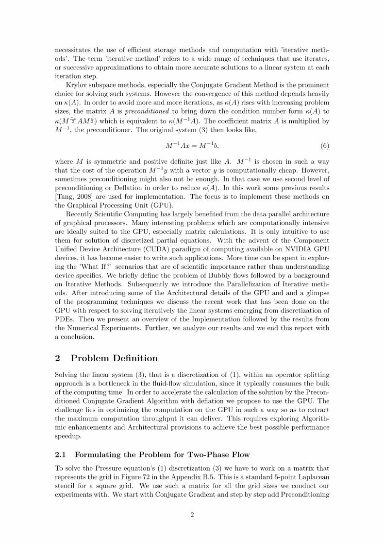
To solve the Pressure equation’s (1) discretization (3) we have to work on a matrix thatrepresents the grid in Figure 72 in the Appendix B.5. This is a standard 5-point Laplaceanstencil for a square grid. We use such a matrix for all the grid sizes we conduct ourexperiments with. We start with Conjugate Gradient and step by step add Preconditioning

2

ρ = 1000

ρ =1

Figure 1: Two phase Flow Computational Model

and Deflation to it. For the 5-point Laplacean matrix we do not see any change in diagonalpreconditioning since the coefficients are not having any discontinuities.

However when we consider the matrix for a two phase problem then instead of thesmooth coefficients on the diagonals we have big jumps or discontinuities in the matrix.Table B.5.2 in the Appendix B.5 lists a part of the Two Phase Matrix (Density Contrast1000 : 1). This is attributed to the large difference in the densities of the two fluids weare trying to model. Now we explain how we arrive on this kind of a matrix.

First let us take a look at the picture (Figure 1) of the problem in terms of an interfaceand two mediums with Neumann Boundary Conditions.

When we discretize the problem, a grid results which has coefficients placed on the 5diagonals with the jumps appearing at the interface region. We follow a mass conservingapproach (as shown in Figure 2) while calculating the coefficients on the interface.

There is some flux that enters horizontally and vertically and some of it leaves a cell.By taking the cell-centered approach (wherein the discretization point is at the center ofthe cell) and taking into account the contribution of all the flows through that point wearrive on a stencil.

The stencils for the cells which are not on the interfaces are straightforward to calculate.

3

Figure 2: Flux entering and leaving a discretized cell

4

Figure 3: 8× 8 grid with two mediums and an interface.

Below we briefly talk about the points on the interface and how we calculated their stencils.Consider the model grid of dimension 8 × 8 in which we have a point that lies on

the interface and also adjoining the boundary. The cell is highlighted with a thick blackborder in the Figure 3.

Refer to the Flux picture as shown in Figure 2. For example if we consider the left cellwith co-ordinates ((i − 1), j) to be on the boundary (the gray colored section in Figure1 ). Then there is no flux coming in from the horizontal direction however since the cell((i + 1), j) is inside (not adjoining the boundary) we have some flux going out. In thevertical direction we have flux coming in from the the point (i, (j − 1)) and flux going outfrom the cell (i, (j + 1)). Keeping these in mind and assuming that the density ratio ofthe rarer medium (orange) to the denser medium is ε. We can write for this point

1

h[−Pi,j−1 − εP(i, j + 1)− (

1

2+

1

2ε)Pi+1,j + (1

1

2+ 1

1

2ε)Pi,j ] (7)

where h is the dimension of a cell i.e. 1n for a n×n grid. Further we can get the stencil

[−1 0 (11

2+ 1

1

2ε) (−1

2− 1

2ε) −ε]. (8)

Deriving stencils in this way the complete matrix (as provided in Table B.5.2 in theAppendix B.5) for this 8× 8 grid can be worked out.

3 Iterative Methods for Linear Systems

There are a variety of methods to approximate a solution to the system

Ax = b (9)

where x is an unknown vector, b is a known vector, and A is a known matrix ofcoefficients. To begin we consider two basic methods.

These methods might take a large number of iterations to converge to a solution andmight not be useful as standalone solvers.

Jacobi Method

5

The Jacobi iteration is based on the idea of splitting up A into D, E and F.

A = D − E − F (10)

in which D is the diagonal of A, −E its strict lower part, and −F its strict upper part, Itis always assumed that the diagonal entries of A are all nonzero.

The Jacobi iteration determines the i−th component of the next approximation so asto annihilate the i−th component of the residual vector. In the following, ξi denotes thei−th component of the iterate xk and βi the i−th component of the right-hand side b.Thus, writing

(b−Axk+1)i = 0 (11)

in which (y)i represents the i−th component of the vector y, yields

aiiξ(k+1)i = −

n∑j=1,j 6=1

aijξ(k)j + βi, (12)

or

ξ(k+1)i =

1

aii

(βi −

n∑j=1j 6=1

aijξ(k)j

)i = 1, ..., n (13)

This is a component-wise form of the Jacobi iteration. All components of the nextiterate can be grouped into the vector xk+1. The above notation can be used to rewritethe Jacobi iteration (13) in vector form as

xk+1 = D−1(E + F )xk +D−1b (14)

Gauss-Seidel

The Gauss-Seidel iteration corrects the i−th component of the current approximate solu-tion, in the order i = 1, 2, ..., n , again to annihilate the i−th component of the residual.However, this time the approximate solution is updated immediately after the new com-

ponent is determined. The newly computed components ξ(k)i , i = 1, 2, ..., n can be changed

within a working vector which is redefined at each relaxation step. Thus, since the orderis i = 1, 2, ..., n, the result at the i−th step is

βi −i−1∑j=1

aijξ(k+1)j − aiiξ(k+1)

i −n∑

j=i+1

aijξ(k)j = 0, (15)

which leads to the iteration,

ξ(k+1)i =

1

aii

(−

i−1∑j=1

aijξ(k+1)j −

n∑j=i+1

aijξ(k)j + βi

), i = 1, ..., n (16)

the defining equation (15) can be written as

b+ Exk+1 −Dxk+1 + Fxk = 0, (17)

which leads immediately to the vector form of the Gauss-Seidel iteration

xk+1 = (D − E)−1Fxk + (D − E)−1b. (18)

6

Computing the new approximation in (14) requires multiplying by the inverse of thediagonal matrix D. In (18) a triangular system must be solved with D−E, the lower tri-angular part of A. Thus, the new approximation in a Gauss-Seidel step can be determinedeither by solving a triangular system with the matrix D − E or from the relation (15).

A backward Gauss-Seidel iteration can also be defined as

(D − F )xk+1 = Exk + b, (19)

which is equivalent to making the coordinate corrections in the order n, n − 1, ..., 1.A Symmetric Gauss-Seidel Iteration consists of a forward sweep followed by a backwardsweep. The Jacobi and the Gauss-Seidel iterations are both of the form

Mxk+1 = Nxk + b = (M −A)xk + b, (20)

in whichA = M −N (21)

is a splitting of A , with M = D for Jacobi, M = D−E for forward Gauss-Seidel,andM = D − F for backward Gauss-Seidel.

Writing in terms of the solution vector xk at the kth iteration we have the Jacobi andGauss-Seidel iterations look like the form

xk+1 = Gxk + f, (22)

in which

GJA(A) = I −D−1A (23)

GGS(A) = I − (D − E)−1A, (24)

for the Jacobi and Gauss-Seidel iterations, respectively.

3.1 Conjugate Gradient

The Conjugate Gradient method is an important method for solving sparse linear systems.It is based on the idea of using a projection method on Krylov Subspaces Km to find anapproximate solution xm to

Ax = b (25)

This is in turn done by imposing a Petrov Galerkin condition

b−Axm⊥Lm, (26)

where Lm is another subspace of dimension m. Here, x0 represents an arbitrary initialguess to the solution. The subspace Km is written as

Km(A, r0) = spanr0, Ar0, A2r0, ..., Am−1r0, (27)

where r0 = b−Ax0.When there is no ambiguity, Km(A, r0)will be denoted by Km. The different versions

of Krylov subspace methods arise from different choices of the subspace Lm and from theways in which the system is preconditioned.

Two broad choices for Lm give rise to the best known techniques. The first is simplyLm = Km and the minimum-residual variation Lm = AKm.

An important assumption, for The Conjugate Gradient Method, is that the coefficientmatrix A is Symmetric Positive Definite(SPD).

7

3.1.1 Arnoldi Orthogonalization

The Arnoldi method is an orthogonal projection method ontoKm for general non-Hermitianmatrices. The procedure was introduced in 1951 as a means of reducing a dense matrixinto Hessenberg form. Arnoldi presented his method in this manner but hinted that theeigenvalues of the Hessenberg matrix obtained from a number of steps smaller than n couldprovide accurate approximations to some eigenvalues of the original matrix. It was laterdiscovered that this strategy leads to an efficient technique for approximating eigenvaluesof large sparse matrices.

Algorithm 1 Arnoldi Orthogonalization

1: Choose a vector v1 of norm 12: for For j = 1, 2, ...m do3: Compute hij = (Avj , vi) for i = 1, 2, ..., j

4: Compute wj := Avj −∑j

i=1 hijvi5: hj+1,j = ‖wj‖26: if hj+1,j = 0 then7: Stop8: end if9: vj+1 = wj/hj+1,j

10: end for

At each step, the Algorithm 1 multiplies the previous Arnoldi vector vj by A andthen orthonormalizes the resulting vector wj against all previous vis by a standard Gram-Schmidt procedure. It stops if the vector wj vanishes.

3.1.2 Lanczos Method

The symmetric Lanczos algorithm can be viewed as a simplification of the Arnoldi methodfor the particular case when the matrix is symmetric. When A is symmetric, then the Hes-senberg matrix Hm becomes symmetric tridiagonal. This leads to a three-term recurrencein the Arnoldi process and short-term recurrences for solution algorithms such as FOMand GMRES. The standard notation used to describe the Lanczos algorithm is obtainedby setting

αj ≡ hij , βj ≡ hj−1,j , (28)

and if Tm denotes the resulting Hm matrix, it is of the form,

Tm =

α1 β2β2 α2 β3

· · ·βm−1 αm−1 βm

βm αm

. (29)

This leads to the Lanczos algorithm specified in Algorithm 2.It is rather surprising that the above simple algorithm guarantees, at least in exact

arithmetic, that the vectors vi, i = 1, 2, ..., are orthogonal. In reality, exact orthogonalityof these vectors is only observed at the beginning of the process. At some point the visstart losing their global orthogonality rapidly. The major practical differences with theArnoldi method are that the matrix Hm is tridiagonal and, more importantly, that onlythree vectors must be stored, unless some form of re-orthogonalization is employed.

8

Algorithm 2 Lanczos Algorithm

1: Choose an initial vector v1 of norm unity. Set β1 ≡ 0, v0 ≡ 02: for j = 1, 2, ...,m do3: wj := Avj − βjvj−14: αj := (wj , vj)5: wj := wj − αjvj6: βj+1 := ‖wj‖27: if βj+1 = 0 then8: Stop9: end if

10: vj+1 := wj/βj+1.11: end for

3.1.3 Conjugate Gradient Algorithm

The Conjugate Gradient method is a realization of an orthogonal projection techniqueonto the Krylov Subspace Km(A, r0) where, r0 is the initial residual.

First we derive the Arnoldi Method for the case when A is symmetric. Given an initialguess x0 to the linear system Ax = b and the Lanczos vectors vi, i = 1, ...,m togetherwith the tridiagonal matrix Tm, the approximate solution obtained from an orthogonalprojection method onto Km, is given by

xm = x0 + Vmym, ym = T−1m (βe1). (30)

We now have the Lanczos method for linear systems in Algorithm 3. We can write LU

Algorithm 3 Lanczos Method for Linear Systems

1: Compute r0 = b−Ax0, β : = ‖r0‖2, and v1 : = r0/β2: for j = 1, 1, ...,m do3: wj = Avj − βjvj−1( If j = 1 set β1v0 ≡ 0)4: αj = (wj , vj)5: wj := wj − αjvj6: βj+1 = ‖wj‖27: if βj+1 = 0 then8: set m : = j and go to 99: end if

10: vj+1 = wj/βj+1

11: end for12: Set Tm = tridiag (βi, αi, βi+1), and Vm = [v1, ..., vm].13: Compute ym = T−1m (βe1) and xm = x0 + Vmym

factorization of Tm as Tm = LmUm. The matrix Lm is unit lower bi-diagonal and Um isupper bi-diagonal. Thus, the factorization of Tm is of the form

Tm =

1λ2 1

λ3 1λ4 1

λ5 1

×η1 β2

η2 β3η3 β4

η4 β5η5

. (31)

The approximate solution is then given by,

xm = x0 + VmU−1m L−1m (βe1). (32)

9

Letting

Pm ≡ VmU−1m (33)

andzm = L−1m βe1, (34)

then,xm = x0 + Pmzm. (35)

Note that, pm, the last column of Pm, can be computed from the previous pi’s and vmby the simple update

pm = η−1[vm − βmpm−1]. (36)

Here βm is a scalar computed from the Lanczos Algorithm, while ηm results from the m-thGaussian Elimination step on the tridiagonal matrix, i.e.,

λm =βmηm−1

, (37)

ηm = αm − λmβm. (38)

Also from the structure of Lm we have

zm =

[zm−1ζm

], (39)

in which ζm = −λmζm−1. As a result, xm can be updated at each step as

xm = xm−1 + ζmpm (40)

where pm is defined above.This brings us to the direct version of Lanczos algorithm for linear systems.

Algorithm 4 D-Lanczos

1: Compute r0 = b−Ax0, ζ1 : = β : = ‖r0‖2, and v1 : = r0/β2: Set λ1 = β1 = 0, p0 = 03: for m = 1, 2, ..., untilconvergence : do4: Compute w : = Avm − βvm−1 and αm = (w, vm)5: if m > 1 then6: compute λm = βm

ηm−1and ζm = −λmζm−1

7: end if8: ηm = αm − λmβm9: pm = η−1m (vm − βmpm−1)

10: xm = xm−1 + ζmpm11: if xm has converged then12: Stop13: end if14: w : = w − αmvm15: βm+1 = ‖w‖2, vm+1 = w/βm+1

16: end for

This algorithm computes the solution of the tridiagonal system Tmym = βe1 progres-sively by using Gaussian elimination without pivoting. However, partial pivoting can alsobe implemented at the cost of having to keep an extra vector. In fact, Gaussian elimina-tion with partial pivoting is sufficient to ensure stability for tridiagonal systems. Observe

10

that the residual vector for this algorithm is in the direction of vm+1 due to equation (30).Therefore, the residual vectors are orthogonal to each other. Likewise, the vectors pi areA−orthogonal, or conjugate orthogonal.

A consequence of the above proposition is that a version of the algorithm can bederived by imposing the orthogonality and conjugacy conditions. This gives the ConjugateGradient algorithm which we now derive.

The vector xj+1, the solution at iteration j + 1, can be written as,

xj+1 = xj + αjpj . (41)

Therefore the residual vectors must satisfy the recurrence

rj+1 = rj − αjApj . (42)

If the rj ’s are to be orthogonal, then it is necessary that (rj − αjApj , rj) = 0 and as aresult

αj =(rj , rj)

(Apj , rj)(43)

Also, it is known that the next search direction pj+1 is a linear combination of rj+1

and pj , and after rescaling the p vectors appropriately, it follows that

pj+1 = rj+1 + βjpj . (44)

Thus, a first consequence of the above relation is that

(Apj , rj) = (Apj , pj − βj−1pj−1) = (Apj , pj) (45)

because Apj is orthogonal to pj−1. Then, (43) becomes αj = (rj , rj)/(Apj , pj). Inaddition, writing that pj+1 as defined by (44) is orthogonal to Apj yields

βj = −(rj+1, Apj)

(pj , Apj)(46)

βj can also be written as

1

αj

(rj+1, (rj+1 − rj))(Apj , pj)

=(rj+1, rj+1)

(rj , rj)(47)

Putting these together we have the algorithm for Conjugate Gradient.

Algorithm 5 Conjugate Gradient Algorithm

1: Compute r0 := b−Ax0, p0 := r0.2: for j = 0, 1, ..., until convergence do3: αj := (rj , rj)/(Apj , pj)4: xj+1 := xj + αjpj5: rj+1 := rj − αjApj6: βj := (rj+1, rj+1)/(rj , rj)7: pj+1 := rj+1 + βjpj8: end for

11

3.2 Preconditioning

Efficiency of iterative techniques can be improved by using preconditioning. Precondition-ing is simply a means of transforming the original linear system into one which has thesame solution, but which is likely to be easier to solve with an iterative solver.

Consider a matrix A that is symmetric and positive definite and assume that a pre-conditioner M is available. The preconditioner M is a matrix which approximates A insome yet-undefined sense. It is assumed that M is also Symmetric Positive Definite. Froma practical point of view, the only requirement for M is that it is inexpensive to solvelinear systems Mx = b. This is because the preconditioned algorithms will all require alinear system solution with the matrix M at each step. Then, for example, the followingpreconditioned system could be solved:

M−1Ax = M−1b (48)

or

AM−1u = b (49)

x = M−1u (50)

These two systems are no longer symmetric in general. To preserve symmetry one candecompose M in its Cholesky factorization, that is:

M = LLT , (51)

Then a simple way to preserve symmetry is to split the preconditioner between leftand right, i.e., to solve

L−1AL−Tu = L−1b, x = L−Tu (52)

which involves a Symmetric Positive Definite matrix. However, it is not necessaryto split the preconditioner in this manner in order to preserve symmetry. Observe thatM−1A is self-adjoint for the M -inner product,

(x, y)M ≡ (Mx, y) = (x,My) (53)

since

(M−1Ax, y)M = (Ax, y) = (x,Ay) = (x,M(M−1A)y) = (x,M−1Ay)M (54)

Therefore, an alternative is to replace the usual Euclidean inner product in the Conju-gate Gradient (CG) algorithm by the M -inner product. If the CG algorithm is rewrittenfor this new inner product, denoting by the original residual and by rj = b−Axj the orig-inal residual and by zj = M−1rj the residual for the preconditioned system the followingsequence can be written .

Algorithm 6 Preconditioned method of calculating new search direction.

1: αj := (zj , zj)M/(M−1Apj , pj)M

2: xj+1 := xj + αjpj3: rj+1 := rj − αjApj andzj+1 := M−1rj+1

4: βj := (zj+1, zj+1)M/(zj , zj)M5: pj+1 := zj+1 + βjpj

12

Algorithm 7 Preconditioned Conjugate Gradient Algorithm.

1: Compute r0 := b−Ax0, z0 = M−1r0, and p0 := z02: for j = 0, 1, ... until convergence do3: αj := (rj , zj)/(Apj , pj)4: xj+1 := xj + αjpj5: rj+1 := rj − αjApj6: zj+1 := M−1rj+1

7: βj := (rj+1, zj+1)/(rj , zj)8: pj+1 := zj+1 + βjpj9: end for

Since (zj , zj)M = (rj , zj) and (M−1Apj , pj)M = (Apj , pj), the M -inner products donot have to be computed explicitly.

We have the preconditioned iteration for the CG algorithm as follows in Algorithm7. A host of Preconditioning methods are known in the literature like [Saad, 2003]. ILUPreconditioning and Incomplete Cholesky being the most prominent. In our implementa-tions we use Block version of the Incomplete Cholesky Preconditioning and also a novelalgorithm called the Incomplete Poisson Preconditioning.

3.2.1 Incomplete Cholesky Preconditioning

Incomplete Cholesky Preconditioning involves a preconditioner of the variety

M = LLT (55)

where L is lower triangular. It is made ’incomplete’ by dropping off some of the elements.In our case we simply follow the sparsity pattern of A. So if A has two diagonals on eitherside of the main diagonal we make L such that it also has the same structure i.e. twosub-diagonals.

3.2.2 Incomplete Poisson Preconditioning

Although Incomplete Cholesky Preconditioning is very effective in achieving convergencefor the Conjugate Gradient Method. It is highly sequential within the block. Since in thisstudy we implement Preconditioned Conjugate Gradient on a Data Parallel Architecturewe also consider a recently suggested method of preconditioning called the IncompletePoisson Preconditioning [Ament, Knittel, Weiskopf, and Straβer, 2010].

As we will show later in our results and the authors also hint that there is a price topay for this ’parallelism’ in terms of convergence speed. However, our experiments showthat it is still at least as fast(rate of convergence) or comparable to the Block IncompleteCholesky version (for a particular grid size) when the number of blocks is the maximumpossible.

We now present a brief discussion as presented by the authors in the original publica-tion.

While the SpAI and AINV algorithms are reasonable approaches for arbitrary matricesto find an inverse of the Coefficient Matrix, the authors of this method sought an easierway for the Poisson equation. For this reason, they developed a heuristic preconditionerthat approximates the inverse of the 5-point Laplacean matrix. Their goal was to find analgorithm that is as easy to implement as a Jacobi preconditioner and that is also wellsuited for GPU processing. They provide an analytical expression for the preconditionerand show that it satisfies the requirements for convergence in the Preconditioned Conju-gate Gradient (PCG) method. Secondly, they enforce the sparsity pattern of A on their

13

preconditioner and sketch an informal proof that the condition of the modified system isimproved compared to the original matrix.

Just like SSOR their preconditioner depends on sum decomposition of A into its lowertriangular part L and its diagonal D. The approximation of the inverse then is

M−1 = (I − LD−1)(I −D−1LT ) (56)

where L is the lower triangular part of A and D is the diagonal matrix containing diagonalelements of A. In this expression D−1 can be calculated by the reciprocal operation on thediagonal of A. Applying a preconditioner to the PCG algorithm requires that the modifiedsystem is still symmetric positive definite, which in turn requires that the preconditioneris a symmetric real-valued matrix.

(M−1)T = ((I − LD−1)(I −D−1LT )T (57)

= (I −D−1LT )T (I − LD−1)T (58)

= (IT − (D−1LT )T )(IT − (LD−1)T ) (59)

= (I − LTT −D−1T )(I −D−1TLT ) (60)

= (I − LD−1)(I −D−1LT ) (61)

= M−1 (62)

Therefore one can write the preconditioner as,

M = KKT (63)

where

K = I − LD−1 and KT = I −D−1LT . (64)

This shows that PCG Algorithm converges when this preconditioner is applied. Consider-ing a two-dimensional regular discretization and taking the case of an inner grid cell, thestencil of the i-th row of A is

rowi(A) = (ay−1, ax−1, a, ax+1, ay+1) (65)

= (−1,−1, 4,−1,−1) (66)

In order to demonstrate that the introduced method is advantageous, they provide a shortabstract as to why the condition of the modified system improves. To make things clearer,they use a two-dimensional regular discretization and only focus on an inner grid cell. Inthis case, the stencil of the i-th row of A is

rowi(A) = (ay−1, ax−1, a, ax+1, ay+1) (67)

= (−1,−1, 4,−1,−1) (68)

Hence, the stencils for L, D−1, and LT

rowi(L) = (−1,−1, 0, 0, 0) (69)

rowi(D−1) = (0, 0, 0.25, 0, 0) (70)

rowi(LT ) = (0, 0, 0,−1,−1) (71)

In the next step, after performing the operations for (64).

rowi(K) = (0.25, 0.25, 1, 0, 0) (72)

rowi(KT ) = (0, 0, 1, 0.25, 0.25) (73)

14

The final step is the matrix-matrix product KKT , which is the multiplication of a lowerand an upper triangular matrix. Each of the 3 coefficients in rowi(K) hits 3 coefficients inKT but in different columns. The interleaved arrangement in such a row-column productintroduces new non-zero coefficients in the result. The stencil of the inverse increases to

rowi(M−1) = (my−1,mx+1,y−1,mx−1,m,mx+1,mx−1,y+1,my+1) (74)

= (0.25, 0.0625, 0.25, 1.125, 0.25, 0.0625, 0.25) (75)

Without going into too much detail here, the stencil enlarges to up to 13 non-zero elementsin three dimensions for each row, which would almost double the computational effort ina matrix-vector product compared to the 7-point (in 3-D) stencil in the original matrix.By looking again at the coefficients in rowi(M

−1) it can be observed that the additionalnon-zero values are rather small compared to the rest of the coefficients. Furthermore,this nice property remains true in three dimensions, so they use an incomplete stencilassuming that these small coefficients only have a minor influence on the condition. Theyset them to zero and obtain the following 5-point stencil in two dimensions

rowi(M−1) = (0.25, 0, 0.25, 1.125, 0.25, 0, 0.25) (76)

Another important property of the incomplete formulation is the fact that symmetry is stillpreserved as the cancellation always affects two pair-wise symmetric coefficients namely

(mx+1,y−1,mx−1,y+1) (77)

in two dimensions and

(mx+1,z−1,mx−1,z+1)(mx+1,y−1,mx−1,y+1)(my+1,z−1,my−1,z+1) (78)

in three dimensions. From this it follows that the CG method still converges and hence theIncomplete Poisson (IP) preconditioner. They provide a heuristic approach to demon-strate the usefulness of their preconditioner. A perfectly conditioned matrix is the identitymatrix, hence they simply try to evaluate how close this modified (Incomplete Poisson Pre-conditioned) system reaches this ideal. For this purpose, they calculate AM−1. For aninner grid cell, this leads to the following not trivially vanishing elements

rowi(AM−1) =(−0.25, 0.0, 0.0,−0.50,−0.125,−0.50,−0.125, 3.5, (79)

− 0.125,−0.50,−0.125,−0.50,−0.125,−0.50, 0.0, 0.0,−0.25). (80)

They argue that this row represents the whole band in the matrix with 72 as the diagonal

element. All elements to the left and right of this tuple are zero. This result still does notlook like the identity but there is another property of the condition number that allowsto multiply the system with an arbitrary scalar value, except zero, because multiplying amatrix with a scalar does not affect the ratio of the maximum and minimum eigenvalues.For example, α×AM−1 also scales all of the eigenvalues of AM−1 with α

κ(αAM−1) =α× λmaxα× λmin

=λmaxλmin

= κ(AM−1). (81)

Hence by arbitrarily choosing the α to be the constant 27 the tuple changes to,

2

7.rowi(AM

−1) =(−0.071, 0.0, 0.0,−0.142,−0.0357,−0.142,−0.071,−0.0357, 1, (82)

0.0357,−0.071,−0.142,−0.0357,−0.142, 0.0, 0.0,−0.071). (83)

The result shows that the element-wise signed distance to the identity is much smaller thanwith the original Poisson system, suggesting a lower condition number. By calculating the

15

product AM−1 and comparing the element-wise distance of this product with the IdentityMatrix they further show that this preconditioner effectively reduces the condition numberof the resulting matrix.

Talking about the parallel properties of this algorithm, they are very well alignedto the GPU. Since we have to calculate values (in the inverse of the Preconditioningmatrix, M−1) only for the non-zero elements of A. The structure and number of elementsin the preconditioner is the same and hence the method of storage and matrix vectormultiplication will be the same. This means that we can exploit the same amount ofparallelism in the Preconditioning(yk = M−1rk) as in case of Sparse Matrix vector (Ax =b), since they are identical operations. The degree of parallelism being N . Each row canbe separately computed for the resulting vector Ax or y.

3.3 Deflation

Deflation is an attempt to treat the bad eigenvalues resulting in the preconditioned matrix

M−1Ax = M−1b (84)

M−1A, where M−1 is a symmetric positive definite (SPD) preconditioner and A is thesymmetric positive definite (SPD) coefficient matrix. This operation reduces the conver-gence iterations for the Preconditioned Conjugate Gradient (PCG) method.

The original linear system

Ax = b (85)

can be solved by employing the splitting

x = (I − P T )x+ P Tx (86)

Simplifying we get

x = (I − P T )x+ P Tx⇔ x = Qb+ P Tx (87)

⇔ Ax = AQb+AP Tx (88)

⇔ b = AQb+ PAx (89)

⇔ Pb = PAx, (90)

where

P := I −AQ,Q := ZE−1ZT , E := ZTAZ. (91)

whereE ∈ Rk×k is the invertible Galerkin Matrix, Q ∈ Rn×n is the correction Matrix, and

P ∈ Rn×n is the deflation matrix.Also it is given that A is an SPSD coefficient matrix as given in (85) and Z ∈ Rn×k,

with full rank and k < n− d is given. k is the number of columns of Z and is also calledas the ’number of deflation vectors’.

The x at the end of the expression is not necessarily a solution of the original lin-ear system (85), since it might consist of components of the null space of PA, N (PA).Therefore this ’deflated’ solution is denoted as x rather than x. The deflated system isnow,

PAx = Pb (92)

16

The Preconditioned deflated version of the Conjugate Gradient Method can now bepresented. The deflated method (92) can be solved using a symmetric positive definite(SPD) preconditioner, M−1. We therefore now seek a solution to

P Aˆx = P b, (93)

where

A := M−12AM−

12 , ˆx := M

12 x, b := M−

12 b, (94)

and

P := I − AQ, Q := Z ˜E−1ZT , E := ZT AZ, (95)

where Z ∈ Rn∗k can be interpreted as a preconditioned deflation-subspace matrix.The resulting method is called the Deflated Preconditioned Conjugate Gradient (DPCG)method [Tang, 2008].

Algorithm 8 Deflated Preconditioned Conjugate Gradient Algorithm

1: Select x0. Compute r0 := b−Ax0 and r0 = Pr0, Solve My0 = r0 and set p0 := y0.2: for j:=0,..., until convergence do3: wj := PApj

4: αj :=(rj ,yj)(pj ,wj)

5: xj+1 := xj + αjpj6: rj+1 := rj − αjwj7: Solve Myj+1 = rj+1

8: βj :=(rj+1,yj+1)

(rj ,yj)

9: pj+1 := yj+1 + βjpj10: end for11: xit := Qb+ P Txj+1

This method is numerically more stable than the method discussed in [Saad, Yeung,

Erhel, and Guyomarc’h, 2000]. It can be seen that P or M12 are never calculated explicitly.

Hence the linear system is often denoted by

M−1PAx = M−1Pb (96)

Some Observations:

• All known properties of Preconditioned Conjugate Gradient (PCG) also hold forDPCG, where PA can be interpreted as the coefficient matrix A in (48). Moreoverif P = I is taken the algorithm above reduces to the PCG algorithm.

• Careful selection of Deflation vectors is required for this method to prove useful.Two methods, one based on eigenvector (of M−1A)based subspace for Z and theother based on an arbitrary choice of the deflation subspace, are worth to mention.

However to calculate the eigenvectors itself could be computationally intensive so an ar-bitrary choice which closely resembles the part of the eigenspace is the way out. In shortthe ideal deflation method should satisfy the following criteria:

• The deflation-subspace matrix Z must be sparse;

• The deflation vectors approximate the eigenspace corresponding to the unfavorableeigenvalues;

17

• The cost of constructing deflation vectors is relatively low;

• The method has favorable parallel properties;

• The approach can be easily implemented in an existing PCG code.

Subdomain Deflation based choice for Deflation vectors emerges as a close match.

3.3.1 Subdomain Deflation

In Subdomain deflation, the deflation vectors are chosen in an algebraic way. The com-putational domain is divided into several subdomains, where each subdomain correspondsto one or more deflation vectors. Consider application of Subdomain deflation to PoissonEquation with discontinuous coefficients as listed in Equation 1

Now assume that the computational domain, Ω is divided into several subdomains,Ωj , where each Ωj corresponds to one deflation vector, consisting of ones for grid pointsin the interior of the discretized subdomain, Ωhj , and zeroes for other grid points. Then,subdomain deflation is effective, if each subdomain, Ωj , corresponds to exactly one con-stant part of the coefficient, ρ. In this case, the subspace spanned by the deflation vectorsis proved to be almost equal to the eigenspace associated with the smallest eigenvalues.

4 GPU for Scientific Computing

GPUs commercially available of the shelf, promise up to 900 gigaflops (single precision)of compute power. The cost at which this performance is available is a couple of hundredeuros. This makes it an attractive option already compared to setting up or sharing acluster that might be hard to get access to or costlier to put up in the first place. Scientificcomputing problems could be restructured with some effort to work on the GPUs and itis not uncommon to get up to 10x speed-up (compared to a sequential implementationon the CPU) with simple first implementation. Talking about implementation, it hasbecome a lot easier with the advent of CUDA (Compute Unified Device Architecture)from NVIDIA, to write C code, that runs on the GPU. Earlier this was not the case.Before the advent of CUDA, to harness the capabilities of the GPU, C programs had tobe adapted to the shader languages like Cg. The programmer had to understand the wayhow a GPU interprets textures and objects in a rendering environment and he had toexplicitly mold the application code as if it were a rendering operation.

4.1 Device Architecture

The GPU is a SIMD processor (Single Instruction Multiple Data). What this means isthat there is an army of processors waiting to crunch the problem computations, all theprocessors execute the exact same instructions but they do so in parallel without anydependence. The result is that if one of them is able to say execute only at a clock rateof 1 Ghz, and they can do one floating point operation (FLOP) per clock cycle then thenumber of flops (FLOP/second) equal the number of processors multiplied by the clockrate. A GPU has some fixed number of processors within, these are called streamingmultiprocessors (SMs). Each multiprocessor further has eight scalar processors (SPs).Each of the scalar processors executes a piece of code called a kernel. This is the basicunit of execution at the level of Scalar Processors. So if there are say 240 (scalar) processorsthen they all run the same kernel at the same time (this also depends on the executionconfiguration and the kernel itself).

18

4.1.1 Execution Configuration

To run the kernels on the GPU one has to define an execution configuration in termsof grid of blocks. A grid has blocks arranged like the elements of a matrix. Each blockcontains threads arranged like elements in a matrix. Each thread runs the kernel. Beforelaunching these threads the GPU must be told how many of these threads have to be run.For example we have a kernel that adds two elements of two different matrices and storesthe sum in the corresponding element of a third matrix. Then if we want all sums to bedone in parallel we would need to launch m×n kernels (if we have architectural provisionsto launch that many threads) if each of the matrices are m× n matrices.

Now once we have decided on a number of kernels we need to divide them amongstblocks and also calculate how the blocks have to be arranged in a grid (as in Figure 4).

Figure 4: Grids of Blocks with threads

This can be done using variables of the type dim3 provided by NVIDIA CUDA envi-ronment. The dim3 variables are structures with three individual elements that containthe number of threads in x, y and z direction. Such an arrangement makes it easier to

19

address individual elements. Threads can be individually addressed by their x, y and zco-ordinates corresponding to the co-ordinates in the matrix.

Figure 5: GPU Architecture

4.1.2 Execution of Threads

Threads inside a block are grouped into warps. A multiprocessor on the GPU is assignedsome number of blocks. The scheduler that picks up threads for execution, does so ingranularity of a warp. So, if the warp size is say, 32, it will pick 32 threads with consecutivethread Ids and schedule them for execution in the next cycle.

Each thread executes on one of the scalar processors. The Streaming Multiprocessors(SMs) are capable of executing a number of warps simultaneously. This number can varyfrom 512 up to 1024 on the GPUs depending on the type of card. At the time of issue fromthe scheduler the SMs are handed over a number of blocks to execute. These can vary onthe requirement that each thread imposes in terms of registers and shared memory sincethey are limited on each multiprocessor.

For example suppose that maximum number of threads that can be scheduled on amultiprocessor is 768. Further if each warp is composed of 32 threads then we can havemaximum of 24 warps. Now many possible schemes for division could be laid down:

1. 256 threads per block * 3 blocks

2. 128 threads per block * 6 blocks

3. 16 threads per block * 48 blocks

Now each SM has a restriction on the number of blocks that can simultaneously run on it.So if the maximum number of (active) blocks is say 8 then only the 1st and 2nd schemescould form a valid execution configuration.

20

4.1.3 Memory Model

Each multiprocessor has a set of memories associated with it. These memories havedifferent access times. It must be noted that these memories are on the device (the GPU)and are different from the DRAM available with the CPU. They are:

1. Register Memory

There are fixed number of registers (per block) that must be divided amongst thenumber of threads (in a block) that are configured (by the previously discussedallocation of threads in blocks and grids). Registers are exclusive to each thread.

2. Shared Memory

Shared memory is accessible to all the threads within a block. It is the next bestthing after registers since accessing it is cheaper than the global memory.

3. Texture Memory

Texture memory is read-only and could be read by all the threads across blocks ona single multiprocessor. It also has a local cache on the MultiProcessor.

4. Global Memory

This memory is the biggest in size and is placed farthest from the threads executingon the multiprocessors. Its access times compared to the shared memory (access)latency might be up to 200 times more.

An important consequence of the different access times of the available memories is thatit often becomes important to hide the latency with available computation. Registerusage can also decide how many blocks (consequently how many threads) might executein parallel. So suppose if we have 8192 registers and each thread (in a 16×16 block) uses10 registers then the maximum number of blocks that can execute on a SM is 3 since10 ∗ 256 = 2560 and 8192

2560 gives 3 (integer) as result. Increasing by only one register perthread reduces the number of blocks by 1.

Global memory access if done in a regular fashion (regularly spaced or aligned) and ifit is consistent within a warp (all accesses are at equal strides or increments) then the datacan be brought from global memory in a lower number of instructions. This alignmentcalled coalescing could yield performance benefits when data is neatly aligned. AlignedGlobal Memory Access is the key to exploiting the Huge Memory Bandwidth available ona GPU. More details can be found out in [NVIDIA prog, 2009].

4.2 Language Extensions

NVIDIA provides Language extensions in form of a package called CUDA(Compute Uni-fied Device Architecture). This package enables programmers to write parallel code forall the CUDA-enabled GPUs that NVIDIA has to offer.

The availability of CUDA APIs is instrumental in rapidly parallelizing an applicationfor performance on the GPU. Without getting into the details of how it is mapped to theGraphics hardware we can say that it allows space to focus on the Computational Aspectof the problem.

We have used CUDA 2.3 for our implementation on a Tesla C1060 card.

4.3 Methods of reducing code execution times

The Best Practices Guide [NVIDIA best prac, 2009] lists in definite steps (with examples)how one can achieve speed-up on an NVIDIA GPU card. However the following pointsare worth mentioning as they form the core of all optimization on the GPU.

21

Figure 6: Coalesced Memory Accesses in a GPU

• Coalesced Memory Access

• Minimization of Host-Device Memory Transfers

• Use of Shared Memory Wherever Possible

• Minimal or No Thread Divergence

• Enough Blocks to keep all Multi-Processors at work

Other than these it is also possible to fine tune the application for even more speed-upcompared to the host code. Though at some point one has to choose between readabilityof the code and the fractional increase in performance. It must also be kept in mind thatnewer revisions of hardware can make the clever hacks obsolete or, at least not worth theeffort, in no time. More about how to achieve speedup by using different architecturalprovisions could be found out in [NVIDIA best prac, 2009].

5 Previous Work

Graphics cards were very early on [Bolz, Farmer, Grinspun, and Schrooder, 2003] identifiedby researchers as suitable for parallel processing in their own right. At that time it was

22

required to write applications in shader languages. The applications had to be adaptedby understanding the graphics pipeline.

With the advent of CUDA things have changed. Primarily because it has made softwaredevelopment for the GPUs in the domains of Scientific Computing very accessible. Theinternal architecture has been abstracted so that it fits the application rather seamlessly.Many people have already utilized the GPU to their advantage in achieving acceleratedperformance for their application. In this section we list a number of efforts in the directionof solving the system of our interest which is,

Ax = b (97)

The linear system when subjected to Iterative methods for approximating the solutionup to a required accuracy has some challenges when mapped to the GPU. When the matrixA is sparse the problem is even more tricky to implement on the GPU.

5.1 Solving Linear Systems on the GPU

When subjecting a system of linear equations to an iterative method, in our case ConjugateGradient method, some of the basic building blocks become important to optimize. Thiscan be further verified from the Profiler outputs on the host as well as on the device. Wenow discuss the already available body of work for each of these building blocks.

5.1.1 Prefix Scan for calculating sum

In our implementation we often had to sum up the partial products of a matrices’ rowelements and the corresponding elements in the vector. This summing operation could bedone in parallel by assigning threads that sum it up in turns. Such a method is called thePrefix-Scan based sum operation. [SenGupta, Harris, Zhang, and Owens, 2007] discussthe Scan based operations and we can borrow from one of the phases of their suggestedsolution to perform summing of the partial products. However this method is useful onlywhen there are many such partial products per row. For our matrix which is a 5-pointLaplacean this method could be of little benefit. However later in the Deflation operation(ZTx) we utilize this approach since the number of elements is always greater than 16 andcan go upto 512 or more.

The idea is to build a balanced binary tree on the input data and sweep it to and fromthe root to compute the prefix sum. A binary tree with n leaves has d = log2n levels, andeach level d has 2d nodes. If we perform one add per node, then we will perform O(n) addson a single traversal of the tree. The algorithm consists of two phases: the reduce phase(also known as the up-sweep phase) and the down-sweep phase. In the reduce phase, wetraverse the tree from leaves to root computing partial sums at internal nodes of the tree,as shown in Figure 7. This is also known as a parallel reduction, because after this phase,the root node (the last node in the array) holds the sum of all nodes in the array.

This is followed by a down-sweep phase if one wishes to find the Prefix Sum, howeverwe can stop at this step and already have the sum of all the elements in the element withthe highest index.

Details can be found out in the GPU Gems article available online [Harris, Sengupta,and Owens, 2007]. In the same document one can also find methods suggested by theauthors to optimize the scan for the GPU by taking into account memory bank conflicts,shared memory and provisions for handling arbitrary array sizes (i.e. where n is not apower of 2).

23

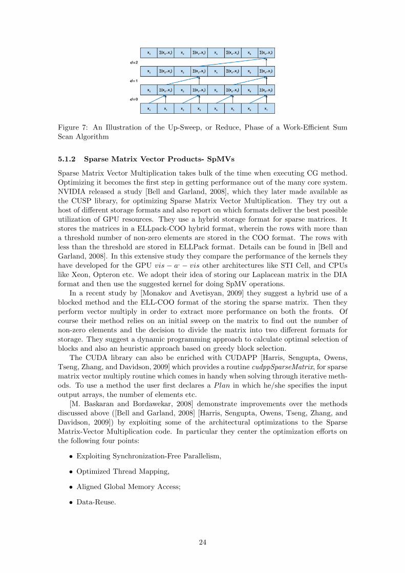
Figure 7: An Illustration of the Up-Sweep, or Reduce, Phase of a Work-Efficient SumScan Algorithm

5.1.2 Sparse Matrix Vector Products- SpMVs

Sparse Matrix Vector Multiplication takes bulk of the time when executing CG method.Optimizing it becomes the first step in getting performance out of the many core system.NVIDIA released a study [Bell and Garland, 2008], which they later made available asthe CUSP library, for optimizing Sparse Matrix Vector Multiplication. They try out ahost of different storage formats and also report on which formats deliver the best possibleutilization of GPU resources. They use a hybrid storage format for sparse matrices. Itstores the matrices in a ELLpack-COO hybrid format, wherein the rows with more thana threshold number of non-zero elements are stored in the COO format. The rows withless than the threshold are stored in ELLPack format. Details can be found in [Bell andGarland, 2008]. In this extensive study they compare the performance of the kernels theyhave developed for the GPU vis − a, − vis other architectures like STI Cell, and CPUslike Xeon, Opteron etc. We adopt their idea of storing our Laplacean matrix in the DIAformat and then use the suggested kernel for doing SpMV operations.

In a recent study by [Monakov and Avetisyan, 2009] they suggest a hybrid use of ablocked method and the ELL-COO format of the storing the sparse matrix. Then theyperform vector multiply in order to extract more performance on both the fronts. Ofcourse their method relies on an initial sweep on the matrix to find out the number ofnon-zero elements and the decision to divide the matrix into two different formats forstorage. They suggest a dynamic programming approach to calculate optimal selection ofblocks and also an heuristic approach based on greedy block selection.

The CUDA library can also be enriched with CUDAPP [Harris, Sengupta, Owens,Tseng, Zhang, and Davidson, 2009] which provides a routine cudppSparseMatrix, for sparsematrix vector multiply routine which comes in handy when solving through iterative meth-ods. To use a method the user first declares a Plan in which he/she specifies the inputoutput arrays, the number of elements etc.

[M. Baskaran and Bordawekar, 2008] demonstrate improvements over the methodsdiscussed above ([Bell and Garland, 2008] [Harris, Sengupta, Owens, Tseng, Zhang, andDavidson, 2009]) by exploiting some of the architectural optimizations to the SparseMatrix-Vector Multiplication code. In particular they center the optimization efforts onthe following four points:

• Exploiting Synchronization-Free Parallelism,

• Optimized Thread Mapping,

• Aligned Global Memory Access;

• Data-Reuse.

24

5.2 Conjugate Gradient

[Georgescu and Okuda, 2007] discuss how conjugate gradient methods could be aligned tothe GPU architecture. They also discuss the problems with precision and implementingpreconditioners to accelerate convergence. In particular they state that for double precisioncalculations problems having condition numbers less than 105 may converge and give aspeed-up also. They however warn that above a threshold value of the condition numberthe Conjugate Gradient Method will not converge. This last observation relates to thelimited double precision performance available on the GPU.

[Buatois, Caumon, and Levy, 2009] discuss their findings on implementing single pre-cision iterative solvers on the GPU and show that for Jacobi preconditioning and a limitednumber of iterations the GPU is able to provide a solution of comparable accuracy butas the iterations increase the precision drops in comparison to the CPU. They use theConjugate Gradient method exploiting some of the techniques like register blocking, vec-torization and the Block Compressed Row storage(BCRS) to extract parallel performanceon the GPU.

They try to maximize the throughput for the memory transactions by using 4×4 blocksin the BCRS format. This format later proves beneficial for strip mining operations. Usingsuch an arrangement complemented with the vector data types available on the GPU (forexample float4 that allows storing 4 32-bit floats to be stored at one index). By makingarrays of such aggregate data types one can access data in chunks thereby saving addresscalculation. For e.g. in the case of a 4× 4 block storage as shown in Figure 8, an array of4 float4’s can be used and accessing all elements is possible with a single address that ofthe array.

Figure 8: Sum reduction on a Scalar architecture with shared Memory

Further they suggest that individual elements within an aggregate data type couldbe allocated to multiple threads and such a pattern could be followed among the otherelements of this 4 float4 element array. Thereby providing speedups in reduction opera-tions. An important finding that is indicated in their results is that reordering of the typeCuthill-McKee did not show any influence on the implementations they executed for theGPU and the CPU.

5.3 Preconditioning

Techniques that are basically dependent on the Sparse Matrix Vector Multiply discussedin previous sections have been suggested in literature for accelerating Preconditioning ofIterative Solvers like GMRES and Conjugate Gradient. [Wang, Klie, Parashar, and Sudan,2009] use an ILU Block Preconditioner, which has poor convergence qualities but is easier

25

to parallelize, for solving a sparse linear system by the GMRES method. Coefficient matrix

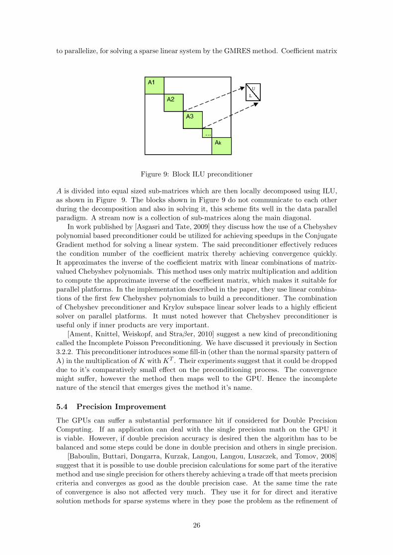
Figure 9: Block ILU preconditioner

A is divided into equal sized sub-matrices which are then locally decomposed using ILU,as shown in Figure 9. The blocks shown in Figure 9 do not communicate to each otherduring the decomposition and also in solving it, this scheme fits well in the data parallelparadigm. A stream now is a collection of sub-matrices along the main diagonal.

In work published by [Asgasri and Tate, 2009] they discuss how the use of a Chebyshevpolynomial based preconditioner could be utilized for achieving speedups in the ConjugateGradient method for solving a linear system. The said preconditioner effectively reducesthe condition number of the coefficient matrix thereby achieving convergence quickly.It approximates the inverse of the coefficient matrix with linear combinations of matrix-valued Chebyshev polynomials. This method uses only matrix multiplication and additionto compute the approximate inverse of the coefficient matrix, which makes it suitable forparallel platforms. In the implementation described in the paper, they use linear combina-tions of the first few Chebyshev polynomials to build a preconditioner. The combinationof Chebyshev preconditioner and Krylov subspace linear solver leads to a highly efficientsolver on parallel platforms. It must noted however that Chebyshev preconditioner isuseful only if inner products are very important.

[Ament, Knittel, Weiskopf, and Straβer, 2010] suggest a new kind of preconditioningcalled the Incomplete Poisson Preconditioning. We have discussed it previously in Section3.2.2. This preconditioner introduces some fill-in (other than the normal sparsity pattern ofA) in the multiplication of K with KT . Their experiments suggest that it could be droppeddue to it’s comparatively small effect on the preconditioning process. The convergencemight suffer, however the method then maps well to the GPU. Hence the incompletenature of the stencil that emerges gives the method it’s name.

5.4 Precision Improvement

The GPUs can suffer a substantial performance hit if considered for Double PrecisionComputing. If an application can deal with the single precision math on the GPU itis viable. However, if double precision accuracy is desired then the algorithm has to bebalanced and some steps could be done in double precision and others in single precision.

[Baboulin, Buttari, Dongarra, Kurzak, Langou, Langou, Luszczek, and Tomov, 2008]suggest that it is possible to use double precision calculations for some part of the iterativemethod and use single precision for others thereby achieving a trade off that meets precisioncriteria and converges as good as the double precision case. At the same time the rateof convergence is also not affected very much. They use it for for direct and iterativesolution methods for sparse systems where in they pose the problem as the refinement of

26

the solution xi+1 which can be written as:

xi+1 = xi +M(b−Axi), (98)

where M is the preconditioner and approximates S−1. If we use right preconditioningthen the system Ax = b reduces to the following

AMu = b, (99)

x = Mu (100)

Further they suggest calculating M using an iterative method and for the solution of theoriginal system a Krylov Subspace method is employed. This system of Inner and OuterIteration is now ready for Mixed Precision use. The idea here is that a single precisionarithmetic matrix-vector product is used as a fast approximation of the double precisionoperator in the inner iterative solver. They have reported the results for a non-symmetricsolver wherein the outer iteration is of a FMGRES and the inner one is a GMRES cycle.

5.5 Other Important Approaches

It is also possible to use multiple GPUs to boost the performance of an application. Mul-tiple GPUs stacked through the NVIDIA SLI interface or across workstations can collabo-rate via MPI. [Ament, Knittel, Weiskopf, and Straβer, 2010] use a redundant buffer basedscheme coupled with the availability of overlapping computation with memory transfersthrough the use of streams on the GPU. They divide the 3-D domains into tiles andeach GPU handles a subset of the tiles. This necessitates the inter-GPU communicationwhen the boundary layers are being updated in an iteration. They use synchronizationprimitives available on the GPU and the CPU for handling boundary cases.

6 Implementation

For our experiments we use a single core of a quad core Intel CPU (Q9650) running at 3.0GHz and having 12 Mb of L2 cache. The GPU we use is a Tesla machine with 30 StreamingMulti-Processors running at 1.3 GHz and a memory bandwidth of 102 GB/sec. We firstwrote the the Deflated Preconditioned CG Method on the host(CPU). An importantconsideration while writing the code was to make it modular so that it could be analyzedand optimized step-by-step. For this the following points were kept in mind.

1. Identifying Kernels of Computation.

2. Organizing code in form of kernels.

3. Prioritized Optimization of Kernels after subjecting the code to the profiler.

On the CPU we have used the Meschach BLAS Library for Dot Products and Saxpys.The kernels that were hand-coded are

1. Sparse Matrix Vector Multiply Kernel

2. Preconditioning Kernel(s)

3. Deflation Kernels

We (primarily) ran the kernels on grid sizes with 16000 to 260, 000 unknowns. Alsowe subjected these to Block sizes varying from 256 to 4, 096 unknowns per block. As afinal step deflation vectors were varied between 256 and 4, 096 as well. After the resultswere in line with the expectations which means

27

1. No. of Iterations decrease with Block-IC Preconditioning compared to plain Conju-gate Gradient,

2. With increasing block sizes the number of Iterations decrease further, and

3. With increasing number of deflation vectors number of iterations further decrease.

We proceeded with implementing the algorithm on the GPU. On the GPU the CUBLASlibrary provided some useful functions for saxpy, dot products which we have used.

6.1 SpMV Kernel

Our matrix has a regular pattern that of a 5-point Laplacean Matrix in two dimensions.So there are 5 diagonals which carry the complete matrix. It is important to mention herethat the matrix represents a grid n× n in size and hence the matrix has N = n× n rows.The storage format that we choose is called the Diagonal Storage format. All the diagonalsare stored in a 1-D array, starting from the lowest sub-diagonal(with offset −n) followedby sub-diagonal with offset (-1), then the main diagonal and then the two super-diagonalswith positive offsets. Also an important feature is that they all have the same length.This kind of uniformity of size makes coalesced access possible. So for example, if say thesub-diagonal with offset −1 has one element less, then at that position a zero fills in tomake it equal in size to the main diagonal.

Once stored in this way for each row of the matrix we have 5 fetches from the arrayholding the 5 diagonals and 5 from the vector. On the GPU we assign one thread tocompute one element of the resulting Matrix-Vector Product. Additional optimizationsinclude using shared memory and texture memory. The offsets array is accessed byevery thread and hence we store it on the shared memory to optimize the SpMV Kernel.This gives a very coalesced access pattern since threads in a half warp access contiguouselements in the array albeit each of those 5 accesses(per thread) are at offsets of n elements.

6.2 Preconditioning Kernel

The preconditioning kernel is the most sequential part of the entire algorithm. We ini-tially begin with the Block Incomplete Cholesky Preconditioning. The Block Variant ofIncomplete Cholesky Preconditioning basically exposes the parallelism at the block level.However each block has considerable serial amount of work to be done. This includesfetching three times block size number of elements from the array holding the precon-ditioner (this array is stored in a similar fashion as the coefficient matrix A) and alsofetching block size number of elements from the right-hand side vector. The computationper block is completely serial. A subsequent row needs a value from the previous row.

One technique that we have employed is to break down the steps of preconditioninginto three.

1. Forward Substitution

2. Diagonal Scaling.

3. Back Substitution

The second step of diagonal scaling can be heavily optimized using shared memory. Thisis possible since it is inherently parallel with two reads every thread followed by onemultiplication and all the calculations(N) are independent. For the first and the finalsteps we can also use shared memory. The trick is to load the elements using a numberof threads(number same as the block size) in parallel and then work on them and store

28

them back in global memory. Later in the development process we used Incomplete PoissonPreconditioning to maximize benefits of parallelism. It has been discussed earlier in Section3.2.2.

6.3 Deflation Kernels

For deflation we sub-divide the tasks into a couple of kernels at the outset. Namely,

1. Calculate b = ZTx

2. Calculate Matrix-Vector Product of E−1 with b.

3. Calculate Matrix-Vector Product of AZ with the result of the previous step andsubtract from x.

For the first kernel b = ZTx we have used the parallel sum approach. For the othertwo kernels it is useful to tailor the matrix multiplication example and use shared memoryinstead. This is better than the cublasSegmv(for some grid sizes) since we do not havean additional vector scaling and addition as required by cublasSgemv.

The decision to calculate E−1 explicitly is instrumental since it greatly reduces the timefor the iterations. Though the setup time for the algorithm is affected but the overall gainin the running time of the method more than compensate the costly operation. Althoughit is not sparse and we understand that if the number of deflation vectors become veryhigh then this approach might not be very efficient.

For the calculation of AZ× result of E−1 × b we used the cublasSgemv call. Thefinal calculation xit = Qb + P Tx can also utilize the kernels discussed here and also thecublasSgemv. In the later stages of development we optimize the storage of AZ andre-write the kernels for calculations involving AZ.

7 Optimizations and Results

In this section we list the data resulting from the experiments conducted. We start withsimple Conjugate Gradient Method and successively add Preconditioning and Deflationto it. First we present results from preliminary versions with minimal to no optimizationspresent. Further we apply optimizations and discuss the approaches. In all the resultsbelow we work with a Poisson type Matrix with a 5-point Laplacean stencil. Hence it has5 diagonals and is a regular sparse matrix.

7.1 Conjugate Gradient - Vanilla Version

As a first step we have implemented Conjugate Gradient(CG) on the CPU as well as on theGPU. For the GPU we only have one kernel, namely, the Sparse Matrix Vector ProductKernel. On the host side also we use a similar kernel. Albeit, it runs serially for all rowsone by one. We now provide a brief Code Commentary that outlines our code design.

7.1.1 Code Commentary

We use the Conjugate Gradient iteration as discussed in Algorithm 5. The convergencecondition being that the 2 − norm of the residual at the k−th step with respect to theoriginal residual r0 is minimized to a tolerance ε or less.

‖ rk ‖2‖ r0 ‖2

≤ ε. (101)

29

For the the CG code we have kept the tolerance at 10−6. The matrix A is kept in theform of diagonals and another matrix named offsets notes the offsets of these diagonalsfrom the main diagonal. Since for a 5−point Laplacean in 2−D we have 5 diagonals andit is symmetric. So the offsets are −n,−1, 0, 1, n where grid is n×n and the offset for maindiagonal is 0. Even though it is intuitive to use 3 diagonals for storage we use 5 since thatmakes the code simpler and on the GPU there is an added advantage of coalesced accessthat such a storage pattern provides.

As previously discussed the diagonals are of the same length N = n × n which is thenumber of unknowns for an n×n grid. This is useful when accessing these elements in theGPU since then each thread picks one element from each of the arrays and the memoryaccess becomes regular. This is explained in a simple example in [Bell and Garland, 2008].

The host code utilizes the Meschach library. It is an optimized BLAS library. Thereason we chose Meschach lies more in ease of use than anything else. An implementationof a more known library like gotoBLAS could be also interesting to compare. Anotheroption is to use Intel’s MKL library. All these Libraries provide functions for Dot Products,Saxpy, scaling and norm operations.

Sparse Matrix-Vector Products were done by summing up the product of elements ofeach row(of the matrix) with the corresponding vector element. This was repeated for allrows of the array inside a for loop.

For the GPU we mostly used CUBLAS as provided by NV IDIA. The dot productwas implemented using the cublasSdot and the saxpy similarly using cublasSaxpy. Alsouseful were the cublasScal for doing scaling and cublasSnrm2 for calculation of 2−norm.We developed three different flavors(versions) for Sparse Matrix Vector Product Kernelson the GPU

1. Vectorization - we simply copied the kernel from the Host and removed the for loop.Instead now each row is calculated by a separate thread.

2. Vectorization with the offsets array stored in the Shared Memory.

3. Vectorization with the offsets array and x stored in the Shared Memory.

Putting the offsets array in shared memory gave us a significant performance boost.Since the offsets array is accessed by every element in every row so it was imperative toput it in shared memory.

Throughout the inner loop for CG (steps 2 to 8 of Algorithm 5) there is no transferof information between the host and the device (except for transferring results of dot-products from the GPU to the host). On basis of the parameter OPT THREADS theoptimum number of threads [usually 256 but can be 512 for bigger grid sizes ] are assignedfirst and the block size is calculated as N

OPT THREADS . If the block size is more than thatsupported by the device then the number of threads is increased and the number of blocksis updated accordingly.

We initially tested this implementation with three different storage formats(CSR,DIAand Matrix-Free). Details about the CSR and DIA format can be found in [Bell and Gar-land, 2008]. The matrix free format eliminates use of any matrices to store the coefficientarray A. Instead all operations on the matrix can be specifically coded. For e.g. for the5-point Laplacean matrix the diagonal matrix diag(A) is 4 repeated N times. Similarlyfor other diagonals similar rules can be defined and operations can be written without anystorage space for the matrix.

The DIA format gives us the best results in terms of speedup so we performed com-parison of the SpMV kernels on DIA format only. We chose the DIA structure to moveahead since CSR is not well suited for our kind of matrix and matrix-free is too specific.

30

As previously mentioned we have largely relied on CUBLAS and shared memory basedoptimizations. Although texture memory could be useful when an array is accessed in anunordered way we have not used it for x since x changes in our application. Texturememory could be useful for smaller sizes of A but since it cannot be useful for larger gridsizes we have not used it. We tried it both for storing the coefficient matrix A and thevector x in separate versions of the code.

7.1.2 Comparisons with GPU versions

In Figure 10 we show a comparison of the Conjugate Gradient Algorithm’s run time onthe Host and Device across three Grid sizes.

1. 128× 128, 16384 unknowns ( 16,000)

2. 256× 256, 65536 unknowns ( 65,000)

3. 512× 512, 262144 unknowns ( 260,000)

4. 1024× 1024, 1048576 unknowns ( 1,000,000)

5. 2048× 2048, 4194304 unknowns ( 4,000,000)

6. 4096× 4096, 16777216 unknowns ( 16,000,000)

Figure 10: Conjugate Gradient on Host vs Device

Before we delve into the result analysis it is important to talk about divergence onthe GPU. Divergence could be misleading as divergence of the CG method. Howeverdivergence in terms of CUDA means presence of an If − then − else construct. This

31

retards the throughput of the kernel since it forces all the threads in a block to first takethe if path and then take the else path. In our case, suppose each block has 256 threads.Now since the offset array has five entries in it −n,−1, 0, 1, n five threads are needed toload it in parallel. However the rest of the 251 threads have nothing to do which wastessome of the device time. This phenomena is termed as divergence on the GPU. The secondflavor of our tests as listed in 7.1.1 has this kind of divergence in it however the effectsof divergence are more than compensated by the reduction in repeated global memoryaccess.

Looking at the results in Figure 10, we get a speed-up of around 21 times (for thelargest grid size)for the shared memory kernel which only caches offsets. The version withthe vector x also in the shared memory comes a close second and that is because of thedivergence that such a design has. It has to access some elements of x from the sharedmemory and some from the global memory. So the advantage of shared memory is greatlyreduced. For this reason we choose the variant of SpMV kernel that only utilizes sharedmemory for storing offsets only.

It must be noted that here for sizes greater than 260k we haven’t run the method uptill convergence as the code stops at 1000 iterations.

7.1.3 Profiler Picture

The SpMV kernel takes the maximum amount of time for the execution as far as GPUexecution is concerned. The shared memory tweak of loading the offsets though hasdivergence but it reduces the amount of GPU time SpMV kernel takes by half. In Figure11 and Figure 12 this can be observed. It can also be seen that as the number of unknownsincreases, more and more time is consumed by these three kernels of SpMV, saxpy andsdot.

Figure 11: Conjugate Gradient with basickernel

Figure 12: Conjugate Gradient with sharedmemory kernel

From Figure 10 it can be seen that at the size of 16M the speedup seems to becomeconstant. The reason for this is that the kernels on the GPU become bandwidth-bound.The CUBLAS calls are taking around 85Gb/s of the available bandwidth. The onlyhand-written kernel of SpMV is consuming more than 85 Gb/s. This kernel is at 100%occupancy. The rest of the calls are to CUBLAS functions and they are also at 100%occupancy.

32

7.2 Diagonal Preconditioning

Since our matrix for now is a simple 5-point Laplacean matrix (with similar elementson the diagonal) we did not expect any changes and our results stayed the same. Thepreconditioner step only involved scaling the main diagonal by 1

4 which was rather trivialto implement using a cublasSscal call. On the host-side this is implemented by a scalar-vector multiplication routine.

7.3 Conjugate Gradient with Preconditioning

7.3.1 Code Commentary

Extending CG with the Incomplete Cholesky Factorization based preconditioning is thenext step in our implementation. For this another kernel comes in place for the operation

zj = M−1rj (102)

where,

M = KKT (103)

and K is the (incomplete) lower Cholesky triangle. In order to keep it ”incomplete”K follows the sparsity pattern of A. We solve the system KKT zj = rj in three steps inthe following way:

1. Ky = rj Forward Substitution

2. y = y ∗ diag(K) Diagonal Scaling

3. KT zj = y Back Substitution

This step occurs inside the iteration as well, as shown on line number 6 of the Precon-ditioned Conjugate Gradient Iteration listing in Algorithm 7.

It must be noted that block sizes are always at least double the number of grid pointsin one direction. This is important since if they are between the grid dimension in say,the X direction, and 2× that size then they do not really suit the GPU (multiples of 32,16 only suit) and if they are less than the grid size in any one dimension they completelyremove the outer most diagonals in A. Recalling that A resembles the 5-point Laplaceanin cases of our interest. This is better explained by a picture given in the Appendix B.2.

We have followed these rules for the host also for a similar comparison. As can benoticed in Figure 13 preconditioning reduces the number of iterations required for con-vergence drastically. For grid sizes 4M and above the convergence does not occur within1000 iterations. However the norm of the result at the 1000th iteration decreases withbigger preconditioner block sizes. This can be observed in Figure 14

7.3.2 Comparisons with GPU versions

Comparing the CPU version of the code in Figure 15 to 20 with the GPU versions wesee that for smaller grid sizes the GPU version lags behind the CPU. However some gainis induced for bigger grid sizes. This could be partly explained by the relatively largeblock sizes which might become overwhelming for the closest (and the fastest) level ofcache inside the CPU. Also from these figures we can see that as the block sizes increase(and number of blocks decrease) the CPU gains a bit and this is because the number ofiterations in the for loop is less, so less jumps in the CPU code hence better performance.

The most simple version of the kernel code for preconditioning would have been puttingall the three steps (forward substitution, diagonal scaling and backward substitution) in

33

Figure 13: Decreasing iterations across block sizes (CG with Block-IC Preconditioning)

Figure 14: Norm decreasing with decrease in number of blocks (CG with Block-IC Pre-conditioning)

34

one kernel but that takes up a lot of registers. So we broke them down in three parts. Outof these three parts diagonal scaling is embarrassingly parallel so it consumes less than1% of the total time required for preconditioning but forward substitution and backwardsubstitution are inherently sequential and not suited for the GPU. However computingthem on the CPU every cycle and then transferring back and forth between the GPU-CPU is not a good solution either.

Hence as much as Block-IC permits we used shared memory for temporary calculationof the new values in each block and once the calculations are complete we copy them tothe global memory. This means that for each block of the Block-IC method we store ’sizeof block’ number of floats in which we store the result y = K−1rj for the back substitutionand the forward substitution steps. This seems natural since in the implementation offorward and back substitution y is written at most three times in the whole iteration thatspans across a block, so keeping it in shared memory and writing only the final valueimproves performance.

As promising as this approach sounds it fails as soon as block sizes approach 4096which happens for a grid size 1024×1024 in our experiments. Then we have to come backto the naive kernel that launches one thread per block that calculates the new vector perblock.

This approach also might loose on bigger grid sizes (if and when we have that muchshared memory) since then a lot of copying will have to be done by a single thread fromshared memory to global memory.

We also tried using as many threads in a block as there were elements in the block andtried to load all elements in parallel and store them back in parallel but the intermediatestep of calculating all elements of y was done by a single thread. This version also fails forthe same reason as the previous approach does. There can be a maximum of 512 threadsper block so beyond that it is not possible to use this idea of co-operative loading andwriting back.

An even more aggressive version (using shared memory) for the forward and backsubstitution steps is to store the matrix K’s three diagonals also in shared memory, thoughit becomes unusable even faster than the previous approach.

Preconditioning of the Block-Incomplete Cholesky type is best when there are moreand more blocks that can all be computed in parallel. However as the block sizes increasethe amount of the time that GPU is under-utilized also increases. Since inside the for-ward/back substitution kernels only one thread works per block which is wasteful for theGPU.

Figure 15 to 20 show how how speedup slowly crawls up to 2.5 times from a fractionallevel for large grid sizes. In these graphs the blue color shows the kernel in which sharedmemory can be used for storing the intermediate result y and the green color shows thenaive kernel which has to be used after a certain point since shared memory is limited to16384 bytes or 4096 single precision floats per block.

7.3.3 Profiler Picture

Preconditioning dominates more than 90% of the execution time (across all grid sizes andpreconditioning block sizes) in on the device versions of the code. This was expectedbecause of the serial nature of the code. Saxpy, Sdot and SpMV come a close second. Onthe host the majority of the time is taken up by the SpMV operation and the Block-ICPreconditoning.

On the host this percentage rises much more slowly as compared to the device. Sincefor the device(GPU) serial code is not suited at all.

35

Figure 15: SpeedUp across block sizes for16k unknowns

Figure 16: SpeedUp across block sizes for65k unknowns

Figure 17: SpeedUp across block sizes for260k unknowns

Figure 18: SpeedUp across block sizes for 1Munknowns

7.4 Conjugate Gradient with Deflation and Preconditioning-Block IC

Deflation is applied to the existing preconditioned iteration. Deflation provides muchmore scope for exploiting parallelism and that will be evident with the results discussedhenceforth. First we put the optimized kernels on the device, then we added change theway we calculate and store AZ. While improving the performance of the code on the GPUwe also gave equal attention to optimization of the CPU code.

7.4.1 Code Commentary

We implemented deflation on the Block Incomplete Cholesky version of the code discussedin the previous section. Sub-domains were introduced in the grid which could be handledby separate processors. The Sub-domains have been assigned stripe-wise (for details referAppendix B.4) so that in the matrix a set of rows (one domain) could be assigned to oneprocessor. The new operations required for Deflated Preconditioned Conjugate Gradientcan be written down in separate kernels.

1. Calculation of AZ (happens once).

2. Calculation of E (happens once).

3. Calculation of E−1 from E (happens once).

4. Calculation of m = ZTx (happens every iteration).

36

Figure 19: SpeedUp across block sizes for 2Munknowns

Figure 20: SpeedUp across block sizes for 4Munknowns

5. Calculation of y = E−1m (happens every iteration).

6. Calculation of result= x−AZy (happens every iteration).

7. Final Update of x, the solution with Qb and P Tx (happens once).

Now AZ, E−1 can be calculated on the CPU itself. Since the setup of the kernel isnot included in our analysis of speedups. This part is common to both the host and thedevice kernels.

After we have calculated E−1 the 5th step in the list above is a Dense Matrix VectorMultiplication. Similarly the 6th step also since we store AZ as a full matrix of dimensionsN × d where N is the number of unknowns (also N = n × n, where n is grid size in onedimension) and d is the number of deflation vectors.

This limits our experiments to a grid size of a maximum of 512×512 with 4096 domainssince at this size AZ alone requires 4 gigabytes of storage which is a limit for the GPUwhich has only 4GB of Global Memory storage. In order to overcome this limitation, laterwe store AZ in a format where only 5×N storage is required.

For doing Dense Matrix Vector Multiplication we use the CublasSgemv function. Forthe 4th step, ZTx, we write a simple kernel that sums up N/d elements in each thread.

For the final step which involves correcting the solution x. We have to do AZTx whichcan again be computed using a CublasSgemv call. Also we have to calculate E−1AZTxand E−1ZT b.

7.4.2 Comparisons with GPU versions

Figure 21 to 23 present the speedup on three different grid sizes and across three differentnumbers of deflation vectors and three different numbers of preconditioning blocks.

Detailed results with Error norms for device and host and the number of iterations areavailable in the Appendix C.1.1. A couple of things are worth noting in these results.

• The number of iterations decrease with increasing block size for any number ofdeflation vectors.

• Increasing the number of deflation vectors decreases the number iterations requiredfor convergence.

• The relative error norm is same across the device and the host

37

Figure 21: Deflated Block-IC Preconditioned Conjugate Gradient (Simple CUDA kernel)16k unknowns

Figure 22: Deflated Block-IC Preconditioned Conjugate Gradient (Simple CUDA kernel)65k unknowns

Figure 23: Deflated Block-IC Preconditioned Conjugate Gradient (Simple CUDA kernel)260k unknowns

38

• The Speed-Up is maximum for the largest number of deflation vectors and the small-est Block Size (largest number of blocks).

The first three observations confirm that the results are correct. The last observationconfirms that as the parallelism increases in the code the usefulness of the GPU appearsin the execution times. They are reduced considerably.

However there is one interesting thing to be noted in the speedups for the grid size512 × 512 (Figure 23). The maximum speedup is for the number of blocks at 128 andwhen the number of blocks increases to 256 the speedup declines.

This has something to do with the hardware we have. We use a Tesla C1060 GPU with240 scalar processors. They are divided amongst 30 Multiprocessors in groups of 8.Thepreconditioning kernel we use now is the naive kernel, in which the Forward and BackwardSubstitution kernels form the bulk of the computing time. This remains true for deflatedPreconditioned Conjugate Gradient as well as we will discuss in the Profiler Picture sectionthat follows. These kernels (forward and backward substitution) launch as many CUDAblocks (CUDABLOX from hereon for clarity’s sake) as there are preconditioning blocks.So 128 CUDABLOX are launched when there are 128 preconditioning blocks. Now in thiscase we have enough scalar processors to process all of these blocks simultaneously. Sinceonly one thread calculates the whole preconditioning block in both kernels.

However in case of the 256 blocks we have a limitation that first 240 blocks will bescheduled and then once they are done the remaining 16 blocks are scheduled. This canalso be verified from the execution times for this particular case. As can be seen in Figure24 and 25, the execution times rise only on the GPU whereas across block sizes 64 and128 they are more or less constant. The occupancy in both cases is the same and thebandwidth is more (50%) for the case when the number of blocks is 128. This couldn’t becompared in the previous version of the code (Section 7.3) since there we had two differentkernels for different block sizes.

7.4.3 Profiler Picture

At this stage we have 24 (3 grid sizes, 3 preconditioning block sizes, 3 different deflationvector counts (2 for the last grid size)) different instances of the solution we are tryingto implement so we only display a couple of profiler pictures that make the point clear.Specifically we discuss the case from the 128×128 matrix for 1024 deflation vectors acrossall preconditioning block sizes and for the grid size 512× 512 we do the same.

From Figure 24 we can infer that the calculation of AZ × x is crucial at all precon-ditioning block sizes however its contribution is shadowed by the preconditioning kernels(forward substitution and back substitution) as the preconditioning block sizes increasesor the number of preconditioning blocks decreases. This is because each thread on theGPU (which calculates one complete block) has to work more and more.

Careful examination of figure 25 , which is for grid size 512×512, we can see that fromthe number of blocks 128 and 256 there is a slight increase in the preconditioning timewhich accounts for the decrease in speedup as shown in the earlier in Section 7.4.2.

7.5 Conjugate Gradient with Deflation and Preconditioning - AZ stor-age optimized

As seen in the previous two sections the CublasSegmv call for calculating AZ × x is thesecond most time consuming kernel after preconditioning (considering forward and backsubstitution as one and ignoring the diagonal scaling step since it is inherently parallel).Keeping the preconditioner same we try to optimize this kernel.

39

!!

Figure 24: Conjugate Gradient with Deflation and Block-IC Preconditioning (Simple Ver-sion) Deflation Vectors=1024

!! !

Figure 25: Conjugate Gradient with Deflation and Block-IC Preconditioning (Simple Ver-sion) Deflation Vectors=1024

40

Figure 26: 5 diagonals in AZ. N=64, n=8 and d=16

The reason why this kernel is taking so much time is the order of computations involved.AZ is an N × d matrix to which a vector of size N is multiplied in this kernel. Now weexamine the structure of AZ in Figure 26.

The blue areas form the diagonals with offsets ±d/n and width N/d per column. Themain diagonal is also N/d wide per column. The green areas form the diagonals withoffsets ±1. So the blue areas have in all N − n elements. The red area has N elementssince N/d× d = N . The green area has d− 1 elements on each side of the main diagonal.

Now to make the storage structure uniform we use a block of 5 ∗ N elements. Outof which one chunk of N is assigned to the main diagonal. The diagonals (in blue) withoffset ±d/n can be stored in chunks of N each with padding of zeros before(−n/d) orafter(+n/d). For the green areas, i.e. the diagonals with offset ±1, there is paddingrequired at every element which is a zeros pattern N/d long. This way all diagonals canoccupy N spaces and the data structure can now be used. One of the main reasons, otherthan saving space, for storing AZ like this is also that such an arrangement makes it very

41

!"

# !"

#

$%&$$$'

( %&$$$'

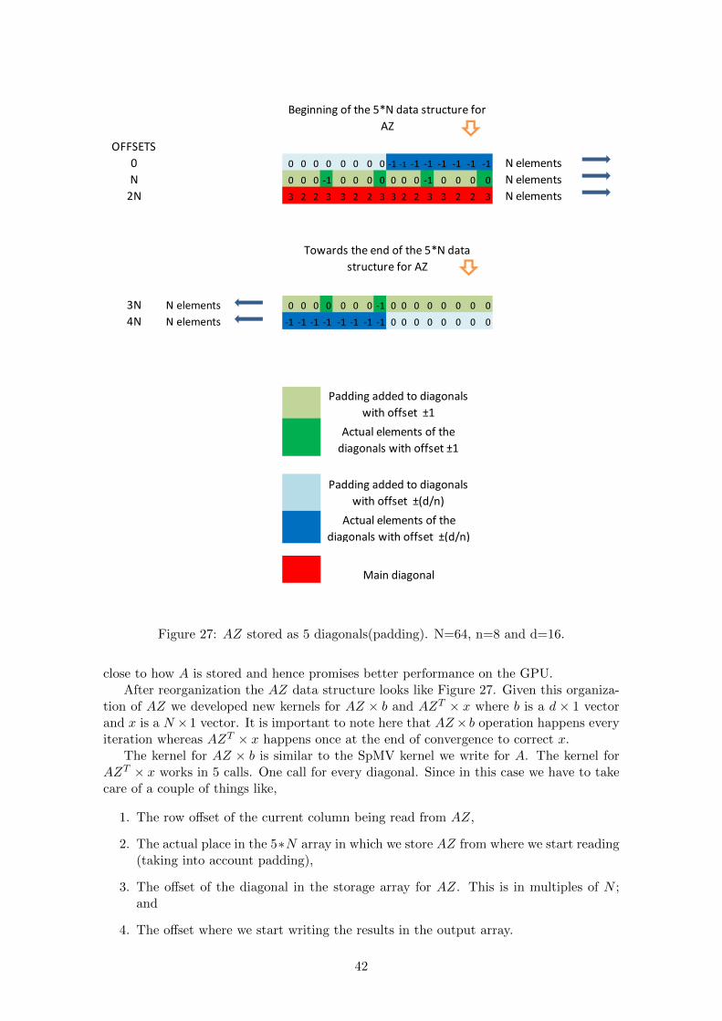
Figure 27: AZ stored as 5 diagonals(padding). N=64, n=8 and d=16.

close to how A is stored and hence promises better performance on the GPU.After reorganization the AZ data structure looks like Figure 27. Given this organiza-

tion of AZ we developed new kernels for AZ × b and AZT × x where b is a d × 1 vectorand x is a N ×1 vector. It is important to note here that AZ× b operation happens everyiteration whereas AZT × x happens once at the end of convergence to correct x.

The kernel for AZ × b is similar to the SpMV kernel we write for A. The kernel forAZT × x works in 5 calls. One call for every diagonal. Since in this case we have to takecare of a couple of things like,

1. The row offset of the current column being read from AZ,

2. The actual place in the 5∗N array in which we store AZ from where we start reading(taking into account padding),

3. The offset of the diagonal in the storage array for AZ. This is in multiples of N ;and

4. The offset where we start writing the results in the output array.

42

!

Figure 28: Deflated Conjugate Gradient with Block-IC Preconditioning. 128× 128 grid.

!

Figure 29: Deflated Conjugate Gradient with Block-IC Preconditioning. 256× 256 grid.

The kernels after re-organization of AZ have been written for the host side as well.We now show the comparisons of the two codes running on the host and the device.

7.5.1 Comparisons with GPU versions

With the optimized storage of AZ we reduce the effective number of multiplications byaround two orders of magnitude or more. This is a mixed blessing for the GPU version ofthe code since previously (when we had full AZ) more calculations meant more parallelism,but now that reduces and furthermore due to the smaller size of the AZ matrix it fits betterin the CPU memory (cache). Result being that the GPU gains in speed by 2x whereasthe CPU gains 20x. Effectively the speedups are decimated. Figure 28 to 30 show thiseffect.

7.5.2 Profiler Picture

Since we have optimized one of the heavyweights from the previous version of the code asin Section 7.5. Now the majority of the time is spent in preconditioning and as the gridsize increases preconditioning dominates more and more.

This is visible in Figure 31 to 33. In the following section we will try to address the

43

!

Figure 30: Deflated Conjugate Gradient with Block-IC Preconditioning. 512× 512 grid.

Figure 31: Deflated Preconditioned Conjugate Gradient(AZ storage optimized). Grid Size(128× 128)

Figure 32: Deflated Preconditioned Conjugate Gradient(AZ storage optimized). Grid Size(256× 256)

44

Figure 33: Deflated Preconditioned Conjugate Gradient(AZ storage optimized). Grid Size(512× 512)

problem with sequential nature of Block-IC preconditioning with a new kind of Precondi-tioning that gives ample scope for parallelism.

7.6 Conjugate Gradient with Deflation and IP Preconditioning - AZstorage optimized

After optimizing AZ storage most of the time is spent in the preconditioning kernels,namely the forward and back substitution steps. In order to get a better speedup weexperimented with the IP preconditioning (discussed in Section 3.2.2) approach suggestedby [Ament, Knittel, Weiskopf, and Straβer, 2010].

This preconditioner is inherently parallel since it( M−1) is also composed of 5 diag-onals. In order to calculate the updated vector y we need to do a sparse matrix vectormultiplication just like we do for Ax. This dramatically affects the run time of the algo-rithm as we show below in the results.

7.6.1 Comparisons with GPU versions

We made a CPU version for Deflated IP Preconditioned CG with optimizations to AZand compared it with an equivalent GPU version written in CUDA. After optimizing thepreconditioning we again get upto an order of magnitude speedups. See Figure 34.

It is also useful to put into perspective the speedups we had with the previous versionthat used Block-IC Preconditioning.

From Figure 35 to 37 we can see the improvement in speedup that IP Preconditioningoffers for our problem. Also it is important to compare the number of iterations taken inthe Block-IC variants for convergence to those required for the Incomplete Poisson versionto converge. In Figure 38, 40 and 42 we can see that we pay a small cost for the parallelismby having a slightly higher iteration count for IP Preconditioning based solution comparedto the highest number of blocks based Block-IC Solution.

Finally if we compare the error norms (Figure 39, 41 and 43) of the solution for allthe cases, they are also comparable between all variants of Block-IC based DPCG and IPbased DPCG.

45

Figure 34: Deflated Preconditioned Conjugate Gradient with IP Preconditioning acrossthree grid sizes

Figure 35: Grid Size 128× 128

Figure 36: Grid Size 256× 256

46

Figure 37: Grid Size 512× 512

7.6.2 Profiler Picture

Looking at the profiler output in Figure 44 to 46 now we see that it is dominated by the thecublasSgemv call for the operation E−1b. for larger number of deflation vectors. Howeverat smaller number of deflation vectors the execution time is almost evenly distributed.

The important thing that emerges out of these figures is that the kernel for E−1b mustbe optimized since it is taking the majority of the time. For smaller number of deflationvectors however the percentage of time taken for E−1b comes down due to a decreasein the number of operations involved and the dot product kernels also take a significantamount of time.

7.7 Conjugate Gradient with Deflation and IP Preconditioning - AZstorage optimized and optimized Matrix Vector ( E−1b) Multiplica-tion

After optimizing storage of AZ and preconditioning the dominant part of the kernel be-comes the the matrix vector product E−1b as shown in the results in the Profiler Pictureof previous section 7.6.2. As previously (Section 6.3) discussed this method (of calculatingE−1 explicitly) was chosen for its suitability for the GPU since it could be otherwise becalculated using the substitution methods which are completely serial.

For optimizing this operation better than with CUBLAS (cublasSgemv) we use theMagma Library for CUDA version 0.2. The memory throughput of the Magma gemvfunction is much better than cublasSgemv. It often (for many matrix sizes) is 2.5 timesfaster than CUBLAS.

In addition to this major change we also club some of the existing functions thatinvolved saxpys and copy/scaling operations on the device involving α and β for calculatingthe new search direction and updating the residual vector(see steps 4 and 7 of Algorithm5). These deliver close to 8 − 9% improvement over all the grid sizes in addition to theimprovment due to the use of MAGMA.

7.7.1 Comparisons with GPU versions

In Figure 47 to 49 we present the results of using the the blas routine gemv from theMAGMA library. As one can notice the effect is significant when compared to the pre-vious best version we have that of Incomplete Poisson Preconditioning (with AZ storage

47

Figure 38: Grid Size (128× 128)

Figure 39: Grid Size (128× 128)

Figure 40: Grid Size (256× 256)

Figure 41: Grid Size (256× 256)

Figure 42: Grid Size (512× 512)

Figure 43: Grid Size (512× 512)

48

Figure 44: Deflated IP Preconditioned Conjugate Gradient. Grid Size (128× 128)

Figure 45: Deflated IP Preconditioned Conjugate Gradient. Grid Size(256× 256)

49

Figure 46: Deflated IP Preconditioned Conjugate Gradient. Grid Size(512× 512)

optimized) and CUBLAS. In some cases the speedup has also doubled. The host versionhas been kept the same as was in the previous (Section 7.6) experiment.

7.7.2 Profiler Picture

The MAGMA blas library has levelled the execution times to a large extent. In the Figure50 through 52 it can be noticed that the E−1b operation execution time now scales withthe number of deflation vectors almost linearly. Also worth noting is that for the biggestproblem size in the Figure 52 for a Grid Size of 512×512 and 4096 deflation vectors we getthe bandwidth for the gemv kernel at 86Gb/s which is substantial since Tesla hardwaresupports a maximum of 101 Gb/s of Memory Bandwidth.

8 Experiments with Two Phase Flow Matrix

Till now all the results we have shown had the 5-point Laplacean Matrix as the coefficientmatrix A. However the real intent of this study is to solve the multi-phase flow problems.By picturing two phases in the coefficient matrix we have a problem that is just a hairremoved from a potential multi-phase/bubbly flow problem.

All that changes are the coefficients in the matrix A. Its structure remains the same.However since we are picturing fluids with very different densities there is a significantdiscontinuity between the coefficients now. As discussed in Section 2.1 we work with amatrix of the same structure, however with a very different condition number. The twophase flow matrix in its original form is not invertible. That is a problem if we want tofind a solution to Ax = b. We force invertibility by setting A(N,N) = 2, where N = n×nand n =grid size in one dimension.

8.1 Conjugate Gradient -Vanilla Version and with Block- IC and Diag-onal Preconditioning

We ran Conjugate Gradient Algorithm with Block-IC Preconditioning (size of blocks =2 × n where N = n × n) and Diagonal Preconditioning and record the variation in the

50

Figure 47: Grid Size(128× 128)

Figure 48: Grid Size(256× 256)

51

Figure 49: Grid Size(512× 512)

Figure 50: Deflated (IP) Preconditioned Conjugate Gradient. (AZ storage optimized andMagma BLAS based gemv) Grid Size (128× 128)

52

Figure 51: Deflated (IP) Preconditioned Conjugate Gradient. (AZ storage optimized andMagma BLAS based gemv) Grid Size (256× 256)

Figure 52: Deflated Preconditioned Conjugate Gradient. (AZ storage optimized andMagma BLAS based gemv) Grid Size (512× 512)

53

error norm of the solution and the residual norm over multiple iterations (even afterthe convergence). What we notice is that the residual norm keeps on falling. This isnot correct at all since, if the norm starts from 102 and falls below 10−6 it is exceedingmachine precision for single-precison floating point operations and that is not possible.In the graphs that follow from Figure 53 to 57 for Conjugate Gradient with DiagonalPreconditioning and from Figure 58 to Figure 62 for Conjugate Gradient with Block-ICPreconditioning we see this phenomenon clearly. The thin vertical blue line in all thegraphs is where convergence is achieved. The solid blue line traces the norm of the errorin the solution and the red line is the norm of the residual. The precision criteria for thesetests was set to 10−5. They have have been run on smaller grids in order to show theeffect in lesser number of iterations. With larger grid sizes (those above 16384 unknowns)the behavior is similar. The green vertical line shows where machine precision is hit.

These two results prove that even though convergence happens and relative residualnorm reaches a value lower than the expected precision (10−5 in these calculations) itis a sort of false stop. The residual rises and falls some more times before it becomesmeaningless (seems to become better than machine precision) and the error norm of thesolution which is at a relatively higher value at the time of convergence also comes downafter the observed convergence. This is in line with the work previously done [Tang, 2008].

8.1.1 Comparisons with GPU versions

We first ran the Conjugate Gradient algorithm on the two phase matrix, followed by twoexperiments with Diagonal and then Block Incomplete Cholesky Preconditioning. Weget comparable speedups (Figure 63) to Section 7.1.2. However the norm (Figure 64) ofthe relative error in the solution remains high due to the ill-conditioning of the originalproblem.

For Block Incomplete Cholesky Version we have three different block sizes which re-sult in three different number of blocks. These are denoted by X DIREC

2 , X DIREC4 and

X DIREC8 . Here X DIREC denotes the dimension of the grid in x-direction. For our

experiments we have a square grid hence dimensions are n× n and number of unknownsN = n × n. Hence n = X DIREC. For e.g. if n = 256 then X DIREC = 256 andsubsequently we have Number of Blocks as 128, 64 and 32.

8.2 Conjugate Gradient with Deflation and Block-IC Preconditioning

In this section and the next one we summarize the speedups for Conjugate Gradient withDeflation and Preconditioning. Deflation takes toll on the precision condition we fix as10−6 for the previous tests (without deflation only preconditioning in section 8.1). Resultbeing that the precision condition has to be scaled down to 10−2 and then the methodseems to converge. For deflation we use the most optimized version that we have had fromthe previous results in Section 7.7.

We present the results for calculated norms on three grid sizes 128 × 128, 256 × 256and 512×512 across three different number of deflation vectors and preconditioning blocksizes in Figure 65. In these results the ratio of the densities of the two mediums is 10,unlike the previous experiments (Section 8.1) where it was 1000. As can be seen except forGrid Size 128 × 128 at number of deflation vectors = 1024 we have a peculiar case whenthe error norm rises and the solution is more erroneous than the initial guess. Otherwisethe error norm is a between 0 and 1.

More detailed results are available in the Appendix C.2.1. The reason for this behavioris the deteriorating condition number of A due to the two phase matrix. It is worsenedfor the Projection matrix P that has to be constructed for deflation.

54

Figure 53: Conjugate Gradient with Diag-onal Preconditioning for Two-Phase Matrix(Grid Size 8× 8)

Figure 54: Conjugate Gradient with Diag-onal Preconditioning for Two-Phase Matrix(Grid Size 16× 16)

Figure 55: Conjugate Gradient with Diag-onal Preconditioning for Two-Phase Matrix(Grid Size 32× 32)

Figure 56: Conjugate Gradient with Diag-onal Preconditioning for Two-Phase Matrix(Grid Size 64× 64)

Figure 57: Conjugate Gradient with Diag-onal Preconditioning for Two-Phase Matrix(Grid Size 128× 128)

55

Figure 58: Conjugate Gradient with Block-IC Preconditioning for Two-Phase Matrix(Grid Size 8× 8)

Figure 59: Conjugate Gradient with Block-IC Preconditioning for Two-Phase Matrix(Grid Size 16× 16)

Figure 60: Conjugate Gradient with Block-IC Preconditioning for Two-Phase Matrix(Grid Size 32× 32)

Figure 61: Conjugate Gradient with Block-IC Preconditioning for Two-Phase Matrix(Grid Size 64× 64)

Figure 62: Conjugate Gradient with Block-IC Preconditioning for Two-Phase Matrix(Grid Size 128× 128)

56

!"#$%&' !"#$%&' !"#$%&' $()*+(

Figure 63: Speedup across various sizes for different variants

!"#$%&' !"#$%&' !"#$%&' $()*+(

Figure 64: Relative Error Norm of the Solution ‖Xexact−Xk‖2‖Xexact‖2 across various sizes for dif-

ferent variants

57

!"#$#%

!"#$% &'%!" !"#$% &'%! !"#$% &'%! !""#$% &'%! !""#$% &'%! !""#$% &'%! !"#$% &'%! !"#$% &'%! !"#$% &'%!"

Figure 65: Two Phase Matrix with Density Contrast (10 : 1). Relative Error Norm of the

Solution, ‖Xexact−Xk‖2‖Xk‖2

58

Looking at the Speedup picture (Figure 66) we find that speedups closely resemble theresults in a previous section(7.5) with a simple 5-point Laplacean Matrix.

8.3 Conjugate Gradient with Deflation and IP Preconditioning

Following the setup of Section 8.2 we conduct the test runs for the IP Preconditioner caseand see slightly better speedups attributed to the parallel nature of the preconditioner(Figure 68). However the relative error norm of the solution at convergence is very high(comparable to values in Section 8.2).

We present the results for three grid sizes 128 × 128, 256 × 256 and 512 × 512 acrossthree different number of deflation vectors per grid size in Figure 67. In these results theratio of the densities of the two mediums is 100, unlike the previous experimentSection8.2) where it was 10 and 1000 in the first experiments Section 8.1.

The speedups (Figure 68) closely resemble the speedups from the Section 7.6.The profiler pictures don’t change much for sections 8.2 and 8.3 since only the matrix

changes and not the methods of computation. The kernel execution times follow similarpattern as that of the Poisson type Matrix (similar to Sections 7.5 and 7.6).

9 Analysis

In this section we look at the different aspects of our implementations. We try to findout how much parallelism we exploit and how much bandwidth we are able to utilizeon the GPU. We end this section with a discussion on what might be possibly limitingthe achievable speedup and how far we are from that point. Throughout this section weanalyze the results with a grid size of 512×512 and 4096 deflation vectors and IncompletePoisson Preconditioning. Specifically the results from Section 7.7 are used unless otherwisementioned.

9.1 Static Analysis

In this section we calculate how many Floating Point Operations (FLOPs) each kerneldoes in each run. Also we list out how many memory accesses happen both during loadand stores.

We list them for all the Kernels. In general a few variables can be defined.

• N, Number of Unknowns

• d, Number of Deflation Vectors

• m, Number of Iterations

• n, Grid Dimension

From Table 1 we can find out the number of Operations being performed in onecomplete run of the methods we have implemented.

We now elaborate some of the Kernel names:ZTx, E−1b and AZ × E−1b form the steps of the deflation operation. Forward Sub-

stitution, Diagonal Scaling and Back Substitution form the steps of Block IncompleteCholesky Preconditioning. Sdot is the Dot product function as named in BLAS libraries.We use cublasSdot. Saxpy is the Saxpy Kernel as available in BLAS libraries. We usecublasSaxpy and also write custom kernels to club saxpy with scaling operations to min-imize memory transfers. Sscal is the BLAS scaling operation and Snrm is the 2-Normoperation available in the BLAS libraries.

59

!"#$#%

!" !" !" !" !" !" !" !" !" #

Figure 66: SpeedUp Graph. Density Contrast(10:1)

60

! "

! ! ! ! ! ! ! ! !"

Figure 67: Two Phase Matrix with Density Contrast (100 : 1). Relative Error Norm of

the Solution ‖Xexact−Xk‖‖Xk‖

61

! "

Figure 68: SpeedUp Graph. Density Contrast(100:1)

62

Ker

nel

Dat

aC

om

pu

tati

ons

Wri

tes

Max

imu

mD

egre

eD

egre

eof

Nu

mb

erof

Cal

lsR

ead

InD

one

Per

form

edO

fP

aral

leli

smP

ara

llel

ism

inu

se

Sp

ars

e-M

atri

x6N

9NN

NN

m+

1V

ecto

rP

rod

uct

ZTx

NN

dd

dm

+2

E−1b

d(d

+1)

d×d

dd

dm

+3

(gem

v)

AZ×E−1b

5N+d

9NN

NN

m+

1

Inco

mp

lete

6N9N

NN

Nm

+1

Poi

sson

Pre

con

dit

ion

ing

For

war

d4N

3NN

√N 2

√N 2

m+

1S

ub

stit

uti

on

Dia

gon

al2N

NN

NN

m+

1S

cali

ng

Bac

k4N

3NN

√N 2

√N 2

m+

1S

ub

stit

uti

on

AZTx

6N5N

dd

d1

Sd

otN

2NN

N−

4m

Saxpy

2N2N

NN

−3m

Ssc

al

NN

NN

−m

Sn

rmN

2NN

N−

m

Tab

le1:

Ker

nel

s-

Com

pu

tati

onan

dP

aral

leli

sm

63

Let us take the case of the method implemented in Section 7.7. It is the DeflatedPreconditioned (Incomplete Poisson) Conjugate Gradient method that uses optimized AZstorage and the gemv routine from MAGMA Blas library. It also has some optimizationsthat club certain operations like scaling and saxpy for calculation of β as given in the step9 of Algorithm 8.

The kernels involved in this variant then are:

• Sparse-Matrix Vector Product

• ZTx

• E−1b(gemv)

• AZ × E−1b

• Sdot

• Saxpy

• Incomplete Poisson Preconditioning

• Snrm

• AZTx

Summing up the FLOPs for m iterations we have

9N(m+1)+N(m+2)+d2(m+3)+9N(m+1)+9N(m+1)+8Nm+6Nm+Nm+2Nm.(104)

or45Nm+ d2m+ 29N + 3d2 (105)

So the computational intensity is governed by the first three factors of the expressionin 105. Now let us take a specific case of N = 262144, d = 4096 and m = 49. Thesecorrespond to the experiment discussed in 7.7 with grid size as 512× 512 and the Numberof Deflation Vectors = 4096. It takes the 49 iterations to converge both on the host andthe device. The time on the device is 0.0987 seconds and on the host is 2.237 seconds.The speedup is 22.7 times.

Now the GPU theoretically(peak throughput) can deliver 933 GFlops/s. The CPUon the other hand, when talking about one core (which we use in our experiments), candeliver a peak throughput of 12 GFlops/s. The numbers for NVIDIA are available fromthe website which talks about the Tesla C1060 specifications [NVIDIA, 2010] . For IntelProcessors also the number are provided on the website [Intel, 2010].

The computational load as calculated in 105 comes out to be 1.46 GFlops. Dividingthis by the time taken we get 0.65GFlops/s for the CPU and 14.79 GFlops/s for the GPU.

These numbers can be further divided by the peak throughput to understand thePlatform Utilization on the GPU as 1.585% and on the CPU as 5.41%.

9.2 Kernels- Performance

We refer to some of the works that outline how to effectively characterize a kernels’ per-formance and its ability to scale across new generations of hardware that will have moreprocessors to facilitate parallel execution. [Nickolls, Buck, Garland, and Skadron, 2008]and [Ryoo, Rodrigues, Baghsorkhi, Stone, Kirk, and Hwu, 2008] and [Komatitsch, Michea,and Erlebacher, 2009] bring about certain methods by which we can find

1. How to find if a kernel is compute bound or bandwidth bound?

64

2. Expected Speedup from an application.

3. Examination of PTX(CUDA assembly) code for finding percentage of code that ismemory or compute intensive.

Also these documents detail important things to keep in mind when designing a kernelor optimizing it. These documents put to use, in their respective contexts, the BestPractices guide provided by NVIDIA [NVIDIA best prac, 2009].

The most important factor in a kernels’ effectiveness is its ability to do memory accessesin the best possible way. To this end a couple of important techniques are instrumental.This step comes obviously after the point of minimizing memory transfers as much aspossible between the CPU and GPU.

1. coalesced memory access

2. caching

3. minimize divergence

In Table 2 below we list which techniques are being used by the (except CUBLAS)kernels in the variant of our code in Section 7.7. We also list if there are shared memoryconflicts.

Kernel Characteristics

MethodCoalescing Caching Divergence Shared-Memory Warp

(Shared Memory) Bank Conflicts Serialization

MagmaSgemv Yes Yes No No No

IPPreconditioning Yes Minimal Yes Yes No

SpMV Yes Minimal Yes Yes No

AZE−1b Yes Minimal Yes Yes No

ZTx Yes Yes Yes Yes Yes

saxpy alpha Yes Yes No No No

saxpy beta Yes No No No No

Table 2: Grid of 512×512 points. Number of Deflation Vectors = 4096. With optimizationsapplied to AZ storage and calculation, E−1b with MagmaSgemv and other optimizations.

9.3 Bandwidth Utilization

First let us take a look at the bandwidth utilization of the kernels in the most optimizedversion (Section 7.7) of the code that we have. This is the Deflated Incomplete Pois-son Preconditioned Conjugate Gradient Method with optimizations for AZ storage andcalculation and also with the gemv operation from the MAGMA library.

In this version we consider the Grid Size 512 × 512 with the Number of DeflationVectors = 4096. In the Figure 69 we list the Memory Throughput of Individual Kernelsand the percentage of time they take of the total execution on the device.

The CUBLAS Kernels are prefixed with Cublas and other kernels have been hand-coded with exception of the Magma Sgemv which is from the MAGMA blas library. Inthis picture (Figure 69) we show kernels that form more than 98% of the total executiontime. The last 2% or so is taken up by transfers from Device to Host and a few calls tokernels used for correcting x at the end of the iteration by doing x = Qb+P Tx as the laststep of Algorithm 8.

The Tesla system on which we have run all of our tests offers a memory bandwidthof 101Gb/s. As can be seen the Gemv is utilizing a majority of the available bandwidth

65

! "#$% &

! ! '(#%&

) *!!+*!!,*!!

Figure 69: Bandwidth Break-Up. Grid Size (512 × 512). Number of Deflation Vectors= 4096. Optimizations applied to AZ storage and calculation. E−1b calculation optimizedwith MAGMA Library. Grouping optimizations in Saxpy operations.

66

(85Gb/s). Followed closely by the IP Preconditioning and SpMV Kernels at 72 Gb/s.These three kernels form 60% of the total execution time. Except for the CUBLAS callfor calculating the 2-Norm of the updated residual (stopping criterion - required to bechecked every iteration) and the call to calculate ZTx all the kernels utilise more thanhalf of the available bandwidth. The average Memory throughput of this execution is 68Gb/s.

Table 3 states the numbers shown in the Figure 69 along with the Occupancy of eachof the Kernels.

Kernel Statistics

Method %GPUTime Read Write Overall Occupancy

Throughput Throughput Throughput

MagmaSgemv 44 85.2 0.02 85.4 50%

IPPreconditioning 9.6 66.39 5.75 72.15 100%

SpMV 9.6 66.44 5.76 72.2 100%

AZE−1b 9.4 51.93 6.08 58.02 100%

ZTx 6.6 8.175 1.02 9.19 50%

saxpy alpha 3.2 34.85 34.85 69.7 100%

saxpy beta 2.5 42.64 21.3 63.67 100%

cublas Sdot 8.6 53.88 0.197 54.08 100%

cublas Saxpy 2.9 42.34 21.17 63.52 100%

cublas 2−Norm 1.81 37.69 0.223 37.92 100%

Table 3: Grid of 512×512 points. Number of Deflation Vectors = 4096. With optimizationsapplied to AZ storage and calculation, E−1b with Magma Sgemv and other optimizations.

9.4 Discussion on Possible Speedup Limits

Given that two of the kernels seem to be operating at 50% occupany we try to find out ifthey can deliver more performance and hence, a possibility of a higher speedup.

The current kernel for ZTx is trying to utilize both shared memory and parallel reduc-tion in order to achieve its current bandwidth utilization. We have kept as many threadsin the block as are the elements whose sum is required to make one element of the newvector y resulting from y = ZTx. Since in this kernel N/d elements have to be summedin chunks to produce d elements where

N = Number of Unknowns, d = Number of Deflation Vectors. (106)

y = d× 1 vector, x = n× 1 vector. (107)

The occupancy varies according to the ratio of N/d but the bandwidth never crosses thatindicated in table 3. The kernel’s occupancy varies with the factor N/d. For N/d aboveand equal to 128 (we have values only in multiples of 16) the occupancy is 100%. For thecase under consideration the occupancy is 50% but for a lower number of deflation vectors(for e.g. 2048) it is 100% (since N/d becomes 128). Even then the bandwidth does notchange. This means that the kernel cannot perform better than this. Trying to commentout the summing operations to confirm this shows that the maximum gain could be thatof 4% in the speedup since this kernel only takes 7% of the total time and when only madebandwidth bound it delivers 28Gb/s and takes only 2% of the total time so the speedupcan only increase by 5% for this case(particular grid size and deflation vectors).

Though it will increase the shared memory bank conflicts by a factor of 2 (conflictsare already happening when 64 threads reduce to one value). So the effects might be

67

mitigated. Shared Memory Bank conflicts can also be overcome by changing the storagestructure of the vector x however this is not useful since this would require changingmany other kernels (which are already performing at 100% occupancy and are bandwidthlimited) and also because this kernel is not the most time consuming kernel in the whoeloperation.

Other than this kernel (y = ZTx) the other place where there is a possibility ofimprovement is the MagmaSgemv kernel. Although it is utilizing most of the memorybandwidth it is still having an occupancy of 50%. A closer look at the occupancy for thiskernel shows that it has an execution configuration of

Grid Size 64× 1× 1 (108)

Block Size 64× 1× 1. (109)

We used the code for double precision gemv posted on the the MAGMA forums whichwe change to single precision and verify that it is exactly similar (in execution time andexecution configuration to the library call).

By modifying the number of blocks in the code form 64 to 128 we get an occupancy of100%. However the bandwidth stays at 80Gb/s. This shows that the kernel is bandwidth-bound. Since at maximum occupancy we see no change in the bandwidth.

All the other kernels are at 100% occupancy and have simple mathematical operations(Snrm, Sdot, Saxpy, AZE−1b) so we can safely say that they are bandwidth bound.

More elaborate analysis of Kernels and the cost of Inter-Warp Parallelism based onMemory Accesses and Computational overlap is possible. [Hong and Kim, 2009] discussan analytical model for such analysis. However they do not address the issues with SharedMemory Bank Conflicts.

9.4.1 Summary

Considering the maximum speedups that we have had over the entire cycle of developmentwe see a sequence of Ups and downs. In the Figure 70 we try to summarize the time-lineof our development process.

As can be seen the speedup did not increase linearly and there were always algorithmicchanges that suited the Graphical Hardware sometimes and sometimes they did not. Thegreen line traces how speedup gradually falls. The red line traces the time-line of iterativeimprovements that we applied to the method.

[Lee, Kim, Chhugani, Deisher, Kim, Nguyen, Satish, Smelyanskiy, Chennupaty, Ham-marlund, Singhal, and Dubey, 2010] have recently conducted a study of various kernelsacross state-of-the-art CPUs and GPUs and have suggested that a single GPU and a sin-gle CPU (with 8 cores) have minor speedups on an average case. This kind of analysismust be possible in the further work that can be done in distributing this problem acrossmultiple GPUs and CPUs.

10 Future Work and Conclusions

There are many open questions that still need to be answered for accurate simulation oftwo phase flows on many-core architectures. These include two important approaches.

1. Try to mathematically optimize or bring close the current model to a more realisticone.

2. The other approach is that of looking at different architectural and software paradigmsthat can aide in a better comparison and/or implementation.

68

Figure 70: All Variants of the Two Phase Flow Problem

We list some of the tasks that still need to be done in the first place followed by a shortdiscussion and then a similar treatment to the second space.

• Multi-GPU versus Multi-CPU implementation,

[Cevahir, Nukada, and Matsuoka, 2009] suggest a domain decomposition approachfor running Conjugate Gradient on Multiple GPUs however they pay a heavy price forCPU-GPU communication. In an improved approach [Griebel and Zaspel, 2010] recentlyannounced a Preconditioned Conjugate Gradient method implemented on Multi-GPU fora similar problem as ours and they utilize the idea of having ghost cells on every GPU.These ghost cells lie on boundaries of parallel blocks which each GPU computes and arepacked and unpacked on the GPU/CPU during transfers. Also these memory transfersare overlapped with computation of other kernels on inner data (for e.g. Sparse MatrixVector Products).

Also on the CPU side it would be interesting to see how the GPU algorithm fareswhen all the cores on a single CPU die are utilized using openMP. A scale-up study wheremultiple-GPUs could be compared with multiple CPUs in an MPI based setting couldalso be interesting future work. Since openMP is based on the idea of cache-coherenceits scaling to more than 8 cores will also bring about effects of the overhead involved inkeeping the cache up to the mark. Comparing multi-GPU performance to an MPI basedcluster implementation has been conducted in the past [Batenburg, 2010] and that kindof comparison could be useful in adapting iterative solution techniques for such hardware.

There is also a software engineering paradigm of further study that can be done on theGPU platform. At present our implementation has used a proprietary language in orderto harness the power of the many core paradigm. However OpenCL is an alternative thatcan make this code future proof to some extent and all also scalable to other architecturesthat might emerge/evolve from the many-core regime.

In our implementation we have taken some approaches in order for rapidly developinga working solver that can be extended to accommodate more real-world features. Some of

69

the steps that still need to be incorporated into the model to make it more comprehensiveare:

1. Block domains instead of stripes,

2. More phases (More interfaces),

3. 3D Models; and

4. Increased Accuracy through Mixed Precision.

Block domains could be efficiently implemented by re-ordering the coefficient matrixA for the deflation operation. This would consume 5% more space on the GPU, howeverit would increase the coalescing possibilities manyfold. Block Domains for Deflation havebeen used in the background work [Tang, 2008] that forms the basis of this implementation.

In Section 8 we have discussed the effects of adding two very different mediums in oursimulation. Due to two mediums we have an interface layer where discontinuities amongstthe coefficients in the maximum. A next step would be to increase the number of suchinterfaces. This can also be extended to irregular shapes of such phases for e.g. in theshape of bubbles.

At present we have taken a 2-D view of our problem. However a 3D model would bemore interesting and useful for visualizing the results generated.

The GPUs are suited for Single-Precision Arithmetic however future generations (fore.g. Fermi) seem to be incorporating more double precision crunching power into them.This is important for having the precision scale up to the number the CPU can do today.However even with current GPUs it is possible to club two or more 32-bit words to providea single 64-bit floating point number. Also it is possible to have some parts of the iterationperforming calculations in double precision and some in single. Such techniques called theMixed Precision methods could be used to generate higher precision results on the GPU.Our work can benefit from such implementation and this could be yet another directionin which this study can move forward.

Implemented in Present Version

Software Engineering Algorithmic Architectural

CublasBlock Shared

Incomplete Cholesky MemoryPreconditioning

MagmaDeflation Memory

Coalescing

MeschachIncomplete Lesser Divergence

PoissonPreconditioning

Lesser WarpSerialization

For Future Work

Software Engineering Algorithmic Architectural

OpenCL Block Domains Multi-GPU/Multi-CPUOpenMP/MPI More Phases Mixed Precision

3-D Models

Table 4: Present and Future

Some important conclusions and results that have come out of this study must besummarized at this point.

70

1. Deflation becomes attractive for many core systems due to the inherent parallelism

2. Single (FP) Precision based Deflated Preconditioned Conjugate Gradient for Multi-Phase flows does not have a reliable convergence. It also suffers from a large error.

3. Preconditioning by far remains one of the important bottlenecks while trying toachieve speedup.

4. Incomplete Poisson Preconditioning coupled with Deflation can give real benefitswhen implemented on the GPU for Conjugate Gradient Method.

References

M. Ament, G. Knittel, D. Weiskopf, and W. Straβer. A parallel preconditioned conjugategradient solver for the poisson problem on a multi-GPU platform. http://www.vis.uni-stuttgart.de/ amentmo/docs/ament-pcgip-PDP-2010.pdf, 2010.

A. Asgasri and J. E. Tate. Implementing the Chebyshev Polynomial Preconditionerfor the iterative solution of linear systems on massively parallel graphics processors.http://www.ele.utoronto.ca/ zeb/publications/, 2009.

M. Baboulin, A. Buttari, J. Dongarra, J. Kurzak, J. Langou, J. Langou, P. Luszczek,and S. Tomov. Accelerating scientific computations with mixed precision algorithms.CoRR, abs/0808.2794, 2008. URL http://dblp.uni-trier.de/db/journals/corr/

corr0808.html. informal publication.

J. Batenburg. Fastra. website, 2010. http://fastra2.ua.ac.be/.

N. Bell and M. Garland. Efficient sparse matrix-vector multiplication on CUDA. TechnicalReport NVR-2008-04, NVIDIA Corporation, December 2008.

Jeff Bolz, Ian Farmer, Eitan Grinspun, and Peter Schrooder. Sparse matrix solvers onthe gpu: conjugate gradients and multigrid. ACM Trans. Graph., 22(3):917–924, 2003.ISSN 0730-0301.

L. Buatois, G. Caumon, and B. Levy. Concurrent number cruncher: a GPU implemen-tation of a general sparse linear solver. Int. J. Parallel Emerg. Distrib. Syst., 24(3):205–223, 2009.

A. Cevahir, A. Nukada, and S. Matsuoka. Fast conjugate gradients with multiple GPUs. InICCS ’09: Proceedings of the 9th International Conference on Computational Science,pages 893–903, Berlin, 2009. Springer-Verlag.

S. Georgescu and H. Okuda. Conjugate gradients on graphic hardware. Under review inLecture Notes in Computer Science, 2007.

M. Griebel and P. Zaspel. A multi-gpu accelerated solver for the three-dimensional two-phase incompressible navier-stokes equations. Computer Science - Research and Devel-opment, 25(1-2):65–73, 2010.

M. Harris, S. Sengupta, and J. D. Owens. Parallel Prefix Sum (Scan) with CUDA, 2007.

M. Harris, S. Sengupta, J. D. Owens, S. Tseng, Y. Zhang, and A. Davidson. Cudpp.http://gpgpu.org/developer/cudpp, 2009.

71

S. Hong and H. Kim. An analytical model for a GPU architecture with memory-level andthread-level parallelism awareness. SIGARCH Comput. Archit. News, 37(3):152–163,2009. ISSN 0163-5964. doi: http://doi.acm.org/10.1145/1555815.1555775.

Intel. Processor specifications - by family. Website, 2010. http://www.intel.com/

support/processors/sb/cs-023143.htm.

D. Komatitsch, D. Michea, and G. Erlebacher. Porting a high-order finite-element earth-quake modeling application to NVIDIA graphics cards using CUDA. J. Parallel Distrib.Comput., 69(5):451–460, 2009. ISSN 0743-7315. doi: http://dx.doi.org/10.1016/j.jpdc.2009.01.006.

Victor W. Lee, C. Kim, J. Chhugani, M. Deisher, D. Kim, Anthony D. Nguyen, N. Satish,M. Smelyanskiy, S. Chennupaty, P. Hammarlund, R. Singhal, and P. Dubey. Debunkingthe 100x GPU vs. CPU myth: an evaluation of throughput computing on CPU andGPU. SIGARCH Comput. Archit. News, 38(3):451–460, 2010. ISSN 0163-5964. doi:http://doi.acm.org/10.1145/1816038.1816021.

M. M. Baskaran and R. Bordawekar. Optimizing sparse matrix-vector multiplication on GPUs. Technical report, IBM Research Di-vision, NY, USA, December 2008. http://gpgpu.org/2009/04/13/

optimizing-sparse-matrix-vector-multiplication-on-gpus.

A. Monakov and A. Avetisyan. Implementing blocked sparse matrix-vector multiplicationon NVIDIA GPUs. In SAMOS ’09: Proceedings of the 9th International Workshop onEmbedded Computer Systems: Architectures, Modeling, and Simulation, pages 289–297,Berlin, 2009. Springer-Verlag.

J. Nickolls, I. Buck, M. Garland, and K. Skadron. Scalable parallel programming withCUDA. Queue, 6(2):40–53, 2008. ISSN 1542-7730.

NVIDIA. Tesla processor specifications. Website, 2010. http://www.nvidia.com/

object/product_tesla_c1060_us.html.

NVIDIA best prac. NVIDIA CUDA C Programming Best Practices Guide CUDA Toolkitv2.3. NVIDIA Corporattion, Santa Clara, 2009.

NVIDIA prog. NVIDIA CUDA Programming Guide v2.2. NVIDIA Corporattion, SantaClara, 2009.

S. Ryoo, C. I. Rodrigues, S. S. Baghsorkhi, S. S. Stone, D. B. Kirk, and W. W. Hwu.Optimization principles and application performance evaluation of a multithreaded gpuusing CUDA. In PPoPP ’08: Proceedings of the 13th ACM SIGPLAN Symposium onPrinciples and practice of parallel programming, pages 73–82, New York, NY, USA,2008. ACM. ISBN 978-1-59593-795-7.

Y. Saad. Iterative Methods for Sparse Linear Systems. Society for Industrial and AppliedMathematics; 2 edition, Philadelphia, 2003.

Y. Saad, M. Yeung, J. Erhel, and F. Guyomarc’h. A deflated version of the conjugategradient algorithm. SIAM J. Sci. Comput., 21(5):1909–1926, 2000.

S. SenGupta, M. Harris, Y. Zhang, and J.D. Owens. Scan primitives for GPU computing.Graphics Hardware, 2007.

Y.M. Tang. Two-Level Preconditioned Conjugate Gradient Methods with Applications toBubbly Flow Problems. PhD thesis, Delft Unniveristy Of Technology, 2008.

72

Figure 71: 8× 8 grid of unknowns

M. Wang, H. Klie, M. Parashar, and H. Sudan. Solving sparse linear systems on NVIDIATesla GPUs. In ICCS ’09: Proceedings of the 9th International Conference on Compu-tational Science, pages 864–873, Berlin, 2009. Springer-Verlag.

A How the Appendix is organized

The Appendix has three main parts.

• Important Concepts used in Implementation.

• Detailed Results.

• Actual Implementation in C and CUDA(available only in extended version of thisdocument).

We try to explain what some of the abstractions like domains, blocks and grids (in thealgorithmic sense not related to CUDA) mean and how we arrange the matrix we workwith to solve Ax = b. Section B deals with this introduction.

In the Following section we present the detailed results for Deflated PreconditionedConjugate Gradient for the Poisson Type and Two Phase Matrix.

B Grid, Matrix, Blocks, Domains, Matrices

We pictorially show how the grid is made followed by the matrix and the abstractions ofblocks and domains. These give an idea of how the computation can be divided on theGPU.

B.1 The Grid

The Grid comprises of n× n elements arranged in the lexicographic order.We use a 5-point Stencil on it which results in an ordered matrix shown in the next

section.

73

B.2 The Matrix

The matrix (Figure 72)consists of N points where

N = n× n. (110)

As can be seen we have 5 diagonals and the matrix is symmetric. The array offsets inthe CUDA code refers to these diagonals by offsets −2, −1, 0, 1 and 2. The offset −2 forexample begins at row 9 column 1. For the reasons mentioned earlier in the CUDA codethe diagonals are padded with zeros in the beginning (n zeros for diagonal with offset −2and 1 zero for diagonal with offset −1) or in the end(n zeros for diagonal with offset 2 and1 zero for the diagonal with offset 1). This results in 5 arrays of length N . It becomeseasier then to multiply the array with a vector of length N .

B.3 Blocks for Incomplete Cholesky

The blocks for IC factorization are always chosen at least larger than n. What it effectivelydoes it is chop out some elements of the off-diagonals (Figure 72) thereby making them(blocks) independent of each other in calculation. This is done so that parallelism can beintroduced and further exploited in solving the system.

KKT y = x (111)

where x is known and y is sought.Like in the example previously shown n is 8 and the block size is 16.

B.4 Domains for Deflation

The domains have been chosen stripe-wise for now on the Grid. We vary the number ofdeflation vectors in multiples of 16. This means that in the 8×8 matrix we will work with4 partitions of 16 rows each. On the device this means that we will have four separatethreads. These threads can work independently. It may be noted that all of these domainshave at least as many unknowns as there are in one row of the grid as shown in Figure 71.

So if we take Figure 71 as an example the maximum number of domains possible is 8.Since anymore will lead to a domain having less than 8 unknowns and hence less than onerow.

B.5 Coefficients in different types of Matrices

B.5.1 Poisson Type

This is the matrix we use in all the experiments of Section 7. It is based on the 5-pointLaplacean in Two Dimensions. In the Table 5 we show a part of an 8× 8 grids’ resultingmatrix. It has five diagonals.

B.5.2 Two-Phase Matrix

This matrix results when we add two mediums to the grid. Pictured in the Table 6 is apart of the two phase matrix for an 8× 8 grid. In this case one phase is having three rowsof the 8× 8 grid and the other one is having 4. The remaining row is that of the interfacelayer. It can be seen that due to the density contrast between the two mediums (1000 : 1)there are discontinuities on the diagonals.

74

!

"

Figure 72: Part of the 64× 64 matrix for 8× 8 grid.N = 64, n = 8, Block-Size=16.

75

4-1

00

00

00

-10

00

00

00

00

00

-14

00

00

00

0-1

00

00

00

00

00

00

4-1

00

00

00

-10

00

00

00

00

00

-14

-10

00

00

0-1

00

00

00

00

00

0-1

4-1

00

00

00

-10

00

00

00

00

00

-14

-10

00

00

0-1

00

00

00

00

00

0-1

4-1

00

00

00

-10

00

00

00

00

00

-14

-10

00

00

0-1

00

00

-10

00

00

0-1

4-1

00

00

00

-10

00

0-1

00

00

00

-14

00

00

00

0-1

00

00

-10

00

00

00

4-1

00

00

00

-10

00

0-1

00

00

00

-14

-10

00

00

0-1

00

00

-10

00

00

0-1

4-1

00

00

00

00

00

0-1

00

00

00

-14

-10

00

00

00

00

00

-10

00

00

0-1

4-1

00

00

00

00

00

0-1

00

00

00

-14

-10

00

00

00

00

00

-10

00

00

0-1

4-1

00

00

00

00

00

0-1

00

00

00

-14

00

00

00

00

00

00

-10

00

00

00

4-1

00

00

00

00

00

0-1

00

00

00

-14

Tab

le5:

Gri

dS

ize

(8×

8).

Poi

sson

Typ

eM

atri

x

76

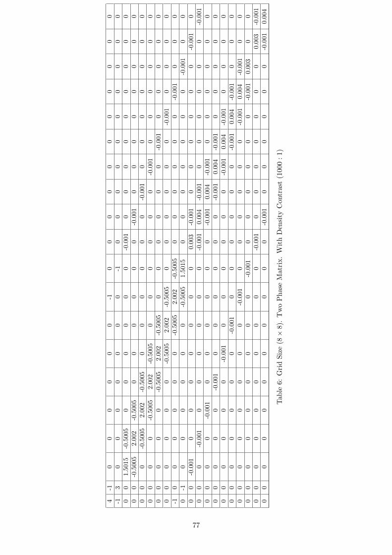
4-1

00

00

00

-10

00

00

00

00

00

-13

00

00

00

0-1

00

00

00

00

00

00

1.50

15-0

.500

50

00

00

0-0

.001

00

00

00

00

00

0-0

.500

52.

002

-0.5

005

00

00

00

-0.0

01

00

00

00

00

00

0-0

.500

52.

002

-0.5

005

00

00

00

-0.0

01

00

00

00

00

00

0-0

.500

52.

002

-0.5

005

00

00

00

-0.0

01

00

00

00

00

00

0-0

.500

52.

002

-0.5

005

00

00

00

-0.0

01

00

00

00

00

00

0-0

.500

52.0

02

-0.5

005

00

00

00

-0.0

01

00

00

-10

00

00

0-0

.5005

2.0

02

-0.5

005

00

00

00

-0.0

01

00

00

-10

00

00

0-0

.5005

1.5

015

00

00

00

0-0

.001

00

00

-0.0

010

00

00

00

0.0

03

-0.0

01

00

00

00

-0.0

01

00

00

-0.0

010

00

00

0-0

.001

0.0

04

-0.0

01

00

00

00

-0.0

01

00

00

-0.0

010

00

00

0-0

.001

0.0

04

-0.0

01

00

00

00

00

00

0-0

.001

00

00

00

-0.0

01

0.0

04

-0.0

01

00

00

00

00

00

0-0

.001

00

00

00

-0.0

01

0.0

04

-0.0

01

00

00

00

00

00

0-0

.001

00

00

00

-0.0

01

0.0

04

-0.0

01

00

00

00

00

00

0-0

.001

00

00

00

-0.0

01

0.0

04

-0.0

01

00

00

00

00

00

0-0

.001

00

00

00

-0.0

01

0.0

03

00

00

00

00

00

00

-0.0

01

00

00

00

00.0

03

-0.0

01

00

00

00

00

00

0-0

.001

00

00

00

-0.0

01

0.0

04

Tab

le6:

Gri

dS

ize

(8×

8).

Tw

oP

has

eM

atri

x.

Wit

hD

ensi

tyC

ontr

ast

(1000

:1)

77

Figure 73: 4 deflation vectors on a 8× 8 grid

C Detailed Results

C.1 Poisson Type

C.1.1 Deflated CG-with Block Incomplete Cholesky Preconditioning

Tables 74 to 76 show the results for this variant across three different grid sizes.

C.2 Two Phase

C.2.1 Deflated CG-with Block Incomplete Cholesky Preconditioning

Tables 77 to 79 show the results for this variant across three different grid sizes.

78

! ! !! ! ""#

$% !$% !$% $% !$% $%

& $' '()*(

! ! ""#

!$% !$% $% $% $% $%

& $' '()*(

!

! ""#

$% !$% $% $% $% $%

& $' '()*(

)+)),-. /)

!

+) .0#

! !

!

Figure 74: Grid Size 128× 128. Different Block Sizes and Deflation Vectors.

79

! ""#

$% $% $% $% $% $%

& $' '()*(

! !

! ! !! !! ""#

!$% !$% $% $% $% $%

& $' '()*(

! ! ""#

$% $% $% $% $+ $%

& $' '()*(

!!

!

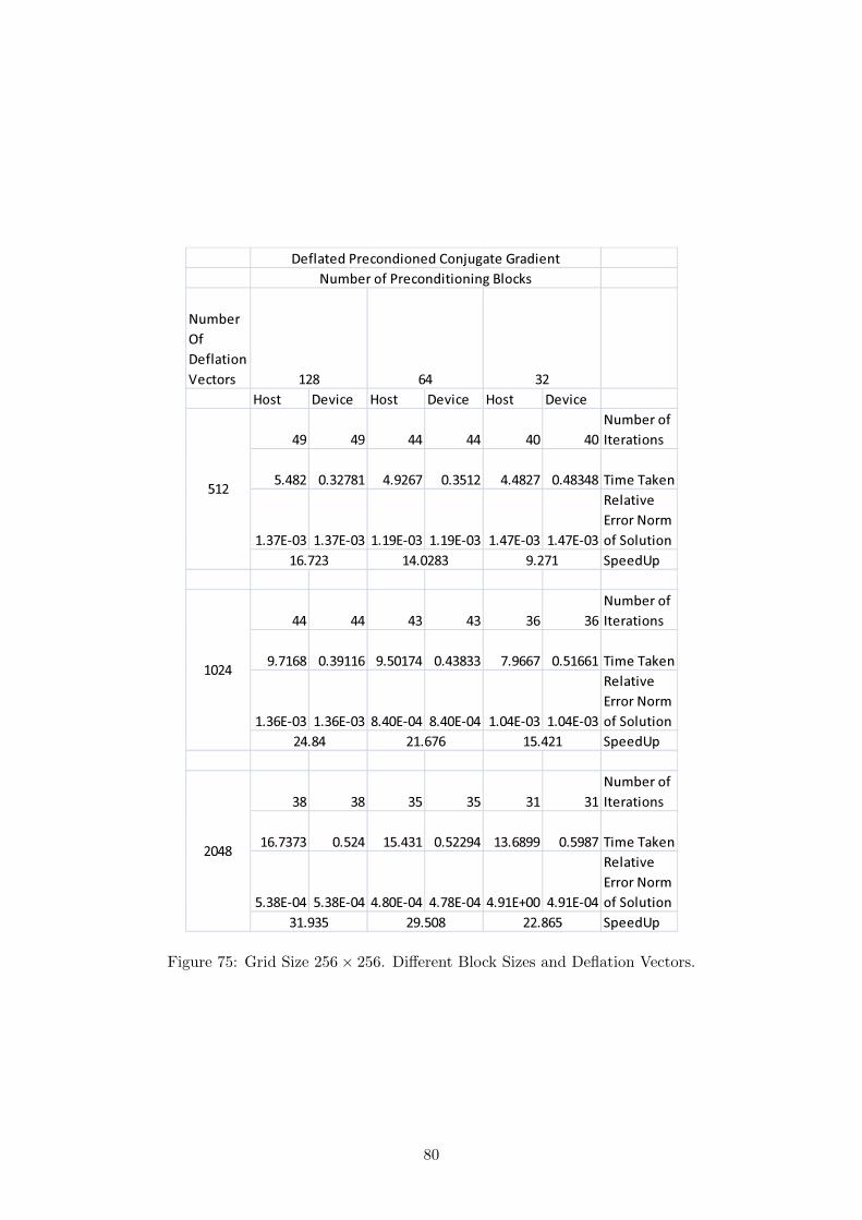
),))-./ 0) ,) /1#

!

!

Figure 75: Grid Size 256× 256. Different Block Sizes and Deflation Vectors.

80

! !! ""#

$% !$% !$% !$% $% !$%

& $' '()*(

! ! ! ! ! ""#

$% $% !$% !$% $% $%

& $' '()*(

)+)),-. /) +) .0#

!

!!

Figure 76: Grid Size 512× 512. Different Block Sizes and Deflation Vectors.

81

! ""#

$% $% $% $% $% !$%& &'()'

!! ! ! ! ""#

$% !$% $% $% $* $%& &'()'

! ""#

$* $* $% $% $% $%& &'()'

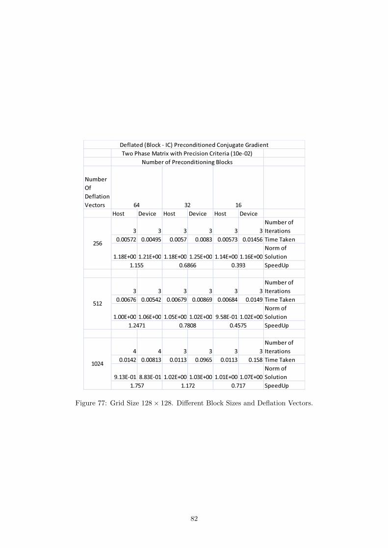
(+,#*-./( (-01 2( "3/45 63 4/- + *.

/( 1,#

!!!

! !

!

Figure 77: Grid Size 128× 128. Different Block Sizes and Deflation Vectors.

82

!

"# "# $"# "# $"# $%"#& &'()'

* *

!

"+ "+ "# $"# "# %"#& &'()'

* * * * * *

% $ $ $ !

"+$ "+ "+ $"+$ "+ %"+& &'()'

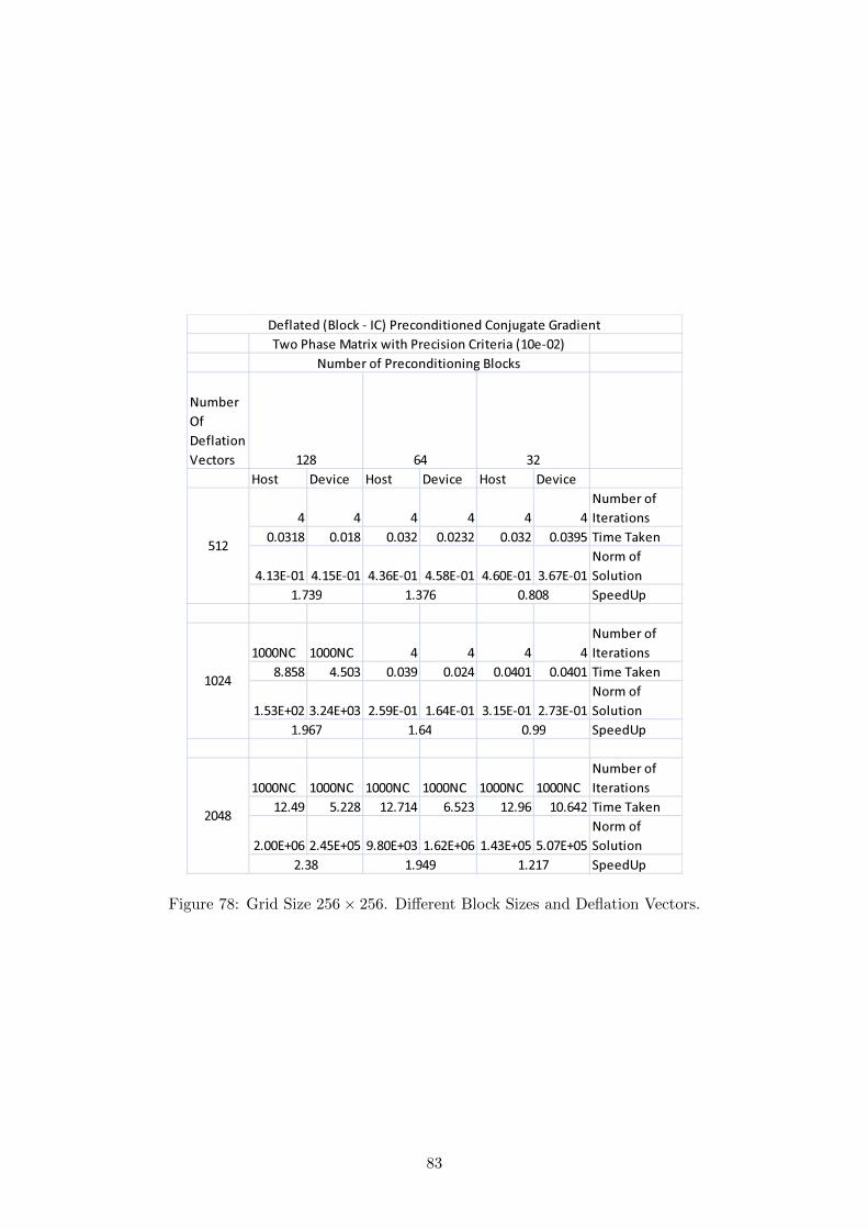
(,-!#*./( (*01 2( 3/45 63 4/* ,#.

/( 1-!

$

%$%

$% $

%

Figure 78: Grid Size 256× 256. Different Block Sizes and Deflation Vectors.

83

!"# $"# %"# !%"# "# !"#& &'()'

* * * * * *

! ! %

$"+ $"+ %"+ "+ %$"+ "+& &'()'

* * * * * *

% ! % % %$% !%

"+$ "+ %"+! %"+ !"+! "+!& &'()'

!

,( -.

! $ $

(/. #*0,( (*1- 2( 3,45 63 4,* /#0

!!

%

Figure 79: Grid Size 512× 512. Different Block Sizes and Deflation Vectors.

84